71 Worked Examples: Units, Conversion Factors & Dimensional Analysis
These worked examples have been fielded as homework problems or exam questions.
Worked Example #1
Determine the base dimensions of each of the following variables:
(a) Plane angle
(b) Specific volume
(c) Force
(d) Stress
(e) Angular velocity
(a) Plane angle: A plane angle  is defined in terms of the lines from two points meeting at a vertex and is defined by the arc length of a circle subtended by the lines and the circle’s radius. The unit of plane angle is the radian. Because it is the ratio of an arc length to the radius, the plane angle is dimensionless, i.e., a radian is one measurement unit that is already dimensionless, i.e.,
![\[ \left[ \theta \right] = 1 \]](https://eaglepubs.erau.edu/app/uploads/quicklatex/quicklatex.com-27ad2c128bcaf19cccd389dda0254d2c_l3.svg "Rendered by QuickLaTeX.com")
(b) Specific volume: The specific volume  is defined as the ratio of volume to mass, i.e., it is the reciprocal of the density. Therefore,
![\[ \left[ SV \right] = \frac{\rm L^3}{\rm M} = \rm L^3 M^{-1} = \rm M^{-1} L^3 \]](https://eaglepubs.erau.edu/app/uploads/quicklatex/quicklatex.com-26f07dee506905e8f41d8887977f445b_l3.svg "Rendered by QuickLaTeX.com")
(c) Force: Force  is the product of mass times acceleration, so
![\[ \left[ F \right] = \rm M L T^{-2} \]](https://eaglepubs.erau.edu/app/uploads/quicklatex/quicklatex.com-22e09d18abbcda6c2f96f25bcdb2d7b1_l3.svg "Rendered by QuickLaTeX.com")
(d) Stress: Stress  has dimensions of force per area, but a force is the product of mass times acceleration, so
![\[ \left[ \sigma \right] = \frac{\rm M L T^{-2}}{ \rm L^2} = \rm M L^{-1} T^{-2} \]](https://eaglepubs.erau.edu/app/uploads/quicklatex/quicklatex.com-03561fa1500823d5a4bab7ce8d11759b_l3.svg "Rendered by QuickLaTeX.com")
(e) Angular velocity: Angular velocity  is measured in terms of radians per second. A radian is unitless, so
![\[ \left[ \omega \right] = T^{-1} \]](https://eaglepubs.erau.edu/app/uploads/quicklatex/quicklatex.com-b07cc7b28c173085217f3ac2db5a6158_l3.svg "Rendered by QuickLaTeX.com")
Worked Example #2
High school students become curious about why some insects can walk on water. They discover that a fluid property of importance in this problem is called surface tension, which is given the symbol  and has dimensions of force per unit area. Write the dimensions of surface tension in terms of its base dimensions.
The units of surface tension, , are given as dimensions of force per unit area. A force is equivalent to mass times acceleration, which is MLT in base dimensions. Therefore, the base dimensions of surface tension are
![\[ \left[ \sigma_s \right] = \left( \rm M L T^{-2}\right) \rm L^{-2} = \rm M L^{-1} T^{-2} \]](https://eaglepubs.erau.edu/app/uploads/quicklatex/quicklatex.com-94b27709133b2e8cb64ee74d8994e76a_l3.svg "Rendered by QuickLaTeX.com")
Worked Example #3
Write the primary dimensions of each of the following variables from the field of thermodynamics:
(a) Energy, 
(b) Specific energy, 
(c) Power, 
(a) Energy has units of force times distance, i.e.,
![\[ \left[ E \right] = \left( \rm MLT^{-2} \right) \rm L = \rm ML^{2} T^{-2} \]](https://eaglepubs.erau.edu/app/uploads/quicklatex/quicklatex.com-c0e746fb2c60851340079c690127f735_l3.svg "Rendered by QuickLaTeX.com")
(b) Specific energy has units of energy per unit mass, i.e.,
![\[ \left[ e \right] = \rm ML^{2} T^{-2} M^{-1} = \rm L^{2} T^{-2} \]](https://eaglepubs.erau.edu/app/uploads/quicklatex/quicklatex.com-caa1dfbc382c474facb83aeb75445671_l3.svg "Rendered by QuickLaTeX.com")
(c) Power is the rate of doing work, so a force times distance per unit time, i.e.,
![\[ \left[ P \right] = \left( \rm MLT^{-2} \right) \rm L T^{-1} = \rm M L^{2} T^{-3} \]](https://eaglepubs.erau.edu/app/uploads/quicklatex/quicklatex.com-ea7af1ac425f98d04b73db1ebeed2687_l3.svg "Rendered by QuickLaTeX.com")
Worked Example #4
Determine the primary (base) dimensions of each of the following parameters from thermodynamics:
- Energy,
- Work,

- Power,
- Heat,

1. Energy, , is the ability to do work and is measured in Joules (J) in the SI system and foot-pounds (ft-lb) in the USC system. Notice that “foot-pounds” is the USC unit and not “pounds-foot” or “pounds-feet.” Energy has the same units of work (force times distance), so ![\left[ E \right] = \left( \rm MLT^{-2} \right) \rm L = \rm ML^{2} T^{-2}](https://eaglepubs.erau.edu/app/uploads/quicklatex/quicklatex.com-4fd3600ef3a34b267429023ab0238c93_l3.svg "Rendered by QuickLaTeX.com") which are the base dimensions. Notice that the units of force are obtained from the product of mass and acceleration, i.e., [] = ( M) (LT^
which are the base dimensions. Notice that the units of force are obtained from the product of mass and acceleration, i.e., [] = ( M) (LT^ = M L T.
2. Work, , is also measured in Joules (J) in the SI system and “foot-pounds” (ft-lb) in the USC system. Work is equivalent to force times distance, so ![\left[ W \right] = \rm ML T^{-2} L](https://eaglepubs.erau.edu/app/uploads/quicklatex/quicklatex.com-e1250ee76fe28b9affecc57549d13be9_l3.svg "Rendered by QuickLaTeX.com")
 M L
M L , which are the base dimensions of work.
3. Power, , is the rate of doing work and is measured in Watts (W) in the SI system and foot-pounds per second (ft-lb/s or ft-lb s in the USC system. Power is equivalent to a force times distance per unit time (or force times velocity), so
 ![\left[ P \right] = \left( \rm MLT^{-2} \right) \rm L T^{-1}](https://eaglepubs.erau.edu/app/uploads/quicklatex/quicklatex.com-0e1fb9ed20a8b5f3ca64e591e835fcaa_l3.svg "Rendered by QuickLaTeX.com")
 which are the base dimensions of power. In practice, power is measured in terms of kiloWatts (kW) in SI and horsepower (hp) in USC, where one horsepower is equivalent to 550 ft-lb/s.
4. Heat has units of energy (the ability to do work), which have the same units as work, i.e., units of Joules (J) in the SI system and foot-pounds (ft-lb) in the USC system. In base dimensions then![\left[ Q \right] = \left( \rm MLT^{-2} \right) \rm L = \rm ML^{2} \rm T^{-2}](https://eaglepubs.erau.edu/app/uploads/quicklatex/quicklatex.com-eaa8639e105ff50ed101bac072339901_l3.svg "Rendered by QuickLaTeX.com") , which are the base dimensions of heat.
, which are the base dimensions of heat.
Worked Example #5
Given that jet fuel’s average energy density is 43 to 45 Mega-Joules per kilogram), calculate the equivalent energy density in kilowatt-hours per kilogram (kWh/kg).
A Watt is a Joule per second. So, one Watt-hour is the equivalent of 3,600 Joules per hour. Therefore, one kilo-watt-hour (kWh) = 3.6 Mega-Joules (MJ). The energy density (in units of kWh/kg) = energy density (in units of MJ/kg)/3.6. Therefore, the energy density of jet fuel in kilowatt-hours per kilogram is approximately 11.9 to 12.5 kWh/kg.
Worked Example #6
Write down the Bernoulli equation and explain the meaning of each term. Verify that each of the terms in the Bernoulli equation has the exact fundamental dimensions.
The Bernoulli equation can be written as
![\[ p + \frac{1}{2} \varrho \, V^2 + \varrho g z = \mbox{constant} \]](https://eaglepubs.erau.edu/app/uploads/quicklatex/quicklatex.com-0a93eaa4d52b1b12f3dccf2856d5aab3_l3.svg "Rendered by QuickLaTeX.com")
The first term is the local static pressure, the second is the dynamic pressure, and the third is the hydrostatic pressure. The sum of the three terms is called total pressure. The Bernoulli equation is a surrogate for the energy equation in a steady, incompressible flow without losses or energy addition.
Each of the terms in the Bernoulli equation has units of pressure. In terms of fundamental dimensions, then
![\[ \left[ p \right] = ( \rm M L T^{-2} ) ( \rm L^{-2}) = \rm M L^{-1} T^{-2} \]](https://eaglepubs.erau.edu/app/uploads/quicklatex/quicklatex.com-ec27e55923f833897b6aabb57e5fcd7d_l3.svg "Rendered by QuickLaTeX.com")
![\[ \left[ \varrho \, V^2 \right] = ( \rm M L^{-3}) \rm (L^2 T^{-2}) = \rm M L^{-1} T^{-2} \]](https://eaglepubs.erau.edu/app/uploads/quicklatex/quicklatex.com-3f29714f31a5dfbf080fe773c262b5ad_l3.svg "Rendered by QuickLaTeX.com")
![\[ \left[ \varrho g z \right] = ( \rm M L^{-3}) ( \rm L T^{-2}) L = \rm M L^{-1} T^{-2} \]](https://eaglepubs.erau.edu/app/uploads/quicklatex/quicklatex.com-bdebbc626f4eecd1e99ac4c16859b937_l3.svg "Rendered by QuickLaTeX.com")
So, all terms have the same fundamental dimensions of M L T.
Worked Example #7
In each case, convert the units given into base units (can only include mass, length, and time). Show all the steps.
- N (Newton)
 mass times acceleration M L T kg m s
 - Pa (Pascal) or N m (M L T)(L) = M L T kg m s
- lb (pound) M L T slug ft s
- J (Joule) or N m (M L T) L = M L
 T kg m s
 - W (Watt) or J s (M L T) T = M L T
 kg m s
Notes: A Newton (N) is an SI unit of force but not a base unit. However, a force is equivalent to a mass times an acceleration, so in terms of base units, a Newton is equivalent to dimensions of M L T, so SI units of kg m s. A Watt (W) is the SI unit of power, which is the rate at which work is done. Work is force times distance so that power will have units of MLT L T or M L T so kg m s.
Worked Example #8
In each case, convert the numerical values in the units given into equivalent numerical values in base units (mass, length, and time). Show all the steps and state the conversion factor(s) you used.
- 3.3 l (liters) = 3.3/1,000 = 0.0033 m
 . There are 1,000 liters in a cubic meter.
 - 1.2 hrs (hours) = 3,600
 1.2 = 4,320 s. There are 3,600 seconds in an hour.
 - 15.6 hp (horsepower) = 15.6 550 = 8,580 ft-lb s. Notice: 550 ft-lb s is equivalent to one horsepower.
- 12.8 gals (US gallons) = 12.8 0.13368 = 1.711 ft. One gallon equals 0.13368 ft.
- 12.4 kN cm = 12.4
 Pa = 12.4
  kg m s. One kN = 1,000 N, and there are 1,000 square centimeters in a square meter.
Notes: Converting units takes some work, but it is essential to do it correctly. The first step is to realize and accept that many quantities measured daily are not base quantities but need to be converted to base quantities for engineering calculations. Volume is often measured in liters, but it is not a base unit. There are 1,000 liters in a cubic meter; a meter is a base SI unit. James Watt figured out from experiments with Scottish farm horses that one horsepower (hp) was equivalent to a rate of doing work of 550 foot-pounds per second or 550 ft-lb s, so 550 is the conversion factor from hp to base USC units.
Worked Example #9
In a particular fluids problem, the flow rate, , depends on a height,  , and acceleration under gravity,
  . The relationship can be expressed as
![\[ Q = K \, h^{\alpha} \, g^{\beta} \]](https://eaglepubs.erau.edu/app/uploads/quicklatex/quicklatex.com-adc6827b44c5a2f7fe618400a7a63bf6_l3.svg "Rendered by QuickLaTeX.com")
where  is a constant with dimensions of length. By satisfying dimensional homogeneity, determine the values of
  and
and  .
.
In terms of the dimensions
![\[ \left[ Q\right] = L \left[ h^{\alpha} \right] \left[ g^{\beta} \right] \]](https://eaglepubs.erau.edu/app/uploads/quicklatex/quicklatex.com-ccec742165e812827edc613a06810e66_l3.svg "Rendered by QuickLaTeX.com")
and so for each parameter, then
![\[ \left[ Q \right] = \rm L^3 T^{-1} \quad\quad \left[ K \right] = \rm L \quad\quad \left[ h \right] = \rm L \quad\quad \left[ g \right] = \rm L T^{-2} \]](https://eaglepubs.erau.edu/app/uploads/quicklatex/quicklatex.com-545d1f2dad776f98c224327221eb15f6_l3.svg "Rendered by QuickLaTeX.com")
Therefore,
![\[ \rm L^3 T^{-1} = \rm L^{1} \, \left( \rm L \right)^\alpha \, \left( \rm L T^{-2}\right)^\beta \]](https://eaglepubs.erau.edu/app/uploads/quicklatex/quicklatex.com-15a2c05478d221b56d1c586dd9cad7a0_l3.svg "Rendered by QuickLaTeX.com")
To obtain dimensional homogeneity, then

so  and
and  . Inserting the values gives the relationship as
![\[ Q = K \, h^{3/2} \, g^{1/2} = K \, \sqrt{g} \, h^{3/2} \]](https://eaglepubs.erau.edu/app/uploads/quicklatex/quicklatex.com-f817a2e9c18d88c7d09c044c163bf254_l3.svg "Rendered by QuickLaTeX.com")
Worked Example #10
A small jet airplane has a mean chord of 1.5 m and flies at a Mach number of 0.7 in conditions equivalent to those in the ISA. If the Reynolds number, based on mean chord length, is  , at what approximate pressure altitude,
  , is it flying? Assume that
  and
and  depend on absolute temperature, i.e.,
  and
and  . Also, assume a reference pressure altitude of
  = 10,000 m where
  = 299.53 m/s,
  = 3.5251
  m/s, and
  = 223.25 K. Finally, assume for the ISA that
  where
where  = 6.5 K per 1,000 m.
This problem gives minimal information besides the Mach number, Reynolds number, and wing chord. The Mach number at altitude (alt) is
![\[ M_{\rm alt} = \dfrac{V_{\rm alt}}{a_{\rm alt}} = 0.7 \]](https://eaglepubs.erau.edu/app/uploads/quicklatex/quicklatex.com-7ecbfa3990aae82171fcdbd8d5e6825d_l3.svg "Rendered by QuickLaTeX.com")
and the corresponding Reynolds number is
![\[ Re_{\rm alt} = \dfrac{\varrho_{\rm alt} \, V_{\rm alt} \, c}{\mu_{\rm alt}} = \dfrac{V_{\rm alt} \, c}{\nu_{\rm alt}} = 8.75 \times 10^6 \]](https://eaglepubs.erau.edu/app/uploads/quicklatex/quicklatex.com-d51faf370994de83ab858bec06bb2d9c_l3.svg "Rendered by QuickLaTeX.com")
where is the kinematic viscosity and  is the wing chord. Notice that the airspeed
  appears in both parameters, which can be written as
![\[ V_{\rm alt} = a_{\rm alt} \, M_{\rm alt} \]](https://eaglepubs.erau.edu/app/uploads/quicklatex/quicklatex.com-4bf13bfea7f78e43bfc737124c30acc5_l3.svg "Rendered by QuickLaTeX.com")
and
![\[ Re_{\rm alt} = \dfrac{a_{\rm alt} \, M_{\rm alt} \, c}{\nu_{\rm alt}} \]](https://eaglepubs.erau.edu/app/uploads/quicklatex/quicklatex.com-9f4aa6bccc9724ea5d36a81c8adadd3a_l3.svg "Rendered by QuickLaTeX.com")
so the ratio  is given by
![\[ \dfrac{a_{\rm alt}}{\nu_{\rm alt}} =\dfrac{Re_{\rm alt}}{M_{\rm alt} \, c} = \dfrac{8.75 \times 10^6}{0.7 \times 1.5} = 8.33 \times 10^6 \]](https://eaglepubs.erau.edu/app/uploads/quicklatex/quicklatex.com-f666ee769d075adcd339f3045a49c821_l3.svg "Rendered by QuickLaTeX.com")
Also, both and depend on absolute temperature, i.e.,
![\[ a_{\rm alt} \quad \propto \quad \sqrt{T_{\rm alt}} \]](https://eaglepubs.erau.edu/app/uploads/quicklatex/quicklatex.com-5e15640994b7580642d750fb5c6228c3_l3.svg "Rendered by QuickLaTeX.com")
and
![\[ \nu_{\rm alt} \quad \propto \quad T_{\rm alt}^{3/2} \]](https://eaglepubs.erau.edu/app/uploads/quicklatex/quicklatex.com-87eb15fccafb0193684335917b0438e9_l3.svg "Rendered by QuickLaTeX.com")
therefore the ratio is
![\[ \dfrac{a_{\rm alt}}{\nu_{\rm alt}} \quad \propto \quad \dfrac{1}{T_{\rm alt}} \]](https://eaglepubs.erau.edu/app/uploads/quicklatex/quicklatex.com-5632484c39fa9425ee19af8db736be9e_l3.svg "Rendered by QuickLaTeX.com")
Therefore,
![\[ \dfrac{ \left( \dfrac{a}{\nu} \right)_{\rm alt}}{ \left( \dfrac{a}{\nu} \right)_{\rm ref}} = \dfrac{T_{\rm ref}}{T_{\rm alt}} \]](https://eaglepubs.erau.edu/app/uploads/quicklatex/quicklatex.com-31eaa808f15ed1e823a713339a63d845_l3.svg "Rendered by QuickLaTeX.com")
The ratio  and can be taken at some assumed (a guess) reference altitude in the ISA. Assume a height of 10,000 m, which is probably close to where the aircraft is flying if it is a small jet cruising at Mach 0.7. Using the ISA properties at 10,000 m then, = 299.53 m/s, = 3.5251 m/s, and = 223.25 K. Solving for
  gives
gives
![\[ T_{\rm alt} = T_{\rm ref} \left( \dfrac{ \left( \dfrac{a}{\nu} \right)_{\rm ref}}{ \left( \dfrac{a}{\nu} \right)_{\rm alt}} \right) = 223.25 \left( \dfrac{ 8.5 \times 10^6}{8.33 \times 10^6} \right) = 227.81~\mbox{K} \]](https://eaglepubs.erau.edu/app/uploads/quicklatex/quicklatex.com-8739580e3a9bd26f2eea6f3d6b0976d6_l3.svg "Rendered by QuickLaTeX.com")
Therefore, the pressure altitude corresponding to this standard temperature in the ISA is
![\[ h_{\rm alt} = \dfrac{T_0 - T_{\rm alt}}{B} = \dfrac{288.15 - 227.81}{0.0065} = 9,283~\mbox{m} \]](https://eaglepubs.erau.edu/app/uploads/quicklatex/quicklatex.com-6a9fbe5b01a02b0979b5c764c43ef840_l3.svg "Rendered by QuickLaTeX.com")
which, by rechecking the Reynolds number and Mach number, is a reasonably good estimate of the pressure altitude at which the airplane is flying.
Worked Example #11
A student wants to know the drag on a full-scale race car with a length  and travels at a speed
  . The student constructs a
  -scale model of the race car and measures the drag on the model in a wind tunnel under dynamically similar conditions. The student claims that the drag force on the full-scale race car will be identical to that of the -scale model. Is this claim correct? Explain. Ignore compressibility effects.
In the wind tunnel, we want to match the Reynolds numbers between the actual car and the model to achieve flow similarity. The Reynolds number for the actual vehicle can be written as
![\[ Re_1 = \frac{\varrho V_1 L_1}{\mu} \]](https://eaglepubs.erau.edu/app/uploads/quicklatex/quicklatex.com-7bb9d4eb2abc23fa07999e1f8aa5e00d_l3.svg "Rendered by QuickLaTeX.com")
and for the model
![\[ Re_2 = \frac{\varrho V_2 L_2}{\mu} \]](https://eaglepubs.erau.edu/app/uploads/quicklatex/quicklatex.com-80ce9b06e68991949d2039deb07df64c_l3.svg "Rendered by QuickLaTeX.com")
Therefore, we have that
![\[ \frac{Re_2}{Re_1} = 1 = \frac{V_2 L_2}{V_1 L_1} \]](https://eaglepubs.erau.edu/app/uploads/quicklatex/quicklatex.com-055185c0301497cb8a20f6fc4abaaa6f_l3.svg "Rendered by QuickLaTeX.com")
if the flow conditions (e.g., temperature and pressure, hence its density and viscosity) are the same in the wind tunnel as those for the actual car. The ratio  , so
, so
![\[ V_2 = f \, V_1 \]](https://eaglepubs.erau.edu/app/uploads/quicklatex/quicklatex.com-8ba616d8783096d695a33ed234f54a91_l3.svg "Rendered by QuickLaTeX.com")
The drag force on the actual car can be written as
![\[ D_1 = \frac{1}{2} \varrho V_1^2 A_1 C_D \]](https://eaglepubs.erau.edu/app/uploads/quicklatex/quicklatex.com-8412d831208e39ef06529de9087a1344_l3.svg "Rendered by QuickLaTeX.com")
where  is a reference area on which the drag coefficient
  is based. It is reasonable to assume the drag coefficient of both the actual car and the model is the same, which is typical of bluff bodies like cars. The drag force on the model can be written as
![\[ D_2 = \frac{1}{2} \varrho V_2^2 A_2 C_D \]](https://eaglepubs.erau.edu/app/uploads/quicklatex/quicklatex.com-d9244d543dd5728eda8d0434e8a438ae_l3.svg "Rendered by QuickLaTeX.com")
where the ratio  , i.e., lengths scale linearly but areas scale by the square. Therefore, we can write
![\[ \frac{D_2}{D_1} = \left( \frac{V_2}{V_1} \right)^2 \ \frac{A_2}{A_1} = \left( \frac{f V_1}{V_1} \right)^2 \ \frac{1}{f^2} = 1 \]](https://eaglepubs.erau.edu/app/uploads/quicklatex/quicklatex.com-8eff000de7fb14147ae1aceac77bd0c4_l3.svg "Rendered by QuickLaTeX.com")
So, the student is correct! This is an interesting and useful outcome that follows from the scaling relationships. The force on a body of a particular shape at a given Reynolds number is the same regardless of the combination of size and speed used to produce that given Reynolds number. Of course, the flow conditions (e.g., temperature and pressure, hence density and viscosity) must also be the same.
Worked Example #12
Consider the drag of a sphere problem using the Buckingham  method, previously performed using the repeating variables
  ,
,  , and
, and  . Repeat the dimensional analysis process using ,
  , and as the repeating variables. Show all of your work. Comment on the results you obtained.
The relationship between  and the air properties may be written in a general functional form as
![\[ D = \phi \left( \varrho_{\infty}, \, V_{\infty}, \, \mu_{\infty}, \, d \right) \]](https://eaglepubs.erau.edu/app/uploads/quicklatex/quicklatex.com-8c269d5ab9d4d3629e55016ce84d9f39_l3.svg "Rendered by QuickLaTeX.com")
where is the dependent variable. , , , and are the independent variables. In implicit form, the drag can be written as
![\[ \psi \left( \varrho_{\infty}, \, V_{\infty}, \, \mu_{\infty}, \, d, \, D \right) = 0 \]](https://eaglepubs.erau.edu/app/uploads/quicklatex/quicklatex.com-e673b84f3cb01d4056ddb9e6dd764d0f_l3.svg "Rendered by QuickLaTeX.com")
For each dependency, then
![\begin{eqnarray*} \left[ D \right] & = & \rm M L T^{-2} \\ \left[ \varrho_{\infty} \right] & = & \rm ML^{-3} \\ \left[ V_{\infty} \right] & = & \rm LT^{-1} \\ \left[ \mu_{\infty} \right] & = & \rm ML^{-1} \rm T^{-1} \\ \left[ d \right] & = & \rm L \end{eqnarray*}](https://eaglepubs.erau.edu/app/uploads/quicklatex/quicklatex.com-f9aaee5b61c62a3384e1071129a318c4_l3.svg "Rendered by QuickLaTeX.com")
Setting up the dimensional matrix gives
![\[ \begin{array}{l|r|r|r|r|r|r} \mbox{\small Base~unit} & D & \varrho_{\infty} & V_{\infty} & d & \mu_{\infty} \\ \hline \mbox{\small Mass M:} & 1 & 1 & 0 & 0 & 1 \\ \mbox{\small Length L:} & 1 & -3 & 1 & 1 & -1 \\ \mbox{\small Time T:} & -2 & 0 & -1 & 0 & -1 \end{array} \]](https://eaglepubs.erau.edu/app/uploads/quicklatex/quicklatex.com-6f3d735436774181e41ff541722367b3_l3.svg "Rendered by QuickLaTeX.com")
Choose  and as repeating variables. These can be confirmed by finding the determinant of the dimensional submatrix that is formed by the repeating variables, which shows that
![\[ \det \begin{bmatrix} 1 & 0 & 0 \\ -1 & 1 & -1 \\ -1 & -1 & 0 \end{bmatrix} \ne 0 \]](https://eaglepubs.erau.edu/app/uploads/quicklatex/quicklatex.com-78a95aca39365cfe3f9a696d98e7cfb8_l3.svg "Rendered by QuickLaTeX.com")
Following the Buckingham method, then the products for this problem are determined from
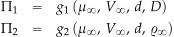
For the first product
![\[ \Pi_{1} = (\mu_{\infty})^{\alpha} \, (V_{\infty})^{\beta} \, (d)^{\gamma} \, D \]](https://eaglepubs.erau.edu/app/uploads/quicklatex/quicklatex.com-9c2691f812d1a2a8af6f670ef957b486_l3.svg "Rendered by QuickLaTeX.com")
The values of the coefficients , , and  must be obtained to make the equation dimensionally homogeneous. In terms of the dimensions of the parameters, then
![\[ \left[ \Pi_{1} \right] = 1 = \rm M^{0}L^{0}T^{0} = \left( \rm ML^{-1}T^{-1} \right)^{\alpha} \left( \rm LT^{-1} \right)^{\beta} \left( \rm L \right)^{\gamma} \left( \rm MLT^{-2} \right) \]](https://eaglepubs.erau.edu/app/uploads/quicklatex/quicklatex.com-daea479a1202bb450b4d48abff4fc45b_l3.svg "Rendered by QuickLaTeX.com")
For  to be dimensionless, then the powers or exponents of M, L, and T must add to zero, i.e.,
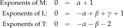
By inspection  ,
,  , and
, and  . So, the first product is
![\[ \Pi_{1} = (\mu_{\infty})^{\alpha}\, (V_{\infty})^{\beta} \, (d)^{\gamma} \, D = \mu_{\infty}^{-1} \, V_{\infty}^{-1} \, d^{-1} \, D \]](https://eaglepubs.erau.edu/app/uploads/quicklatex/quicklatex.com-fab21e118d37b2cb84ac93fe66db4c5a_l3.svg "Rendered by QuickLaTeX.com")
or
![\[ \Pi_{1} = \frac{D}{\mu_{\infty} \, V_{\infty} \, d} \]](https://eaglepubs.erau.edu/app/uploads/quicklatex/quicklatex.com-e3a68eab7df6e2cdc03ca489b2ab4f09_l3.svg "Rendered by QuickLaTeX.com")
which is still dimensionless, but it is a different grouping from what was obtained with  , and as the repeating variables.
This is an interesting outcome because this parameter is a form of Stokes’ Law, which Sir George Stokes determined in the 1840s. He found that the drag force on a sphere of radius  moving through a fluid of viscosity
  at a very low speed is given by
![\[ D = 6 \pi R \mu V \]](https://eaglepubs.erau.edu/app/uploads/quicklatex/quicklatex.com-08de2bdaf46c77d7718d2be6324603cf_l3.svg "Rendered by QuickLaTeX.com")
Comments: This drag force is proportional to the sphere’s radius. This outcome is not obvious because, based on what was done before, it might be thought that drag would be proportional to the cross-sectional area, which would vary as the square of the radius. The drag force is also directly proportional to the speed and  . But this behavior ONLY occurs at very low Reynolds numbers near unity. This outcome was obtained by emphasizing viscosity over density
  in the repeating variables. When choosing the repeating variables, a general rule is that they must have an important effect on the dependent variable, in this case, the drag. So, by emphasizing viscosity, in this case, a different dimensionless grouping has been obtained.
Therefore, in this case, then
![\[ {\Pi_{1} = C_{D_{\rm Stokes}} = \frac{D}{3 \pi \, \mu_{\infty} \, V_{\infty} \, d} } \]](https://eaglepubs.erau.edu/app/uploads/quicklatex/quicklatex.com-02693356ceb5cd26f0f6cc1afea0bb8d_l3.svg "Rendered by QuickLaTeX.com")
For the second product then
![\[ \Pi_{2} = (\mu_{\infty})^{\alpha} \, (V_{\infty})^{\beta} \, (d)^{\gamma} \, \varrho_{\infty} \]](https://eaglepubs.erau.edu/app/uploads/quicklatex/quicklatex.com-2bec33ed140e516bc15bec8b5ce90cde_l3.svg "Rendered by QuickLaTeX.com")
so
![\[ \left[ \Pi_{2} \right] = 1 = \rm M^{0} \rm L^{0} \rm T^{0} = \left(\rm M L^{-1} T^{-1} \right)^{\alpha} \left( \rm LT^{-1} \right)^{\beta} \left(\rm L \right)^\gamma \left( ML^{-3} \right) \]](https://eaglepubs.erau.edu/app/uploads/quicklatex/quicklatex.com-26b06de688736a865433d19acf67914f_l3.svg "Rendered by QuickLaTeX.com")
and setting the sum of the powers to zero gives
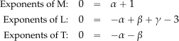
The solution is ,  , and
, and  and so
![\[ \Pi_{2} = (\mu_{\infty})^{\alpha} \, (V_{\infty})^{\beta} \, (d)^{\gamma} \, \varrho_{\infty} = \mu_{\infty}^{-1} \, V_{\infty}^{1} \, d^{1} \, \varrho_{\infty} \]](https://eaglepubs.erau.edu/app/uploads/quicklatex/quicklatex.com-8da5561a5e9854c6da790eaaf7859e9c_l3.svg "Rendered by QuickLaTeX.com")
i.e.,
![\[ \Pi_{2} = \frac{\varrho_{\infty} \, V_{\infty} \, d}{\mu_{\infty}} \]](https://eaglepubs.erau.edu/app/uploads/quicklatex/quicklatex.com-d20a98edbf91ce9fbdc24c90f9d0536a_l3.svg "Rendered by QuickLaTeX.com")
which will be recognized as the Reynolds number.
Therefore, as a result of the dimensional analysis of the sphere, then
![\[ \phi_1 \left( \frac {D}{3 \pi\mu \, V_{\infty} d}, \frac{\varrho_{\infty} \, V_{\infty} \, d}{\mu_{\infty}} \right) = 0 \]](https://eaglepubs.erau.edu/app/uploads/quicklatex/quicklatex.com-b53d9a51860bd3fbf8e90952b994f93e_l3.svg "Rendered by QuickLaTeX.com")
or
![\[ \phi_1 \left( C_{D_{\rm Stokes}}, Re \right) = 0 \]](https://eaglepubs.erau.edu/app/uploads/quicklatex/quicklatex.com-59f68a84d4f172f669a02b0ab50a9c7c_l3.svg "Rendered by QuickLaTeX.com")
or in explicit form
![\[ C_{D_{\rm Stokes}} = \phi_2 \left( Re \right) \]](https://eaglepubs.erau.edu/app/uploads/quicklatex/quicklatex.com-1579b5dc4f61c97d072dcc129a208d61_l3.svg "Rendered by QuickLaTeX.com")
Worked Example #13
Based on experiments performed in a low-speed wind tunnel, it is determined that the power required at the shaft to drive a propeller forward is a function of the thrust the propeller produces, , the size of the propeller as characterized by its diameter , the rotational speed of the propeller in terms of revolutions per second  , and the air density , and the operating freestream velocity . Find the appropriate dimensionless groupings that will describe this problem.
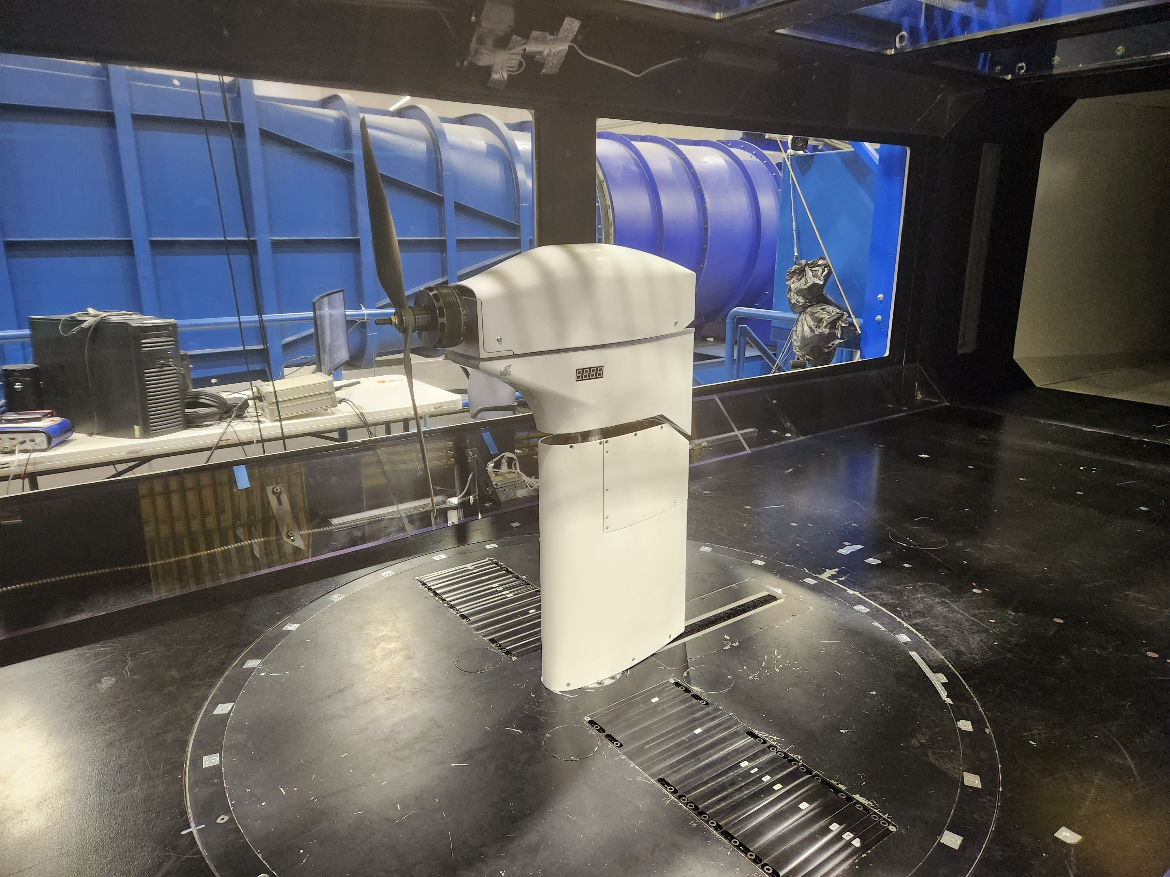
The power required for the propeller (the dependent variable), , can be written in a functional form as
![\[ P = \phi_1(F, \, d, \varrho_{\infty}, \, n, \, V_{\infty}) \]](https://eaglepubs.erau.edu/app/uploads/quicklatex/quicklatex.com-cef7dca0e91df9fbbeb8fe37ef0a4a07_l3.svg "Rendered by QuickLaTeX.com")
where  is the function to be determined. The power would be given by
  , where is the torque and
  is the angular velocity in radians per second.
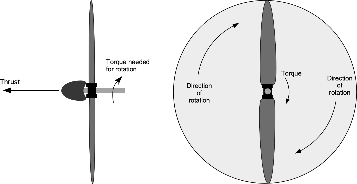 The preceding equation can be written in an implicit form as
![\[ \phi_2(F, \, d, \, \varrho_{\infty}, \, n, \, V_{\infty}, \, P) = 0 \]](https://eaglepubs.erau.edu/app/uploads/quicklatex/quicklatex.com-99f8b57ca182a370770d6415b764a71e_l3.svg "Rendered by QuickLaTeX.com")
In this case, there are six variables ( ) and three fundamental dimensions (
 ) comprising mass (
 ), length (), and time (
 ). This means that
  , so three products must be determined.
The functional dependence can also be written in the form
![\[ \phi_3 (\Pi_1, \, \Pi_2, \, \Pi_3) = 0 \]](https://eaglepubs.erau.edu/app/uploads/quicklatex/quicklatex.com-97b9f05d8606277b06bd495b44ca3faf_l3.svg "Rendered by QuickLaTeX.com")
where  ,
,  and are the dimensionless groupings to be determined.
Choose the variables , , and as the repeating variables, which are all linearly independent and can be confirmed using the dimensional matrix (below). The dimensionless products can each be written in terms of these repeating variables plus one other variable, that is
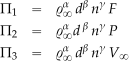
where in each case, the powers , , and are to be determined so that each of the products must be dimensionless.
Now, the base dimensions of each variable can be written down. For this problem, then
![\begin{eqnarray*} \left[ \varrho_{\infty} \right] & = & \rm M L^{-3} \\ \left[ d \right] & = & \rm L \\ \left[ V_{\infty} \right] & = & \rm L T^{-1} \\ \left[ n \right] & = &\rm T^{-1} \\ \left[ F \right] & = & \rm M L T^{-2} \\ \left[ P \right] & = & (\rm M L T^{-2}) (\rm L T^{-1}) = \rm M L^2 T^{-3} \end{eqnarray*}](https://eaglepubs.erau.edu/app/uploads/quicklatex/quicklatex.com-9f400eb214f98f772f0f22c80e94add0_l3.svg "Rendered by QuickLaTeX.com")
and so the dimensional matrix is
![\[ \begin{array}{l|r|r|r|r|r|r} \mbox{\small Base~unit} & \varrho_{\infty} & d & V_{\infty} & n & F & P \\ \hline \text{\small Mass M:} & 1 & 0 & 0 & 0 & 1 & 1 \\ \text{\small Length L:} & -3 & 1 & 1 & 0 & 1 & 2 \\ \text{\small Time T:} & 0 & 0 & -1 & -1 & -2 & -3 \end{array} \]](https://eaglepubs.erau.edu/app/uploads/quicklatex/quicklatex.com-e872ef15027fe1bfdd99735e2fd5feb1_l3.svg "Rendered by QuickLaTeX.com")
Finding the determinant of the dimensional submatrix that is formed by the repeating variables shows that
![\[ \det \begin{bmatrix} 1 & 0 & 0 \\ -3 & 1 & 0 \\ 0 & 0 & 1 \end{bmatrix} \ne 0 \]](https://eaglepubs.erau.edu/app/uploads/quicklatex/quicklatex.com-4c9a35992fdb0d2e1d17558456ec1be6_l3.svg "Rendered by QuickLaTeX.com")
So the selected repeating variables are linearly independent.
Considering the first product then
![\[ \Pi_ 1 = \varrho_{\infty}^\alpha \, d^\beta \, n^\gamma \, F \]](https://eaglepubs.erau.edu/app/uploads/quicklatex/quicklatex.com-39edb1be9336e627ffa071203f4be540_l3.svg "Rendered by QuickLaTeX.com")
where , , and are to be determined. The dimensions of the product are dimensionless, i.e.,
![\[ \left[ \Pi_1 \right] = \rm M^0 L^0 T^0 = 1 \]](https://eaglepubs.erau.edu/app/uploads/quicklatex/quicklatex.com-511af9d75c6df04fb43bd481d7a14772_l3.svg "Rendered by QuickLaTeX.com")
In terms of the base dimensions of the parameters, then
![\[ (\rm M L^{-3})^\alpha \, (\rm L)^\beta \, (\rm T^{-1})^\gamma \, \rm (M L T^{-2}) = \rm M^0 L^0 T^0 \]](https://eaglepubs.erau.edu/app/uploads/quicklatex/quicklatex.com-beca4a8ce082b3b382d26219b8a828ca_l3.svg "Rendered by QuickLaTeX.com")
Making the equation dimensionally homogeneous by equating the exponents for each of the dimensions, in turn, gives
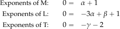
These simultaneous equations have the solution that ,  and
and  . Therefore, the first product can be written as
![\[ \Pi_1 = \varrho_{\infty}^{-1} \, d^{-4} \, n^{-2} \, F = \frac{F}{\varrho_{\infty} \, n^2 \, d^4} = C_T \]](https://eaglepubs.erau.edu/app/uploads/quicklatex/quicklatex.com-ae35609bd4a87587c52c49e17c926b76_l3.svg "Rendered by QuickLaTeX.com")
Which is a form of thrust coefficient, i.e., a dimensionless measure of thrust.
Considering now the second product then
![\[ \Pi_2 = \varrho_{\infty}^\alpha \, d^\beta \, n^\gamma \, P \]](https://eaglepubs.erau.edu/app/uploads/quicklatex/quicklatex.com-42978f9dc9ca882b6387a7c30c23a605_l3.svg "Rendered by QuickLaTeX.com")
where new values for , , and are to be determined. In terms of dimensions
![\[ \left[ \Pi_2 \right] = (\rm M L^{-3})^\alpha \, (\rm L)^\beta \, (\rm T^{-1})^\gamma \, (\rm M L^2 T^{-3} ) = \rm M^0 L^0 T^0 = 1 \]](https://eaglepubs.erau.edu/app/uploads/quicklatex/quicklatex.com-b4fcf4cbf244fedd0c6ed1de23379eba_l3.svg "Rendered by QuickLaTeX.com")
Making this latter equation dimensionally homogeneous gives
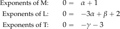
These equations have the solution that  ,
,  and
and  . Therefore, the second product is
![\[ \Pi_2 = \varrho_{\infty}^{-1} \, d^{-5} \, n^{-3} \, F = \frac{P}{\varrho_{\infty} \, n^3 \, d^5} = C_P \]](https://eaglepubs.erau.edu/app/uploads/quicklatex/quicklatex.com-d6ddb089fbd795a2e9226bfa067d3196_l3.svg "Rendered by QuickLaTeX.com")
which is a form of power coefficient, i.e., a dimensionless measure of power.
Finally, for the third product, then
![\[ \Pi_3 = \varrho_{\infty}^\alpha \, d^\beta \, n^\gamma \, V_{\infty} \]](https://eaglepubs.erau.edu/app/uploads/quicklatex/quicklatex.com-60ad8e0b472d3621821ba5c2bdd98973_l3.svg "Rendered by QuickLaTeX.com")
and in terms of dimensions, then
![\[ \left[ \Pi_3 \right] = (\rm M L^{-3})^\alpha (L)^\beta (\rm T^{-1})^\gamma (\rm L T^{-1} ) = \rm M^0 L^0 T^0 = 1 \]](https://eaglepubs.erau.edu/app/uploads/quicklatex/quicklatex.com-864a0a3f96b948cc837b965562032118_l3.svg "Rendered by QuickLaTeX.com")
Making this final equation dimensionally homogeneous gives
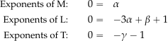
These latter equations have the solution that  , and . Therefore, the third product is
![\[ \Pi_3 = \varrho_{\infty}^{0} \, d^{-1} \, n^{-1} \, \, V_{\infty} = \frac{V_{\infty}}{n \, d} = J \]](https://eaglepubs.erau.edu/app/uploads/quicklatex/quicklatex.com-20f0635da8548fccffe699ed4bd1ce1c_l3.svg "Rendered by QuickLaTeX.com")
which is a dimensionless airspeed called a tip speed ratio or advance ratio.
Therefore, for this propeller problem, then
![\[ \phi \left( \frac{F}{\varrho_{\infty} \, n^2 \, d^4}, \frac{P}{\varrho_{\infty} \, n^3\, d^5} , \frac{V_{\infty}}{n \, d} \right) = 0 \]](https://eaglepubs.erau.edu/app/uploads/quicklatex/quicklatex.com-3d49edaf44be1523570d6309e03224a8_l3.svg "Rendered by QuickLaTeX.com")
or
![\[ \frac{P}{\varrho_{\infty} n^3 \, d^5} = \phi_0 \left( \frac{F}{\varrho_{\infty} \, n^2 \, d^4}, \frac{V_{\infty}}{n \, d} \right) = 0 \]](https://eaglepubs.erau.edu/app/uploads/quicklatex/quicklatex.com-57475f7882c704777f743831a3e5b906_l3.svg "Rendered by QuickLaTeX.com")
or finally as
![\[ C_P = \phi_0 \left( C_T, \, J \right) \]](https://eaglepubs.erau.edu/app/uploads/quicklatex/quicklatex.com-2bec32383a53eedf18deaa63777eaec1_l3.svg "Rendered by QuickLaTeX.com")
This outcome allows us to evaluate the propeller’s performance in terms of power coefficient as a function of the thrust coefficient and the tip speed ratio.
Worked Example #14
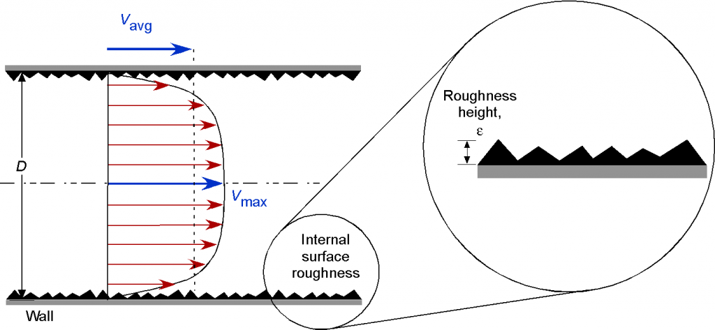
Consider the internal turbulent flow through a rough pipe. The objective is to determine the dimensionless groupings that will describe this problem. The dependencies include the average flow velocity  , the diameter of the pipe, , the density of the fluid flowing through the pipe , the viscosity of the fluid, , the roughness height of the pipe
  , and the pressure drop along the length of the pipe,
  .
.
Proceeding using the Buckingham method, then in the general functional form
![\[ \phi (V_{\rm av}, \, d, \, \varrho, \, \mu, \, \epsilon, \, dp/dx ) = 0 \]](https://eaglepubs.erau.edu/app/uploads/quicklatex/quicklatex.com-b37a956f3c363a9323e5d381f05b3ad7_l3.svg "Rendered by QuickLaTeX.com")
In this case, there are six variables () and three fundamental dimensions () comprising mass (), length (), and time (). According to the Buckingham Method, then , so there are three products.
The dimensional matrix is
![\[ \begin{array}{l|r|r|r|r|r|c} \mbox{\small Base~unit} & V_{\rm av} & d & \varrho &\mu & \epsilon & dp/dx \\ \hline \text{\small Mass M:} & 0 & 0 & 1 & 1 & 0 & 1 \\ \text{\small Length L:} & 1 & 1 & -3 & -1 & 1 & -2 \\ \text{\small Time T:} & -1 & 0 & 0 & -1 & 0 & -2 \end{array} \]](https://eaglepubs.erau.edu/app/uploads/quicklatex/quicklatex.com-40f1fb60d2be60816429ff4cde770642_l3.svg "Rendered by QuickLaTeX.com")
Choose , , and as the repeating variables, a common choice for fluid problems, which contain all of the base dimensions. Finding the determinant of the dimensional submatrix that is formed by the repeating variables shows that
![\[ \det \begin{bmatrix} 1 & 0 & 0 \\ -3 & 1 & 1 \\ 0 & 0 & 0 \end{bmatrix} \ne 0 \]](https://eaglepubs.erau.edu/app/uploads/quicklatex/quicklatex.com-46cf767d05aa13d5af6a953bed06606a_l3.svg "Rendered by QuickLaTeX.com")
so the selected repeating variables are linearly independent.
Considering the first product then
![\[ \Pi_1 = \varrho^\alpha \, V_{\rm av}^\beta \, d^\gamma \, \mu \]](https://eaglepubs.erau.edu/app/uploads/quicklatex/quicklatex.com-d526b89e49c0bf57609853590685e8dc_l3.svg "Rendered by QuickLaTeX.com")
and in terms of dimensions, then
![\[ \left[ \Pi_1 \right] = (\rm ML^{-3})^\alpha (\rm LT^{-1})^\beta (\rm L)^\beta \rm \rm M L^{-1} T^{-1} = M^0 L^0 T^0 = 1 \]](https://eaglepubs.erau.edu/app/uploads/quicklatex/quicklatex.com-80bcfa64ec1122812eba7e68d38a6298_l3.svg "Rendered by QuickLaTeX.com")
Making the equation dimensionally homogeneous by equating the exponents for each of the dimensions, in turn, gives
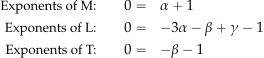
These simultaneous equations have the solution that , and . Therefore, the first product can be written as
![\[ \Pi_1 = \varrho^{-1} \, V_{\rm av}^{-1} \, d^{-1} \mu = \frac{\mu}{\varrho \, V_{\rm av} \, d} \]](https://eaglepubs.erau.edu/app/uploads/quicklatex/quicklatex.com-4dc690642e4db0cb4554a37cdb511aec_l3.svg "Rendered by QuickLaTeX.com")
which is the reciprocal of the Reynolds number, but as discussed before, this grouping can also be inverted to get the first product as the recognizable Reynolds number, i.e.,
![\[ \Pi_1 = \frac{\varrho \, V_{\rm av} \, d}{\mu} = Re \]](https://eaglepubs.erau.edu/app/uploads/quicklatex/quicklatex.com-b0946669e8546d1cec49a463806fee64_l3.svg "Rendered by QuickLaTeX.com")
For the second product then
![\[ \Pi_2 = \varrho^\alpha \, V_{\rm av}^\beta \, d^\gamma \, \epsilon \]](https://eaglepubs.erau.edu/app/uploads/quicklatex/quicklatex.com-744c3fe72d2290c46167427edf1a99be_l3.svg "Rendered by QuickLaTeX.com")
and in terms of dimensions, then
![\[ \left[ \Pi_2 \right] = (\rm ML^{-3})^\alpha \, \rm (LT^{-1})^\beta \, (\rm L)^\gamma \, L =\rm M^0 L^0 T^0 = 1 \]](https://eaglepubs.erau.edu/app/uploads/quicklatex/quicklatex.com-108688c954d0b962b338ab7363da6580_l3.svg "Rendered by QuickLaTeX.com")
and the exponents , and can be reused for convenience. Making the equation dimensionally homogeneous by equating the exponents for each of the dimensions, in turn, gives
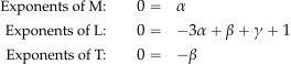
These simultaneous equations have the solution that ,  and . Therefore, the second product can be written as
![\[ \Pi_2 = d^{-1} \, \epsilon = \frac{\epsilon}{d} \]](https://eaglepubs.erau.edu/app/uploads/quicklatex/quicklatex.com-52b40fee0666700e388741baeda89b9a_l3.svg "Rendered by QuickLaTeX.com")
which is a measure of the relative surface roughness.
Finally, for the third product, then
![\[ \Pi_3 = \varrho^\alpha \, V_{\rm av}^\beta \, d^{\gamma} \, dp/dx \]](https://eaglepubs.erau.edu/app/uploads/quicklatex/quicklatex.com-aa33d2b1dbf889dce516b8155464664f_l3.svg "Rendered by QuickLaTeX.com")
and in terms of dimensions, then
![\[ \left[ \Pi_3 \right] = (\rm ML^{-3})^\alpha \, (\rm LT^{-1})^\beta \, (L)^\gamma \rm ML^{-2}T^{-2} = \rm M^0 L^0 T^0 = 1 \]](https://eaglepubs.erau.edu/app/uploads/quicklatex/quicklatex.com-8e41ec341dea82bd933c41dd82b2c979_l3.svg "Rendered by QuickLaTeX.com")
Making the equation dimensionally homogeneous by equating the exponents for each of the dimensions, in turn, gives
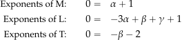
These simultaneous equations have the solution that ,  and . Therefore, the third product can be written as
![\[ \Pi_3 = \varrho^{-1} \, V_{\rm av}^{-2} \, d \, (dp/dx) = \frac{d \, (dp/dx)}{\varrho \, V^2} \]](https://eaglepubs.erau.edu/app/uploads/quicklatex/quicklatex.com-b490a41971fa5be5675cb2076db4edaa_l3.svg "Rendered by QuickLaTeX.com")
which is a dimensionless pressure drop or “head” drop. Usually, this latter grouping is expressed in terms of a friction factor, i.e.,
![\[ f = \frac{d \, (dp/dx)}{\frac{1}{2} \varrho \, V_{\rm av}^2} \]](https://eaglepubs.erau.edu/app/uploads/quicklatex/quicklatex.com-6e9a2b87775d54760b6b24b83cb49418_l3.svg "Rendered by QuickLaTeX.com")
Therefore, the final result is
![\[ f = \phi_1 \left( Re, \, \frac{\epsilon}{d} \right) \]](https://eaglepubs.erau.edu/app/uploads/quicklatex/quicklatex.com-8cad623ffdcbe8638aa40d0feeab8593_l3.svg "Rendered by QuickLaTeX.com")
This result shows that the frictional pressure drop along the pipe will be a function of the Reynolds number and the pipe’s effective dimensionless roughness.
Worked Example #15
The drag on the hull of a ship, , can be written in a general functional form as
![\[ D = f \left( \varrho, \, V, \, l, \, g \right) \]](https://eaglepubs.erau.edu/app/uploads/quicklatex/quicklatex.com-cd47010d3f83365ab73495796ff222af_l3.svg "Rendered by QuickLaTeX.com")
where is the density of the water, is the ship’s speed through the water, and  is a length scale associated with the hull.
Use the Buckingham method to show that
![\[ C_D = \psi (Fr) \]](https://eaglepubs.erau.edu/app/uploads/quicklatex/quicklatex.com-efb3e8de023dfb1d280595ed91afcc55_l3.svg "Rendered by QuickLaTeX.com")
where is a drag coefficient and the dimensionless grouping  is known as the Froude number.
For this problem, the drag can be written as
![\[ D = \phi \left( \varrho, \, V, \, l, \, g \right) \]](https://eaglepubs.erau.edu/app/uploads/quicklatex/quicklatex.com-e03c0f9af5ca7a5f24368f7fb3fe13fb_l3.svg "Rendered by QuickLaTeX.com")
In implicit form, then
![\[ \phi_1 \left( \varrho, \, V, \, l, \, g, \, D \right) = 0 \]](https://eaglepubs.erau.edu/app/uploads/quicklatex/quicklatex.com-471e4895ca6f6cdf9795fb9db62d825e_l3.svg "Rendered by QuickLaTeX.com")
So,  and
and  , so there will be two products.
Setting up the dimensional matrix gives
![\[ \begin{array}{l|r|r|r|r|r} \mbox{\small Base~unit} & \varrho & V & l & g & D \\ \hline \text{\small Mass M:} \quad & 1 & 0 & 0 & 0 & 1 \\ \text{\small Length L:} \quad & -3 & 1 & 1 & 1 & 1 \\ \text{\small Time T:} \quad & 0 & -1 & 0 & -2 & -2 \end{array} \]](https://eaglepubs.erau.edu/app/uploads/quicklatex/quicklatex.com-496389b9783a15da5020b81520bf0c9e_l3.svg "Rendered by QuickLaTeX.com")
Now, the repeating variable must be chosen, for which the standard choice is , , and , which will all primarily influence drag. They also collectively include all of the fundamental dimensions of mass, length, and time. Finding the determinant of the dimensional submatrix that is formed by the repeating variables shows that
![\[ \det \begin{bmatrix} 0 & 0 & 1 \\ 1 & 1 & -3 \\ 0 & -1 & 0 \end{bmatrix} \ne 0 \]](https://eaglepubs.erau.edu/app/uploads/quicklatex/quicklatex.com-ee7e10a2b7dd4473c25a11d07f69a019_l3.svg "Rendered by QuickLaTeX.com")
so the selected repeating variables are linearly independent.
For the first product, then
![\[ \Pi_{1} = \phi_2 \left(l, \, V, \, \varrho, \, g \right) \]](https://eaglepubs.erau.edu/app/uploads/quicklatex/quicklatex.com-bfa71d6b46573bcd9df5248f04ebd4c1_l3.svg "Rendered by QuickLaTeX.com")
and for the second product then
![\[ \Pi_{2} = \phi_3 \left(l, \, V, \, \varrho, \, D \right) \]](https://eaglepubs.erau.edu/app/uploads/quicklatex/quicklatex.com-356e0f8d7f39eeaa66832bc86427c554_l3.svg "Rendered by QuickLaTeX.com")
Continuing with the first product then
![\[ \Pi_{1} = (l)^{\alpha} \, (V)^{\beta}\, (\varrho)^{\gamma} \, g \]](https://eaglepubs.erau.edu/app/uploads/quicklatex/quicklatex.com-eaab97dda2cd1f2722fc31f2c9a05539_l3.svg "Rendered by QuickLaTeX.com")
and in terms of the dimensions, then
![\[ \left[ \Pi_{1} \right] = \rm M^{0}L^{0}T^{0} = (\rm L)^{\alpha} (\rm L T^{-1} )^{\beta} (\rm M L^{-3} )^{\gamma} \rm L T^{-2} \]](https://eaglepubs.erau.edu/app/uploads/quicklatex/quicklatex.com-20b37eaa58b7db21c1e3bbaf9c9a66c8_l3.svg "Rendered by QuickLaTeX.com")
For to be dimensionless, then
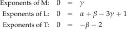
Therefore, = -2, = 0, and  , so the product is
![\[ \Pi_1 = (l)^{1}\, (V)^{-2} \, (\varrho)^{0} \, g \]](https://eaglepubs.erau.edu/app/uploads/quicklatex/quicklatex.com-a6bececaa49537a726f806970952c458_l3.svg "Rendered by QuickLaTeX.com")
or
![\[ \Pi_1 = \frac{l g}{V^2} \quad \mbox{or} \quad \frac{V^2}{l g} \quad \mbox{or} \quad \frac{V}{\sqrt{l \, g}} \]](https://eaglepubs.erau.edu/app/uploads/quicklatex/quicklatex.com-6d3d012461a38d739079b464d90e8c51_l3.svg "Rendered by QuickLaTeX.com")
which is the Froude number,  .
.
For the second product then
![\[ \Pi_{2} = (l)^{\alpha}\, (V)^{\beta} \, (\varrho)^{\gamma} \, D \]](https://eaglepubs.erau.edu/app/uploads/quicklatex/quicklatex.com-b123248988d7802b5da1917cee437e89_l3.svg "Rendered by QuickLaTeX.com")
and in terms of the dimensions, then
![\[ \left[ \Pi_{2} \right] = \rm M^{0}L^{0}T^{0} = (\rm L)^{\alpha} (\rm L T^{-1} )^{\beta} (\rm M L^{-3} )^{\gamma} \rm M L T^{-2} \]](https://eaglepubs.erau.edu/app/uploads/quicklatex/quicklatex.com-75c56505af225e4504da8db6efd1ae30_l3.svg "Rendered by QuickLaTeX.com")
For  to be dimensionless, then
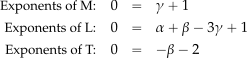
Therefore, = -2, = -1, and  , so the product is
![\[ \Pi_2 = (l)^{-2}\, (V)^{-2}\, (\varrho)^{-1} \, D \]](https://eaglepubs.erau.edu/app/uploads/quicklatex/quicklatex.com-018106ad0d9d6ea3d1612eee6b0ebee8_l3.svg "Rendered by QuickLaTeX.com")
or
![\[ \Pi_2 = \frac{D}{\varrho l^2 \, V^2} \]](https://eaglepubs.erau.edu/app/uploads/quicklatex/quicklatex.com-da7597807b4b1af07d88eef6f95e007c_l3.svg "Rendered by QuickLaTeX.com")
which is a drag coefficient, .
Therefore, the final result is
i.e., the drag coefficient on the hull is some function of the Froude number.
Worked Example #16
A tiny spherical particle of diameter falls freely vertically at velocity in the atmosphere. The aerodynamic drag on the particle  can be written in general functional form as
![\[ {\cal{D}} = f( D, \, V, \, \mu ) \]](https://eaglepubs.erau.edu/app/uploads/quicklatex/quicklatex.com-2fd4dc3a1e8f4d4ecd3c8f6d66ed4e7d_l3.svg "Rendered by QuickLaTeX.com")
where  is the function to be determined and is the coefficient of viscosity. Using the Buckingham method, find the dimensionless similarity parameter that governs this freely falling behavior.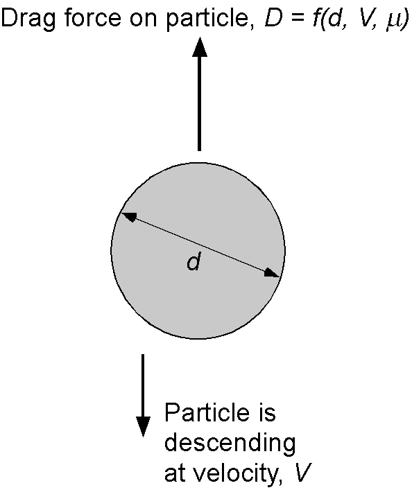
The information given is that
![\[ {\cal{D}} = f( D, \, V, \, \mu ) \]](https://eaglepubs.erau.edu/app/uploads/quicklatex/quicklatex.com-c591b8dff579a2dddfd3f68b2f0bad0d_l3.svg "Rendered by QuickLaTeX.com")
So, in implicit form, then
![\[ \phi_1 (D, \, V, \mu, \, {\cal{D}} ) = 0 \]](https://eaglepubs.erau.edu/app/uploads/quicklatex/quicklatex.com-83f50794d5eaf13e21a285c0207141fa_l3.svg "Rendered by QuickLaTeX.com")
Therefore,  and (by inspection, mass, length, and time are all involved in this problem), so there is just one product. Setting down the dimensional matrix gives
![\[ \begin{array}{l|r|r|r|r|r} \mbox{\small Base~unit} & D & V & \mu & {\cal{D}} \\ \hline \text{\small Mass M:} \quad & 0 & 0 & 1 & 1 \\ \text{\small Length L:} \quad & 1 & 1 & -1 & 1 \\ \text{\small Time T:} \quad & 0 & -1 & -1 & -2 \end{array} \]](https://eaglepubs.erau.edu/app/uploads/quicklatex/quicklatex.com-e1c11c74579b7189bec54981c1f62704_l3.svg "Rendered by QuickLaTeX.com")
For the product, then
![\[ \Pi = (D)^{\alpha} \, (V)^{\beta} \, (\mu)^{\gamma} \, {\cal{D}} \]](https://eaglepubs.erau.edu/app/uploads/quicklatex/quicklatex.com-4fef3a0793033882719248cb0072a780_l3.svg "Rendered by QuickLaTeX.com")
and in terms of dimensions, then
![\[ \left[ \Pi \right] = \rm M^{0}L^{0}T^{0} = (\rm L)^{\alpha} (\rm L T^{-1})^{\beta} (M L^{-1} \rm T^{-1})^{\gamma} \rm M L T^{-2} \]](https://eaglepubs.erau.edu/app/uploads/quicklatex/quicklatex.com-fa202f25f9abf73c705093f210981aa5_l3.svg "Rendered by QuickLaTeX.com")
For to be dimensionless, then
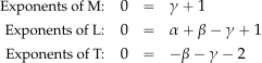
and so = -1, and and = -1.
Therefore, the product is
![\[ \Pi = (D)^{-1} \, (V)^{-1} \, (\mu)^{-1} \, {\cal{D}} = \frac{{\cal{D}}}{D \, V \mu} \]](https://eaglepubs.erau.edu/app/uploads/quicklatex/quicklatex.com-13153e6a1cc024c19649baab0bdc72fc_l3.svg "Rendered by QuickLaTeX.com")
which is a viscous drag coefficient applicable, in this case, to what is known as a Stokes flow, which is a flow corresponding to Reynolds numbers near unity.
Worked Example #17
A flow experiment with a circular cylinder shows that at a specific condition, a vortex shedding phenomenon at frequency appears in the wake downstream of the cylinder.
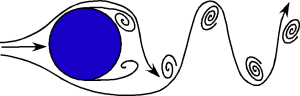 Use dimensional analysis to show that the dimensionless parameter that governs this process, known as a Strouhal number
  , is given by
![\[ St = \frac{ f \, d}{V} \]](https://eaglepubs.erau.edu/app/uploads/quicklatex/quicklatex.com-31f822f591dcf9919ceea82c4c036927_l3.svg "Rendered by QuickLaTeX.com")
where is the flow speed and is the diameter of the cylinder.
The frequency of shedding is assumed to be a function of the diameter of the cylinder and flow velocity . Working with this information, then
![\[ f = \phi \left( d, \, V \right) \]](https://eaglepubs.erau.edu/app/uploads/quicklatex/quicklatex.com-252e4682f72d544e9dede8882b6eb408_l3.svg "Rendered by QuickLaTeX.com")
or in the implicit form, then
![\[ \phi_1 \left( d, \, V , \, f \right) = 0 \]](https://eaglepubs.erau.edu/app/uploads/quicklatex/quicklatex.com-83326c3e1a26dd397e9ecdcce004cf0e_l3.svg "Rendered by QuickLaTeX.com")
Therefore,  , but in this case,
  because only length and time are involved in this group of variables (no mass). So, there is just one product to determine.
Setting up the dimensional matrix, i.e.,
![\[ \begin{array}{l|r|r|r|} \mbox{\small Base~unit} & d & V & f \\ \hline \text{\small Length L:} \quad & 1 & 1 & 0 \\ \text{\small Time T:} \quad & 0 & -1 & -1 \end{array} \]](https://eaglepubs.erau.edu/app/uploads/quicklatex/quicklatex.com-b646919467860144e6563ca5e30fe2b8_l3.svg "Rendered by QuickLaTeX.com")
So, the first grouping is
![\[ \Pi_{1} = (d)^{\alpha} \, (V)^{\beta} \, f \]](https://eaglepubs.erau.edu/app/uploads/quicklatex/quicklatex.com-30dc40dccfd86071bb09f7e695e3363f_l3.svg "Rendered by QuickLaTeX.com")
and in terms of the dimensions, then
![\[ \left[ \Pi_{1} \right] = \rm M^{0}L^{0}T^{0} = (\rm L)^{\alpha} (\rm L T^{-1} )^{\beta} \rm T^{-1} \]](https://eaglepubs.erau.edu/app/uploads/quicklatex/quicklatex.com-43eee8296c59b3e56a1a06a56ece0900_l3.svg "Rendered by QuickLaTeX.com")
For to be dimensionless, then
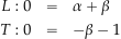
Therefore, = -1 and , so the product is
![\[ \Pi_1 = (d)^{1}(V)^{-1} f = \frac{f \, d}{V} \]](https://eaglepubs.erau.edu/app/uploads/quicklatex/quicklatex.com-569b2d85d4c34bd0c3fb48fbdbef3247_l3.svg "Rendered by QuickLaTeX.com")
which is the Strouhal number , as called for in the question.
A result could also have been obtained by recognizing that the frequency of shedding may also be a function of the flow density and its viscosity . In this case, there is a strong expectation that the Reynolds number may be involved. In this case, then
![\[ f = \phi \left( d, \, V , \, \varrho, \, \mu \right) \]](https://eaglepubs.erau.edu/app/uploads/quicklatex/quicklatex.com-e08074b7ac381bc2af1b88f95f64fd4e_l3.svg "Rendered by QuickLaTeX.com")
or in the implicit form, then
![\[ \phi_1 \left( d, \, V , \varrho, \, \mu \, f \right) = 0 \]](https://eaglepubs.erau.edu/app/uploads/quicklatex/quicklatex.com-cca623fcb7457d6b09f6621794ee7ec8_l3.svg "Rendered by QuickLaTeX.com")
In this case, and (mass is now involved), so there are two products to determine. Of course, there is an expectation that one of these has already been determined.
Setting up the dimensional matrix gives
![\[ \begin{array}{l|r|r|r|r|r} \mbox{\small Base~unit} & d & V & \varrho & \mu & f \\ \hline \text{\small Mass M:} \quad & 0 & 0 & 0 & 1 & 0 \\ \text{\small Length L:} \quad & 1 & 1 & 1 & -1 & 0 \\ \text{\small Time T:} \quad & 0 & -1 & -3 & -1 & -1 \end{array} \]](https://eaglepubs.erau.edu/app/uploads/quicklatex/quicklatex.com-96fe4437378b45e1ec6afe71767b92a4_l3.svg "Rendered by QuickLaTeX.com")
Proceeding as usual with the selection of the repeating variables (again, the standard choice is , , and ), then
![\[ \Pi_{1} = \phi_2 \left(d, \, V, \, \varrho, \, f \right) \]](https://eaglepubs.erau.edu/app/uploads/quicklatex/quicklatex.com-7e72f1355ef7758b8e59dd320a418b4d_l3.svg "Rendered by QuickLaTeX.com")
and
![\[ \Pi_{2} = \phi_3 \left(d, \, V, \, \varrho, \, \mu \right) \]](https://eaglepubs.erau.edu/app/uploads/quicklatex/quicklatex.com-22428adf49655c3991da040b9481cdea_l3.svg "Rendered by QuickLaTeX.com")
For the first product then
![\[ \Pi_{1} = (d)^{\alpha} \, (V)^{\beta} \, (\varrho)^{\gamma} \, f \]](https://eaglepubs.erau.edu/app/uploads/quicklatex/quicklatex.com-0856d9e87c680693654c2863b4985177_l3.svg "Rendered by QuickLaTeX.com")
and terms of the dimensions, then
![\[ \left[ \Pi_{1} \right] = \rm M^{0}L^{0}T^{0} = (\rm L)^{\alpha} (\rm L T^{-1} )^{\beta} (\rm M L^{-3} )^{\gamma} \rm T^{-1} \]](https://eaglepubs.erau.edu/app/uploads/quicklatex/quicklatex.com-37d957e5b374529ca3f98091ed158afe_l3.svg "Rendered by QuickLaTeX.com")
For to be dimensionless, then
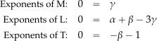
Therefore, = -1, = 0, and , so the product is
![\[ \Pi_1 = (d)^{1}(V)^{-1} f = \frac{f d}{V} \]](https://eaglepubs.erau.edu/app/uploads/quicklatex/quicklatex.com-e50d01748e488c8dae66f71b76d36150_l3.svg "Rendered by QuickLaTeX.com")
which is the Strouhal number , as derived previously.
For the second product, which is suspected to be a Reynolds number, then
![\[ \Pi_{2} = (d)^{\alpha} \, (V)^{\beta} \, (\varrho)^{\gamma} \, \mu \]](https://eaglepubs.erau.edu/app/uploads/quicklatex/quicklatex.com-e6844120790bf5d0d66c19740e7ec54c_l3.svg "Rendered by QuickLaTeX.com")
and terms of the dimensions, then
![\[ \left[ \Pi_{2} \right] = \rm M^{0}L^{0}T^{0} = (\rm L)^{\alpha} (\rm L T^{-1} )^{\beta} (\rm M L^{-3} )^{\gamma} \rm M L^{-1} T^{-1} \]](https://eaglepubs.erau.edu/app/uploads/quicklatex/quicklatex.com-b386f36870e0574014d58f4d4789591f_l3.svg "Rendered by QuickLaTeX.com")
For to be dimensionless, then
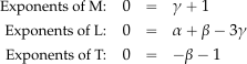
Therefore, = -1, = -1, and , so the product is
![\[ \Pi_2 = (d)^{-1} \, (V)^{-1} \, (\varrho)^{-1}\, \mu = \frac{\mu }{\varrho \, V \, d} \quad \mbox{or} \quad \frac{\varrho \, V \, d}{\mu } \]](https://eaglepubs.erau.edu/app/uploads/quicklatex/quicklatex.com-deabe6996124665f4690b4e594b70dd5_l3.svg "Rendered by QuickLaTeX.com")
which is the Reynolds number  .
.
Therefore, the frequency of shedding is expected to be a function of Reynolds number, i.e.,
![\[ St = \phi_4 ( Re ) \]](https://eaglepubs.erau.edu/app/uploads/quicklatex/quicklatex.com-b9333814af44ddeaa3c02939ac3d3e9b_l3.svg "Rendered by QuickLaTeX.com")
Worked Example #18
Define the Reynolds number and explain its meaning. Show that the Reynolds number represents a ratio of the relative magnitude of inertial effects to viscous effects in the flow. Hint: Multiply both the numerator and denominator of the equation for the Reynolds number by a velocity and a length scale.
The Reynolds number is a dimensionless grouping formed in terms of fluid density, , a reference velocity, , a characteristic length scale, , and viscosity, , i.e.,
![\[ Re = \frac{\varrho \, V \, L}{\mu} \]](https://eaglepubs.erau.edu/app/uploads/quicklatex/quicklatex.com-d0adee81a14404d3db86863400178405_l3.svg "Rendered by QuickLaTeX.com")
The Reynolds number represents “the ratio of the relative effects of inertial effects to viscous effects,” which can be seen by writing
![\[ Re = \frac{\varrho_{\infty} \, V_{\infty} \, c}{\mu_{\infty}} = \frac{\varrho_{\infty} \, V_{\infty} \, c (V_{\infty} \, c)}{\mu_{\infty} \, (V_{\infty} c)} = \frac{\varrho_{\infty} \, V_{\infty}^2 \, c^2}{\mu_{\infty} (V_{\infty}/c) c^2} \equiv \frac{\mbox{\small Inertial force}}{\mbox{\small Viscous force}} \]](https://eaglepubs.erau.edu/app/uploads/quicklatex/quicklatex.com-dbdd708aead8360204cfd41c3a76146e_l3.svg "Rendered by QuickLaTeX.com")
On the numerator,  has units of force, representing an inertial force, i.e.,
![\[ \left[ \varrho_{\infty} \, V_{\infty}^2 \, c^2 \right] = \rm M L^{-3} L^2 T^{-2} L^2 = \rm M L T^{-2} \]](https://eaglepubs.erau.edu/app/uploads/quicklatex/quicklatex.com-480baef05bb8e7ba1a8712ce7409ecc7_l3.svg "Rendered by QuickLaTeX.com")
The coefficient of viscosity, , is the shear force per unit area per unit velocity gradient, i.e., Newton’s law of viscosity, so the denominator is also a force, but a viscous force. Hence, the significance of the Reynolds number becomes apparent as a relative measure of inertial effects to viscous effects in a fluid flow.
Worked Example #19
The distance traveled by a dimpled golf ball depends on its aerodynamic drag,  , which in turn on its flight speed , the density of the air , the viscosity of the air , the diameter of the ball , and the diameter of the dimples on the ball , i.e., =
  (, , , , ), where is some functional dependency. Use dimensional analysis (Buckingham method) to determine the dimensionless groupings that govern this problem.
The drag of the golf ball (the dependent variable) can be written in a functional form as
![\[ {\cal{D}} = \phi (V, \, \varrho, \, \mu, \, D, \, d) \]](https://eaglepubs.erau.edu/app/uploads/quicklatex/quicklatex.com-16f3ab617e3d845b84c9a289011dd819_l3.svg "Rendered by QuickLaTeX.com")
where is a function to be determined. This equation can be written in an implicit form as
![\[ \phi_1(V, \varrho, \, \mu, \, D, \, d, \, {\cal{D}}) = 0 \]](https://eaglepubs.erau.edu/app/uploads/quicklatex/quicklatex.com-45ecf7624ec94f8957f6a354d2af03f8_l3.svg "Rendered by QuickLaTeX.com")
In this case, there are six variables () and three fundamental dimensions (), so there are three products.
The functional dependence can also be written in the form
![\[ \phi_2 (\Pi_1, \, \Pi_2, \, \Pi_3) = 0 \]](https://eaglepubs.erau.edu/app/uploads/quicklatex/quicklatex.com-5ce51229be9ed4bb525446e1e090b8c1_l3.svg "Rendered by QuickLaTeX.com")
where , and are the dimensionless groupings to be determined.
Choose the standard aerodynamic repeating variables , , and , which are all linearly independent. This result can be confirmed by finding the determinant of the dimensional submatrix that is formed by the repeating variables, which shows that
so the selected repeating variables are linearly independent.
The dimensionless products can each be written in terms of these repeating variables plus one other variable, that is
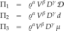
where in each case the values of the exponents , , and are to be determined so that each of the products is dimensionless.
For this problem, then
![\begin{eqnarray*} \left[ V \right] & = & \rm L T^{-1} \\ \left[ \varrho \right] & = & \rm M L^{-3} \\ \left[ \mu \right] & = & \rm M L^{-1} T^{-1} \\ \left[ D \right] & = & \rm L \\ \left[ d \right] & = & \rm L \\ \left[ \cal{D} \right] & = & \rm M L T^{-2} \end{eqnarray*}](https://eaglepubs.erau.edu/app/uploads/quicklatex/quicklatex.com-c61856c7bc032be21d67d2529e073175_l3.svg "Rendered by QuickLaTeX.com")
and so the dimensional matrix is
![\[ \begin{array}{l|r|r|r|r|r|r} \mbox{\small Base~unit} & V & \varrho & \mu & D & d & {\cal{D}} \\ \hline \text{\small Mass M:} & 0 & 1 & 1 & 0 & 0 & 1 \\ \text{\small Length L:} & 1 & -3 & -1 & 1 & 1 & 1 \\ \text{\small Time T:} & -1 & 0 & -1 & 0 & 0 & -2 \end{array} \]](https://eaglepubs.erau.edu/app/uploads/quicklatex/quicklatex.com-8fa28304974c931f00d87f05ccd484ea_l3.svg "Rendered by QuickLaTeX.com")
Considering the first product then
![\[ \left[ \Pi_1 \right] = \varrho^\alpha \, V^\beta \, D^\gamma \, {\cal{D}} \]](https://eaglepubs.erau.edu/app/uploads/quicklatex/quicklatex.com-0b36859491ee7de75f6849c50567a7d9_l3.svg "Rendered by QuickLaTeX.com")
and in terms of dimensions, then
![\[ \left[ \Pi_1 \right] = (\rm M L^{-3})^\alpha (\rm L T^{-1})^\beta (\rm L)^\gamma (\rm M L T^{-2}) = \rm M^0 L^0 T^0 \]](https://eaglepubs.erau.edu/app/uploads/quicklatex/quicklatex.com-177efbe81ae121762291f80dbf0cb9a0_l3.svg "Rendered by QuickLaTeX.com")
Making the equation dimensionally homogeneous by equating the exponents for each of the dimensions, in turn, gives
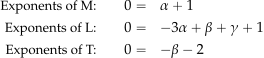
These simultaneous equations have the solution that , and . Therefore, the first product can be written as
![\[ \Pi_1 = \varrho^{-1} \, V^{-2} \, D^{-2} \, {\cal{D}} = \frac{ {\cal{D}} }{\varrho \, V^{2} \, D^{2}} \]](https://eaglepubs.erau.edu/app/uploads/quicklatex/quicklatex.com-56a37322201017b1500fe495bafeecba_l3.svg "Rendered by QuickLaTeX.com")
which is a force coefficient.
Considering the second product then
![\[ \left[ \Pi_2 \right] = \varrho^\alpha \, V^\beta \, D^\gamma \, d \]](https://eaglepubs.erau.edu/app/uploads/quicklatex/quicklatex.com-2735039987ef68b9bbc6798cbc5d2c86_l3.svg "Rendered by QuickLaTeX.com")
and in terms of dimensions, then
![\[ \left[ \Pi_2 \right] = (\rm M L^{-3})^\alpha (\rm L T^{-1})^\beta (L)^\gamma (\rm L) = \rm M^0 L^0 T^0 \]](https://eaglepubs.erau.edu/app/uploads/quicklatex/quicklatex.com-40dc3d1559760f24bf596a4154c0aa5b_l3.svg "Rendered by QuickLaTeX.com")
Making the equation dimensionally homogeneous by equating the exponents for each of the dimensions, in turn, gives
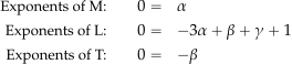
These simultaneous equations have the solution that  ,
,  , and
, and  . Therefore, the second product can be written as
![\[ \Pi_2 = \varrho^{0} \, V^{0} \, D^{-1} \, d = \frac{d}{D} \]](https://eaglepubs.erau.edu/app/uploads/quicklatex/quicklatex.com-654d50763f47a722ea54b4329f2122b3_l3.svg "Rendered by QuickLaTeX.com")
which is a dimensionless length scale, i.e., the ratio of the diameter of the dimples to the diameter of the golf ball.
Considering the third product then
![\[ \Pi_3 = \varrho^\alpha \, V^\beta \, D^\gamma \, \mu \]](https://eaglepubs.erau.edu/app/uploads/quicklatex/quicklatex.com-395802eb0a5868003c01c7f5f9f633fe_l3.svg "Rendered by QuickLaTeX.com")
and in terms of dimensions, then
![\[ \left[ \Pi_3 \right] = (\rm M L^{-3})^\alpha (\rm L T^{-1})^\beta (\rm L)^\gamma (\rm M L^{-1} T^{-1} ) = \rm M^0 L^0 T^0 \]](https://eaglepubs.erau.edu/app/uploads/quicklatex/quicklatex.com-2c128ebe7b5e84ae89f691aed53ac7ac_l3.svg "Rendered by QuickLaTeX.com")
Making the equation dimensionally homogeneous by equating the exponents for each of the dimensions, in turn, gives
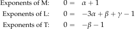
These simultaneous equations have the solution that , and . Therefore, the third product can be written as
![\[ \Pi_3 = \varrho^{-1} \, V^{-1} \, D^{-1} \, \mu = \frac{\mu }{\varrho \, V \, D} \]](https://eaglepubs.erau.edu/app/uploads/quicklatex/quicklatex.com-3f6b0e7a7d2e04b0aa03002a353533e6_l3.svg "Rendered by QuickLaTeX.com")
or inverting the grouping (it is still dimensionless)
![\[ \Pi_3 = \frac{\varrho V \, D}{\mu} \]](https://eaglepubs.erau.edu/app/uploads/quicklatex/quicklatex.com-c4c1b7f421e2461e812e80450085bf96_l3.svg "Rendered by QuickLaTeX.com")
which is a Reynolds number.
Finally, then
![\[ \phi_2 (\Pi_1, \Pi_2, \Pi_3) = \phi_2 \left( \frac{ {\cal{D}} }{\varrho V^{2} D^{2}}, \, \frac{d}{D}, \, \frac{\varrho V D}{\mu} \right) = 0 \]](https://eaglepubs.erau.edu/app/uploads/quicklatex/quicklatex.com-f22200e94f44413e5289ef374c7e75ca_l3.svg "Rendered by QuickLaTeX.com")
or just
![\[ \frac{ {\cal{D}} }{\varrho \, V^{2} \, D^{2}} = \phi_3 \left( \frac{d}{D}, \, \frac{\varrho V D}{\mu} \right) \]](https://eaglepubs.erau.edu/app/uploads/quicklatex/quicklatex.com-34123e8c6619e791904a4b419ffe2c64_l3.svg "Rendered by QuickLaTeX.com")
Worked Example #20
The sound intensity  from a jet engine is found to be a function of the sound pressure level
  (dimensions of pressure) and the fluid properties density, , and speed of sound,
  , as well as the distance from the engine to an observer location,
  . Using the Buckingham method, find a relationship for as a function of the other parameters. Show all of your work. Hint: Sound intensity, , is defined as the acoustic power per unit area emanating from a sound source.
The relationship between and the properties listed may be written in a general functional form as
![\[ I = f \left( p, \, \varrho, \, a, \, r \right) \]](https://eaglepubs.erau.edu/app/uploads/quicklatex/quicklatex.com-aad370575c71fc576c31b730eda1f99e_l3.svg "Rendered by QuickLaTeX.com")
or
![\[ g \left( I, \, p, \varrho, \, a, \, r \right) = 0 \]](https://eaglepubs.erau.edu/app/uploads/quicklatex/quicklatex.com-558711b6efae2c387c51016c9c15e617_l3.svg "Rendered by QuickLaTeX.com")
A hint is given that the sound intensity is defined as the acoustic power per unit area, so this is Watts per unit area in SI. Power is the rate of doing work, and so has units of force times displacement per unit time, i.e., when setting up the problem, then
![\[ \left[ I \right] = \left( \rm M L^{2} T^{-3} \right) L^{-2} = \rm MT^{-3} \]](https://eaglepubs.erau.edu/app/uploads/quicklatex/quicklatex.com-3bbaf4d075d3e8b2284e27fc2bc05f2d_l3.svg "Rendered by QuickLaTeX.com")
Also, pressure is force per unit area, so
![\[ \left[ p \right] = \left(\rm M L T^{-2} \right) \rm L^{-2} = \rm M L^{-1} T^{-2} \]](https://eaglepubs.erau.edu/app/uploads/quicklatex/quicklatex.com-591974b918f3f4c719151fab711f3f77_l3.svg "Rendered by QuickLaTeX.com")
In this problem, and (by inspection, mass, length, and time are all involved), so there are two products to determine. Setting up the dimensional matrix gives
![\[ \begin{array}{l|r|r|r|r|r} \mbox{\small Base~unit} & I & p & \varrho & a & r \\ \hline \text{\small Mass M:} \quad & 1 & 1 & 1 & 0 & 0 \\ \text{\small Length L:} \quad & 0 & -1 & -3 & 1 & 1 \\ \text{\small Time T:} \quad & -3 & -2 & 0 & -1 & 0 \end{array} \]](https://eaglepubs.erau.edu/app/uploads/quicklatex/quicklatex.com-24c7dcc734f568e2e28392d4e538f7a0_l3.svg "Rendered by QuickLaTeX.com")
Proceeding with selecting the repeating variables, one choice is , , and . Therefore, the two groups are
![\[ \Pi_{1} = \phi_1 \left(\varrho, \, a, \, r, \, I \right) \]](https://eaglepubs.erau.edu/app/uploads/quicklatex/quicklatex.com-e992f0941699cd6caf5e3c1697a3c7ec_l3.svg "Rendered by QuickLaTeX.com")
and
![\[ \Pi_{2} = \phi_2 \left(\varrho,\, a, \, r, \, p \right) \]](https://eaglepubs.erau.edu/app/uploads/quicklatex/quicklatex.com-cccbb38671c892888c665985e397a0ff_l3.svg "Rendered by QuickLaTeX.com")
For the first product then
![\[ \Pi_{1} = (\varrho)^{\alpha} \, (a)^{\beta} \, (r)^{\gamma} I \]](https://eaglepubs.erau.edu/app/uploads/quicklatex/quicklatex.com-f6b78b7e8e59bbc19575ad95119e6f1a_l3.svg "Rendered by QuickLaTeX.com")
and in terms of the dimensions, then
![\[ \left[ \Pi_{1} \right] = \rm M^{0}L^{0}T^{0} = (\rm M L^{-3})^{\alpha} ( \rm LT^{-1})^{\beta} ( \rm L )^{\gamma} \, \rm MT^{-3} \]](https://eaglepubs.erau.edu/app/uploads/quicklatex/quicklatex.com-bd14b5474edca48c2a7b2017640b7fa4_l3.svg "Rendered by QuickLaTeX.com")
For to be dimensionless, then
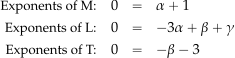
Therefore, , = -3, and = 0, so the product is
![\[ \Pi_1 = (\varrho)^{-1} \, (a)^{-3} \, (r)^0 = \frac{I}{\varrho \, a^3} \]](https://eaglepubs.erau.edu/app/uploads/quicklatex/quicklatex.com-47f6ea97156325594df4b72cf83da4d0_l3.svg "Rendered by QuickLaTeX.com")
For the second product then
![\[ \Pi_{2} = (\varrho)^{\alpha} \, (a)^{\beta} \, (r)^{\gamma} \, p \]](https://eaglepubs.erau.edu/app/uploads/quicklatex/quicklatex.com-080b4db3a5e9822569b57f328934655f_l3.svg "Rendered by QuickLaTeX.com")
and in terms of the dimensions, then
![\[ \left[ \Pi_{2} \right] = \rm M^{0}L^{0}T^{0} = (\rm M L^{-3})^{\alpha} (\rm LT^{-1})^{\beta} (\rm L )^{\gamma} \, \rm M L^{-1} T^{-2} \]](https://eaglepubs.erau.edu/app/uploads/quicklatex/quicklatex.com-1bfb78f36f819096b790510034f98478_l3.svg "Rendered by QuickLaTeX.com")
For to be dimensionless, then
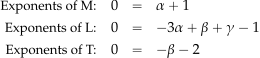
Therefore, , = -2, and = 0, so the product is
![\[ \Pi_2 = (\varrho)^{-1} (a)^{-2} \, (r)^0 \, p = \frac{p}{\varrho \, a^2} \]](https://eaglepubs.erau.edu/app/uploads/quicklatex/quicklatex.com-afcee6d952850abde65ba1da6ec78ec8_l3.svg "Rendered by QuickLaTeX.com")
Interestingly, the factor  is related to the compressibility modulus of the medium in which the sound propagates. Therefore, in this case
![\[ \frac{I}{\varrho a^3}= \phi_4 \left( \frac{p}{\varrho \, a^2} \right) \]](https://eaglepubs.erau.edu/app/uploads/quicklatex/quicklatex.com-9ed365104b811a02b8efee0a9950bd2a_l3.svg "Rendered by QuickLaTeX.com")
Worked Example #21
Consider a liquid in a cylindrical container where both the container and the liquid rotate as a rigid body (called solid-body rotation), as shown in the figure below.
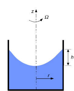 The elevation difference between the center of the liquid surface and the rim of the liquid surface is a function of the angular velocity , the fluid density , the gravitational acceleration , and the radius . Use the Buckingham method to find the relationship between the height and the other parameters. Show all of your work.
In this problem, the objective is to find the effects of the elevation difference between the center of the liquid surface and the rim of the liquid surface, which is a function of the angular velocity , the fluid density , the gravitational acceleration , and the radius , i.e.,
![\[ h = f \left( \omega, \, \varrho, \, g, \, R \right) \]](https://eaglepubs.erau.edu/app/uploads/quicklatex/quicklatex.com-0fb52eb906105759d7333054139c7604_l3.svg "Rendered by QuickLaTeX.com")
or
![\[ \phi_1 \left( h, \, \omega, \, \varrho, \, g, \, R \right) = 0 \]](https://eaglepubs.erau.edu/app/uploads/quicklatex/quicklatex.com-09f9f92e342f04b09f8ef23dc8fd1331_l3.svg "Rendered by QuickLaTeX.com")
Therefore, and (by inspection, mass, length, and time are all involved), so there are two products to determine. Setting up the dimensional matrix gives
![\[ \begin{array}{l|r|r|r|r|r|} \mbox{\small Base~unit} & h & \omega & \varrho & g & R \\ \hline \text{\small Mass M:} \quad & 0 & 0 & 1 & 0 & 0 \\ \text{\small Length L:} \quad & 1 & 0 & -3 & 1 & 1 \\ \text{\small Time T:} \quad & 0 & -1 & 0 & -2 & 0 \end{array} \]](https://eaglepubs.erau.edu/app/uploads/quicklatex/quicklatex.com-f6b6d8f56319e3f694e27c82568526dd_l3.svg "Rendered by QuickLaTeX.com")
Proceeding with selecting the repeating variables, one choice is , , and . Finding the determinant of the dimensional submatrix that is formed by the repeating variables shows that
![\[ \det \begin{bmatrix} 1 & 0 & 0 \\ -3 & 1 & 1 \\ 0 & -2 & 0 \end{bmatrix} \ne 0 \]](https://eaglepubs.erau.edu/app/uploads/quicklatex/quicklatex.com-1dd3b6a51183d74dd8af87c6d7b03f21_l3.svg "Rendered by QuickLaTeX.com")
so the selected repeating variables are linearly independent.
Therefore, the two groups are
![\[ \Pi_{1} = \phi_1 \left(\varrho, \, g, \, R, \, \omega \right) \]](https://eaglepubs.erau.edu/app/uploads/quicklatex/quicklatex.com-57e023485ddb314b2fe1d91b869ba867_l3.svg "Rendered by QuickLaTeX.com")
and
![\[ \Pi_{2} = \phi_2 \left(\varrho, \, g, \, R, \, h \right) \]](https://eaglepubs.erau.edu/app/uploads/quicklatex/quicklatex.com-c7ce877b6acfee36647b79470e075d27_l3.svg "Rendered by QuickLaTeX.com")
For the first product then
![\[ \Pi_{1} = (\varrho)^{\alpha} \, (g)^{\beta} \, (R)^{\gamma} \, \omega \]](https://eaglepubs.erau.edu/app/uploads/quicklatex/quicklatex.com-06ca65693f4c5cbb2aff47320b6d33aa_l3.svg "Rendered by QuickLaTeX.com")
and in terms of the dimensions, then
![\[ \left[ \Pi_{1} \right] = \rm M^{0}L^{0}T^{0} = (\rm M L^{-3})^{\alpha} (\rm LT^{-2})^{\beta} ( \rm L )^{\gamma} \, \rm T^{-1} \]](https://eaglepubs.erau.edu/app/uploads/quicklatex/quicklatex.com-3fbf8058011fe33409930b4987697246_l3.svg "Rendered by QuickLaTeX.com")
For to be dimensionless, then
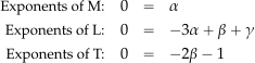
Therefore, , = -1/2, and = 1/2, so the product is
![\[ \Pi_1 = (\varrho)^{0} (g)^{-1/2} (R)^{1/2} \omega = \omega \sqrt{ \frac{R}{g} } \]](https://eaglepubs.erau.edu/app/uploads/quicklatex/quicklatex.com-d4f9066b06b8dcde389f3b9b681d187f_l3.svg "Rendered by QuickLaTeX.com")
For the second product then
![\[ \Pi_{2} = (\varrho)^{\alpha} \, (g)^{\beta} \, (R)^{\gamma} \, h \]](https://eaglepubs.erau.edu/app/uploads/quicklatex/quicklatex.com-262f492e8b230d18f79aded63a87054b_l3.svg "Rendered by QuickLaTeX.com")
and in terms of the dimensions, then
![\[ \left[ \Pi_{2} \right] = \rm M^{0}L^{0}T^{0} = (\rm M L^{-3})^{\alpha} (\rm LT^{-2})^{\beta} (\rm L )^{\gamma} \, \rm L \]](https://eaglepubs.erau.edu/app/uploads/quicklatex/quicklatex.com-269acb7c019cf57939ddfca7b1bd0d86_l3.svg "Rendered by QuickLaTeX.com")
For to be dimensionless, then
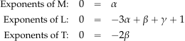
Therefore, , = 0, and = -1, so the product is
![\[ \Pi_2 = (\varrho)^{0} \, (g)^{0} \, (R)^{-1} \, h = \frac{h}{R} \]](https://eaglepubs.erau.edu/app/uploads/quicklatex/quicklatex.com-062a3e602349203820a0bddf7f7d5131_l3.svg "Rendered by QuickLaTeX.com")
Therefore, the final result is
![\[ \frac{h}{R} = \phi_3 \left( \omega \, \sqrt{ \frac{R}{g} } \right) \]](https://eaglepubs.erau.edu/app/uploads/quicklatex/quicklatex.com-91c9708e69c7c46f912934b5a46345ad_l3.svg "Rendered by QuickLaTeX.com")
Worked Example #22
A liquid of density and viscosity flows by gravity through a hole of diameter in the bottom of a tank of diameter . At the start of the experiment, the liquid surface is at a height above the bottom of the tank. The liquid exits the tank as a jet with average velocity straight down. Using the Buckingham method, find a dimensionless relationship for as a function of the other parameters in the problem. Identify any established dimensionless parameters that appear in your result. Show all of your work. Hint: Notice that there are three length scales in this problem, but choose as the reference length scale for consistency.
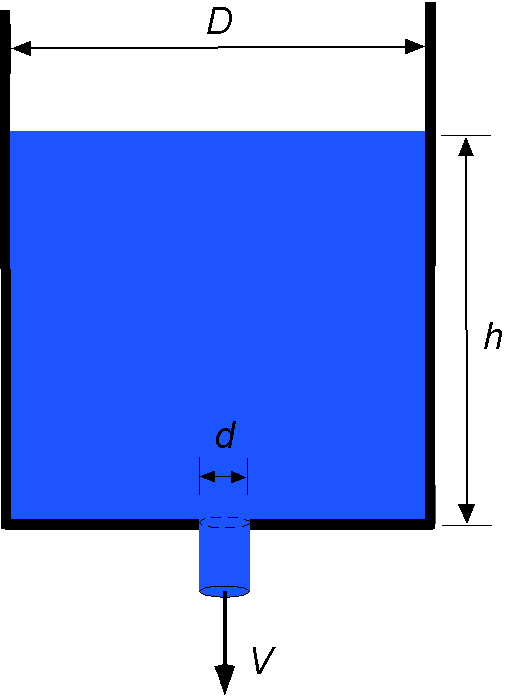
The objective is to find the effects on the exit flow velocity in terms of the fluid density , its viscosity , the diameter of the hole , the diameter of the tank , and the height of the liquid surface , i.e.,
![\[ V = f \left( \varrho, \, \mu, \, d, \, D, \, h \right) \]](https://eaglepubs.erau.edu/app/uploads/quicklatex/quicklatex.com-0512e1a0fac5e0e07b218f0a47a51802_l3.svg "Rendered by QuickLaTeX.com")
or
![\[ \phi_1 \left( V, \, \varrho, \, \mu, \, d, \, D, h \right) = 0 \]](https://eaglepubs.erau.edu/app/uploads/quicklatex/quicklatex.com-ef9af21dd916e91fb6580184cb2f4c2d_l3.svg "Rendered by QuickLaTeX.com")
Therefore, and (by inspection, mass, length, and time are all involved), so there are three products to determine. Setting up the dimensional matrix gives
![\[ \begin{array}{l|r|r|r|r|r|r|} \mbox{\small Base~unit} & V & \varrho & \mu & d & D & h \\ \hline \text{\small Mass M:} \quad & 0 & 1 & 1 & 0 & 0 & 0 \\ \text{\small Length L:} \quad & 1 & -3 & -1 & 1 & 1 & 1 \\ \text{\small Time T:} \quad & -1 & 0 & -1 & 0 & 0 & 0 \end{array} \]](https://eaglepubs.erau.edu/app/uploads/quicklatex/quicklatex.com-fab80e153dabda17d2236e647de4af18_l3.svg "Rendered by QuickLaTeX.com")
Proceeding with selecting the repeating variables, the only choice, in this case, is , , and . Finding the determinant of the dimensional submatrix that is formed by the repeating variables shows that
![\[ \det \begin{bmatrix} 1 & 1 & 0 \\ -3 & -1 & 1 \\ 0 & -1 & 0 \end{bmatrix} \ne 0 \]](https://eaglepubs.erau.edu/app/uploads/quicklatex/quicklatex.com-39c97b4f86a25aeeafc3fca19b221352_l3.svg "Rendered by QuickLaTeX.com")
so the selected repeating variables are linearly independent.
Therefore, the three groups are
![\[ \Pi_{1} = \phi_1 \left(\varrho, \, \mu, \, h, \, V \right) \]](https://eaglepubs.erau.edu/app/uploads/quicklatex/quicklatex.com-b1a1269a960dd642575a47ef6600762f_l3.svg "Rendered by QuickLaTeX.com")
and
![\[ \Pi_{2} = \phi_2 \left( \varrho, \, \mu, \, h, \, d \right) \]](https://eaglepubs.erau.edu/app/uploads/quicklatex/quicklatex.com-58ad2595b5f3e045e7c55acc25b396f3_l3.svg "Rendered by QuickLaTeX.com")
and
![\[ \Pi_{3} = \phi_4 \left( \varrho, \, \mu, \, h, \, D \right) \]](https://eaglepubs.erau.edu/app/uploads/quicklatex/quicklatex.com-f907c0af34d03b41bb61e78ef88a7ebc_l3.svg "Rendered by QuickLaTeX.com")
For the first product then
![\[ \Pi_{1} = (\varrho)^{\alpha} \, (\mu)^{\beta} \, (h)^{\gamma} \, V \]](https://eaglepubs.erau.edu/app/uploads/quicklatex/quicklatex.com-5be8ebfdff2b2fbbdfcc8fd1a4acbf0b_l3.svg "Rendered by QuickLaTeX.com")
and in terms of the dimensions, then
![\[ \left[ \Pi_{1} \right] = \rm M^{0}L^{0}T^{0} = (\rm M L^{-3})^{\alpha} \, (\rm M L^{-1} \, \rm T^{-1})^{\beta} \, ( \rm L )^{\gamma} \, \rm LT^{-1} \]](https://eaglepubs.erau.edu/app/uploads/quicklatex/quicklatex.com-d268b8c201a35adf72aabda3c36d2cf7_l3.svg "Rendered by QuickLaTeX.com")
For to be dimensionless, then
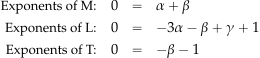
Therefore, = -1, = 1, and = 1, so the product is
![\[ \Pi_1 = (\varrho)^{1} \, (\mu)^{-1} \, (h)^{1} \, V = \frac{\varrho \, V \, h}{\mu} \]](https://eaglepubs.erau.edu/app/uploads/quicklatex/quicklatex.com-e3473b0c9408b6950e549df98351b642_l3.svg "Rendered by QuickLaTeX.com")
which is recognized as a Reynolds number.
For the second product then
![\[ \Pi_{2} = (\varrho)^{\alpha} \, (\mu)^{\beta} (h)^{\gamma} \, d \]](https://eaglepubs.erau.edu/app/uploads/quicklatex/quicklatex.com-6d613989062d0893c8f31e14118b691a_l3.svg "Rendered by QuickLaTeX.com")
and in terms of the dimensions, then
![\[ \left[ \Pi_{2} \right] = \rm M^{0}L^{0}T^{0} = (\rm M L^{-3})^{\alpha} ( \rm M L^{-1}T^{-1})^{\beta} ( \rm L )^{\gamma} \, \rm L \]](https://eaglepubs.erau.edu/app/uploads/quicklatex/quicklatex.com-67a9294c34902e7f44fe46186d9b2db1_l3.svg "Rendered by QuickLaTeX.com")
For to be dimensionless, then
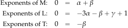
Therefore, = 0, = 0, and = -1, so the product is
![\[ \Pi_2 = (\varrho)^{0} (\mu)^{0} \, (h)^{-1} \, d = \frac{d}{h} \]](https://eaglepubs.erau.edu/app/uploads/quicklatex/quicklatex.com-17febd86d6e1d319c8cdb77e6471b0e4_l3.svg "Rendered by QuickLaTeX.com")
For the third product then
![\[ \Pi_{3} = (\varrho)^{\alpha} \, (\mu)^{\beta} \, (h)^{\gamma} \, D \]](https://eaglepubs.erau.edu/app/uploads/quicklatex/quicklatex.com-4989f9c942f771835256e77ae7971819_l3.svg "Rendered by QuickLaTeX.com")
which quickly follows as per the product as
![\[ \Pi_3 = (\varrho)^{0} \, (\mu)^{0} \, (h)^{-1} \, d = \frac{D}{h} \]](https://eaglepubs.erau.edu/app/uploads/quicklatex/quicklatex.com-205f7be6d4a188c7cba1332a9ba64945_l3.svg "Rendered by QuickLaTeX.com")
Therefore, in this case, the dimensionless groupings involved are such that
![\[ \frac{\varrho \, V \, h}{\mu} = \phi_4 \left( \frac{d}{h}, \, \frac{D}{h} \right) \]](https://eaglepubs.erau.edu/app/uploads/quicklatex/quicklatex.com-4e11f88cbc131b0bb0cdc3cb6a9db77e_l3.svg "Rendered by QuickLaTeX.com")
Worked Example #23
The AIAA Design Build & Fly (DBF) team must determine the factors influencing the aerodynamic drag on a rectangular banner being towed behind their airplane.
 The size of the banner is determined by its length, , and height, . Use the Buckingham method to determine the dimensionless groupings governing this problem. You may also assume that the problem is governed by the airspeed of the airplane, as well as the density and viscosity of the air. Assume further that the banner remains flat and does not flutter in the flow behind the airplane.
The relationship between the drag on the banner and the air properties can be written in the general functional form as
![\[ D = f \left( \varrho_{\infty}, V_{\infty}, \mu_{\infty}, h, l \right) \]](https://eaglepubs.erau.edu/app/uploads/quicklatex/quicklatex.com-06456bb3b92892f49432c20ec37fa337_l3.svg "Rendered by QuickLaTeX.com")
where the size of the banner is represented by its length, , and height, . The functional dependence of in implicit form is
![\[ g \left( \varrho_{\infty}, V_{\infty}, \mu_{\infty}, h, l, D \right) = 0 \]](https://eaglepubs.erau.edu/app/uploads/quicklatex/quicklatex.com-b264b9524dc2da6d59ad39e0b4e63bc6_l3.svg "Rendered by QuickLaTeX.com")
Counting the variables gives and because this problem has three fundamental dimensions. Therefore, , and there will be three products. For each variable, the dimensions are
![\begin{eqnarray*} \left[ D \right] & = & \rm MLT^{-2} \\ \left[ \varrho_{\infty} \right] & = & \rm ML^{-3} \\ \left[ V_{\infty} \right] & = & \rm LT^{-1} \\ \left[ \mu_{\infty} \right] & = & \rm ML^{-1}T^{-1} \\ \left[ h \right] & = & \rm L \\ \left[ l \right] & = & \rm L \end{eqnarray*}](https://eaglepubs.erau.edu/app/uploads/quicklatex/quicklatex.com-fd17beb37e0b8ba8d30da7a973915538_l3.svg "Rendered by QuickLaTeX.com")
The dimensional matrix is
![\[ \begin{array}{l|r|r|r|r|r|r} \mbox{\small Base~unit} & D & \varrho_{\infty} & V_{\infty} & \mu_{\infty} & h & l \\ \hline \text{\small Mass M: } & 1 & 1 & 0 & 1 & 0 & 0 \\ \text{\small Length L: } & 1 & -3 & 1 & -1 & 1 & 1 \\ \text{\small Time T: } & -2 & 0 & -1 & -1 & 0 & 0 \end{array} \]](https://eaglepubs.erau.edu/app/uploads/quicklatex/quicklatex.com-b9efe3d804701de2f7ecb57f666e0b50_l3.svg "Rendered by QuickLaTeX.com")
Choose , , and as the repeating variables, which will all have primary effects on the drag of the banner. These variables also collectively include all the fundamental dimensions of this problem. Finding the determinant of the dimensional submatrix that is formed by the repeating variables shows that
![\[ \det \begin{bmatrix} 1 & 0 & 0 \\ -3 & 1 & 1 \\ 0 & -1 & 0 \end{bmatrix} \ne 0 \]](https://eaglepubs.erau.edu/app/uploads/quicklatex/quicklatex.com-577b40f0ce09e26c72e6c26fcb7785be_l3.svg "Rendered by QuickLaTeX.com")
so the selected repeating variables are linearly independent.
Following the Buckingham method, then the three products are:
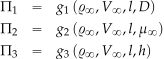
For :
![\[ \Pi_{1} = (\varrho_{\infty})^{\alpha} (V_{\infty})^{\beta} (l)^{\gamma} \, D \]](https://eaglepubs.erau.edu/app/uploads/quicklatex/quicklatex.com-fcd320ee1ca80b32de9307c695920a45_l3.svg "Rendered by QuickLaTeX.com")
The values of the coefficients , , and must now be obtained to make the equation dimensionally homogeneous. In terms of the dimensions of the parameters, then
![\[ \left[ \Pi_{1} \right] = 1 = \rm M^{0}L^{0}T^{0} = \left(\rm ML^{-3} \right)^{\alpha} \left(\rm LT^{-1} \right)^{\beta} \left( \rm L \right)^{\gamma} \left( \rm MLT^{-2} \right) \]](https://eaglepubs.erau.edu/app/uploads/quicklatex/quicklatex.com-ef452984f5c32fa97dffd321d8312979_l3.svg "Rendered by QuickLaTeX.com")
For to be dimensionless, then the powers or exponents of M, L, and T must add to zero, i.e.,
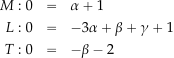
By inspection , , and . Therefore, the first product is
![\[ \Pi_{1} = (\varrho_{\infty})^{\alpha} (V_{\infty})^{\beta} (l)^{\gamma} D = \varrho_{\infty}^{-1} V_{\infty}^{-2} l^{-2} \, D \]](https://eaglepubs.erau.edu/app/uploads/quicklatex/quicklatex.com-0e6bb5a6c3c5e9080950add37694aea6_l3.svg "Rendered by QuickLaTeX.com")
or
![\[ \Pi_{1} = \frac{D}{\varrho_{\infty} V_{\infty}^{2}\ l^2} \]](https://eaglepubs.erau.edu/app/uploads/quicklatex/quicklatex.com-a3b49272563189fe23f0b5356ba09113_l3.svg "Rendered by QuickLaTeX.com")
i.e., a form of the drag coefficient. Aerodynamic force coefficients are usually defined in terms of the dynamic pressure, i.e.,  , so that more conventionally the force coefficient is defined as
![\[ \Pi_{1} = C_D = \frac{D}{ \frac{1}{2} \varrho_{\infty} V_{\infty}^{2} \, l^2} \]](https://eaglepubs.erau.edu/app/uploads/quicklatex/quicklatex.com-5f9ae875e1d7ad6d90b395d5c9ee14dc_l3.svg "Rendered by QuickLaTeX.com")
It would also be legitimate to write the drag coefficient as
![\[ C_D = \frac{D}{ \frac{1}{2} \varrho_{\infty} V_{\infty}^{2} \, l \, h } = \frac{D}{ \frac{1}{2} \varrho_{\infty} V_{\infty}^{2} \, A } \]](https://eaglepubs.erau.edu/app/uploads/quicklatex/quicklatex.com-cbbab83d763c646d97416d4a94d0f623_l3.svg "Rendered by QuickLaTeX.com")
where the banner area  is used rather than
  . Ultimately, how is defined is just a matter of convenience and/or consistency with established conventions. For :
![\[ \Pi_{2} = (\varrho_{\infty})^{\alpha} (V_{\infty})^{\beta} (l)^{\gamma} \, \mu_{\infty} \]](https://eaglepubs.erau.edu/app/uploads/quicklatex/quicklatex.com-f0c2fb6eddc6d314444c234603368edf_l3.svg "Rendered by QuickLaTeX.com")
so
![\[ \left[ \Pi_{2} \right] = 1 = \rm M^{0} L^{0} T^{0} = \left(\rm ML^{-3} \right)^{\alpha} \left( \rm LT^{-1} \right)^{\beta} \left(\rm L\right)^\gamma \left( ML^{-1}T^{-1} \right) \]](https://eaglepubs.erau.edu/app/uploads/quicklatex/quicklatex.com-72b9a117c5ba087a14ae1d90ca3e4561_l3.svg "Rendered by QuickLaTeX.com")
and
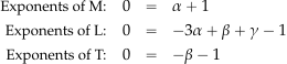
Therefore, in this case , , and , so
![\[ \Pi_{2} = (\varrho_{\infty})^{\alpha} (V_{\infty})^{\beta} (l)^{\gamma} \mu_{\infty} = \varrho_{\infty}^{-1} V_{\infty}^{-1} l^{-1} \, \mu_{\infty} \]](https://eaglepubs.erau.edu/app/uploads/quicklatex/quicklatex.com-b8588c46cf3c78a2216e68e4a09d89ed_l3.svg "Rendered by QuickLaTeX.com")
or
![\[ \Pi_{2} = \frac{\mu_{\infty}}{\varrho_{\infty} V_{\infty} l} \]](https://eaglepubs.erau.edu/app/uploads/quicklatex/quicklatex.com-82026714e5b69b3e08f0e169983e167a_l3.svg "Rendered by QuickLaTeX.com")
Inverting the grouping gives
![\[ \Pi_{2} = \frac{\varrho_{\infty} V_{\infty} l}{\mu_{\infty}} \]](https://eaglepubs.erau.edu/app/uploads/quicklatex/quicklatex.com-c6b5007d34d3f9a230e405fa2d3dd9e0_l3.svg "Rendered by QuickLaTeX.com")
which, in the latter case, is a Reynolds number based on the banner length. Notice that the grouping can be inverted by following established conventions for a similarity parameter or because it is otherwise convenient.
For  :
:
![\[ \Pi_{3} = (\varrho_{\infty})^{\alpha} (V_{\infty})^{\beta} (l)^{\gamma} \, h \]](https://eaglepubs.erau.edu/app/uploads/quicklatex/quicklatex.com-6f9129dbf335bba3a37c113f9004399a_l3.svg "Rendered by QuickLaTeX.com")
so
![\[ \left[ \Pi_{3} \right] = 1 = \rm M^{0}L^{0}T^{0} = \left( \rm ML^{-3} \right)^{\alpha} \left(\rm LT^{-1} \right) ^{\beta} \left( \rm L \right)^{\gamma}\rm L \]](https://eaglepubs.erau.edu/app/uploads/quicklatex/quicklatex.com-09a1f83f0c7a631fbfe2346a444515c6_l3.svg "Rendered by QuickLaTeX.com")
giving
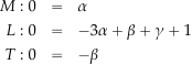
Therefore, in this case , , and , i.e.,
![\[ \Pi_{3} = (\varrho_{\infty})^{\alpha} (V_{\infty})^{\beta} (l)^{\gamma} \, h = \varrho_{\infty}^{0} V_{\infty}^{0} l^{-1} \, h = \frac{h}{l} \]](https://eaglepubs.erau.edu/app/uploads/quicklatex/quicklatex.com-de8831be0c0300b171745e7f4e692a49_l3.svg "Rendered by QuickLaTeX.com")
so
![\[ \Pi_{3} = \frac{h}{l} \]](https://eaglepubs.erau.edu/app/uploads/quicklatex/quicklatex.com-2f0b1ab578d7cf46466fbf061a75f8eb_l3.svg "Rendered by QuickLaTeX.com")
or again, this grouping can be inverted (for convenience), giving
![\[ \Pi_{3} = \frac{l}{h} = A \! R \]](https://eaglepubs.erau.edu/app/uploads/quicklatex/quicklatex.com-a4c924e806c0215fcc3460261050d05f_l3.svg "Rendered by QuickLaTeX.com")
which is a length-to-height ratio or what would be called an aspect ratio  .
.
As a result of the dimensional analysis, then
![\[ \phi \left( \frac {D}{\frac{1}{2} \varrho_{\infty} V_{\infty}^{2} \, A }, \frac{\varrho_{\infty} V_{\infty} l }{\mu_{\infty}}, \frac{l}{h} \right) = 0 \]](https://eaglepubs.erau.edu/app/uploads/quicklatex/quicklatex.com-b4f32534f7f0bf5163476384a83788a4_l3.svg "Rendered by QuickLaTeX.com")
or
![\[ \phi \left( C_{D}, Re, AR\right) = 0 \]](https://eaglepubs.erau.edu/app/uploads/quicklatex/quicklatex.com-a1abf0e7ba12c58bd0044042d1d6e05e_l3.svg "Rendered by QuickLaTeX.com")
Finally, in explicit form, the drag coefficient can be written as a function of the Reynolds number based on the banner length and the aspect ratio of the banner, i.e.,
![\[ C_{D} = \phi_{0} \left( Re, AR \right) \]](https://eaglepubs.erau.edu/app/uploads/quicklatex/quicklatex.com-53b45f484a23c6f78116eca2e2159de5_l3.svg "Rendered by QuickLaTeX.com")
Note: Try this problem again using , and as the repeating variables. What happens to the groupings?
Worked Example #24
The DBF team has observed that the banner in the previous problem begins to flutter at some critical airspeed, which results in a much higher drag on the banner. The flutter speed of the banner appears to depend on the length of the banner, , and its structural characteristics, which can be expressed in terms of a natural frequency,  . By extending the steps in the previous question, use the Buckingham method to determine the dimensionless groupings that will govern the flutter speed of the banner.
The relationship between the flutter speed  and the expected dependencies can be written in a general functional form as
![\[ V_f = f \left( \varrho_{\infty}, V_{\infty}, \mu_{\infty}, l, \omega_n \right) \]](https://eaglepubs.erau.edu/app/uploads/quicklatex/quicklatex.com-42793063d894cccd2987914a81e1e1fa_l3.svg "Rendered by QuickLaTeX.com")
or in implicit form as
![\[ g \left( V_f, \varrho_{\infty}, V_{\infty}, \mu_{\infty}, l, \omega_n \right) = 0 \]](https://eaglepubs.erau.edu/app/uploads/quicklatex/quicklatex.com-43d36821b90113b92e4bd25f8891156c_l3.svg "Rendered by QuickLaTeX.com")
Hence, in this problem , , , so there will be three products.
For each variable, the dimensions are
![\begin{eqnarray*} \left[ V_f \right] & = & \rm LT^{-1} \\ \left[ \varrho_{\infty} \right] & = & \rm ML^{-3} \\ \left[ V_{\infty} \right] & = & \rm LT^{-1} \\ \left[ \mu_{\infty} \right] & = & \rm ML^{-1}T^{-1} \\ \left[ l \right] & = & \rm L \\ \left[ \omega_n \right] & = & \rm T^{-1} \end{eqnarray*}](https://eaglepubs.erau.edu/app/uploads/quicklatex/quicklatex.com-537a3b6ff95858f6b3ace99105093c90_l3.svg "Rendered by QuickLaTeX.com")
Setting up the dimensional matrix gives
![\[ \begin{array}{l|r|r|r|r|r|r} \mbox{\small Base~unit} & V_f & \varrho_{\infty} & V_{\infty} & \mu_{\infty} & l & \Omega_n \\ \hline \text{\small Mass M:} & 0 & 1 & 0 & 1 & 0 & 0 \\ \text{\small Length L:} & 1 & -3 & 1 & -1 & 1 & 0 \\ \text{\small Time T:} & -1 & 0 & -1 & -1 & 0 & -1 \end{array} \]](https://eaglepubs.erau.edu/app/uploads/quicklatex/quicklatex.com-42edf980ca5cedbfa7c70d72b5d50582_l3.svg "Rendered by QuickLaTeX.com")
Again, as in most aerodynamic problems, , , and are a good first choice for the repeating variables. Following the Buckingham method then the products are to be determined from
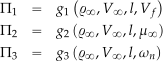
For :
![\[ \Pi_{1} = (\varrho_{\infty})^{\alpha} (V_{\infty})^{\beta} (l)^{\gamma} \, V_f \]](https://eaglepubs.erau.edu/app/uploads/quicklatex/quicklatex.com-b31524b53d650420307825a7dd6f772c_l3.svg "Rendered by QuickLaTeX.com")
In terms of the dimensions of the parameters, then
![\[ \left[ \Pi_{1} \right] = 1 = \rm M^{0}L^{0}T^{0} = \left(\rm ML^{-3} \right)^{\alpha} \left( \rm LT^{-1} \right)^{\beta} \left( \rm L \right)^{\gamma} \rm L T^{-1} \]](https://eaglepubs.erau.edu/app/uploads/quicklatex/quicklatex.com-17f852c9f31d5a1901ce06a8a84c3f3f_l3.svg "Rendered by QuickLaTeX.com")
For to be dimensionless, then
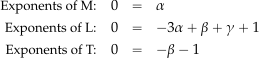
By inspection , , and  . Therefore, the first product is
![\[ \Pi_{1} = (\varrho_{\infty})^{\alpha} (V_{\infty})^{\beta} (l)^{\gamma} V_f = \varrho_{\infty}^{0} V_{\infty}^{-1} l^{0} \, V_f \]](https://eaglepubs.erau.edu/app/uploads/quicklatex/quicklatex.com-cf87142e94c401db3ef1dfdf2e9e2c70_l3.svg "Rendered by QuickLaTeX.com")
or
![\[ \Pi_{1} = \frac{V_f}{V_{\infty}} \]](https://eaglepubs.erau.edu/app/uploads/quicklatex/quicklatex.com-cbcbba31f6495b9dcf175082fe53ca0b_l3.svg "Rendered by QuickLaTeX.com")
which is a speed ratio or a dimensionless flutter speed.
For :
In terms of the dimensions of the parameters, then
![\[ \left[ \Pi_{2} \right] = 1 = \rm M^{0}L^{0}T^{0} = \left( \rm ML^{-3} \right)^{\alpha} \left( \rm LT^{-1} \right)^{\beta} \left( \rm L \right)^{\gamma} \rm M L^{-1} T^{-1} \]](https://eaglepubs.erau.edu/app/uploads/quicklatex/quicklatex.com-ae0d2f9594144ff614a81cadc30b5492_l3.svg "Rendered by QuickLaTeX.com")
For to be dimensionless, then
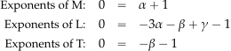
By inspection, , , and . Therefore, the second product is
![\[ \Pi_{2} = (\varrho_{\infty})^{\alpha} (V_{\infty})^{\beta} (l)^{\gamma} \mu_{\infty} = \varrho_{\infty}^{-1} V_{\infty}^{-1} l^{-1} \, \mu_{\infty} \]](https://eaglepubs.erau.edu/app/uploads/quicklatex/quicklatex.com-6aaf2c935bf2d89be1876dfde43af1b8_l3.svg "Rendered by QuickLaTeX.com")
So
![\[ \Pi_{2} = \frac{\mu_{\infty} }{\varrho_{\infty} V_{\infty} l } \]](https://eaglepubs.erau.edu/app/uploads/quicklatex/quicklatex.com-91fc270184e1bee1c78cf3a56367a5bf_l3.svg "Rendered by QuickLaTeX.com")
or
![\[ \Pi_{2} = \frac{\varrho_{\infty} V_{\infty} l }{\mu_{\infty} } \]](https://eaglepubs.erau.edu/app/uploads/quicklatex/quicklatex.com-7d3c8c6bd4e2ed1d04e1a92c92f79a67_l3.svg "Rendered by QuickLaTeX.com")
and, once again, a Reynolds number comes into the problem.
For :
![\[ \Pi_{3} = (\varrho_{\infty})^{\alpha} (V_{\infty})^{\beta} (l)^{\gamma} \, \omega_n \]](https://eaglepubs.erau.edu/app/uploads/quicklatex/quicklatex.com-772d3f8bcabb2cae77428c2051001b79_l3.svg "Rendered by QuickLaTeX.com")
In terms of the dimensions of the parameters, then
![\[ \left[ \Pi_{3} \right] = 1 = \rm M^{0}L^{0}T^{0} = \left( \rm ML^{-3} \right)^{\alpha} \left( \rm LT^{-1} \right)^{\beta} \left(\rm L \right)^{\gamma}\rm T^{-1} \]](https://eaglepubs.erau.edu/app/uploads/quicklatex/quicklatex.com-d079bfde698bd1c5d0476a3aa238fb0a_l3.svg "Rendered by QuickLaTeX.com")
For to be dimensionless, then
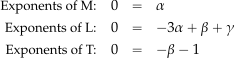
By inspection , , and . Therefore, the third product is
![\[ \Pi_{3} = (\varrho_{\infty})^{\alpha} (V_{\infty})^{\beta} (l)^{\gamma} \omega_n = \varrho_{\infty}^{0} V_{\infty}^{-1} l^{1} \ \omega_n \]](https://eaglepubs.erau.edu/app/uploads/quicklatex/quicklatex.com-8aa93a7bf2af33143f142de39d44554c_l3.svg "Rendered by QuickLaTeX.com")
or
![\[ \Pi_{3} = \frac{ \omega_n \, l }{V_{\infty} } \]](https://eaglepubs.erau.edu/app/uploads/quicklatex/quicklatex.com-52d09f4d55240b0403c91cf0e950a4fb_l3.svg "Rendered by QuickLaTeX.com")
which is a form of structural dimensionless frequency or a structural reduced frequency.
As a result of the dimensional analysis, then
![\[ \phi \left( \frac{V_f}{V_{\infty}}, \frac{\varrho_{\infty} V_{\infty} l }{\mu_{\infty} }, \frac{ \omega_n \, l }{V_{\infty} } \right) = 0 \]](https://eaglepubs.erau.edu/app/uploads/quicklatex/quicklatex.com-5da42a32b7becd6bba723b9157714d76_l3.svg "Rendered by QuickLaTeX.com")
or
or in explicit form
![\[ \frac{V_f}{V_{\infty}} = \phi_{0} \left( \frac{\varrho_{\infty} V_{\infty} l }{\mu_{\infty} }, \frac{ \omega_n \, l }{V_{\infty} } \right) \]](https://eaglepubs.erau.edu/app/uploads/quicklatex/quicklatex.com-764bf473223d607aefe5e7e7105d94f5_l3.svg "Rendered by QuickLaTeX.com")
Therefore, the dimensional analysis tells us that the dimensionless flutter speed of the banner will depend on the Reynolds number and its structural reduced frequency.
Worked Example #25
A spherical projectile of diameter is moving supersonically. The drag is assumed to depend on the freestream velocity , the freestream density , the freestream viscosity , and the freestream temperature  , as well as the heat capacities at constant volume and constant pressure,
  and
and  , respectively. Use the Buckingham method to determine the dimensionless groupings governing this problem.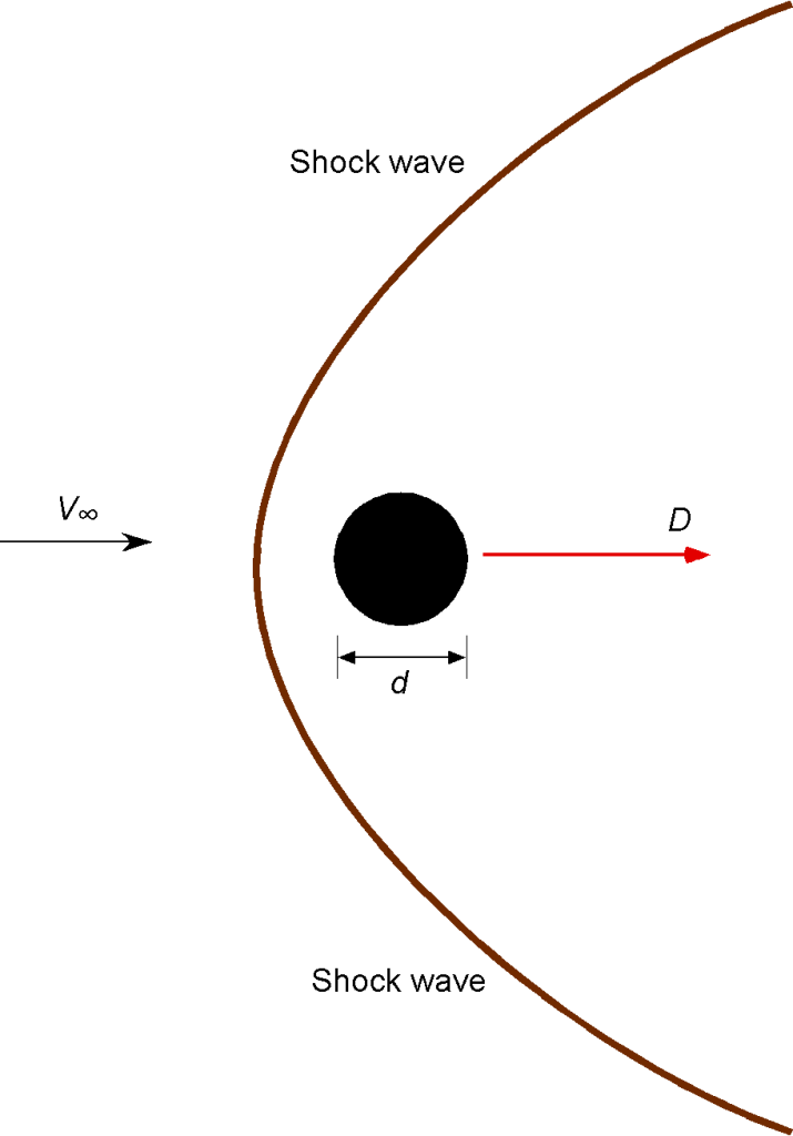
The relationship between the drag on the sphere and the given variables can be written in a general functional form as
![\[ D = f \left( \varrho_{\infty}, V_{\infty}, \mu_{\infty}, T_{\infty}, C_{\cal V}, C_p, d \right) \]](https://eaglepubs.erau.edu/app/uploads/quicklatex/quicklatex.com-ed927213a88050548c7bb097fe3188db_l3.svg "Rendered by QuickLaTeX.com")
or in implicit form as
![\[ g \left( D, \varrho_{\infty}, V_{\infty}, \mu_{\infty}, T_{\infty}, C_{\cal V}, C_p, d \right) = 0 \]](https://eaglepubs.erau.edu/app/uploads/quicklatex/quicklatex.com-0c5d88211a3b7e57fe9f70f8be8a96db_l3.svg "Rendered by QuickLaTeX.com")
Hence,  ,
,  ,
,  , and so there will be four products. Notice that temperature is explicitly defined in this case, so there are four fundamental dimensions.
For each variable, the units are
![\begin{eqnarray*} \left[ D \right] & = & \rm MLT^{-2} \\ \left[ \varrho_{\infty} \right] & = &\rm ML^{-3} \\ \left[ V_{\infty} \right] & = & \rm LT^{-1} \\ \left[ \mu_{\infty} \right] & = &\rm ML^{-1}T^{-1} \\ \left[ T_{\infty} \right] & = & \theta \\ \left[ C_{\cal V} \right] & = & \rm L^{2} T^{-2} \theta^{-1} \\ \left[ C_p \right] & = & \rm L^{2} T^{-2} \theta^{-1} \\ \left[ d \right] & = & \rm L \end{eqnarray*}](https://eaglepubs.erau.edu/app/uploads/quicklatex/quicklatex.com-83fc3189d88d965b2a58df586d5639e2_l3.svg "Rendered by QuickLaTeX.com")
The dimensional matrix is
![\[ \begin{array}{l|r|r|r|r|r|r|r|r|} \mbox{\small Base~unit} & D & \varrho_{\infty} & V_{\infty} & \mu_{\infty} & T_{\infty} & C_{\cal V} & C_p & d \\ \hline \text{\small Mass M:} & 1 & 1 & 0 & 1 & 0 & 0 & 0 & 0 \\ \text{\small Length L:} & 1 & -3 & 1 & -1 & 0 & 2 & 2 & 1 \\ \text{\small Time T:} & -2 & 0 & -1 & -1 & 0 & -2 & -2 & 0 \\ \text{\small Temperature $\theta$:} & 0 & 0 & 0 & 0 & 1 & -1 & -1 & 0 \end{array} \]](https://eaglepubs.erau.edu/app/uploads/quicklatex/quicklatex.com-a95f3574bea042e1c0eff4355f5c6a61_l3.svg "Rendered by QuickLaTeX.com")
Choose , , and as the repeating variables. They are not unique but have primary dependencies on drag and collectively include all the fundamental dimensions. Finding the determinant of the dimensional submatrix that is formed by the repeating variables shows that
![\[ \det \begin{bmatrix} 1 & 0 & 0 & 0\\ -3 & 1 & 0 & 1 \\ 0 & -1 & 0 & 0 \\ 0 & 0 & 1 & 0 \end{bmatrix} \ne 0 \]](https://eaglepubs.erau.edu/app/uploads/quicklatex/quicklatex.com-510cdc55e3ad9c67a91d13e0ac520c96_l3.svg "Rendered by QuickLaTeX.com")
so the selected repeating variables are linearly independent.
Following the Buckingham method then the products are to be determined from:
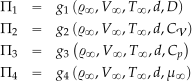
For :
![\[ \Pi_{1} = (\varrho_{\infty})^{\alpha} (V_{\infty})^{\beta} (T_{\infty})^{\gamma} (d)^{\delta} \, D \]](https://eaglepubs.erau.edu/app/uploads/quicklatex/quicklatex.com-de076e71000ff2dee622fea805cba9de_l3.svg "Rendered by QuickLaTeX.com")
In terms of the dimensions of the parameters, then
![\[ \left[ \Pi_{1} \right] = 1 = M^{0}L^{0}T^{0} \theta^{0} = \left( \rm ML^{-3} \right)^{\alpha} \left(\rm L T^{-1}\right)^{\beta} \left( \rm \theta \right)^{\gamma} \left(\rm L\right)^{\delta} \, \rm M L T^{-2} \]](https://eaglepubs.erau.edu/app/uploads/quicklatex/quicklatex.com-9ff52ae68b676973dfd14b313388c7da_l3.svg "Rendered by QuickLaTeX.com")
For to be dimensionless, then
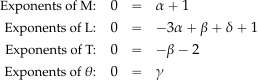
By inspection , , and  . Therefore, the first product is
![\[ \Pi_{1} = (\varrho_{\infty})^{\alpha} (V_{\infty})^{\beta} (T_{\infty})^{\gamma} (d)^{\delta} \, D = (\varrho_{\infty})^{-1} (V_{\infty})^{-2} (T_{\infty})^{0} (d)^{-2} \, D \]](https://eaglepubs.erau.edu/app/uploads/quicklatex/quicklatex.com-0df0517c5d0be1f971647f619b79c379_l3.svg "Rendered by QuickLaTeX.com")
and
![\[ \Pi_{1} = \frac{D}{\varrho_{\infty} V_{\infty}^2 \, d^2} \]](https://eaglepubs.erau.edu/app/uploads/quicklatex/quicklatex.com-26d27cf4e35ddc37884fc7e528fa7590_l3.svg "Rendered by QuickLaTeX.com")
which is a drag coefficient, which can be expressed in the conventional way as
![\[ \Pi_{1} = \frac{D}{\frac{1}{2} \varrho_{\infty} V_{\infty}^2 \, d^2} = C_D \]](https://eaglepubs.erau.edu/app/uploads/quicklatex/quicklatex.com-72bda76ba67ef6d77067fa27e8c71267_l3.svg "Rendered by QuickLaTeX.com")
For :
![\[ \Pi_{2} = (\varrho_{\infty})^{\alpha} (V_{\infty})^{\beta} (T_{\infty})^{\gamma} (d)^{\delta} \, C_{\cal V} \]](https://eaglepubs.erau.edu/app/uploads/quicklatex/quicklatex.com-793480cf31fe642a4ab6fff75b419b2a_l3.svg "Rendered by QuickLaTeX.com")
In terms of the dimensions of the parameters, then
![\[ \left[ \Pi_{2} \right] = 1 = \rm M^{0}L^{0}T^{0} \theta^{0} = \left( \rm ML^{-3} \right)^{\alpha} \left( \rm L T^{-1}\right)^{\beta} \left(\rm \theta \right)^{\gamma} \left(\rm L\right)^{\delta} \ \rm L^{2} T^{-2} \theta^{-1} \]](https://eaglepubs.erau.edu/app/uploads/quicklatex/quicklatex.com-63b5a6c335e0c064bab4f95733cf6663_l3.svg "Rendered by QuickLaTeX.com")
For to be dimensionless, then
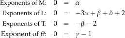
By inspection , , and  . Therefore, the second product is
![\[ \Pi_{2} = (\varrho_{\infty})^{\alpha} (V_{\infty})^{\beta} (T_{\infty})^{\gamma} (d)^{\delta} \, C_{\cal V} = (\varrho_{\infty})^{0} (V_{\infty})^{-2} (T_{\infty})^{1} (d)^{0} \, C_{\cal V} \]](https://eaglepubs.erau.edu/app/uploads/quicklatex/quicklatex.com-010f5d7b43e5768fe9775e56546e2c05_l3.svg "Rendered by QuickLaTeX.com")
and
![\[ \Pi_{2} = \frac{C_{\cal V} \, T_{\infty} }{V_{\infty}^2 } \]](https://eaglepubs.erau.edu/app/uploads/quicklatex/quicklatex.com-d4c4f36aa335615e9784eb42b92ea66a_l3.svg "Rendered by QuickLaTeX.com")
More conventionally, this ratio is written as
![\[ \Pi_{2} = \frac{V_{\infty}^2 }{C_{\cal V} \, T_{\infty} } \]](https://eaglepubs.erau.edu/app/uploads/quicklatex/quicklatex.com-d5692e0f6168bb6669189a3a2373b3d1_l3.svg "Rendered by QuickLaTeX.com")
Notice that  is the internal energy per unit mass of the freestream flow, so this dimensionless grouping represents a ratio of kinetic energy to internal energy.
For the process will be identical to that for , which is redundant. But both and have the same units, so that
![\[ \Pi_{3} = \frac{C_p}{C_{\cal V}} \]](https://eaglepubs.erau.edu/app/uploads/quicklatex/quicklatex.com-6650e9aae653de01bd4e48233dbb3726_l3.svg "Rendered by QuickLaTeX.com")
which is the familiar ratio of specific heats. This ratio would have been a product of the dimensional analysis if or had been used as a repeating variable.
For  :
:
![\[ \Pi_{4} = (\varrho_{\infty})^{\alpha} (V_{\infty})^{\beta} (T_{\infty})^{\gamma} (d)^{\delta} \ \mu_{\infty} \]](https://eaglepubs.erau.edu/app/uploads/quicklatex/quicklatex.com-2437cb8a3382dd3414de40eebb71d161_l3.svg "Rendered by QuickLaTeX.com")
In terms of the dimensions of the parameters, then
![\[ \left[ \Pi_{2} \right] = 1 =\rm M^{0}L^{0}T^{0} \theta^{0} = \rm \left( ML^{-3} \right)^{\alpha} \left( L T^{-1}\right)^{\beta} \left( \theta \right)^{\gamma} \left(L\right)^{\delta} \ \rm M L^{-1} T^{-1} \]](https://eaglepubs.erau.edu/app/uploads/quicklatex/quicklatex.com-4809868c42de38be37227f993d065ccf_l3.svg "Rendered by QuickLaTeX.com")
For to be dimensionless, then
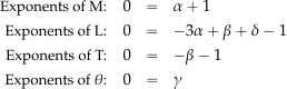
By inspection ,  , and
, and  . Therefore, the fourth product is
![\[ \Pi_{4}= (\varrho_{\infty})^{\alpha} (V_{\infty})^{\beta} (T_{\infty})^{\gamma} (d)^{\delta} \, \mu_{\infty} = (\varrho_{\infty})^{-1} (V_{\infty})^{-1} (T_{\infty})^{0} (d)^{1} \ \mu_{\infty} \]](https://eaglepubs.erau.edu/app/uploads/quicklatex/quicklatex.com-15b4666ea1108e87d79b3d9fa2949b81_l3.svg "Rendered by QuickLaTeX.com")
and
![\[ \Pi_{4} = \frac{\mu_{\infty}}{\varrho_{\infty} V_{\infty} d} \]](https://eaglepubs.erau.edu/app/uploads/quicklatex/quicklatex.com-82eff491c664210b53ae6a8e33ae853e_l3.svg "Rendered by QuickLaTeX.com")
or just
![\[ \Pi_{4} = \frac{\varrho_{\infty} V_{\infty} d}{\mu_{\infty}} \]](https://eaglepubs.erau.edu/app/uploads/quicklatex/quicklatex.com-3f4dd240bbc040df336e24435cd0be5a_l3.svg "Rendered by QuickLaTeX.com")
which is the Reynolds number.
As a result of the dimensional analysis, then
![\[ \phi \left( \frac{D}{\frac{1}{2} \varrho_{\infty} V_{\infty}^2 \, d^2}, \, \frac{V_{\infty}^2 }{C_{\cal V} \, \, T_{\infty} }, \, \frac{C_p}{C_{\cal V}}, \, \frac{\varrho_{\infty} V_{\infty} d}{\mu_{\infty}} \right) = 0 \]](https://eaglepubs.erau.edu/app/uploads/quicklatex/quicklatex.com-7b9aeaa24539a659a498da4fedcea49e_l3.svg "Rendered by QuickLaTeX.com")
or in explicit form
![\[ \frac{D}{\frac{1}{2} \varrho_{\infty} V_{\infty}^2 \, d^2} = \phi_0 \left( \frac{V_{\infty}^2 }{C_{\cal V} \, T_{\infty} }, \, \frac{C_p}{C_{\cal V}}, \, \frac{\varrho_{\infty} V_{\infty} d}{\mu_{\infty}} \right) \]](https://eaglepubs.erau.edu/app/uploads/quicklatex/quicklatex.com-fc0098faed93e19400a799f83cc71dd5_l3.svg "Rendered by QuickLaTeX.com")
But the critical grouping that comes out of this problem is
Worked Example #26
A force is applied at the tip of a cantilevered wing of length and the second moment of area . The modulus of elasticity of the material used for the wing is . When the force is applied, the tip deflection is  . Use the Buckingham method to find the dimensionless groupings governing this problem.
The relationship between the force and the tip deflection can be written in the general functional form as
![\[ z_d = f \left( F, L_w, I, E \right) \]](https://eaglepubs.erau.edu/app/uploads/quicklatex/quicklatex.com-022dec43a14badb6425aa76245e80924_l3.svg "Rendered by QuickLaTeX.com")
or in implicit form as
![\[ g \left(z_d, F, L_w, I, E \right) = 0 \]](https://eaglepubs.erau.edu/app/uploads/quicklatex/quicklatex.com-a8bb259b0d0e05373352d8fea0984d33_l3.svg "Rendered by QuickLaTeX.com")
where  denotes the length of the wing to avoid confusion with the length dimension. Hence, , ,
  , and so there will be two products.
For each variable, the units are
![\begin{eqnarray*} \left[ z_d \right] & = & \rm L \\ \left[ F \right] & = & \rm M L T^{-2} \\ \left[ L_w \right] & = & \rm L \\ \left[ I \right] & = & \rm L^4 \\ \left[ E \right] & = & \rm M L^{-1} T^{-2} \end{eqnarray*}](https://eaglepubs.erau.edu/app/uploads/quicklatex/quicklatex.com-6fbcde40f55b01d707810e4215d99571_l3.svg "Rendered by QuickLaTeX.com")
The dimensional matrix is
![\[ \begin{array}{l|r|r|r|r|r} \mbox{\small Base~unit} & z_d & F & L_w & I & E \\ \hline \text{\small Mass M:} & 0 & 1 & 0 & 0 & 1 \\ \text{\small Length L:} & 1 & 1 & 1 & 4 & -1 \\ \text{\small Time T:} & 0 & -2 & 0 & 0 & -2 \end{array} \]](https://eaglepubs.erau.edu/app/uploads/quicklatex/quicklatex.com-d129f13c99bc17927673ab79fa4906fd_l3.svg "Rendered by QuickLaTeX.com")
This problem poses a dilemma because the choice of the repeating variables here is not apparent. Suppose , , and are selected as the repeating variables. In that case, they will not be linearly independent. If , , and are chosen as the repeating variables (try it!), then the solution to the problem becomes indeterminate, i.e., the dimensionless groupings cannot be uniquely solved for.
The accepted solution to this dilemma is to reduce the number of repeating variables by one and create a third grouping. If and are chosen as repeating variables, which are linearly independent and include all of the fundamental dimensions, then, following the Buckingham method, the three products will be
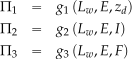
For , then
![\[ \Pi_{1} = (L_w)^{\alpha} (E^{\beta}) \, z_d \]](https://eaglepubs.erau.edu/app/uploads/quicklatex/quicklatex.com-a7f8156139c77294382bb26dad813397_l3.svg "Rendered by QuickLaTeX.com")
In terms of the dimensions of the parameters, then
![\[ \left[ \Pi_{1} \right] = 1 = \rm M^{0}L^{0}T^{0} = \rm \left( L \right)^{\alpha} \left( M L^{-1} T^{-2} \right)^{\beta} L \]](https://eaglepubs.erau.edu/app/uploads/quicklatex/quicklatex.com-cf583faec2c87de2d048aec283c2086f_l3.svg "Rendered by QuickLaTeX.com")
For to be dimensionless, then
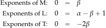
By inspection and , so the first product is
![\[ \Pi_{1} = (L_w)^{\alpha} (E^{\beta}) \, z_d = (L_w)^{-1} (E^0) \, z_d \]](https://eaglepubs.erau.edu/app/uploads/quicklatex/quicklatex.com-3419952ca9ab8352f334d9062a4f3902_l3.svg "Rendered by QuickLaTeX.com")
so
![\[ \Pi_{1} = \frac{ z_d}{L_w} \]](https://eaglepubs.erau.edu/app/uploads/quicklatex/quicklatex.com-b61d4a69a13ce57619f5339045cfb9ac_l3.svg "Rendered by QuickLaTeX.com")
i.e., a dimensionless displacement is an expected, if not obvious, grouping.
For , then
![\[ \Pi_{2} = (L_w)^{\alpha} (E^{\beta}) \, I \]](https://eaglepubs.erau.edu/app/uploads/quicklatex/quicklatex.com-29dc155a6a0be28c9448aba5f16fd894_l3.svg "Rendered by QuickLaTeX.com")
In terms of the dimensions of the parameters, then
![\[ \left[ \Pi_{2} \right] = 1 = \rm M^{0}L^{0}T^{0} = \rm \left( L \right)^{\alpha} \left( M L^{-1} T^{-2} \right)^{\beta} L^4 \]](https://eaglepubs.erau.edu/app/uploads/quicklatex/quicklatex.com-79477e27464568b72899c97a09b43ccb_l3.svg "Rendered by QuickLaTeX.com")
For to be dimensionless, then
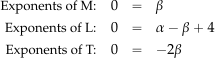
By inspection  and , so the second product is
![\[ \Pi_{2} = (L_w)^{\alpha} (E^{\beta}) \, I = (L_w)^{-4} (E^0) \, I \]](https://eaglepubs.erau.edu/app/uploads/quicklatex/quicklatex.com-0b67af0649305c775e27963799a0714b_l3.svg "Rendered by QuickLaTeX.com")
and so
![\[ \Pi_{2} = \frac{ I}{L_w^4} \]](https://eaglepubs.erau.edu/app/uploads/quicklatex/quicklatex.com-3dfac234772fa53a460fd609b804954c_l3.svg "Rendered by QuickLaTeX.com")
which is a dimensionless form of the second moment of area.
For , then
![\[ \Pi_{3} = (L_w)^{\alpha} (E^{\beta}) \, F \]](https://eaglepubs.erau.edu/app/uploads/quicklatex/quicklatex.com-7308e37da72ca018f158225b678aa2f6_l3.svg "Rendered by QuickLaTeX.com")
In terms of the dimensions of the parameters, then
![\[ \left[ \Pi_{3} \right] = 1 =\rm M^{0}L^{0}T^{0} = \rm \left( L \right)^{\alpha} \left( M L^{-1} T^{-2} \right)^{\beta} M L T^{-2} \]](https://eaglepubs.erau.edu/app/uploads/quicklatex/quicklatex.com-a99f7920657fa05ef7597a9381eae255_l3.svg "Rendered by QuickLaTeX.com")
For to be dimensionless, then
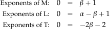
By inspection and , so the third product is
![\[ \Pi_{3} = (L_w)^{\alpha} (E^{\beta}) \, I = (L_w)^{-2} (E^{-1}) \, F \]](https://eaglepubs.erau.edu/app/uploads/quicklatex/quicklatex.com-a330fb58d68e601a2bf360bfb9e2555b_l3.svg "Rendered by QuickLaTeX.com")
so
![\[ \Pi_{3} = \frac{ F}{E \, L_w^2} \]](https://eaglepubs.erau.edu/app/uploads/quicklatex/quicklatex.com-a850da4c7f342eb1edfdc83ba98909d2_l3.svg "Rendered by QuickLaTeX.com")
which is a form of dimensionless force or force coefficient.
Finally, all three groupings have been determined, so the final result in functional form is
![\[ \phi \left( \frac{ z_d}{L_w}, \frac{ I}{L_w^4}, \frac{ F}{E \, L_w^2} \right) = 0 \]](https://eaglepubs.erau.edu/app/uploads/quicklatex/quicklatex.com-0d5f9641d1ecda19b8e01806d7391311_l3.svg "Rendered by QuickLaTeX.com")
or
![\[ \frac{z_d}{L_w} = \phi_0 \left( \frac{ I}{L_w^4}, \frac{ F}{E \, L_w^2} \right) \]](https://eaglepubs.erau.edu/app/uploads/quicklatex/quicklatex.com-de1485813948bc4eb8d6ea48a4d0994c_l3.svg "Rendered by QuickLaTeX.com")
Worked Example #27
The ERAU wind tunnel uses tiny oil-based aerosol particles of characteristic size,  , and density,
  , to make flow measurements using a method called Particle Image Velocimetry (PIV). The characteristic time required for the aerosol particle to adjust to a sudden change in flow speed is called the particle relaxation time
  , which is given by the equation
![\[ \tau_p = \frac{\varrho_p D_p^2}{18 \mu_{\infty}} \]](https://eaglepubs.erau.edu/app/uploads/quicklatex/quicklatex.com-4427e9374a1b6e3f39aaddf00b95792e_l3.svg "Rendered by QuickLaTeX.com")
where is the viscosity of the flow. First, verify that the primary units of have dimensions of time. Second, find a dimensionless form for the time constant based on a characteristic flow velocity, , and a characteristic length, . Comment on your result. Do you see anything interesting?
The information given is
and the dimensions of are time. For each variable, the units are
![\begin{eqnarray*} \left[ \varrho_p \right] & = & \rm M L^{-3} \\ \left[ D_p \right] & = & \rm L \\ \left[ \mu_{\infty} \right] & = & \rm M L^{-1} T^{-1} \\ \end{eqnarray*}](https://eaglepubs.erau.edu/app/uploads/quicklatex/quicklatex.com-aaf2070e5feb0eba2dacf33378a0896d_l3.svg "Rendered by QuickLaTeX.com")
so
![\[ \left[ \tau_p \right] = \frac{\rm (M L^{-3} ) (L^2)}{\rm M L^{-1} T^{-1}} = \frac{ \rm M L^{-1}}{\rm M L^{-1} T^{-1}} = \rm T \]](https://eaglepubs.erau.edu/app/uploads/quicklatex/quicklatex.com-b285de0becfc4c0ea2ab91ff21ddc9ff_l3.svg "Rendered by QuickLaTeX.com")
which confirms that the dimensions of are time.
A dimensionless form of is required based on a characteristic flow velocity, , and a characteristic length, . The ratio  has dimensions of time, so that a dimensionless form could be
![\[ \hat{\tau}_p = \frac{\varrho_p D_p^2}{18 \mu_{\infty}}\ \frac{V}{L} = \frac{\varrho_p V D_p}{18 \mu_{\infty}} \, \frac{D_p}{L} = \frac{1}{18} \left( \frac{\varrho_p V D_p}{ \mu_{\infty}} \right) \left( \frac{D_p}{L} \right) \]](https://eaglepubs.erau.edu/app/uploads/quicklatex/quicklatex.com-e27137ba09ff519b1bde9e4e9cc36e03_l3.svg "Rendered by QuickLaTeX.com")
This outcome is interesting because it involves a Reynolds number based on particle diameter and the particle diameter ratio to the length scale. Therefore, the higher the Reynolds number and/or the bigger the particle, the longer it will take to adjust to any changes in the flow conditions.
Worked Example #28
Based on experiments performed with a wind turbine, it is determined that its power output is a function of the size of the wind turbine as characterized by its radius , the rotational angular velocity of the turbine , the wind speed , and the air density . Using the Buckingham method, determine the dimensionless groupings describing this problem.
For this problem, the power output can be written as
![\[ P = f \left( R, \Omega, V_{\infty}, \varrho_{\infty} \right) \]](https://eaglepubs.erau.edu/app/uploads/quicklatex/quicklatex.com-552968fe20ca0be2dd7ad3c79498ed56_l3.svg "Rendered by QuickLaTeX.com")
In implicit form, then
![\[ \phi_1 \left( R, \Omega, V_{\infty}, \varrho_{\infty}, P \right) = 0 \]](https://eaglepubs.erau.edu/app/uploads/quicklatex/quicklatex.com-fa224ea29fda9dd00ffd3d23c5c3d6b2_l3.svg "Rendered by QuickLaTeX.com")
Therefore, and again  so there will be two products.
The dimensional matrix is
![\[ \begin{array}{l|r|r|r|r|r} \mbox{\small Base~unit} & R & \Omega & V_{\infty} & \varrho_{\infty} & P \\ \hline \text{\small Mass M:} & 0 & 0 & 0 & 1 & 1 \\ \text{\small Length L:} & 1 & 0 & 1 & -3 & 2 \\ \text{\small Time T:} & 0 & -1 & -1 & 0 & -3 \end{array} \]](https://eaglepubs.erau.edu/app/uploads/quicklatex/quicklatex.com-1e3c44882435820bc781337ea070d3e3_l3.svg "Rendered by QuickLaTeX.com")
Notice the base dimensions of power are M L T.
Now, the repeating variable must be chosen. In this case, a good choice is , , and , which will primarily influence power production from the turbine. They also collectively include all of the fundamental dimensions of mass, length, and time, and they are linearly independent just by inspection.
For the first product then
![\[ \Pi_{1} = \phi_2 \left(R, V_{\infty}, \varrho_{\infty}, P \right) \]](https://eaglepubs.erau.edu/app/uploads/quicklatex/quicklatex.com-c022155f4ed8aeb91dcf54c6d75d9d09_l3.svg "Rendered by QuickLaTeX.com")
and for the second product then
![\[ \Pi_{2} = \phi_3 \left(R, V_{\infty}, \varrho_{\infty}, \Omega \right) \]](https://eaglepubs.erau.edu/app/uploads/quicklatex/quicklatex.com-cd53e048e261313e3f1e4585222d7d46_l3.svg "Rendered by QuickLaTeX.com")
Continuing with the first product then
![\[ \Pi_{1} = (R)^{\alpha} (V_{\infty})^{\beta} (\varrho_{\infty})^{\gamma} P \]](https://eaglepubs.erau.edu/app/uploads/quicklatex/quicklatex.com-fb0093eed096238b64e7d95533a37035_l3.svg "Rendered by QuickLaTeX.com")
and terms of the dimensions, then
![\[ \left[ \Pi_{1} \right] = \rm M^{0}L^{0}T^{0} = \rm (L)^{\alpha} (L T^{-1} )^{\beta} (M L^{-3} )^{\gamma} M L^{2} T^{-3} \]](https://eaglepubs.erau.edu/app/uploads/quicklatex/quicklatex.com-a4c8839ca497150645c1ae01447081e1_l3.svg "Rendered by QuickLaTeX.com")
For to be dimensionless, then
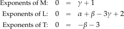
Therefore, = -3, = -1, and , so the product is
![\[ \Pi_1 = (R)^{-2} (V_{\infty})^{-3} (\varrho_{\infty})^{-1} P \]](https://eaglepubs.erau.edu/app/uploads/quicklatex/quicklatex.com-9f8bf0ed101a5d03a9255ff522662a29_l3.svg "Rendered by QuickLaTeX.com")
or
![\[ \Pi_1 = \frac{P}{\varrho_{\infty} R^2 V_{\infty}^{3}} \]](https://eaglepubs.erau.edu/app/uploads/quicklatex/quicklatex.com-e51437f777bda1e24502b734dabd1ab0_l3.svg "Rendered by QuickLaTeX.com")
which is a form of power coefficient, i.e.,
![\[ C_P = \frac{P}{\varrho_{\infty} R^2 V_{\infty}^{3}} \]](https://eaglepubs.erau.edu/app/uploads/quicklatex/quicklatex.com-3afb4578fd16e5c62c330aabe480184c_l3.svg "Rendered by QuickLaTeX.com")
Considering now the second product then
![\[ \Pi_{2} = (R)^{\alpha} (V_{\infty})^{\beta} (\varrho_{\infty})^{\gamma} \Omega \]](https://eaglepubs.erau.edu/app/uploads/quicklatex/quicklatex.com-d65fbaaf4ec8ceb601726d575706ef5c_l3.svg "Rendered by QuickLaTeX.com")
and terms of the dimensions, then
![\[ \left[ \Pi_{2} \right] = \rm M^{0}L^{0}T^{0} = \rm (L)^{\alpha} (L T^{-1} )^{\beta} (M L^{-3} )^{\gamma} T^{-1} \]](https://eaglepubs.erau.edu/app/uploads/quicklatex/quicklatex.com-af0a5189fe7b1fd2ddbad34caecdae84_l3.svg "Rendered by QuickLaTeX.com")
For to be dimensionless, then
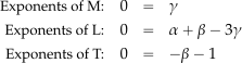
Therefore, = -1, = 0, and , so the product is
![\[ \Pi_2 = (R)^{1} (V_{\infty})^{-1} (\varrho_{\infty})^{0} \Omega \]](https://eaglepubs.erau.edu/app/uploads/quicklatex/quicklatex.com-df7cedd6f02dfdd6b70cfaaecd117fa3_l3.svg "Rendered by QuickLaTeX.com")
or
![\[ \Pi_2 = \frac{\Omega R} {V_{\infty}} \quad \mbox{or} \quad \frac{V_{\infty}}{\Omega R} \]](https://eaglepubs.erau.edu/app/uploads/quicklatex/quicklatex.com-08ff45d600e9be3549b8826c7c024064_l3.svg "Rendered by QuickLaTeX.com")
which is a form of an advance ratio or tip speed ratio, i.e.,
![\[ J = \frac{V_{\infty}}{\Omega R} \]](https://eaglepubs.erau.edu/app/uploads/quicklatex/quicklatex.com-3aadecfcae8b0235619d132ac2332156_l3.svg "Rendered by QuickLaTeX.com")
Therefore, based on the information given, the power output of the wind turbine in terms of a power coefficient  is related to the wind speed in the form of a tip speed ratio
  , i.e.,
![\[ \frac{P}{\varrho_{\infty} R^2 V_{\infty}^{3}} = \phi \left( \frac{V_{\infty}}{\Omega R} \right) \]](https://eaglepubs.erau.edu/app/uploads/quicklatex/quicklatex.com-6b342f57885c39c9399d72c9ced12af8_l3.svg "Rendered by QuickLaTeX.com")
or
![\[ C_P = \phi (J) \]](https://eaglepubs.erau.edu/app/uploads/quicklatex/quicklatex.com-71524c9a73cebea49660f852b42545a3_l3.svg "Rendered by QuickLaTeX.com")
Worked Example #29
A sphere is located in a pipe through which a liquid flows. The drag force  on the sphere is assumed to be a function of the sphere’s diameter , the pipe diameter , the average flow velocity , and the fluid density .
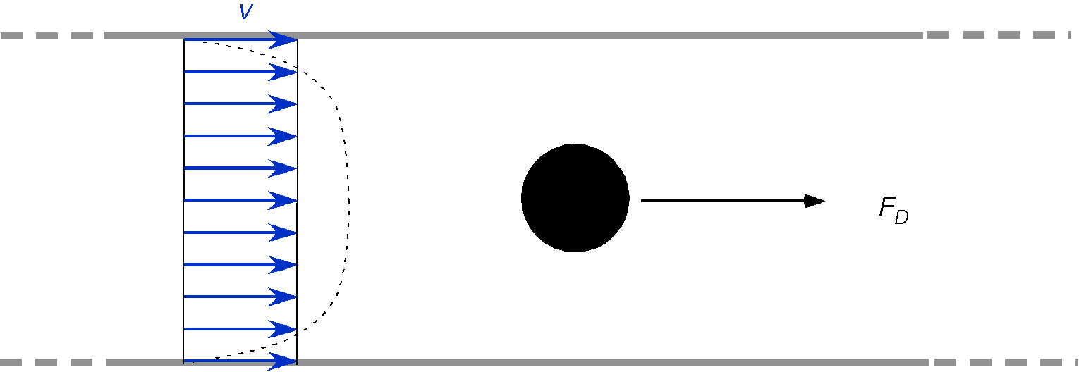 1. Write down the functional expression for the drag force in terms of the parameters given above.
2. Write down the dimensional matrix for this problem in terms of base dimensions M, L, and T.
3. Determine the relevant groups for this problem.
4. If the drag force on the sphere with = 0.1 m and = 0.07 m in a specific liquid flowing at an average flow speed of 3 m/s is 600 N, what would the drag force be on a sphere with = 0.4 m and = 0.28 m at 6.7 m/s using the same liquid? Assume that = 900 kg m.
1. In explicit form, then
![\[ F_D = \phi \left( d, D, V, \varrho \right) \]](https://eaglepubs.erau.edu/app/uploads/quicklatex/quicklatex.com-a442e0b810b6b0340770116f18a21738_l3.svg "Rendered by QuickLaTeX.com")
or in the implicit form, then
![\[ \phi_1 \left( F_D, d, D, V, \varrho \right) = 0 \]](https://eaglepubs.erau.edu/app/uploads/quicklatex/quicklatex.com-a2771568fc14c08f48dbcd026d21177f_l3.svg "Rendered by QuickLaTeX.com")
2. Setting up the dimensional matrix for this problem gives
![\[ \begin{array}{l|r|r|r|r|r|r|} \mbox{\small Base~unit} & F_D & d & D & V & \varrho \\ \hline \text{\small Mass M:} & 1 & 0 & 0 & 0 & 1 \\ \text{\small Length L:} & 1 & 1 & 1 & 1 & -3 \\ \text{\small Time T:} & -2 & 0 & 0 & -1 & 0 \\ \end{array} \]](https://eaglepubs.erau.edu/app/uploads/quicklatex/quicklatex.com-0776cdb47f4a6ae8075a823fae7036ec_l3.svg "Rendered by QuickLaTeX.com")
3. In this case, (five variables), and by inspection, all of , , and are involved, so (i.e., three fundamental dimensions) and there are two products to determine.
4. Use , , and as the repeating variables. This choice includes all the fundamental dimensions, and it is obvious that they are all linearly independent. Following the Buckingham method then the two products are
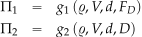
So the first product is
![\[ \Pi_{1} = (\varrho)^{\alpha} (V)^{\beta} d^{\gamma} \, F_D \]](https://eaglepubs.erau.edu/app/uploads/quicklatex/quicklatex.com-a9df7ad7933e18560c2b3d366dbab483_l3.svg "Rendered by QuickLaTeX.com")
and terms of the dimensions, then
![\[ \left[ \Pi_{1} \right] = \rm M^{0}L^{0}T^{0} = \rm (ML^{-3})^{\alpha} (L T^{-1} )^{\beta} (L)^{\gamma} \, M L T^{-2} \]](https://eaglepubs.erau.edu/app/uploads/quicklatex/quicklatex.com-f64390c3712d132e0f037c56d26fbe73_l3.svg "Rendered by QuickLaTeX.com")
For to be dimensionless then
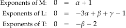
Therefore, , , and so the product is
![\[ \Pi_1 = (\varrho)^{-1} (V)^{-2} d^{-2} F_D = \frac{F_d}{\varrho \, V^2 d^2} = C_{F} \]](https://eaglepubs.erau.edu/app/uploads/quicklatex/quicklatex.com-f583f72ac6128035675e33b317739d3d_l3.svg "Rendered by QuickLaTeX.com")
which is a force coefficient.
For the second product then
![\[ \Pi_{2} = (\varrho)^{\alpha} (V)^{\beta} (d^{\gamma}) D \]](https://eaglepubs.erau.edu/app/uploads/quicklatex/quicklatex.com-6a2f281025f06d45343a45d698631d7c_l3.svg "Rendered by QuickLaTeX.com")
and terms of the dimensions, then
![\[ \left[ \Pi_{2} \right] = \rm M^{0}L^{0}T^{0} =\rm (ML^{-3})^{\alpha} (L T^{-1} )^{\beta} (L)^{\gamma} \, L \]](https://eaglepubs.erau.edu/app/uploads/quicklatex/quicklatex.com-76742958a93a92a176aeddb056b3dd51_l3.svg "Rendered by QuickLaTeX.com")
For to be dimensionless, then
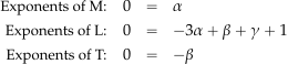
Therefore, = 0 and = 0, and = -1 so the product is
![\[ \Pi_2 = (\varrho)^{0} (V)^{0} (d^{-1}) D = \frac{D}{d} \]](https://eaglepubs.erau.edu/app/uploads/quicklatex/quicklatex.com-089526e37d3b603dc77b524cc75a707c_l3.svg "Rendered by QuickLaTeX.com")
which is a dimensionless length. Therefore,
![\[ \phi_2 \left( \Pi_1, \Pi_2\right) = 0 \]](https://eaglepubs.erau.edu/app/uploads/quicklatex/quicklatex.com-a5bd5cb10d153fb06e962fa283a9884f_l3.svg "Rendered by QuickLaTeX.com")
and so finally, in explicit form, then
![\[ C_F = \phi_3 \left( \frac{D}{d} \right) \]](https://eaglepubs.erau.edu/app/uploads/quicklatex/quicklatex.com-3680098c71e5bdb9b2d8ee7d4709ecc6_l3.svg "Rendered by QuickLaTeX.com")
5. To examine dimensional similitude, for both cases, the force coefficients must be the same so
![\[ C_F = \frac{F_{D_{1}}}{\varrho V_1^2 d_1^2} = \frac{F_{D_{2}}}{\varrho V_2^2 d_2^2} \]](https://eaglepubs.erau.edu/app/uploads/quicklatex/quicklatex.com-aa4fffde91ca4ef66fe58aa43b5d609f_l3.svg "Rendered by QuickLaTeX.com")
so by rearrangement, then
![\[ F_{D_{2}} = F_{D_{1}} \left( \frac{V_2^2}{V_1^2} \right) \left( \frac{d_2^2}{d_1^2} \right) = 600 \left( \frac{6.7^2}{3.0^2} \right) \left( \frac{0.28^2}{0.07^2} \right) = 47,882.7~\mbox{N} \]](https://eaglepubs.erau.edu/app/uploads/quicklatex/quicklatex.com-44e46cdc5799d72e535a93bd519e786e_l3.svg "Rendered by QuickLaTeX.com")
Confirming geometric similarity gives
![\[ \left(\frac{D_1}{d_1} \right) \left(\frac{d_2}{D_2} \right) = \left(\frac{0.1}{0.07} \right) \left(\frac{0.28}{0.4} \right) = 1 \]](https://eaglepubs.erau.edu/app/uploads/quicklatex/quicklatex.com-283c443c3c8a1ab948619f3d9475559e_l3.svg "Rendered by QuickLaTeX.com")
Worked Example #30
The singing sounds produced by power lines in the wind are called Aeolian tones, caused by vortex shedding behind the lines. The frequency of the sound, , is a function of the diameter of the wires, , the wind speed, , the density of the air, , and its dynamic viscosity, .
1. Write down the functional relationship for the frequency in terms of the other parameters in implicit and explicit form.
2. How many base dimensions and groupings are involved in this problem
3. Write down the dimensional matrix for the problem.
4. Use the Buckingham method to determine the dimensionless parameter(s) that describes this problem.
5. Rewrite the functional relationship in terms of the dimensionless parameter(s).
1. The frequency of the sound can be written explicitly as
![\[ f = \phi_1 (d, V, \varrho, \mu) \]](https://eaglepubs.erau.edu/app/uploads/quicklatex/quicklatex.com-b94a4bc46db83b8957ee25f69c176e4a_l3.svg "Rendered by QuickLaTeX.com")
or implicitly as
![\[ \phi_2 (d, V, \varrho, \mu, f) = 0 \]](https://eaglepubs.erau.edu/app/uploads/quicklatex/quicklatex.com-b93cbd6d57bde268bf19db432246d11a_l3.svg "Rendered by QuickLaTeX.com")
2. The number of variables is five, so , and the number of base dimensions (mass, length, and time are all involved) is 3, so . This means there are so two groupings.
3. The dimensional matrix is
![\[ \begin{array}{l|r|r|r|r|r|r} \mbox{\small Base~unit} & d & V & \varrho & \mu & f \\ \hline \text{\small Mass M:} & 0 & 0 & 1 & 1 & 0 \\ \text{\small Length L:} & 1 & 1 & -3 & -1 & 0 \\ \text{\small Time T:} & 0 & -1 & 0 & -1 & -1 \end{array} \]](https://eaglepubs.erau.edu/app/uploads/quicklatex/quicklatex.com-63e1cc2971e46f7038d61b4ad6b3258f_l3.svg "Rendered by QuickLaTeX.com")
4. Choose the variables as , , and , which are a standard choice for aerodynamic problems. It is now possible to proceed to find the two groups, i.e.,
![\[ \Pi_1 = g_1(d,V,\varrho,\mu) \]](https://eaglepubs.erau.edu/app/uploads/quicklatex/quicklatex.com-d79f0a0a2cb1510204cb7f6baafc039d_l3.svg "Rendered by QuickLaTeX.com")
and
![\[ \Pi_2 = g_2(d,V,\varrho,f) \]](https://eaglepubs.erau.edu/app/uploads/quicklatex/quicklatex.com-e83227d3fc711bb039cfdcee1230ad62_l3.svg "Rendered by QuickLaTeX.com")
For then
![\[ \Pi_1 = g_1(d, V, \varrho, \mu) \]](https://eaglepubs.erau.edu/app/uploads/quicklatex/quicklatex.com-2c000bd523cb201b870abf758f4b723a_l3.svg "Rendered by QuickLaTeX.com")
Raising the repeating variables to unknown powers gives
![\[ \left[ \Pi_1 \right] = d^{\alpha} \, V^{\beta} \, \varrho^{\gamma} \, \mu = 1 \]](https://eaglepubs.erau.edu/app/uploads/quicklatex/quicklatex.com-f819f107072e6264f00c574c8a4e1bf3_l3.svg "Rendered by QuickLaTeX.com")
In terms of dimensions, then
![\[ \rm M^0 L^0 T^0 = 1 = \rm L^{\alpha} \, (LT^{-1})^{\beta} \, (ML^{-3})^{\gamma} \, ML^{-1}T^{-1} \]](https://eaglepubs.erau.edu/app/uploads/quicklatex/quicklatex.com-c95674ec09c5163495c3c92ea7d669d5_l3.svg "Rendered by QuickLaTeX.com")
For to be dimensionless, the powers of each base dimension must add to zero, i.e.
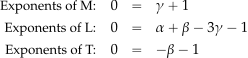
Solving the equations gives , , and so
![\[ \Pi_1 = d^{-1} \, V^{-1} \, \varrho^{-1} \, \mu = \frac{\mu} {\varrho Vd} \]](https://eaglepubs.erau.edu/app/uploads/quicklatex/quicklatex.com-0c9a10296510bb3d51acab7923cc0721_l3.svg "Rendered by QuickLaTeX.com")
which is the inverse of the Reynolds number, so the grouping can be inverted (still having a dimensionless grouping), giving
![\[ \Pi_1 = \frac {\varrho Vd} {\mu} = Re \]](https://eaglepubs.erau.edu/app/uploads/quicklatex/quicklatex.com-e4ef29816734a59601be855e683a4338_l3.svg "Rendered by QuickLaTeX.com")
Solving for gives
![\[ \Pi_2 = g_2(d, V, \varrho, f) \]](https://eaglepubs.erau.edu/app/uploads/quicklatex/quicklatex.com-2a53103a680e20f03c4afbee9200b51e_l3.svg "Rendered by QuickLaTeX.com")
so
![\[ \left[ \Pi_2 \right] = d^{\alpha} \, V^{\beta} \, \varrho^{\gamma} \, f = 1 \]](https://eaglepubs.erau.edu/app/uploads/quicklatex/quicklatex.com-0ae3f6d58deb33d2f7460aa98917dae2_l3.svg "Rendered by QuickLaTeX.com")
In terms of dimensions, then
![\[ \rm M^0 L^0 T^0 = 1 = \rm L^{\alpha} \, (LT^{-1})^{\beta} \, (ML^{-3})^{\gamma} \ T^{-1} \]](https://eaglepubs.erau.edu/app/uploads/quicklatex/quicklatex.com-f8583df444fe4290950cdd569c553cbf_l3.svg "Rendered by QuickLaTeX.com")
For to be dimensionless, the powers of each base dimension must add to zero, i.e.
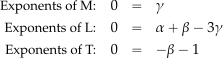
Solving the equations gives , , and so
![\[ \Pi_2 = d^{1} \, V^{-1} \, \varrho^{0} \, f = \frac{f d} {V} \]](https://eaglepubs.erau.edu/app/uploads/quicklatex/quicklatex.com-c8fe10b94f074c36fd61d5c95e81956f_l3.svg "Rendered by QuickLaTeX.com")
which is a Strouhal number, i.e.,
![\[ \Pi_2 = \frac{f d} {V} = St \]](https://eaglepubs.erau.edu/app/uploads/quicklatex/quicklatex.com-22728fa53b7bbafe317ce7af12921823_l3.svg "Rendered by QuickLaTeX.com")
5. Therefore, based on the preceding analysis, then
![\[ \phi_3(\Pi_1, \Pi_2) = 0 \]](https://eaglepubs.erau.edu/app/uploads/quicklatex/quicklatex.com-e5d5381d484229cb48504c6ab65f70dc_l3.svg "Rendered by QuickLaTeX.com")
or
![\[ \phi_3 (\frac{\varrho V d} {\mu}, \frac{f \, d} {V}) = 0 \]](https://eaglepubs.erau.edu/app/uploads/quicklatex/quicklatex.com-cffa62b42b092060bb744c25762b9464_l3.svg "Rendered by QuickLaTeX.com")
or
![\[ St = \phi_4 (Re) \]](https://eaglepubs.erau.edu/app/uploads/quicklatex/quicklatex.com-0ff827d9503705ea64f406b4c62c4447_l3.svg "Rendered by QuickLaTeX.com")
So, the Strouhal number is a function of the Reynolds number.
Worked Example #31
Using Worked Example #30 as a basis, it is desired to replicate the physics of the singing sound and study it in a low-speed wind tunnel. The actual power wires have a diameter of 2.2 cm and are known to sing at wind speeds between 25 mph and 70 mph. How would you develop a wind tunnel test plan to study this problem? The equivalent wire available for the wind tunnel test is 1.1 cm in diameter, and the wires are strung across the test section’s width. The tunnel can reach a maximum flow speed of 75 ft/s. Is it possible to obtain the dynamic similarity of this problem in the wind tunnel test? If not, why not, and what other considerations might be given to the wind tunnel test?
Based on the previous problem, the two relevant similarity parameters in t, in this case, the Reynolds number and the Strouhal number, and the Strouhal number is a function of the Reynolds number. For the actual power wires, the Reynolds number based on diameter = 2.2 cm will be
![\[ Re = \frac{\varrho \, V \, d}{\mu} = \frac{1.225 \times 70.0 \times 0.447 \times 0.022}{0.000017894} = 471,256 \]](https://eaglepubs.erau.edu/app/uploads/quicklatex/quicklatex.com-20da54be1016073cb1e5aa8379d465e2_l3.svg "Rendered by QuickLaTeX.com")
using the highest wind speed of 70 mph and MSL ISA values for air. Notice that 70 mph is equivalent to 102.67 ft/s.
The wire available in the wind tunnel is only 1.1 cm in diameter, i.e.,  . So, to get the same Reynolds number, the flow speed will need to be twice, i.e., 140 mph or 205.3 ft/s, but this is significantly less than the wind tunnel’s maximum flow speed. Even if the wire used in the tunnel were 2.2 cm in diameter, the required flow speed to match the Reynolds number would be higher than is attainable.
One solution would be to use a wire of a diameter of, say, 3.3 cm in the wind tunnel, which would need a flow speed of
![\[ V = 70.0 \frac{2.2}{3.33} = 46.67 \mbox{mph} = 68.45 \mbox{ft/s} \]](https://eaglepubs.erau.edu/app/uploads/quicklatex/quicklatex.com-23c4add36827e5cca626222a103aba6b_l3.svg "Rendered by QuickLaTeX.com")
to match the Reynolds numbers, and this is easily achievable. It is a factor of 0.67 of the actual wind speed.
Therefore, if the Reynolds number is matched by increasing the wire diameter, can the Strouhal number also be matched? In this case, the same sound frequency would be obtained if
![\[ \frac{d_1} {V_1} = \frac{d_2} {V_2} = 1 \]](https://eaglepubs.erau.edu/app/uploads/quicklatex/quicklatex.com-3aed3a9138cad6caf34bb5fc2d4e9172_l3.svg "Rendered by QuickLaTeX.com")
But in this case, then
![\[ \frac{d_2} {V_2} = \frac{3 d_1/2} {0.67 V_1 } = 2.24 \frac{d_1} {V_1} \]](https://eaglepubs.erau.edu/app/uploads/quicklatex/quicklatex.com-4af19fb9e35fc313d12c93501049aee2_l3.svg "Rendered by QuickLaTeX.com")
So even though the Reynolds number could be matched, the same frequency of the Aeolian sounds would not be obtained. Nevertheless, by matching the Reynolds number in the wind tunnel, the same Strouhal number would be obtained, so the frequency obtained in this case would be higher by a factor of 2.24. In principle, it would be possible to study the singing sound behavior of the wires in the wind tunnel. It is just that the frequencies obtained would be higher.
This is another example of the challenges in sub-scale testing to study fundamental problems. However, with a bit of ingenuity, the problem can be studied by matching, or matching as closely as possible, the similarity parameters that govern the physics.
Worked Example #32
A Covid-19 particle has a density and characteristic size . It is carried along in the air of density and viscosity . In still air, the particles slowly settle out only very slowly under the action of gravity and reach a terminal settling speed . It can be assumed that depends only on , , , and the density difference  .
.
- Write down the functional dependency of and the other variables , , , and
 in both explicit and implicit forms.
 - How many base dimensions and groupings are involved in this problem?
- Write down the dimensions of each of the variables involved.
- Form the dimensional matrix for this problem.
- Choose , , and as the repeating variables, then find the grouping involving .
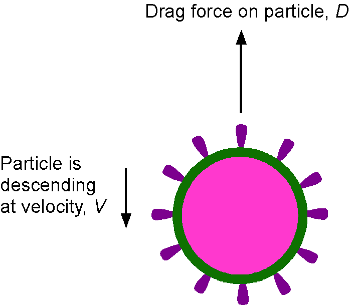
1. Let  . The relationship between the settling velocity and other properties can be written in the general functional form as
![\[ V = f \left( D_p, \mu, g, \Delta \varrho \right) \]](https://eaglepubs.erau.edu/app/uploads/quicklatex/quicklatex.com-8cfd7f9fcb512d35484403571affe711_l3.svg "Rendered by QuickLaTeX.com")
and in implicit form
![\[ g \left( V, D_p, \mu, g, \Delta \varrho \right) = 0 \]](https://eaglepubs.erau.edu/app/uploads/quicklatex/quicklatex.com-d5f2060af26d43bbaa7b6214e99ad004_l3.svg "Rendered by QuickLaTeX.com")
2. and ; there are 3 fundamental dimensions in this problem. Therefore, , so there are two products.
3. For each variable, the dimensions are
![\begin{eqnarray*} \left[ V \right] & = &\rm LT^{-1} \\ \left[ D_p \right] & = &\rm L \\ \left[ \mu \right] & = & \rm M L^{-1} T^{-1} \\ \left[ g \right] & = & \rm L T^{-2} \\ \left[ \Delta \varrho \right] & = &\rm M L^{-3} \end{eqnarray*}](https://eaglepubs.erau.edu/app/uploads/quicklatex/quicklatex.com-48ba35bf8304512fd6d7a2276c7813d6_l3.svg "Rendered by QuickLaTeX.com")
4. The dimensional matrix is
![\[ \begin{array}{l|r|r|r|r|r|r} \mbox{\small Base~unit} & V & D_p & \mu & g & \Delta \varrho \\ \hline \text{\small Mass M:} & 0 & 0 & 1 & 0 & 1 \\ \text{\small Length L:} & 1 & 1 & -1 & 1 & -3 \\ \text{\small Time T:} & -1 & 0 & -1 & -2 & 0 \end{array} \]](https://eaglepubs.erau.edu/app/uploads/quicklatex/quicklatex.com-3beb873995b3f62cb5f53f01fcfe3575_l3.svg "Rendered by QuickLaTeX.com")
5. The parameters , , and are to be chosen as the repeating variables, which will primarily affect the settling velocity. They also collectively include all the fundamental dimensions. Finding the determinant of the dimensional submatrix that is formed by the repeating variables shows that
![\[ \det \begin{bmatrix} 0 & 1 & 0 \\ 1 & -1 & 1 \\ 0 & -1 & -2 \end{bmatrix} \ne 0 \]](https://eaglepubs.erau.edu/app/uploads/quicklatex/quicklatex.com-2d03b6c9f6d4d69fc5938db061cad64d_l3.svg "Rendered by QuickLaTeX.com")
so the selected repeating variables are linearly independent.
The objective is to find the grouping that involves , so
![\[ \Pi_{1} = (D_p)^{\alpha} (\mu)^{\beta} (g)^{\gamma} \, V \]](https://eaglepubs.erau.edu/app/uploads/quicklatex/quicklatex.com-b0033456c295561cbc411dc2ea660d2d_l3.svg "Rendered by QuickLaTeX.com")
In terms of the dimensions of the parameters, then
![\[ \left[ \Pi_{1} \right] = 1 = \rm M^{0}L^{0}T^{0} = \rm \left( L \right)^{\alpha} \left( M L^{-1} T^{-1} \right)^{\beta} \left( L T^{-2} \right)^{\gamma} \left(LT^{-1} \right) \]](https://eaglepubs.erau.edu/app/uploads/quicklatex/quicklatex.com-c38d0b9b02a944687a524435309f6109_l3.svg "Rendered by QuickLaTeX.com")
For to be dimensionless, then the powers or exponents of M, L, and T must add to zero, i.e.,
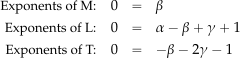
By inspection ,  and
and  so
so
![\[ \Pi_{1} = (D_p)^{\alpha} (\mu)^{\beta} (g)^{\gamma} \, V = (D_p)^{-1/2} (\mu)^{0} (g)^{-1/2} \, V \]](https://eaglepubs.erau.edu/app/uploads/quicklatex/quicklatex.com-c193ec4c9fd898123c100e05529d653f_l3.svg "Rendered by QuickLaTeX.com")
or
![\[ \Pi_{1} = \frac{V}{\sqrt{D_p \, g}} \]](https://eaglepubs.erau.edu/app/uploads/quicklatex/quicklatex.com-3688f02b9bc9e8cf796361ff009090d0_l3.svg "Rendered by QuickLaTeX.com")
Worked Example #33
A weir is an obstruction in an open channel water flow. The volume flow rate over the weir depends on acceleration under gravity , the width of the weir  (into the screen), and the water height
  above the weir.
- Write out the functional relationship in explicit and implicit form.
- How many fundamental (base) dimensions are involved?
- Write out the dimensional matrix for this problem.
- Determine the groupings that govern this problem.
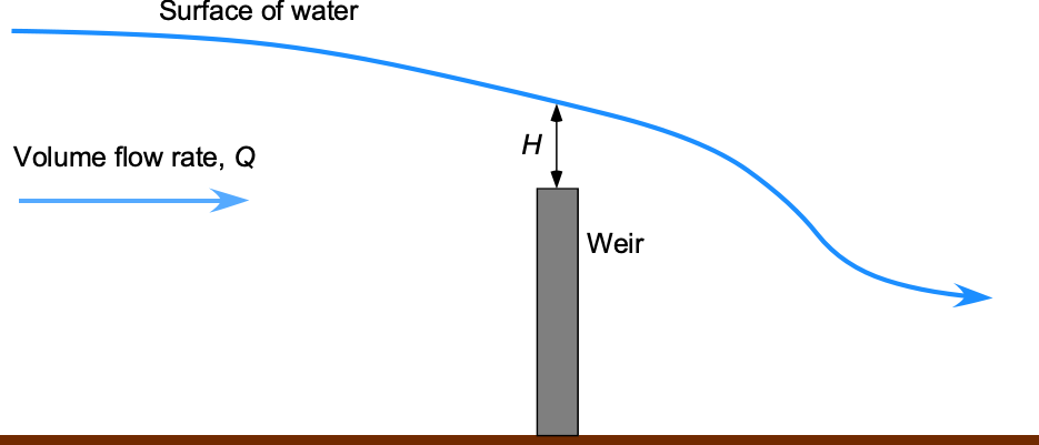
1. The explicit form of the relationship is
![\[ Q = f( g, b, H ) \]](https://eaglepubs.erau.edu/app/uploads/quicklatex/quicklatex.com-3c5ceec2eb53e5754f3cdd2284c03c25_l3.svg "Rendered by QuickLaTeX.com")
and in implicit form, then
![\[ g( Q, g, b, H) = 0 \]](https://eaglepubs.erau.edu/app/uploads/quicklatex/quicklatex.com-4f547e38182d9af7e2ee1b4c5aa52784_l3.svg "Rendered by QuickLaTeX.com")
2. In this problem, there are only two base dimensions, length and time , so the procedure should be more straightforward.
The units involved are
![\begin{eqnarray*} \left[ Q \right] & = & \rm L^3 T^{-1} \\ \left[ g \right] & = & \rm L T^{-2} \\ \left[ b \right] & = &\rm L \\ \left[ H \right] & = & \rm L \end{eqnarray*}](https://eaglepubs.erau.edu/app/uploads/quicklatex/quicklatex.com-22b49532ab20965fec2e79af2cbd187c_l3.svg "Rendered by QuickLaTeX.com")
3. The dimensional matrix is
![\[ \begin{array}{l|r|r|r|r|r|r} \mbox{\small Base~unit} & Q & g & b & H \\ \hline \text{\small Length L:} & 3 & 1 & 1 & 1 \\ \text{\small Time T:} & -1 & -2 & 0 & 0 \end{array} \]](https://eaglepubs.erau.edu/app/uploads/quicklatex/quicklatex.com-4555d11e1dabd13e63cb8286cfd0b28e_l3.svg "Rendered by QuickLaTeX.com")
4. There will be two products because the number of the basic quantities and number of variables in this problem . and can be used as repeating variables, which collectively include all the fundamental dimensions and are linearly independent. Note: Both and cannot be chosen as repeating variables because they have the same units and are not linearly independent.
For the first product then
![\[ \Pi_{1} = (g)^{\alpha} (H)^{\beta} Q \]](https://eaglepubs.erau.edu/app/uploads/quicklatex/quicklatex.com-8d897c27a4fde6ae9d00e45b563a918d_l3.svg "Rendered by QuickLaTeX.com")
In terms of the dimensions of the parameters, then
![\[ \left[ \Pi_{1} \right] = 1 = \rm L^{0}T^{0} = \rm \left( L T^{-2} \right)^{\alpha} \left( L \right)^{\beta} \left( L ^3T^{-1} \right) \]](https://eaglepubs.erau.edu/app/uploads/quicklatex/quicklatex.com-440ee4c1def991df7e88636633088deb_l3.svg "Rendered by QuickLaTeX.com")
For to be dimensionless, then the powers or exponents of and must add to zero, i.e.,

By inspection and  so the grouping is
![\[ \Pi_{1} = (g)^{\alpha} (H)^{\beta} (g) Q = (g)^{-1/2} (H)^{-5/2} \, Q \]](https://eaglepubs.erau.edu/app/uploads/quicklatex/quicklatex.com-3de8befcd3f5ffe5e4e24a069e3eaeeb_l3.svg "Rendered by QuickLaTeX.com")
or
![\[ \Pi_{1} =\frac{Q} {g^{1/2} \, H^{5/2}} \]](https://eaglepubs.erau.edu/app/uploads/quicklatex/quicklatex.com-2bf25300abafb00da3a1348be3812376_l3.svg "Rendered by QuickLaTeX.com")
For the second product then
![\[ \Pi_{2} = (g)^{\alpha} (H)^{\beta} b \]](https://eaglepubs.erau.edu/app/uploads/quicklatex/quicklatex.com-6910d56bbdfe06543fffc3aa9abb5773_l3.svg "Rendered by QuickLaTeX.com")
In terms of the dimensions of the parameters, then
![\[ \left[ \Pi_{2} \right] = 1 = \rm L^{0}T^{0} = \rm \left( L T^{-2} \right)^{\alpha} \left( L \right)^{\beta} \left( L \right) \]](https://eaglepubs.erau.edu/app/uploads/quicklatex/quicklatex.com-c0e9146dc3e04686d6e61e9213f02228_l3.svg "Rendered by QuickLaTeX.com")
For to be dimensionless, then the powers or exponents of and must add to zero, i.e.,
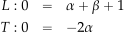
By inspection and so the grouping is
![\[ \Pi_{2} = (g)^{0} (H)^{-1} b = \frac{b}{H} \]](https://eaglepubs.erau.edu/app/uploads/quicklatex/quicklatex.com-6eff95ea2d5c52c465e0333b7f209482_l3.svg "Rendered by QuickLaTeX.com")
Therefore, the result is
![\[ \phi_1 \left( \frac{Q} {g^{1/2} \, H^{5/2}}, \frac{b}{H} \right) = 0 \]](https://eaglepubs.erau.edu/app/uploads/quicklatex/quicklatex.com-aaa4efd92a4328714519b251f06d226e_l3.svg "Rendered by QuickLaTeX.com")
or
![\[ \left( \frac{Q} {g^{1/2} \, H^{5/2}} \right) = \phi_2 \left( \frac{b}{H} \right) \]](https://eaglepubs.erau.edu/app/uploads/quicklatex/quicklatex.com-75d1742f2563cabd3d0cb0891feb22a5_l3.svg "Rendered by QuickLaTeX.com")
Worked Example #34
Sir Geoffrey I. Taylor (1886–1975) was a British physicist and engineer. He used dimensional analysis to estimate an explosion’s blast wave propagation characteristics. Taylor assumed that the radius of the wave was a function of the energy released during the explosion, the density of the air , and the time  . Using the Buckingham Pi method, recreate Taylor’s steps and find the dimensionless grouping that governs this behavior. How does the radius of the blast wave change by a doubling of (i) and (ii) time?
The relationship may be written in a general functional form as
![\[ R = \phi \left( E, \varrho, t \right) \]](https://eaglepubs.erau.edu/app/uploads/quicklatex/quicklatex.com-1c2b3b1af093ae4f754697efea4070b7_l3.svg "Rendered by QuickLaTeX.com")
or in implicit form, then
![\[ \phi_1 \left(R, E, \varrho, t \right) = 0 \]](https://eaglepubs.erau.edu/app/uploads/quicklatex/quicklatex.com-a3705f543e9c2b6588ed07b6001c9ed5_l3.svg "Rendered by QuickLaTeX.com")
Therefore, and because the problem includes the dimensions of mass, length, and time, and so there is just one product. Energy is the ability to do work, so the dimensions of energy will be the same as those of work, equivalent to a force times a distance, i.e.,  . Setting up the dimensional matrix gives
![\[ \begin{array}{l|c|r|r|r} \mbox{\small Base~unit} & R & E & \varrho & t \\ \hline \text{\small Mass M:} & 0 & 1 & 1 & 0 \\ \text{\small Length L:} & 1 & 2 & -3 & 0 \\ \text{\small Time T:} & 0 & -2 & 0 & 1 \end{array} \]](https://eaglepubs.erau.edu/app/uploads/quicklatex/quicklatex.com-5d691caa9e80354cee14f5c5780c10b6_l3.svg "Rendered by QuickLaTeX.com")
Following the Buckingham method, then the product is
![\[ \Pi = (E)^{\alpha} (\varrho)^{\beta} (t)^{\gamma} \, R \]](https://eaglepubs.erau.edu/app/uploads/quicklatex/quicklatex.com-448d4176652b3518bd287cd0fd84caa9_l3.svg "Rendered by QuickLaTeX.com")
where the specific values of the coefficients , and must be obtained to make the equation dimensionally homogeneous. In terms of the dimensions of the parameters, then
![\[ \left[ \Pi \right] = 1 = \rm M^{0}L^{0}T^{0} = \rm \left( M L^2 T^{-2} \right)^{\alpha} \left( M L^{-3} \right)^{\beta} \left(T \right)^{\gamma} \, L \]](https://eaglepubs.erau.edu/app/uploads/quicklatex/quicklatex.com-7dd8b1b0048bf5417a5b3a4489a2f1c3_l3.svg "Rendered by QuickLaTeX.com")
For to be dimensionless, then the powers or exponents of , , and must add to zero, i.e.,
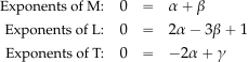
In this case,  , so
, so  from the second equation. This further gives that
  , and
, and  . Therefore,
![\[ \Pi = (E)^{\alpha} (\varrho)^{\beta} (t)^{\gamma} \, R = E^{-1/5} \varrho^{1/5} t^{-2/5} R \]](https://eaglepubs.erau.edu/app/uploads/quicklatex/quicklatex.com-7bace2a51b59b002be7390c6e97bd2f5_l3.svg "Rendered by QuickLaTeX.com")
or
![\[ \Pi = \frac{ R \, \varrho^{1/5}}{E^{1/5} \, t^{2/5}} \]](https://eaglepubs.erau.edu/app/uploads/quicklatex/quicklatex.com-f6aa904a601b3b0fabecf4ea2dcc13bf_l3.svg "Rendered by QuickLaTeX.com")
In the final form, then
![\[ R = \phi_2 \left( \frac{E^{1/5} \, t^{2/5}}{\varrho^{1/5}} \right) \]](https://eaglepubs.erau.edu/app/uploads/quicklatex/quicklatex.com-aa025f1bfa6c42660364dd098394c235_l3.svg "Rendered by QuickLaTeX.com")
In the second part, the question is how the radius of the blast wave changes by a doubling of . According to the derived relationship, the radius would increase by  or about 1.15. By doubling the time, then the radius of the wave would increase by a factor of
  or about 1.32.
Worked Example #35
An ocean surface wave is a sinusoidal-like disturbance propagating along the ocean’s surface, as shown in the figure below. The speed of the wave,  , is found to be a function of the surface tension of the seawater, , the density of the seawater, , and the wavelength,
  , of the wave.
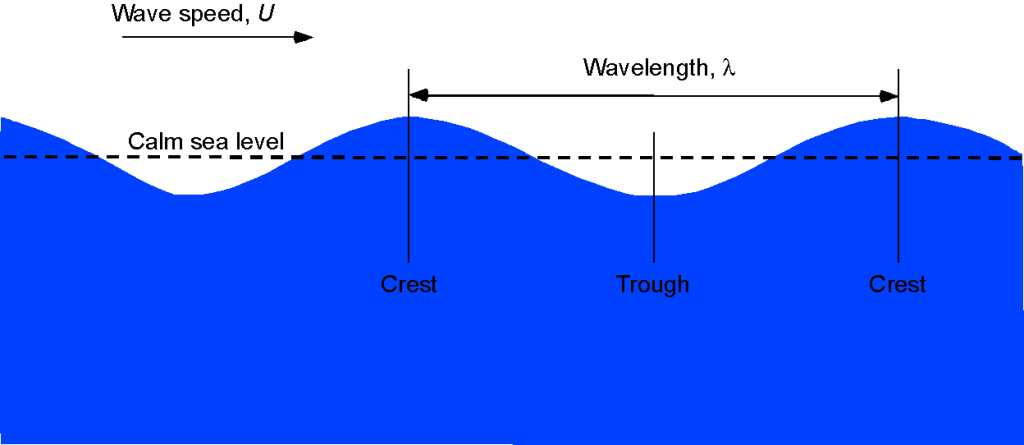 1. Write down the functional relationship for the speed of the wave in terms of the given parameters, in both implicit and explicit form.
2. How many base dimensions and groupings are involved in this problem?
3. Write down the dimensions of all the parameters in base dimensions. Notice: The units of surface tension are expressed as a force per unit area.
4. Create the dimensional matrix for this problem.
5. Determine the dimensionless parameter(s) that describe this problem.
1. In explicit form, the speed of the wave is
![\[ U = f(\sigma,\, \varrho, \lambda) \]](https://eaglepubs.erau.edu/app/uploads/quicklatex/quicklatex.com-8f618505a14c970ea0d6e11d1168a4e6_l3.svg "Rendered by QuickLaTeX.com")
where is some function. In implicit form, then
![\[ g( \sigma,\, \varrho,\, \lambda, U) = 0 \]](https://eaglepubs.erau.edu/app/uploads/quicklatex/quicklatex.com-322e99d0041fbf39b968abe4d925278b_l3.svg "Rendered by QuickLaTeX.com")
where is some other function.
2. The base dimensions and groupings involved in this problem are:
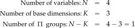
3. Below are the dimensions of all the parameters in this problem in terms of base dimensions:
The speed of the wave, , has base dimensions of
![\[ \left[ U \right] = \rm L T^{-1} \]](https://eaglepubs.erau.edu/app/uploads/quicklatex/quicklatex.com-09d95ad8ae618012750077b10c881701_l3.svg "Rendered by QuickLaTeX.com")
Surface tension, , is given in the question as a “force per unit area,” so it has base dimensions of
![\[ \left[ \sigma \right] = \rm ( M L T^{-2}) L^{-2} = \rm M L^{-1} T^{-2} \]](https://eaglepubs.erau.edu/app/uploads/quicklatex/quicklatex.com-63e5c62918e88f4060cb12b583c2818a_l3.svg "Rendered by QuickLaTeX.com")
Density, , has base dimensions of
![\[ \left[ \varrho \right] = \rm M \, L^{-3} \]](https://eaglepubs.erau.edu/app/uploads/quicklatex/quicklatex.com-7c7f84885304a08ac7895b55f2b2cfba_l3.svg "Rendered by QuickLaTeX.com")
Wavelength, , has base dimensions of
![\[ \left[ \lambda \right] =\rm L \]](https://eaglepubs.erau.edu/app/uploads/quicklatex/quicklatex.com-81af6e5929060c768471dd57aac1f159_l3.svg "Rendered by QuickLaTeX.com")
4. From the previous results, the dimensional matrix is
![\[ \begin{array}{l|r|r|r|r|r|r} \mbox{\small Base~unit} & \sigma & \varrho & \lambda & U \\ \hline \text{\small Mass M:} & 1 & 1 & 0 & 0 \\ \text{\small Length L:} & -1 & -3 & 1 & 1 \\ \text{\small Time T:} & -2 & 0 & 0 & -1 \end{array} \]](https://eaglepubs.erau.edu/app/uploads/quicklatex/quicklatex.com-f15e9cf770f6868d26d200d6526530a8_l3.svg "Rendered by QuickLaTeX.com")
5. The wave speed cannot be a repeating variable, so the only possible choice of the repeating variables is , , and . Finding the determinant of the dimensional submatrix that is formed by the repeating variables shows that
![\[ \det \begin{bmatrix} 1 & 1 & 0 \\ -1 & -3 & 1 \\ -2 & 0 & 0 \end{bmatrix} \ne 0 \]](https://eaglepubs.erau.edu/app/uploads/quicklatex/quicklatex.com-951ef74eac98ec3297261c91f2e098c4_l3.svg "Rendered by QuickLaTeX.com")
so the selected repeating variables are linearly independent.
The group will be
![\[ \Pi_1 = g_1 (\sigma, \, \varrho, \, \lambda, \, U) \]](https://eaglepubs.erau.edu/app/uploads/quicklatex/quicklatex.com-0e4f729318c3f875c94cf7e67a2bb229_l3.svg "Rendered by QuickLaTeX.com")
Therefore,
![\[ \left[ \Pi_1 \right] = 1 = \rm M^ 0 \, L^0 \, T^0 = \rm \sigma^{\alpha} \, \varrho^{\beta} \, \lambda^{\gamma} \, U \]](https://eaglepubs.erau.edu/app/uploads/quicklatex/quicklatex.com-00a20e312740d0eb01d74984e22b49e7_l3.svg "Rendered by QuickLaTeX.com")
In terms of dimensions, then
![\[, \left[ \Pi_1 \right] = 1 = \rm M^0 \, L^0 \, T^0 = \rm ( M L^{-1} T^{-2})^{\alpha} \, (ML^{-3})^{\beta} \ (L)^{\gamma} \, LT^{-1} \]](https://eaglepubs.erau.edu/app/uploads/quicklatex/quicklatex.com-795325bb50945097536d03c8f33296aa_l3.svg "Rendered by QuickLaTeX.com")
Alternatively, the preceding can be written as
![\[ \rm M^0 \, L^0 \, T^0 = \rm M^{(\alpha + \beta)} \, L^{(-3\beta + \gamma + 1)} \, T^{(-2\alpha - 1)} \]](https://eaglepubs.erau.edu/app/uploads/quicklatex/quicklatex.com-5fd2ef2b2a8d55ab5b0f4db0c1afdd60_l3.svg "Rendered by QuickLaTeX.com")
For this equation to be mathematically balanced on the left and right sides, i.e., to be dimensionally homogeneous, then
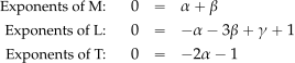
Solving the foregoing equations gives , , so that the resulting grouping is
![\[ \Pi_1 = \sigma^{-1/2} \ \varrho^{1/2} \, \lambda^{0} \, U \]](https://eaglepubs.erau.edu/app/uploads/quicklatex/quicklatex.com-3ed97bc50041e479caff1a8f82600856_l3.svg "Rendered by QuickLaTeX.com")
or
![\[ \Pi_1 = U \sqrt{\frac{\varrho} {\sigma }} \]](https://eaglepubs.erau.edu/app/uploads/quicklatex/quicklatex.com-3575ede86dbbb0366300603da0817791_l3.svg "Rendered by QuickLaTeX.com")
As a final check, it is easy to show that this grouping is dimensionless because
![\[ \left[ \Pi_1 \right] = \mathrm{L\,T^{-1}} \left( \frac{ \mathrm{M\,L^{-3}} }{ \mathrm{M\,L^{-1}\,T^{-2}} } \right)^{1/2} = \mathrm{L\,T^{-1}} \left( \mathrm{L^{-2}\,T^{2}} \right)^{1/2} = \mathrm{L\,T^{-1}\,L^{-1}\,T} = 1 \]](https://eaglepubs.erau.edu/app/uploads/quicklatex/quicklatex.com-698bd4dfb673090d72d2d611440da6c2_l3.svg "Rendered by QuickLaTeX.com")
Notice that the dimensionless group
![\[ \Pi_1 = U \sqrt{ \frac{ \varrho }{ \sigma } } \]](https://eaglepubs.erau.edu/app/uploads/quicklatex/quicklatex.com-9d5f0987f1d127f923bae56468627f3b_l3.svg "Rendered by QuickLaTeX.com")
compares the wave speed to a characteristic speed scale defined by surface tension and density. Its inverse,
![\[ \sqrt{ \frac{ \sigma }{ \varrho } } \]](https://eaglepubs.erau.edu/app/uploads/quicklatex/quicklatex.com-42912f2dc383ceeda01fdc752b80f0fa_l3.svg "Rendered by QuickLaTeX.com")
has the units of velocity and represents a characteristic wave speed for disturbances dominated by surface tension.
This grouping does not have a widely used standalone name, but it appears frequently in the study of capillary waves. It is, therefore, interpreted as a non-dimensional wave speed for surface-tension-driven phenomena. In fact, from capillary wave theory, the wave speed scales as
![\[ U \sim \sqrt{ \frac{ \sigma }{ \varrho \lambda } } \]](https://eaglepubs.erau.edu/app/uploads/quicklatex/quicklatex.com-cea850c396ad2a116fc82d9e8de11d95_l3.svg "Rendered by QuickLaTeX.com")
which shows that the speed increases with surface tension , and decreases with wavelength and density . The group captures this balance in non-dimensional form and is used to characterize regimes where capillary forces dominate over gravitational or viscous effects.
In contrast to capillary waves, which are driven by surface tension, longer-wavelength surface waves are typically dominated by gravity. In this regime, the wave speed scales with gravitational acceleration and wavelength as
![\[ U \sim \sqrt{g \lambda} \]](https://eaglepubs.erau.edu/app/uploads/quicklatex/quicklatex.com-e9af7be839994a7007869b0265781760_l3.svg "Rendered by QuickLaTeX.com")
This comes from the dispersion relation for gravity waves in deep water, where surface tension is negligible compared to gravitational restoring forces. The corresponding dimensionless group for gravity waves is
![\[ \Pi_2 = \frac{U}{\sqrt{g \lambda}} \]](https://eaglepubs.erau.edu/app/uploads/quicklatex/quicklatex.com-39c588d0e9a9c8c289c1b95cb57db0b5_l3.svg "Rendered by QuickLaTeX.com")
This group compares the actual wave speed to the characteristic gravity wave speed, and is commonly encountered in ocean wave modeling, ship hydrodynamics, and coastal engineering.
Worked Example #36
The flow rate in a pipe is to be measured with an orifice plate, as shown in the figure below. The static pressure before and after the plate is measured using two pressure gauges. The volumetric flow rate is found to be a function of the measured pressure drop across the plate,  , the fluid density, , the pipe diameter, , and the orifice diameter, .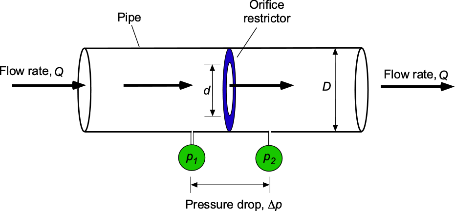
- Write down the functional relationship for the volumetric flow rate in terms of the other parameters, in both implicit and explicit form.
- Write down the base dimensions of the parameters involved in this problem.
- How many base dimensions and dimensionless groupings are involved in this problem?
- Write out the dimensional matrix for this problem.
- Choose the repeating variables and explain your choice.
- Determine the dimensionless grouping(s) for the parameters involved.
- Write down the final dimensionless functional relationship(s).
1. The volumetric flow rate of water can be written in an explicit form as
![\[ Q = \phi_1 (\Delta p, \varrho, D, d) \]](https://eaglepubs.erau.edu/app/uploads/quicklatex/quicklatex.com-1a71a3b5c217a71d4b7aaad3d60d8844_l3.svg "Rendered by QuickLaTeX.com")
where is some function, and in the implicit form as
![\[ \phi_2 (Q, \Delta p, \varrho, D, d) = 0 \]](https://eaglepubs.erau.edu/app/uploads/quicklatex/quicklatex.com-39eb4953dcef9c3de45568423d5a41f5_l3.svg "Rendered by QuickLaTeX.com")
where  is some other function.
2. The dimensions of the parameters involved are:
![\left[ Q \right] =\rm L^3 T^{-1}](https://eaglepubs.erau.edu/app/uploads/quicklatex/quicklatex.com-8b5d9e71540582880a557a12dd3f41aa_l3.svg "Rendered by QuickLaTeX.com")
![\left[ \Delta p \right] = \rm ( M L T^{-2} ) L^{-2} = M L^{-1} T^{-2}](https://eaglepubs.erau.edu/app/uploads/quicklatex/quicklatex.com-60d96aa80f08d75a7c8fc1fe0d1555bc_l3.svg "Rendered by QuickLaTeX.com")
![\left[ \varrho \right] =\rm M L^{-3}](https://eaglepubs.erau.edu/app/uploads/quicklatex/quicklatex.com-da131b2d97641d03048873efc8fb4dd9_l3.svg "Rendered by QuickLaTeX.com")
![\left[ D \right] = \rm L](https://eaglepubs.erau.edu/app/uploads/quicklatex/quicklatex.com-167f702e1acee9f8d06240add4f92946_l3.svg "Rendered by QuickLaTeX.com")
![\left[ d \right] = \rm L](https://eaglepubs.erau.edu/app/uploads/quicklatex/quicklatex.com-27a119426ba95ce9c84a387083e3affa_l3.svg "Rendered by QuickLaTeX.com")
3. The number of base dimensions and groupings involved in this problem:
- Number of variables: .
- Number of base dimensions (mass, length, and time are all involved): .
- Number of groups:
 .
.
4. The dimensional matrix is
![\[ \begin{array}{l|r|r|r|r|r|r|r} \mbox{\small Base~unit} & Q & \Delta p & \varrho & D & d \\ \hline \text{\small Mass M:} & 0 & 1 & 1 & 0 & 0 \\ \text{\small Length L:} & 3 & -1 & -3 & 1 & 1 \\ \text{\small Time T:} & -1 & -2 & 0 & 0 & 0 \end{array} \]](https://eaglepubs.erau.edu/app/uploads/quicklatex/quicklatex.com-a51f0b0202cc20dd685bc6061e8afc99_l3.svg "Rendered by QuickLaTeX.com")
5. The only possible choice of repeating variables are , , , and . Both and cannot be chosen as repeating variables because they are not linearly independent. But one or the other should be chosen so can be chosen, and the repeating variables will be , , and . Finding the determinant of the dimensional submatrix that is formed by the repeating variables shows that
so the selected repeating variables are linearly independent.
6. The groups will be formed from
![\[ \Pi_1 = g_1(\Delta p, \varrho, D, Q) \]](https://eaglepubs.erau.edu/app/uploads/quicklatex/quicklatex.com-bbd39548323fffc2bf3b7a2a54034c3c_l3.svg "Rendered by QuickLaTeX.com")
and
![\[ \Pi_2 = g_2( \Delta p, \varrho, D, d) \]](https://eaglepubs.erau.edu/app/uploads/quicklatex/quicklatex.com-1df42ffbad3ba83b05a2a06c1d14709f_l3.svg "Rendered by QuickLaTeX.com")
The dimensionless groupings must now be determined.
For then:
so
![\[ \left[ \Pi_1 \right] = 1 = \rm M^0 L^0 T^0 = ( \Delta p)^{\alpha} \, ( \varrho)^{\beta} \, (D)^{\gamma} \, Q \]](https://eaglepubs.erau.edu/app/uploads/quicklatex/quicklatex.com-031adbb179ef514f07bddaf173548392_l3.svg "Rendered by QuickLaTeX.com")
and inserting the dimensions for each parameter gives
![\[ \left[ \Pi_1 \right] = 1 = \rm M^0 L^0 T^0 =\rm (M L^{-1} T^{-2} )^{\alpha} \, (M L^{-3})^{\beta}\, (L)^{\gamma} \, L^3 T^{-1} \]](https://eaglepubs.erau.edu/app/uploads/quicklatex/quicklatex.com-6b07bc8fe782c7d7cbd3553cc8b7b78e_l3.svg "Rendered by QuickLaTeX.com")
or
![\[ \left[ \Pi_1 \right] = 1 = \rm ^0 L^0 T^0 = \rm M^{(\alpha+\beta)} \, L^{(-\alpha -3\beta + \gamma+3)} \, T^{(-2\alpha - 1)} \]](https://eaglepubs.erau.edu/app/uploads/quicklatex/quicklatex.com-fa92029a2cf7d0eb8d03cba88b0433d9_l3.svg "Rendered by QuickLaTeX.com")
For to be dimensionless, the powers must add to zero, i.e.,
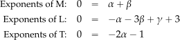
Solving the equations gives , , and . This means, therefore, that is
![\[ \Pi_1 =\Delta p^{-1/2} \, \varrho^{1/2} \, D^{-2} \, Q \]](https://eaglepubs.erau.edu/app/uploads/quicklatex/quicklatex.com-58cb68298ecd024c67075e284e300d02_l3.svg "Rendered by QuickLaTeX.com")
or
![\[ \Pi_1 = Q \, \sqrt{ \frac{\varrho}{\Delta p \, D^{4}}} \]](https://eaglepubs.erau.edu/app/uploads/quicklatex/quicklatex.com-f59567b978ff64340b2cbbd798b0a608_l3.svg "Rendered by QuickLaTeX.com")
To check if this is a dimensionless grouping, substitute the dimensions of the parameters, i.e.,
![\[ \left[ \Pi_1 \right] = \rm L^3 T^{-1} \left( \frac{M L^{-3}}{M L^{-1} T^{-2} L^4} \right)^{-1/2} = \rm L^3 T^{-1} \left( \frac{L^{-6}}{T^{-2}} \right)^{-1/2} = L^3 T^{-1} L^{-3} T = 1 \]](https://eaglepubs.erau.edu/app/uploads/quicklatex/quicklatex.com-b75ec538d9a2a5bcab2d75864ec8c602_l3.svg "Rendered by QuickLaTeX.com")
so confirming that the grouping is indeed dimensionless.
For then:
![\[ \Pi_2 = g_1(\Delta p, \varrho, D, d) \]](https://eaglepubs.erau.edu/app/uploads/quicklatex/quicklatex.com-29da65ab73d1f0e78c64cad5fb205be9_l3.svg "Rendered by QuickLaTeX.com")
so
![\[ \left[ \Pi_2 \right] = 1 = \rm M^0 L^0 T^0 = ( \Delta p)^{\alpha} \, ( \varrho)^{\beta} \, (D)^{\gamma} \, d \]](https://eaglepubs.erau.edu/app/uploads/quicklatex/quicklatex.com-923cccf86acd338de9a9dd61463f11a3_l3.svg "Rendered by QuickLaTeX.com")
and inserting the dimensions for each parameter gives
![\[ \left[ \Pi_2 \right] = 1 = \rm M^0 L^0 T^0 = \rm (M L^{-1} T^{-2} )^{\alpha} \, (M L^{-3})^{\beta}\, (L)^{\gamma} \, L \]](https://eaglepubs.erau.edu/app/uploads/quicklatex/quicklatex.com-b17f2d9e340167e522bd3faae446dcbe_l3.svg "Rendered by QuickLaTeX.com")
or
![\[ \left[ \Pi_2 \right] = 1 = \rm M^0 L^0 T^0 = \rm M^{(\alpha+\beta)} \, L^{(-\alpha -3\beta + \gamma+1)} \, T^{(-2\alpha)} \]](https://eaglepubs.erau.edu/app/uploads/quicklatex/quicklatex.com-744fa07dadaed607781ca335de80d1a7_l3.svg "Rendered by QuickLaTeX.com")
For to be dimensionless, the powers must add to zero, i.e.,
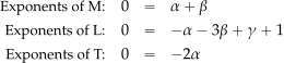
Solving the equations gives , , and . This means, therefore, that is
![\[ \Pi_2 = \Delta p^{0} \, \varrho^{0} \, D^{-1} \, d = \frac{d}{D} \]](https://eaglepubs.erau.edu/app/uploads/quicklatex/quicklatex.com-4a936d0929a503617dae05335e985089_l3.svg "Rendered by QuickLaTeX.com")
In this case, the ratio of one length to another is dimensionless.
7. Finally, the dimensionless relationship between the volumetric flow rate and the other parameters is
![\[ Q \, \sqrt{ \frac{\varrho}{\Delta p \, D^{4}}} = \phi \left( \frac{d}{D} \right) \]](https://eaglepubs.erau.edu/app/uploads/quicklatex/quicklatex.com-dfdc26d824229af9a4943f1c46a53106_l3.svg "Rendered by QuickLaTeX.com")
Worked Example #37 – Air jet
An air jet holds a ball in vertical equilibrium, as shown in the figure below. The equilibrium height, , depends on the diameter of the ball, , jet diameter, , the ball’s weight, , the viscosity of air, , the density of air, , and the flow velocity, . If the final dimensionless relationship can be written as
![\[ \frac{h}{D} = \psi \left( \frac{\varrho V D}{\mu}, \, \Pi_3, \, \Pi_4 \right) \]](https://eaglepubs.erau.edu/app/uploads/quicklatex/quicklatex.com-e6b957313e190c0bb515f1b92156a06b_l3.svg "Rendered by QuickLaTeX.com")
then determine the two remaining groups. Confirm that your groups are dimensionless.
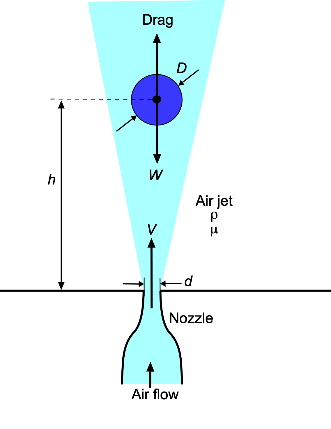
The relationship may be written in a general functional form as
![\[ h = \phi_1 \left( D, d, W, \mu, \varrho, V \right) \]](https://eaglepubs.erau.edu/app/uploads/quicklatex/quicklatex.com-332381e061c169eb47d1f388bb440632_l3.svg "Rendered by QuickLaTeX.com")
or in the implicit form as
![\[ \phi_2 \left( h. D, d, W, \mu, \varrho, V \right) = 0 \]](https://eaglepubs.erau.edu/app/uploads/quicklatex/quicklatex.com-ddc1dd28a74a282670eb30bd21af24df_l3.svg "Rendered by QuickLaTeX.com")
The base dimensions are:
![\[ \left[ D \right] = \rm L \]](https://eaglepubs.erau.edu/app/uploads/quicklatex/quicklatex.com-a073b8ba0a2985992abaa2022e19ee02_l3.svg "Rendered by QuickLaTeX.com")
![\[ \left[ d \right] = \rm L \]](https://eaglepubs.erau.edu/app/uploads/quicklatex/quicklatex.com-ff1f946168166d3715859f6ca3b41b3f_l3.svg "Rendered by QuickLaTeX.com")
![\[ \left[ W \right] = \rm M L T^{-2} \]](https://eaglepubs.erau.edu/app/uploads/quicklatex/quicklatex.com-2b2e50ab1c5f387b2eb645428472cfff_l3.svg "Rendered by QuickLaTeX.com")
![\[ \left[ \mu \right] = \rm M L^{-1} T^{-1} \]](https://eaglepubs.erau.edu/app/uploads/quicklatex/quicklatex.com-79079be4bb8238037f04e419f9229f2b_l3.svg "Rendered by QuickLaTeX.com")
![\[ \left[ \varrho \right] = \rm M L^{-3} \]](https://eaglepubs.erau.edu/app/uploads/quicklatex/quicklatex.com-46e9b7c9121ff0b0368d21adc7c6b144_l3.svg "Rendered by QuickLaTeX.com")
![\[ \left[ V \right] = \rm L T^{-1} \]](https://eaglepubs.erau.edu/app/uploads/quicklatex/quicklatex.com-819857c07879e8c00dfaf277893d1006_l3.svg "Rendered by QuickLaTeX.com")
Setting up the dimensional matrix gives
![\[ \begin{array}{l|c|r|r|r|r|r|r} \mbox{\small Base~unit} & h & D & d & W & \mu & \varrho & V \\ \hline \text{\small Mass M:} \quad & 0& 0 & 0 & 1 & 1 & 1 & 0 \\ \text{\small Length L:} \quad & 1 & 1 & 1 & 1 & -1 & -3 & 1 \\ \text{\small Time T:} \quad & 0 & 0 & 0 & -1 & -1 & 0 & -1 \end{array} \]](https://eaglepubs.erau.edu/app/uploads/quicklatex/quicklatex.com-703ef6537e342309a56e713b222f52af_l3.svg "Rendered by QuickLaTeX.com")
The parameters collectively involve mass, length, and time, so . There are seven parameters, so  . Therefore, there are groupings.
The four products will be
![\[ \Pi_1 = \psi_1 \left( \varrho, D, V, h \right) \]](https://eaglepubs.erau.edu/app/uploads/quicklatex/quicklatex.com-637378e9286bb5bf63aca4da1883e4b1_l3.svg "Rendered by QuickLaTeX.com")
![\[ \Pi_2 = \psi_2 \left( \varrho, D, V, \mu \right) \]](https://eaglepubs.erau.edu/app/uploads/quicklatex/quicklatex.com-2de316268f2372d0128f1c1c41fe38cd_l3.svg "Rendered by QuickLaTeX.com")
![\[ \Pi_3 = \psi_3 \left( \varrho, D, V, d \right) \]](https://eaglepubs.erau.edu/app/uploads/quicklatex/quicklatex.com-a4c3c0a546abe07bd9752f75af6f1c10_l3.svg "Rendered by QuickLaTeX.com")
![\[ \Pi_4 = \psi_4 \left( \varrho, D, V, W \right) \]](https://eaglepubs.erau.edu/app/uploads/quicklatex/quicklatex.com-7b0b16e799095103b0689156d9b0a320_l3.svg "Rendered by QuickLaTeX.com")
The information given is that
so only the two groupings involving and need to be determined.
For  then
then
Raising the repeating variables to unknown powers gives for the grouping
![\[ \Pi_3 = (\varrho)^{\alpha} (D)^{\beta} (V)^{\gamma} \, d \]](https://eaglepubs.erau.edu/app/uploads/quicklatex/quicklatex.com-506a2b186488380a0aec37b47ba8f822_l3.svg "Rendered by QuickLaTeX.com")
In terms of dimensions, then
![\[ \left[ \Pi_3 \right] = 1 = \rm M^{0}L^{0}T^{0} = \rm \left( M L^{-3} \right)^{\alpha} \left( L \right)^{\beta} \left(L T^{-1} \right)^{\gamma} \, L \]](https://eaglepubs.erau.edu/app/uploads/quicklatex/quicklatex.com-7a2208d1411131ebe7bf41983fa4a731_l3.svg "Rendered by QuickLaTeX.com")
For to be dimensionless, then
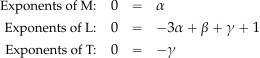
By inspection , , and  , so
, so
![\[ \Pi _3 = (\varrho)^{0} (D)^{-1} (V)^{-2} \, d \]](https://eaglepubs.erau.edu/app/uploads/quicklatex/quicklatex.com-0eff7126998561d3d8319c688bd316e0_l3.svg "Rendered by QuickLaTeX.com")
or
![\[ \Pi_3 = \frac{d}{D} \]](https://eaglepubs.erau.edu/app/uploads/quicklatex/quicklatex.com-7123ec4db86ba493e0daf3b3c99f041b_l3.svg "Rendered by QuickLaTeX.com")
which is a dimensionless length.
Check:
![\[ \left[ \Pi_3 \right] = \frac{L}{L} = 1 \]](https://eaglepubs.erau.edu/app/uploads/quicklatex/quicklatex.com-3e97860b0daf43d8e7b41e1a77a82f4d_l3.svg "Rendered by QuickLaTeX.com")
For  then
then
Raising the repeating variables to unknown powers gives for the grouping
![\[ \Pi_4 = (\varrho)^{\alpha} (D)^{\beta} (V)^{\gamma} \, W \]](https://eaglepubs.erau.edu/app/uploads/quicklatex/quicklatex.com-79055df94b813ab86f1116688447ff09_l3.svg "Rendered by QuickLaTeX.com")
In terms of dimensions, then
![\[ \left[ \Pi_4 \right] = 1 = \rm M^{0}L^{0}T^{0} = \left( M L^{-3} \right)^{\alpha} \left( L \right)^{\beta} \left(L T^{-1} \right)^{\gamma} \, M L T^{-2} \]](https://eaglepubs.erau.edu/app/uploads/quicklatex/quicklatex.com-76f0cce5466f7e9ea1731c6ea01f96ff_l3.svg "Rendered by QuickLaTeX.com")
For to be dimensionless, then
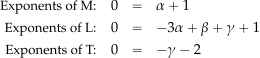
By inspection , , and  , so
, so
![\[ \Pi _4 = (\varrho)^{-1} (D)^{-2} (V)^{-2} \, W \]](https://eaglepubs.erau.edu/app/uploads/quicklatex/quicklatex.com-7e749f1a040c1a8b9bc45c6ba3b5fda5_l3.svg "Rendered by QuickLaTeX.com")
or
![\[ \Pi_4 = \frac{W}{\varrho \, V^2 D^2} \]](https://eaglepubs.erau.edu/app/uploads/quicklatex/quicklatex.com-18041f76a91997ec0e40af20d6e8aadd_l3.svg "Rendered by QuickLaTeX.com")
which is a force coefficient.
Check:
![\[ \left[ \Pi_4 \right] = \frac{\rm M L T^{-2}}{\rm (M L^{-3}) (LT^{-1})^2 (L^2)} = \frac{M L T^{-2}}{M L T^{-2}} = 1 \]](https://eaglepubs.erau.edu/app/uploads/quicklatex/quicklatex.com-33388278a03e2586a6e962da5b59b598_l3.svg "Rendered by QuickLaTeX.com")
Finally, the non-dimensional functional relationship is
![\[ \frac{h}{D} = \psi \left( \frac{\varrho V D}{\mu}, \, \frac{d}{D}, \, \frac{W}{\varrho \, V^2 D^2} \right) \]](https://eaglepubs.erau.edu/app/uploads/quicklatex/quicklatex.com-321eb37e13abd8d4cd299cb36d0a17f5_l3.svg "Rendered by QuickLaTeX.com")
Worked Example #38 – Bobbing booster in the ocean
A solid rocket booster parachutes back to Earth and falls into the sea. The booster bobs around in the sea upright at a frequency of . Using dimensional analysis, show that the dimensionless frequency of this motion,  , is given by
![\[ k = \omega \sqrt{\frac{d}{g}} \]](https://eaglepubs.erau.edu/app/uploads/quicklatex/quicklatex.com-55c88e4ee7533c18d92bb14cce50096f_l3.svg "Rendered by QuickLaTeX.com")
It may be assumed that for this problem, the frequency of motion depends on the diameter of the booster , the mass of the booster,  , the density of the water , and acceleration under gravity, .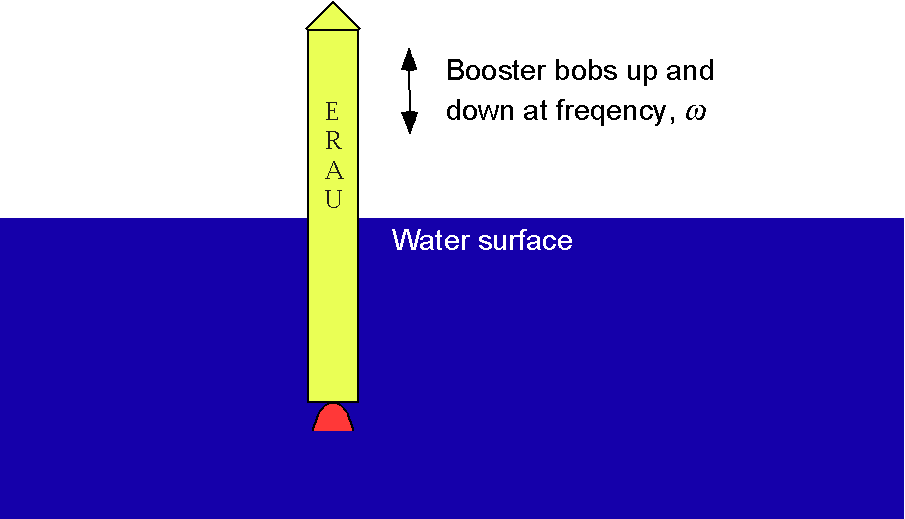
Using the information provided, the frequency of motion can be written in an explicit functional form as
![\[ \omega = \phi (D, \, m, \, \varrho, \, g) \]](https://eaglepubs.erau.edu/app/uploads/quicklatex/quicklatex.com-77e9e8c4b388b0d9d67f21e75cf1cccd_l3.svg "Rendered by QuickLaTeX.com")
where is some function to be determined, or in implicit form as
![\[ \psi (d, \, m, \, \varrho, \, g, \, \omega) = 0 \]](https://eaglepubs.erau.edu/app/uploads/quicklatex/quicklatex.com-95e39f9784815abafa9013049001bf7d_l3.svg "Rendered by QuickLaTeX.com")
where  is some other function. Therefore, , and so there are two products. The repeating variables must collectively include all the dimensions of mass
  , length
  , and time
  , so the best choice here is ,
  , and
, and  . Notice that if were to be chosen instead of as a repeating variable, then collectively, the repeating variables would not include time . So, the Buckingham method will fail in this case. The dependent variable, , cannot be used as a repeating variable. Therefore, the two products are
![\[ \Pi_1 = \phi_1(d, m, g, \omega) \]](https://eaglepubs.erau.edu/app/uploads/quicklatex/quicklatex.com-f21d4fc357b5512041a258ac52bb7526_l3.svg "Rendered by QuickLaTeX.com")
and
![\[ \Pi_2 = \phi_2(d, m, g, \varrho) \]](https://eaglepubs.erau.edu/app/uploads/quicklatex/quicklatex.com-bda8770e17b5f2792f1e637fd9b050c9_l3.svg "Rendered by QuickLaTeX.com")
where and are arbitrary functions. The dimensional matrix is
![\[ \begin{array}{l|r|r|r|r|r}\mbox{\small Base~unit} & d & m & g & \omega & \varrho \\ \hline\text{\small Mass, M} \quad & 0 & 1 & 0 & 0 & 1 \\\text{\small Length, L} \quad & 1 & 0 & 1 & 0 & -3 \\\text{\small Time, T} \quad & 0 & 0 & -2 & -1 & 0\end{array} \]](https://eaglepubs.erau.edu/app/uploads/quicklatex/quicklatex.com-6e0c6487d6747c2b5154dbc8e29f7f1f_l3.svg "Rendered by QuickLaTeX.com")
The first product is
![\[\small \Pi_{1} = (d)^{\alpha} (m)^{\beta} (g)^{\gamma} \omega \]](https://eaglepubs.erau.edu/app/uploads/quicklatex/quicklatex.com-0af56e1375a12436915747ada8c1eeb9_l3.svg "Rendered by QuickLaTeX.com")
where the values of the coefficients , , and must be obtained to make the equation dimensionally homogeneous and dimensionless. In terms of the dimensions of the parameters, then
![\[ \left[ \Pi_{1} \right] = \rm M^{0}L^{0}T^{0} = \left( \rm L \right)^{\alpha} \left( \rm M \right)^{\beta} \left( \rm L T^{-2} \right)^{\gamma} \left(\rm T^{-1}\right) \]](https://eaglepubs.erau.edu/app/uploads/quicklatex/quicklatex.com-fa7f5861b9a51e05ef2bb55421c0984a_l3.svg "Rendered by QuickLaTeX.com")
For to be dimensionless, then the powers or exponents of M, L, and T must add to zero, i.e., in this case
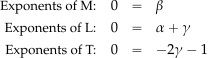
Therefore,  , , and , so the product is
![\[ \Pi_1 = (d)^{1/2} (m)^{0} (g)^{-1/2} \omega = \omega \sqrt{\frac{d}{g}} \]](https://eaglepubs.erau.edu/app/uploads/quicklatex/quicklatex.com-1b89f8d0c3c158842ecdabb31a6a0209_l3.svg "Rendered by QuickLaTeX.com")
which is a dimensionless pendular frequency.
For the second product then
![\[ \Pi_{2} = (d)^{\alpha} (m)^{\beta} (g)^{\gamma} \varrho \]](https://eaglepubs.erau.edu/app/uploads/quicklatex/quicklatex.com-9c8b1bd70a58566830cd6b753e5e13cc_l3.svg "Rendered by QuickLaTeX.com")
In terms of the dimensions, then
![\[ \left[ \Pi_{2} \right] = \rm M^{0}L^{0}T^{0} = \left(\rm L \right)^{\alpha} \left(\rm M \right)^{\beta} \left( L T^{-2} \right)^{\gamma} \left( \rm ML^{-3}\right) \]](https://eaglepubs.erau.edu/app/uploads/quicklatex/quicklatex.com-e20c035f556cc410176cbf7aff6417cc_l3.svg "Rendered by QuickLaTeX.com")
For to be dimensionless, then
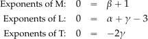
Therefore, = -1, = 0, and  , so the product is
![\[ \Pi_2 = (d)^{3} (m)^{-1} (g)^{0} \varrho = \frac{\varrho \, d^3}{m} \]](https://eaglepubs.erau.edu/app/uploads/quicklatex/quicklatex.com-a14454e9d8b6273b1f5a2f2220c90720_l3.svg "Rendered by QuickLaTeX.com")
which is a buoyancy similarity parameter, i.e., the ratio of the mass  (or weight
  ) of the water displaced to the mass (or weight
  ) of the rocket booster.
Finally, in dimensionless form, then
![\[ \Pi_{1} = \phi_3 (\Pi_2) \]](https://eaglepubs.erau.edu/app/uploads/quicklatex/quicklatex.com-e48139b991ff4c5634a25437bbf03af3_l3.svg "Rendered by QuickLaTeX.com")
or that
![\[ \omega \sqrt{\frac{d}{g}} = \phi_3 \left( \frac{\varrho \, d^3}{m}\right) \]](https://eaglepubs.erau.edu/app/uploads/quicklatex/quicklatex.com-5c356d89ac78085344aaa8219ec27fdc_l3.svg "Rendered by QuickLaTeX.com")
Check the final dimensions of the grouping to be sure it is dimensionless, i.e., it has dimensions of 1. So, in this case
![\[ \left[ \omega \sqrt{\frac{d}{g}} \right] = \rm T^{-1} \sqrt{\frac{L}{L T^{-2}}} = 1 \]](https://eaglepubs.erau.edu/app/uploads/quicklatex/quicklatex.com-6b820b95efbf26fcf25db0b5730374f9_l3.svg "Rendered by QuickLaTeX.com")
and
![\[ \left[ \frac{\varrho \, d^3}{m} \right] = \rm \frac{ M L^{-3} L^{3} }{M} = 1 \]](https://eaglepubs.erau.edu/app/uploads/quicklatex/quicklatex.com-a2e3327d3838fade3d7a3a21c05b44a7_l3.svg "Rendered by QuickLaTeX.com")
which confirms that the two groupings are dimensionless.
Worked Example #39 – Rollover wind speed for a trailer
The wind speed, , required to destabilize a trailer of mass and height , depends on the gravitational acceleration , the air density  , and the base width
  of the trailer. Take the wind speed as the dependent variable and the other parameters as independent variables. Determine the dimensionless grouping that involves air density and confirm that the grouping is dimensionless. Hints: 1. Choose , , and as the repeating variables. 2. Use only the Buckingham
  method and show all steps.
The wind speed, , required to destabilize a trailer can be expressed in functional form as
![\[ V = \phi \left( m, \, h, \, g, \, \varrho, \, b \right) \]](https://eaglepubs.erau.edu/app/uploads/quicklatex/quicklatex.com-5ca2f17cca240a27cdf03fe23861d2e8_l3.svg "Rendered by QuickLaTeX.com")
In implicit form, this relationship can also be expressed as
![\[ \psi \left( V, \, m, \, h, \, g, \, \varrho, \, b \right) = 0 \]](https://eaglepubs.erau.edu/app/uploads/quicklatex/quicklatex.com-b55db2a76f2fbdcac8d9018e6dbac84f_l3.svg "Rendered by QuickLaTeX.com")
Because we have parameters and three fundamental dimensions () , there will be  , so three groups. The dimensions of each parameter are
![\[ \begin{aligned} \left[ V \right] &= \rm L T^{-1} \\ \left[ m \right] &= \rm M\\ \left[ h \right] &= \rm L \\ \left[ g \right] &= \rm L T^{-2} \\ \left[ \varrho \right] &= \rm M L^{-3} \\ \left[ b \right] &= \rm L \end{aligned} \]](https://eaglepubs.erau.edu/app/uploads/quicklatex/quicklatex.com-503ebc5d60633490373c84abce4a8e9f_l3.svg "Rendered by QuickLaTeX.com")
The dimensional matrix is
![\[ \begin{array}{l|r|r|r|r|r|r} \mbox{\small Base~unit} & V & m & h & g & \varrho & b \\ \hline \mbox{\small Mass M:} & 0 & 1 & 0 & 0 & 1 & 0 \\ \mbox{\small Length L:} & 1 & 0 & 1 & 1 & -3 & 1 \\ \mbox{\small Time T:} & -1 & 0 & 0 & -2 & 0 & 0 \end{array} \]](https://eaglepubs.erau.edu/app/uploads/quicklatex/quicklatex.com-5c2a3d4e045cd630d4bba05730066b06_l3.svg "Rendered by QuickLaTeX.com")
According to the hint, , , and are to be used as the repeating variables. They are a valid choice because they include all three fundamental dimensions, M, L, and T. Therefore, the three dimensionless groups will be
![\[ \Pi_1 = \phi_1 (m, \, h, \, g, \, V), \quad \Pi_2 = \phi_2 (m, \, h, \, g, \, \varrho), \quad \Pi_3 = \phi_3 (m, \, h, \, g, \, b) \]](https://eaglepubs.erau.edu/app/uploads/quicklatex/quicklatex.com-7e228e6947d6aa737850f0a53229297d_l3.svg "Rendered by QuickLaTeX.com")
The first grouping, , will be
![\[ \Pi_1 = m^\alpha \, h^\beta \, g^\gamma \, V \]](https://eaglepubs.erau.edu/app/uploads/quicklatex/quicklatex.com-abd8bc64a4579a43ed60d91c2274fe0f_l3.svg "Rendered by QuickLaTeX.com")
Substituting the dimensions gives
![\[ \left[ \Pi_1 \right] = 1 = \rm \left( M \right)^{\alpha} \left( L \right)^{\beta} \left( L T^{-2} \right)^{\gamma} \left( L T^{-1} \right) \]](https://eaglepubs.erau.edu/app/uploads/quicklatex/quicklatex.com-701c4b79a8e545ac18703e7d625b0e4c_l3.svg "Rendered by QuickLaTeX.com")
Equating the exponents gives ,  , and
, and  . Solving for
  gives
gives  . Substituting into
  gives
gives  . Therefore, the first dimensionless group is
![\[ \Pi_1 = \frac{V}{\sqrt{g \, h}} \]](https://eaglepubs.erau.edu/app/uploads/quicklatex/quicklatex.com-b7d574985bb9f306e8117c4cc67cfcab_l3.svg "Rendered by QuickLaTeX.com")
This grouping is recognized as the Froude number, i.e.,
![\[ Fr = \frac{V}{\sqrt{g \, h}} \]](https://eaglepubs.erau.edu/app/uploads/quicklatex/quicklatex.com-f45de59983e521c2b05c18508a1197d9_l3.svg "Rendered by QuickLaTeX.com")
For , then
![\[ \Pi_2 = m^\alpha \, h^\beta \, g^\gamma \, \varrho \]](https://eaglepubs.erau.edu/app/uploads/quicklatex/quicklatex.com-6a1ff4778037e8cda6519711f29a5c40_l3.svg "Rendered by QuickLaTeX.com")
Substituting the dimensions gives
![\[ \left[ \Pi_2 \right] = 1 = \rm \left( M \right)^{\alpha} \left( L \right)^{\beta} \left( L T^{-2} \right)^{\gamma} \left( M L^{-3} \right) \]](https://eaglepubs.erau.edu/app/uploads/quicklatex/quicklatex.com-a80b9186f037644c0f0431fd365d37b9_l3.svg "Rendered by QuickLaTeX.com")
Equating the exponents gives  , so , and
  , and
, and  , so Substituting into
  gives
gives  . Therefore, the second dimensionless group is
![\[ \Pi_2 = \frac{\varrho \, h^3}{m} \]](https://eaglepubs.erau.edu/app/uploads/quicklatex/quicklatex.com-b06b1b14dafb00138a232e0dc368f3bf_l3.svg "Rendered by QuickLaTeX.com")
To confirm this interesting grouping, we can check its dimensions, i.e.,
![\[ \left[ \frac{\varrho \, h^3}{m} \right] = \frac{\left( M L^{-3} \right) \left( L^3 \right)}{M} = \frac{M L^{-3} L^3}{M} = \frac{M}{M} = 1 \]](https://eaglepubs.erau.edu/app/uploads/quicklatex/quicklatex.com-e7c7b19bddba9870eaa10c381d7dfe9e_l3.svg "Rendered by QuickLaTeX.com")
Therefore, because all three groups are dimensionless, the relationship must be of the form
![\[ Fr = \phi \left( \frac{\varrho \, h^3}{m}, \frac{b}{h} \right) \]](https://eaglepubs.erau.edu/app/uploads/quicklatex/quicklatex.com-882932d046afdb9d8b46c96cd47238a6_l3.svg "Rendered by QuickLaTeX.com")
Notice that the tip-over speed of a trailer depends on the Froude number, not just the wind speed, because it represents the balance between wind-induced inertia and gravitational restoring forces. The wind force acting on the trailer is proportional to the dynamic pressure, i.e.,
![\[ F_{\text{wind}} \quad \propto \quad \dfrac{1}{2} \varrho \, V^2 \, A, \quad A = h \, b \]](https://eaglepubs.erau.edu/app/uploads/quicklatex/quicklatex.com-da287b4bc80a53249f2a78b1e0c445fd_l3.svg "Rendered by QuickLaTeX.com")
This force creates a moment about the leeward wheel, i.e.,
![\[ M_{\text{wind}} \quad \propto \quad \dfrac{1}{2} \varrho \, V^2 \, A \, h \]](https://eaglepubs.erau.edu/app/uploads/quicklatex/quicklatex.com-2640f070cfb6da311cbfb73cd271395a_l3.svg "Rendered by QuickLaTeX.com")
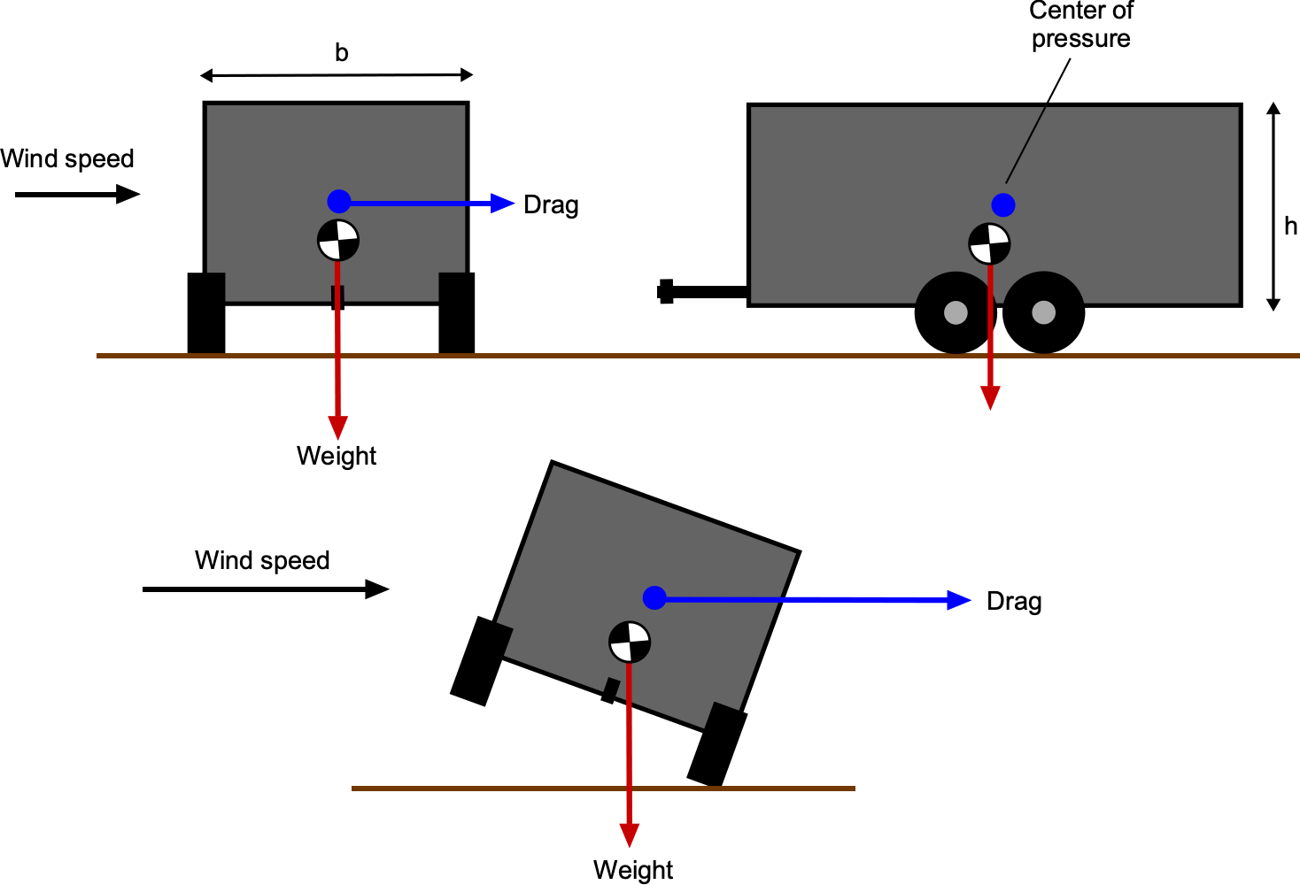
The restoring moment from gravity is
![\[ M_{\text{gravity}} = m \, g \, \frac{b}{2} \]](https://eaglepubs.erau.edu/app/uploads/quicklatex/quicklatex.com-c1e9a8f2dbedd416793a42d33f7d5f6a_l3.svg "Rendered by QuickLaTeX.com")
Tipping occurs when  , giving the critical wind speed as
![\[ V_{\rm crit} \geq \sqrt{\frac{m \, g \, b}{\varrho \, h^2 \, A}} \]](https://eaglepubs.erau.edu/app/uploads/quicklatex/quicklatex.com-400883e9e7a46fff8306e74de9a3819e_l3.svg "Rendered by QuickLaTeX.com")
Because the Froude number is defined as
it follows that
![\[ Fr \quad \propto \quad \sqrt{\frac{m \, b}{\varrho \, h^3}} \]](https://eaglepubs.erau.edu/app/uploads/quicklatex/quicklatex.com-fed1a7f45db5c57021f5e90cfa4d1e1c_l3.svg "Rendered by QuickLaTeX.com")
Therefore, the tip-over speed depends on because it determines whether the inertia in the wind dominates over gravitational stability.
Worked Example #40 – Dynamic similarity in the wind tunnel
The aerodynamic drag of a prototype race car is to be predicted at a speed of 60 mph to compare with a CFD solution. Engineers build a one-fourth-scale model of the car to test in a wind tunnel. The drag force is measured with a balance. Determine how fast the engineers should run the wind tunnel to achieve dynamic flow similarity between the wind tunnel model and the prototype car. The aerodynamic drag on the model in the wind tunnel is measured to be 36.5 lb when the wind tunnel is operated at a speed that ensures similarity with the prototype car. Estimate the drag force on the actual car. State any assumptions you may make and why. Assume all conditions are MSL ISA. Discuss any other issues that may affect the drag value measured on the wind tunnel model.

In the wind tunnel, we want to match the Reynolds numbers between the actual car and the model to get flow similarity. The Reynolds number for the actual car can be written as
and for the model
Therefore, we have that
if the flow conditions (e.g., temperature and pressure, hence its density and viscosity) are the same in the wind tunnel as those for the actual car.
The ratio  (i.e., one-fourth scale), so
![\[ V_2 = 4 V_1 = 240~\mbox{mph} \]](https://eaglepubs.erau.edu/app/uploads/quicklatex/quicklatex.com-737e867b19a80337f68c94ed1246cb61_l3.svg "Rendered by QuickLaTeX.com")
While much faster, this speed is still low enough that compressibility effects will be minor, so there is no need to worry about Mach number scaling.
The drag force on the actual car can be written as
where is a reference area on which the drag coefficient is based. It is reasonable to assume the drag coefficient on both the actual car and the model is the same, which is typical of bluff bodies like cars. The drag force on the model can be written as
where the ratio  , i.e., lengths scale linearly but areas scale by the square. Therefore, we can write
![\[ \frac{D_2}{D_1} = \left( \frac{V_2}{V_1} \right)^2 \ \frac{A_2}{A_1} = \left( \frac{4V_1}{V_1} \right)^2 \ \frac{1}{16} = 1 \]](https://eaglepubs.erau.edu/app/uploads/quicklatex/quicklatex.com-b3f0ea0cb3786de9e62e61bff2fc4f52_l3.svg "Rendered by QuickLaTeX.com")
We are told that  is 36.5 lb at the conditions of matching Reynolds number, so the drag on the actual car will be
  lb, i.e., exactly the same as in the wind tunnel!
This is an interesting and quite useful outcome that follows from the scaling relationships. The force on a body of a particular shape at a given Reynolds number is the same regardless of the combination of size and speed used to produce that given Reynolds number. Of course, the flow conditions (e.g., temperature and pressure, hence density and viscosity) must also be the same.
Worked Example #41 – Are the flows dynamically similar?
Consider the flow about two geometrically similar airfoils, with one having four times the chord of the other airfoil, as shown in the figure below. The freestream parameters are very different, such that:
![\[ V_2 = 2 V_1, \quad \varrho_2 = \frac{ \varrho_1 }{4}, \quad \mbox{~and~} \quad T_2 = 4 T_1 \]](https://eaglepubs.erau.edu/app/uploads/quicklatex/quicklatex.com-87302a8f62d9a71029125c53729106f3_l3.svg "Rendered by QuickLaTeX.com")
Are the flows dynamically similar? This outcome is certainly not obvious!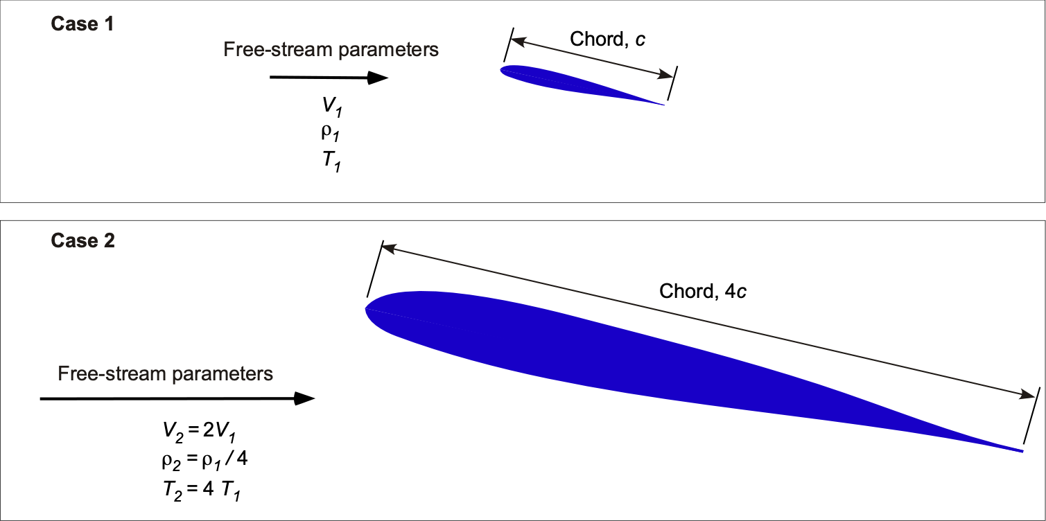
To find out, it is to be determined if the flow similarity parameters are the same for both flows, i.e., specifically to determine if
 and
and  . For the first flow, then
![\[ Re_{1} = \frac{\varrho_{1} V_{1} c}{\mu_{1}} \]](https://eaglepubs.erau.edu/app/uploads/quicklatex/quicklatex.com-4ee6757cb2ee931fc8b474065c41ad1b_l3.svg "Rendered by QuickLaTeX.com")
and for the second flow, then
![\[ Re_{2} = \frac{\varrho_{2} V_{2} 4c}{\mu_{2}} = \frac{\varrho_{1}}{4} \frac{2V_{1}4c}{\mu_{2}} = \frac{2\varrho_{1}V_{1}}{\mu_{2}} \]](https://eaglepubs.erau.edu/app/uploads/quicklatex/quicklatex.com-2f8ce34d3f3b548fadce152b5c40b18e_l3.svg "Rendered by QuickLaTeX.com")
Therefore,
![\[ \frac{Re_{1}}{Re_{2}} = \frac{\varrho_{1}V_{1}c}{\mu_{1}} \frac{\mu_{2}}{2\varrho_{1}V_{1}c} = \frac{\mu_{2}}{2\mu_{1}} \]](https://eaglepubs.erau.edu/app/uploads/quicklatex/quicklatex.com-41587b909c5760a9fa5ee151e9722230_l3.svg "Rendered by QuickLaTeX.com")
For a gas then  is a good approximation, so that
![\[ \frac{\mu_{1}}{\mu_{2}} = \frac{\sqrt{T_{1}}}{\sqrt{T_{2}}} \]](https://eaglepubs.erau.edu/app/uploads/quicklatex/quicklatex.com-47bb6da2342c446a67206639a003bc5e_l3.svg "Rendered by QuickLaTeX.com")
Therefore,
![\[ \frac{Re_{1}}{Re_{2}} = \frac{\mu_{2}}{2\mu_{1}} = \frac{\sqrt{T_{2}}}{2\sqrt{T_{1}}}= \frac{\sqrt{4T_{1}}}{2\sqrt{T_{1}}} = \frac{2\sqrt{T_{1}}}{2\sqrt{T_{1}}} = 1 \]](https://eaglepubs.erau.edu/app/uploads/quicklatex/quicklatex.com-9995efa2e57ad6ffee982503a86fe7b2_l3.svg "Rendered by QuickLaTeX.com")
and so
![\[ Re_{1} = Re_{2} \]](https://eaglepubs.erau.edu/app/uploads/quicklatex/quicklatex.com-380fd40041d6cb4c768f1cff03989c17_l3.svg "Rendered by QuickLaTeX.com")
So, the Reynolds numbers for both flows are equal.
The Mach numbers for the two flows are given by
![\[ M_{1} = \frac{V_{1}}{a_{1}} \mbox{ \quad and \quad } M_{2} = \frac{V_{2}}{a_{2}} = \frac{2V_{1}}{a_{2}} \]](https://eaglepubs.erau.edu/app/uploads/quicklatex/quicklatex.com-2ee6d9be978af81cf884de5202c824fd_l3.svg "Rendered by QuickLaTeX.com")
so
![\[ \frac{M_{1}}{M_{2}} = \frac{a_{2}}{2a_{1}} \]](https://eaglepubs.erau.edu/app/uploads/quicklatex/quicklatex.com-f9e10a31930a2d772fc0c44f34bb1005_l3.svg "Rendered by QuickLaTeX.com")
It is also known that  , so
, so
![\[ \frac{a_{1}}{a_{2}} = \frac{\sqrt{T_{1}}}{\sqrt{T_{2}}} \]](https://eaglepubs.erau.edu/app/uploads/quicklatex/quicklatex.com-aa3d71f224dc31b98c683da1af30c6f1_l3.svg "Rendered by QuickLaTeX.com")
and then
![\[ \frac{M_{1}}{M_{2}} = \frac{a_{2}}{2a_{1}} = \frac{\sqrt{T_2}}{2\sqrt{T_2}}=\frac{\sqrt{4T_1}} {2\sqrt{T_2}} = \frac{2\sqrt{T_1}}{2\sqrt{T_1}} = 1 \]](https://eaglepubs.erau.edu/app/uploads/quicklatex/quicklatex.com-928af589e1f96a5b3811f7dc253b44ac_l3.svg "Rendered by QuickLaTeX.com")
giving
![\[ M_{1}= M_{2} \]](https://eaglepubs.erau.edu/app/uploads/quicklatex/quicklatex.com-ad2e4b91363cc28630ef6702317ea320_l3.svg "Rendered by QuickLaTeX.com")
Therefore, because the two similarity parameters (Reynolds number and Mach number) are the same for both flows, the two flows will be dynamically similar. Dynamic similarity is an essential concept for engineers and scientists because it allows them to extrapolate results from one system to another and make predictions about physical behaviors without testing full-scale systems, which can be expensive and impractical.
Worked Example #41 – Dynamic similarity in the wind tunnel
A  -scale model of a small light-sport airplane is tested in a wind tunnel, and the lift force is measured to be
  lb at an airspeed of
  ft/s in standard air conditions at sea level. Assuming Reynolds-number effects are negligible, estimate the lift force on the full-scale airplane when flying at
  ft/s at the same angle of attack and under the same atmospheric conditions.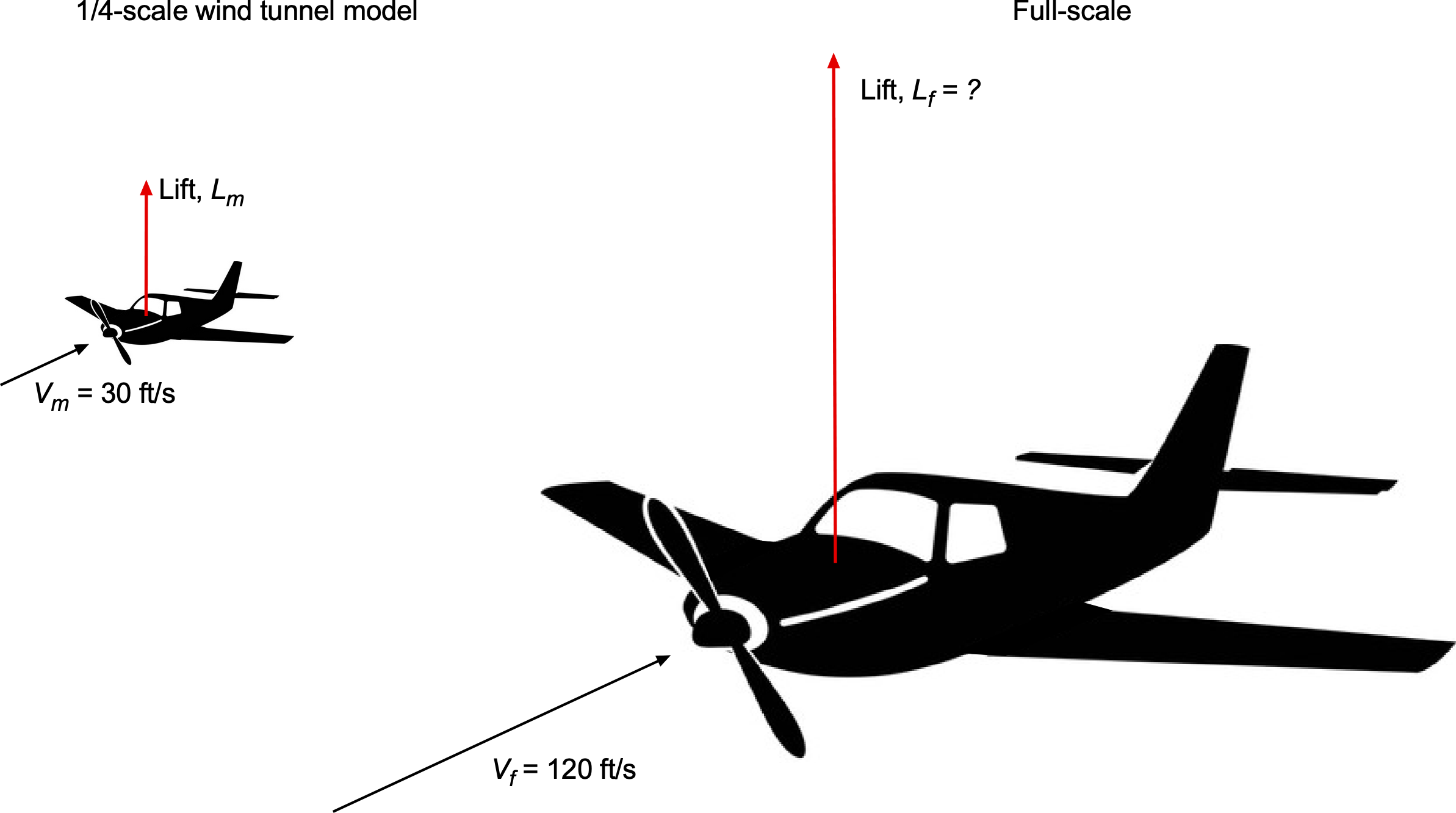
Because the lift is given by
![\[ L = \dfrac{1}{2} \varrho V^2 S C_L \]](https://eaglepubs.erau.edu/app/uploads/quicklatex/quicklatex.com-941b0b429bc723a6c2659e2dcb945b06_l3.svg "Rendered by QuickLaTeX.com")
then
![\[ \frac{L_f}{L_m} = \left( \frac{V_f}{V_m} \right)^2 \, \left( \frac{S_f}{S_m} \right) \]](https://eaglepubs.erau.edu/app/uploads/quicklatex/quicklatex.com-acf2d0f2e208192cefece88dbb8c5b39_l3.svg "Rendered by QuickLaTeX.com")
where  is the lift on the model,
  is the lift on the full-scale airplane,
  is the airspeed of the model in the wind tunnel, and is the airspeed of the full-scale airplane.
This is a -scale model, so the wing area ratio is
![\[ \frac{S_f}{S_m} = 4^2 = 16 \]](https://eaglepubs.erau.edu/app/uploads/quicklatex/quicklatex.com-09ae9d34228691732dc96b20a7695ca9_l3.svg "Rendered by QuickLaTeX.com")
The ratios of the lift forces at the same lift coefficient (or angle of attack) will then be
![\[ \frac{L_f}{10.5} = \left(\frac{120}{30}\right)^2 \times 16 = (4)^2 \times 16 = 256 \]](https://eaglepubs.erau.edu/app/uploads/quicklatex/quicklatex.com-e3b3f7ab4097249a6f665c90fe7f5e86_l3.svg "Rendered by QuickLaTeX.com")
Therefore,
![\[ L_f = 10.5 \times 256 = 2,688 \text{ lb} \]](https://eaglepubs.erau.edu/app/uploads/quicklatex/quicklatex.com-850395e5c9e511364b99b40d074b8a7d_l3.svg "Rendered by QuickLaTeX.com")