26 Bluff Body Flows
Introduction
Aerospace engineers are more often than not interested in the aerodynamics of smooth, slender, streamlined shapes that gradually taper to a sharp point at their trailing edges, e.g., airfoils and wings. However, non-streamlined or unstreamlined shapes with blunt front and/or rear faces, called bluff bodies (sometimes referred to as blunt bodies), are also encountered in many engineering applications. While the drag force on a body shape comprises the effects of the two primary contributors, skin friction drag and pressure drag, the total drag on bluff bodies is typically dominated by the pressure drag component. This outcome results from the effects of the large low-pressure zone formed in the wake behind the body, as illustrated in the diagram below.
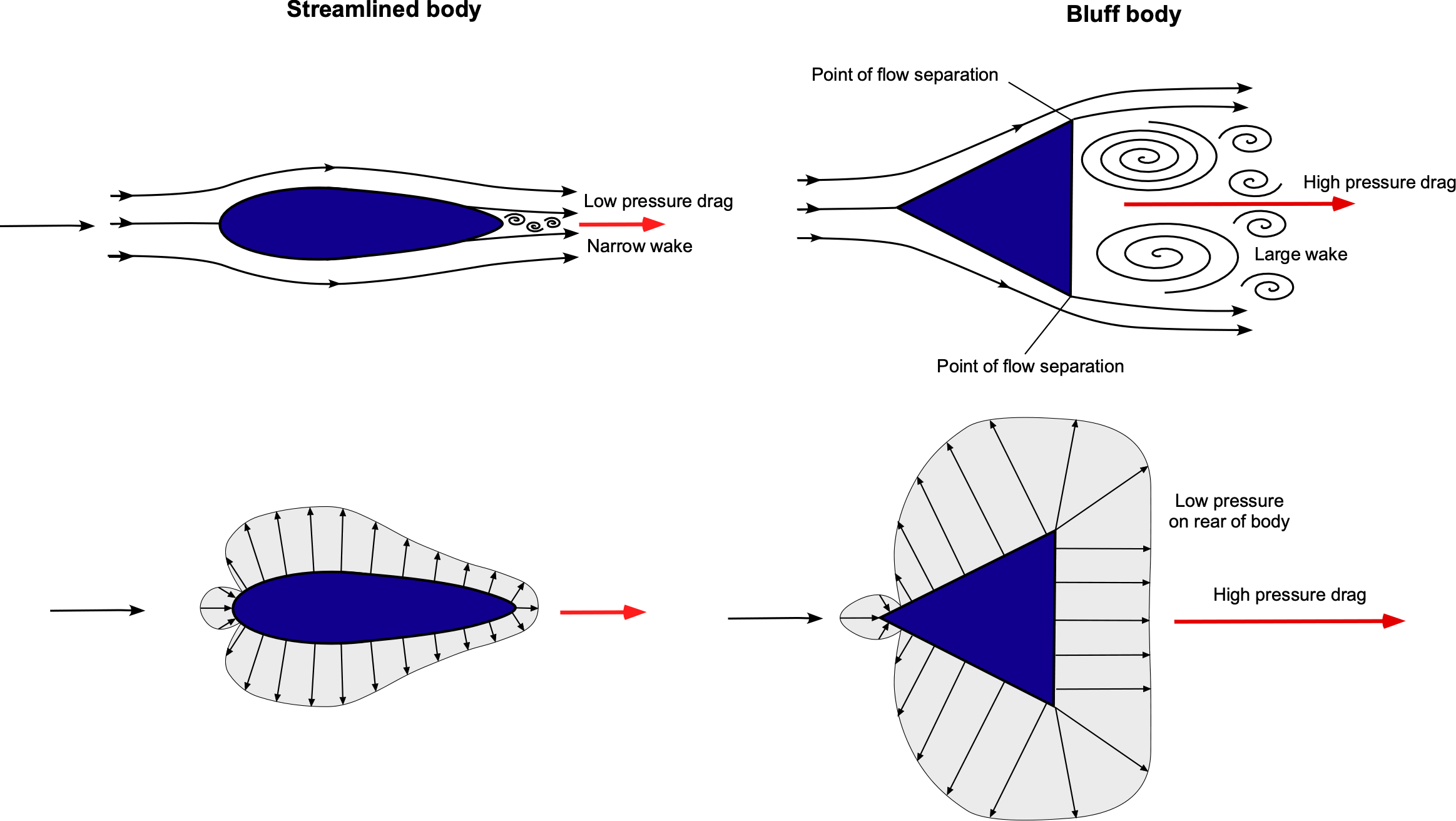
Understanding bluff body aerodynamics is essential because of its wide-ranging applications in various engineering fields. Studying how non-streamlined objects interact with airflows helps design more efficient structures and vehicles. For instance, understanding unsteady wind loads on bluff body shapes, such as buildings and bridges, ensures aeroelastic stability and prevents failures. Optimizing vehicle shapes reduces drag, improves fuel efficiency, and leads to better performance. The aerodynamics of bluff bodies also comes into consideration in many sports, including golf, tennis, and baseball. For example, the dimples on a golf ball create turbulent flow, which reduces drag and allows the ball to travel further. In tennis, the spin imparted on the ball affects its trajectory and speed. Similarly, in baseball, the stitching on the ball and the way it is thrown, such as with spin, create varying aerodynamic effects based on the players’ skill.
Learning Objectives
- Distinguish the fundamental differences between the flows of streamlined versus bluff bodies.
- Understand the use of reference areas in defining bluff body drag coefficients and the concept of equivalent drag area.
- Appreciate why the drag of bluff bodies with smooth surfaces, such as circular cylinders and spheres, shows sensitivities to Reynolds number variations.
- Become familiar with the Magnus effect on spinning cylinders and spheres.
Drag Coefficients
For bluff bodies, the interest is usually in the drag on that body, mainly because experiments have found that drag is the dominant force. This observation, however, does not imply that bluff bodies cannot produce lift because many do. Nevertheless, examining only the drag characteristics of such bodies is convenient initially. Furthermore, bluff bodies may also produce pitching moments, which are sometimes necessary to know for certain types of engineering work, such as determining torsional loads.
Recall that the two-dimensional drag coefficient is
(1) 
where  is the drag per unit span, and
  is a characteristic length, e.g., for a circular cylinder,
  , where
  is its diameter.
In most cases, the drag coefficients for two-dimensional bluff bodies are presented in terms of per length,  , so the drag coefficient is defined as
(2) 
where the product  is equivalent to an area. In general, for a three-dimensional object, the drag coefficient is defined as
(3) 
where  is defined as the reference area, usually the projected frontal area. Using a sphere of diameter as an example, its projected area is
  . Likewise, a cube with side length will have a reference area of
However, caution must be exercised when defining drag coefficients for three-dimensional bodies, as the drag coefficient always depends on the definition of the body’s reference area, which may not be unique. For example, on the one hand, for specific bodies of revolution, the volumetric drag coefficient is used by convention, in which the reference area is the square of the cube root of the volume. On the other hand, in hydrodynamics, the analysis of submerged streamlined bodies uses the wetted surface area as the reference area. Therefore, to consistently use and compare drag coefficients, adopting the convention used in the particular field of application is imperative.
To avoid ambiguity in the definitions of drag coefficients for different body shapes, drag coefficients per se are not always used. Instead, the equivalent drag area is used, given the symbol  . The equivalent drag area is defined as
(4) 
where would be measured in units of area.
The advantage of using equivalent drag areas is that there is no ambiguity in defining a reference area. This approach is often used when estimating the drag of complex shapes composed of many simpler shapes, such as the drag of an entire airplane. In such a case, the equivalent drag area of the complex shape is obtained by a drag synthesis of the equivalent drag areas of  simple shapes, i.e.,
(5) 
However, it would be incorrect to write
(6) 
because the reference areas on which each value of  is based could be different, and generally will be. To take into account component interference, i.e., to make some allowance for flow interference effects between the different components, then
(7) 
where  and often
  will be used for aircraft drag synthesis without any other information, i.e., a 20% drag penalty from component interference effects.
Drag Coefficients of Simple Shapes
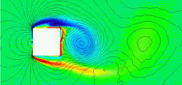
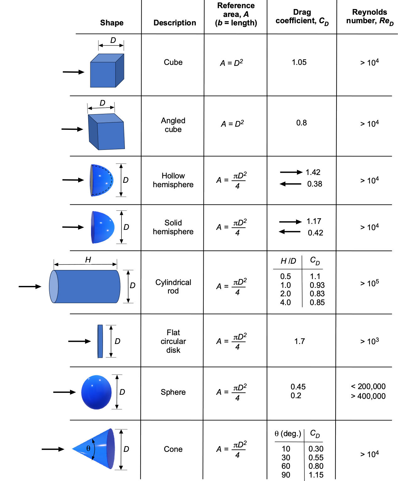
There are many bluff body shapes for which the drag (or drag coefficient) must be known for engineering purposes. However, in practice, far fewer such shapes are encountered, most of which have been well-studied, and the drag coefficients have been measured in wind tunnels. Furthermore, flows around bluff bodies are often unsteady and can produce various types of vortex shedding, as shown in the animation below. Therefore, the measurement or computation of drag is usually made over a relatively long period, known as an ensemble time average.
Drag coefficients for standard two-dimensional and three-dimensional bluff body shapes are published in numerous sources and serve as a valuable resource for engineers. These shapes can be further categorized into two primary sub-classes of bluff bodies:
- Those with sharp, angular shapes tend to have fixed points of flow separation and drag coefficients that are insensitive to the Reynolds number.
- Those with smooth contours will have variable flow separation points and can exhibit some sensitivity to the Reynolds number.
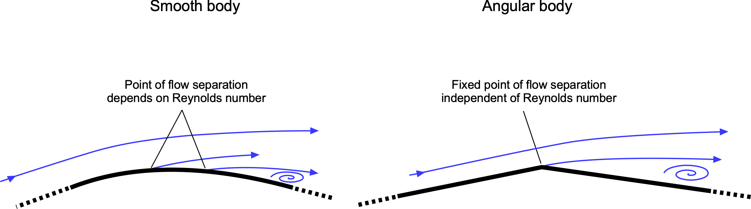
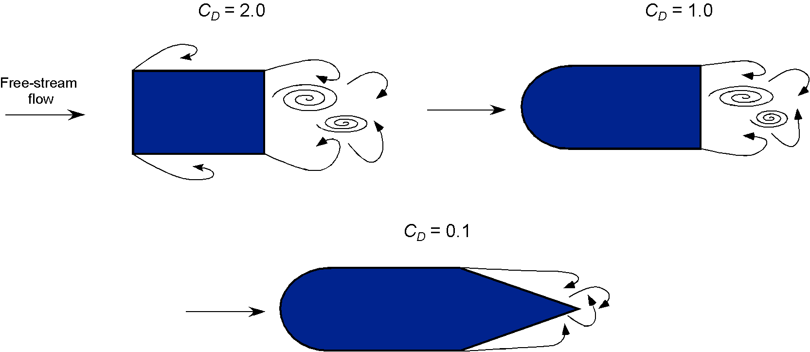
Of course, there is always the possibility that some bluff body shapes combine smooth contours and sharp edges. In this case, determining the drag coefficient and the effects of the Reynolds number may require specific measurements in the wind tunnel to establish the drag coefficients. Values for some common bluff-body shapes are shown in the tables below.
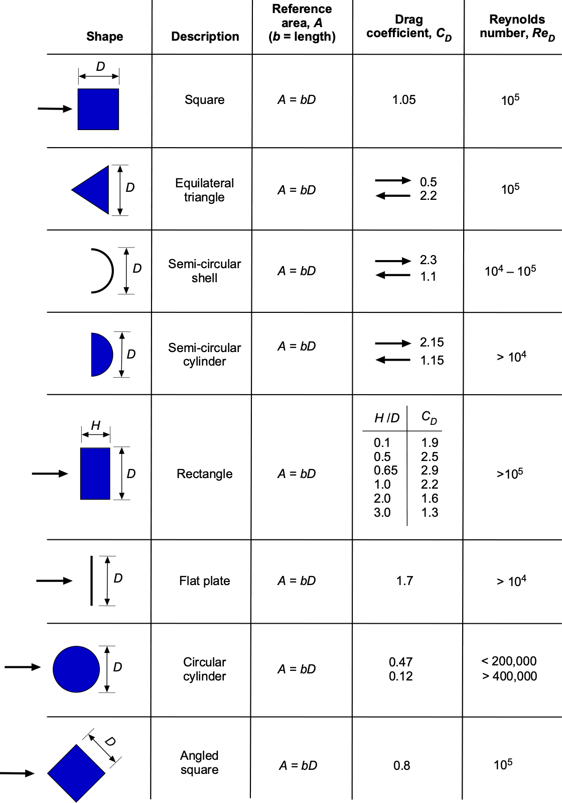
For example, a sphere or a cylinder is smooth, whereas a cube is angular. The flows about smooth bluff bodies or those with rounded corners generally exhibit some sensitivity to the Reynolds number, and their drag coefficients vary as a consequence, as shown in the tables. In contrast, angular shapes exhibit little to no variation with changes in the Reynolds number, at least after reaching a minimum threshold.
Check Your Understanding #1 – Calculating the drag on a bluff body
What will be the drag on a solid hemisphere with a frontal area of 0.26 m2 and a flow speed of 100 m/s? Hint: The drag will depend on which side of the hemisphere points into the wind.
Show solution/hide solution.
The drag force on the hemisphere is given by
![\[ D = \frac{1}{2} \varrho V ^2 \, C_D \, A_{\rm ref} \]](https://eaglepubs.erau.edu/app/uploads/quicklatex/quicklatex.com-0acba4c2206240b24f0b0904e1f1c527_l3.svg "Rendered by QuickLaTeX.com")
where  m2 and
  m/s, and if MSL ISA conditions are assumed then
  kg/m3. Looking up the value of a solid hemisphere’s drag coefficient in the table above, it can be seen that the value depends on whether the smooth side or the flat side faces the relative wind. In the former case,
  , and in the latter case,
  . Inserting the values for the smooth side facing the flow gives
![\[ D = \frac{1}{2} \varrho V ^2 \, C_D \, A_{\rm ref} = 0.5 \times 1.225 \times 100.0^2 \times 0.42 \times 0.26 = 668.9 \mbox{ N} \]](https://eaglepubs.erau.edu/app/uploads/quicklatex/quicklatex.com-a2e4292ed4f57b002da8d61b1622bfdd_l3.svg "Rendered by QuickLaTeX.com")
And for the flat side facing, the flow gives
![\[ D = \frac{1}{2} \varrho V ^2 \, C_D \, A_{\rm ref} = 0.5 \times 1.225 \times 100.0^2 \times 1.17 \times 0.26 = 1,863.2 \mbox{ N} \]](https://eaglepubs.erau.edu/app/uploads/quicklatex/quicklatex.com-5a9b5cdfa4a2e6fc7789bb04961805f4_l3.svg "Rendered by QuickLaTeX.com")
Flow Patterns Around a Circular Cylinder
A classic example of a well-studied two-dimensional bluff body flow is that of a circular cylinder, for which the flow readily separates near its maximum thickness or just downstream; representative examples are shown below. A wake is produced downstream of the cylinder, which usually contains turbulence and various sizes of vortical eddies. As might be expected for a smooth body, the flow about the cylinder and the resulting wake structure and drag are sensitive to variations in Reynolds number, which in this case is defined based on the diameter of the cylinder, .
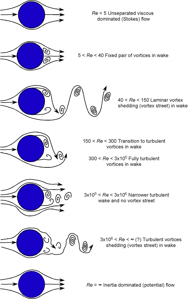
At very low Reynolds numbers, near unity, known as a “creeping flow” or Stokes flow, the behavior of the flow is significantly influenced by viscosity effects rather than inertia. At slightly higher Reynolds numbers but for  , a stable pair of symmetric vortices is formed in the wake of the cylinder; the flow is mainly steady, but a high drag coefficient is produced.
As the Reynolds number is further increased, the drag coefficient decreases to a point. The wake vortices move further downstream of the body in the form of alternative vortex shedding, producing two rows of counter-spinning vortices called a Von Kármán vortex street. This is an unsteady flow, creating an unsteady drag on the cylinder. However, no time-averaged unsteady lift is produced because of the strong asymmetry in the flow with respect to the flow direction. Interestingly, this latter type of periodically alternating flow also creates a periodic pressure field that manifests as a sound or noise, known as an Aeolian tone (after Aeolus, the Greek god of the wind). This effect is the source of the buzzing or “singing” sound sometimes heard when the wind blows over high-tension power wires.
As the Reynolds number increases, the periodic flow obtained about the cylinder at the lower Reynolds numbers becomes highly aperiodic, but still with the alternate shedding of vortices. Here, the flow in the wake is more turbulent. However, the boundary layer, which is of the turbulent kind, separates further down the surface, producing a narrower wake. Because the downstream wake is narrower, there is a smaller region of lower pressure on the downstream side, thereby giving lower drag.
As the Reynolds number increases, inertia effects begin to dominate over viscous effects. As a result, the flow becomes attached everywhere with a much smaller wake downstream of the cylinder, i.e., it starts to approach an inviscid flow. Because the flow is symmetric both upstream and downstream, the cylinder has no lift or drag force. This outcome is known as d’Alembert’s Paradox, after the mathematician Jean le Rond d’Alembert, who first addressed this problem by concluding that his theory for the flow did not align with experiments conducted on cylinders in a wind tunnel. The reason was that d’Alembert did not consider the action of viscosity in his solution, i.e., he considered only an inviscid flow. However, as shown in the images above, this flow type does not occur naturally because a real fluid is always viscous to some degree, and the Reynolds number is finite.
Drag of Circular Cylinders & Spheres
The corresponding drag coefficient on a circular cylinder as a function of the Reynolds number is shown in the figure below. Note that the results are for a smooth cylinder, and the effects of surface roughness alter the quantitative relationships. The drag coefficient for a sphere is also shown for reference. The drag reduces quickly with increasing Reynolds number  (note the logarithmic scales) until reaches approximately
  , after which the drag remains nominally constant. This outcome arises because the point of flow separation (laminar boundary layer separation) is delayed to a greater downstream distance, eventually separating close to the points of maximum thickness.
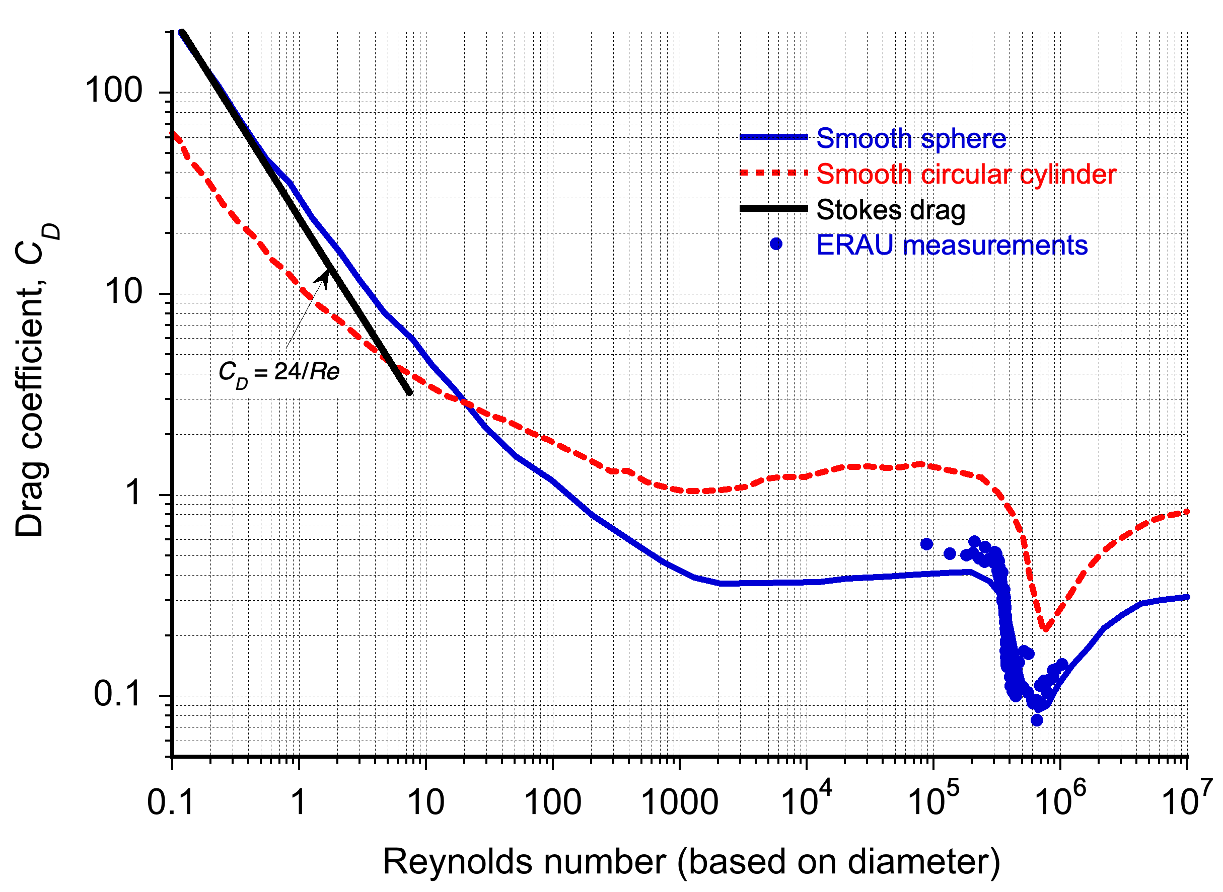
With further increases in , it will be apparent that there is a critical value of where the drag suddenly decreases by almost an order of magnitude. This condition, called the critical Reynolds number, corresponds to the reattachment of the previously separated laminar boundary layer as a turbulent boundary layer, which finally separates at a further downstream distance on the rear part of the cylinder. The critical Reynolds number for a cylinder is about = 2 x 10⁵. The narrower wake subsequently produces a reduction in pressure drag and overall drag. However, notice that with further increases in , the drag increases again because of the increasingly higher surface shear stresses (i.e., skin friction) produced by the turbulent boundary layer as the flow speed and Reynolds number increase.
The aerodynamic behavior of a sphere is qualitatively similar to that of a circular cylinder, as shown below. Again, there is a sudden drop in drag as the Reynolds number reaches a critical value because of the transition from laminar flow separation to turbulent separation. However, in this case, the surface roughness effects are of some interest, which can cause the drag reduction on the sphere to occur at a lower value of the critical Reynolds number.
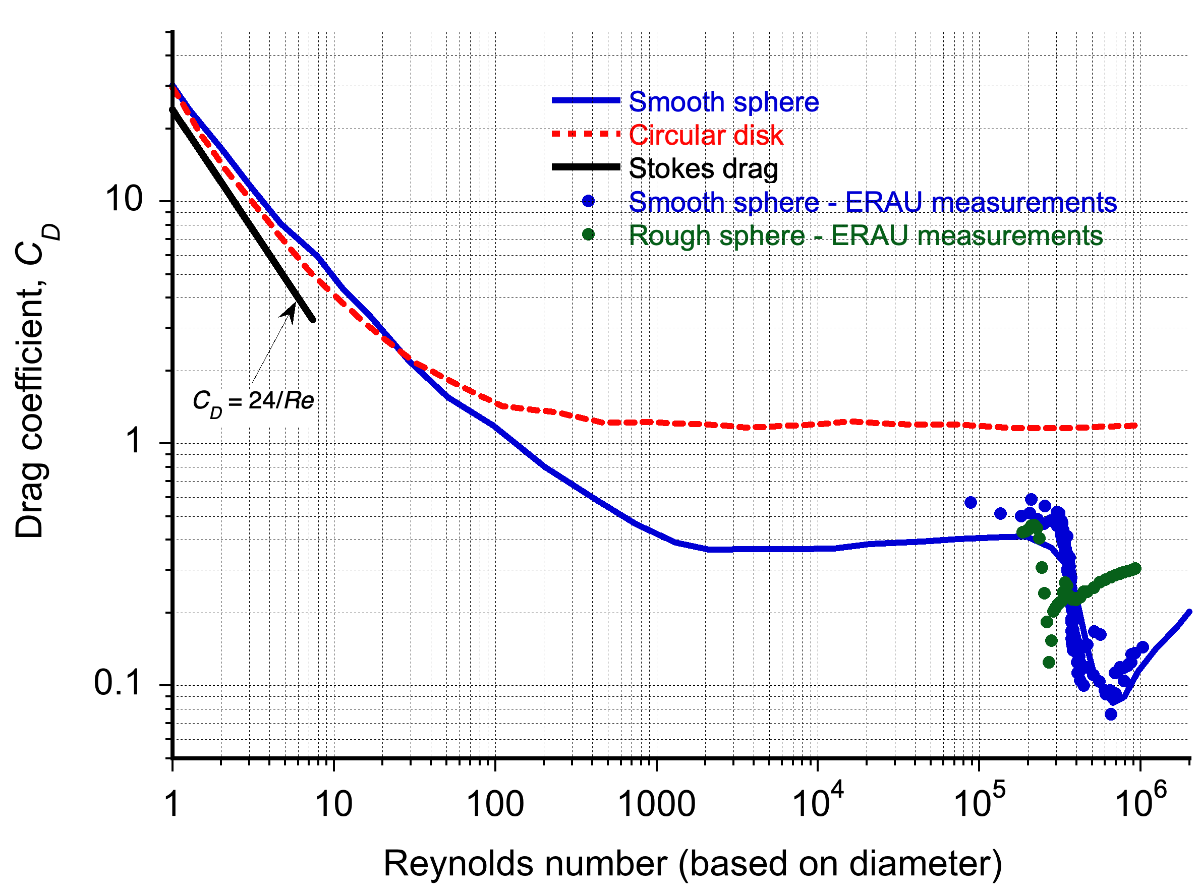
This latter behavior is illustrated below using flow visualization, where the roughness causes a significant reduction in the width and extent of the downstream wake. It explains the reduction in drag, i.e., the roughness manifests as an increase in the effective value of the Reynolds number. The surface roughness causes the laminar boundary layer on the upstream side of the sphere to transition immediately into a turbulent boundary layer, which can remain attached to the sphere’s surface much longer than a laminar boundary layer. The consequence of this behavior is the creation of a narrower low-pressure wake, resulting in lower drag on the sphere.
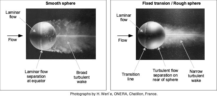
 , and the same sphere at the same Reynolds number with surface roughness (right).
Check Your Understanding #2 – Drag coefficient of a circular cylinder
Consider the airflow past a circular cylinder with a diameter, , of 0.4 meters. The freestream velocity,  , is 50 m/s. The properties of air at standard conditions are as follows:
  = 1.225 kg/m
 and
and  = 1.7894 x 10
 kg m
kg m s.
s.
- Determine the Reynolds number for this flow.
- Classify the flow regime around the cylinder as either laminar or turbulent.
- Determine the drag coefficient,
 , for the cylinder.
Show solution/hide solution.
- The Reynolds number is given by
![\[ Re = \frac{\varrho_{\infty} \, V_{\infty} \, d}{\mu_{\infty}} \]](https://eaglepubs.erau.edu/app/uploads/quicklatex/quicklatex.com-d25fc488bd1a381f0cece127efb27683_l3.svg "Rendered by QuickLaTeX.com")
Inserting the values gives
![\[ Re = \frac{1.225 \times 50.0 \times 0.4}{1.7894 \times 10^{-5} } = 1.369 \times 10^6 \]](https://eaglepubs.erau.edu/app/uploads/quicklatex/quicklatex.com-0e2a0e56efbb79354c03e4288680382a_l3.svg "Rendered by QuickLaTeX.com")
- The flow regime can be determined based on the Reynolds number. The critical Reynolds number for the transition from laminar to turbulent flow typically occurs at about 2 x 10
 for flow around a circular cylinder. In this case, the Reynolds number is well above this threshold, and the flow regime around the cylinder is turbulent.
 - The drag coefficient, , for a circular cylinder in turbulent flow can be estimated from the chart, which yields an approximate value of 0.12.
Why Do Golf Balls Have Dimples?
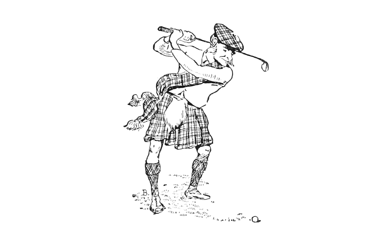
Ever wonder why a golf ball has dimples? Did you know that in the earliest days of golf, in the windy, cold links of Scotland, kilted golfers[1] made a remarkable discovery? They found that old, worn, and rough balls traveled further than new ones. This discovery was not just an observation; it had a significant impact on the game’s outcomes. Golfers[2]using these rough balls gained a golfer a considerable competitive edge, requiring many fewer strokes from the tee to the hole.
Unsurprisingly, the unique behavior of these rough spheres caught the attention of scientists, who began studying their aerodynamics in wind tunnels. These experiments revealed that rough spheres could have less aerodynamic drag than their smooth counterparts, as shown in the figure below. This discovery also led to the realization that standardizing golf balls was necessary to ensure a fair playing field for all golfers.
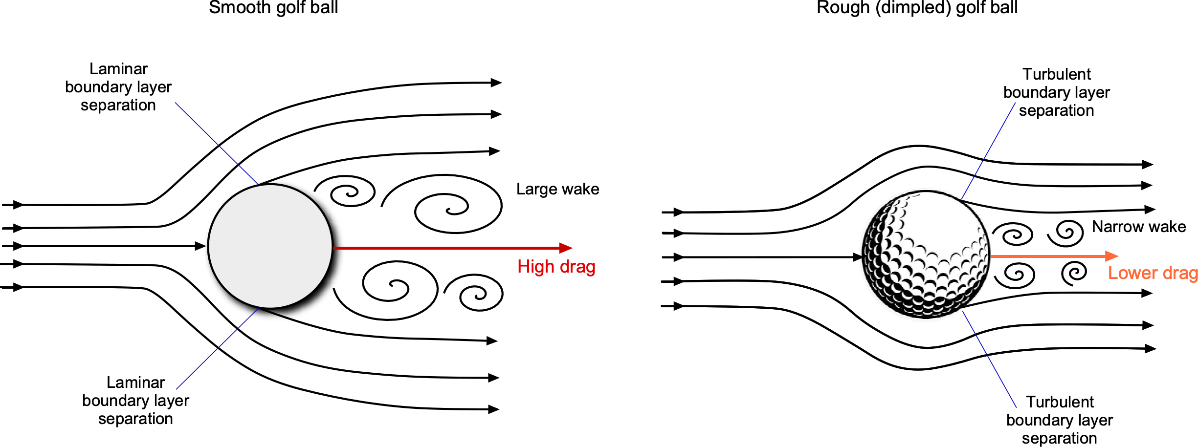
A modern golf ball is a machine-dimpled sphere, and the dimples act as surface roughness to deliberately change its aerodynamics. The dimples, a standardized form of roughness, cause the boundary layer on the upstream side of the ball to transition from laminar to turbulent, delaying flow separation and thereby reducing its drag. At the Reynolds numbers corresponding to the ball’s flight, which is about , the flow on a smooth ball would usually be laminar, and the flow would easily separate near the equator and cause higher pressure drag, as shown in the figure below.
However, a turbulent boundary layer, created using surface roughness, will remain attached to the ball’s surface much longer than a laminar boundary layer before it separates. This behavior creates a narrower low-pressure wake and less pressure drag. Interestingly, creating turbulence reduces drag, i.e., the dimples serve as a form of flow control. However, do not expect dimples to work on streamlined bodies, such as those of wings. The objective here is to keep the flow as smooth (laminar) for as long as possible, thereby reducing skin friction drag, which is the dominant drag source at low angles of attack. The addition of dimples can only serve to increase drag on a streamlined body. The upshot of less drag is that a golfer can hit the ball further.
This distance can be calculated using the laws of physics, specifically those related to ballistics and aerodynamics. One approximation for the range of the ball is given by
(8) 
where  is the initial velocity of the ball,
  is the initial hit trajectory angle of the ball (
 for maximum range),
  is the projected frontal area of the ball,
  is the mass of the ball,
  is the air density, and is the Reynolds number dependent drag coefficient based on ball diameter.
Notice that the range,  , is linearly dependent on the drag coefficient. Halving the drag will double the range, all other factors being equal. Does anyone want to try out the theory?
Check Your Understanding #3 – Reynolds number of a golf ball
What is a golf ball’s flight Reynolds number? What is the ball’s drag coefficient under the conditions of flight? Why is this important regarding the flight distance of a golf ball?
To answer this question, the issues to address are:
- What is the diameter of a golf ball?
- How fast does a golf ball travel?
Show solution/hide solution.
A little research will reveal that, according to golf rules, a golf ball’s diameter must be at least 1.68 inches (42.67 mm). Additionally, an amateur golfer typically hits a ball at an average speed of 135 mph (217.4 kph) with a driver club. However, those speeds can vary significantly with a golfer’s skill level and may range from a low of 110 mph (177 kph) to as high as 160 mph (257.5 kph) for a professional golfer. Therefore, the Reynolds number of a golf ball can only be established within certain bounds.
The Reynolds number of the golf ball based on its diameter is
![\[ Re = \frac{\varrho \, V d}{\mu} \]](https://eaglepubs.erau.edu/app/uploads/quicklatex/quicklatex.com-0c6c1902f870a8a47770ec56a7f2df30_l3.svg "Rendered by QuickLaTeX.com")
where and  can be assumed to take MSL ISA values, i.e., in SI units, then = 1.225 kg/m3 and = 1.48 x 10⁻⁵ kg m-1 s-1. Inserting the values using 257.5 kph or 71.53 m/s gives
![\[ Re = \frac{\varrho \, V d}{\mu} = \frac{1.225 \times 71.53 \times 0.04267}{1.48 \times 10^{-5}} = 2.13 \times 10^5 \]](https://eaglepubs.erau.edu/app/uploads/quicklatex/quicklatex.com-82c837a0f165cb85f1bdd835c62112cb_l3.svg "Rendered by QuickLaTeX.com")
and for 217.4 kph or 60.39 m/s gives
![\[ Re = \frac{\varrho \, V d}{\mu} = \frac{1.225 \times 60.39 \times 0.04267}{1.48 \times 10^{-5}} = 2.53 \times 10^5 \]](https://eaglepubs.erau.edu/app/uploads/quicklatex/quicklatex.com-e2ae9d69e7f233ae5caae3ed681cfdeb_l3.svg "Rendered by QuickLaTeX.com")
Therefore, the Reynolds number for a golf ball’s flight is approximately 2.2 x 10⁵ to as much as 3 x 10⁵.
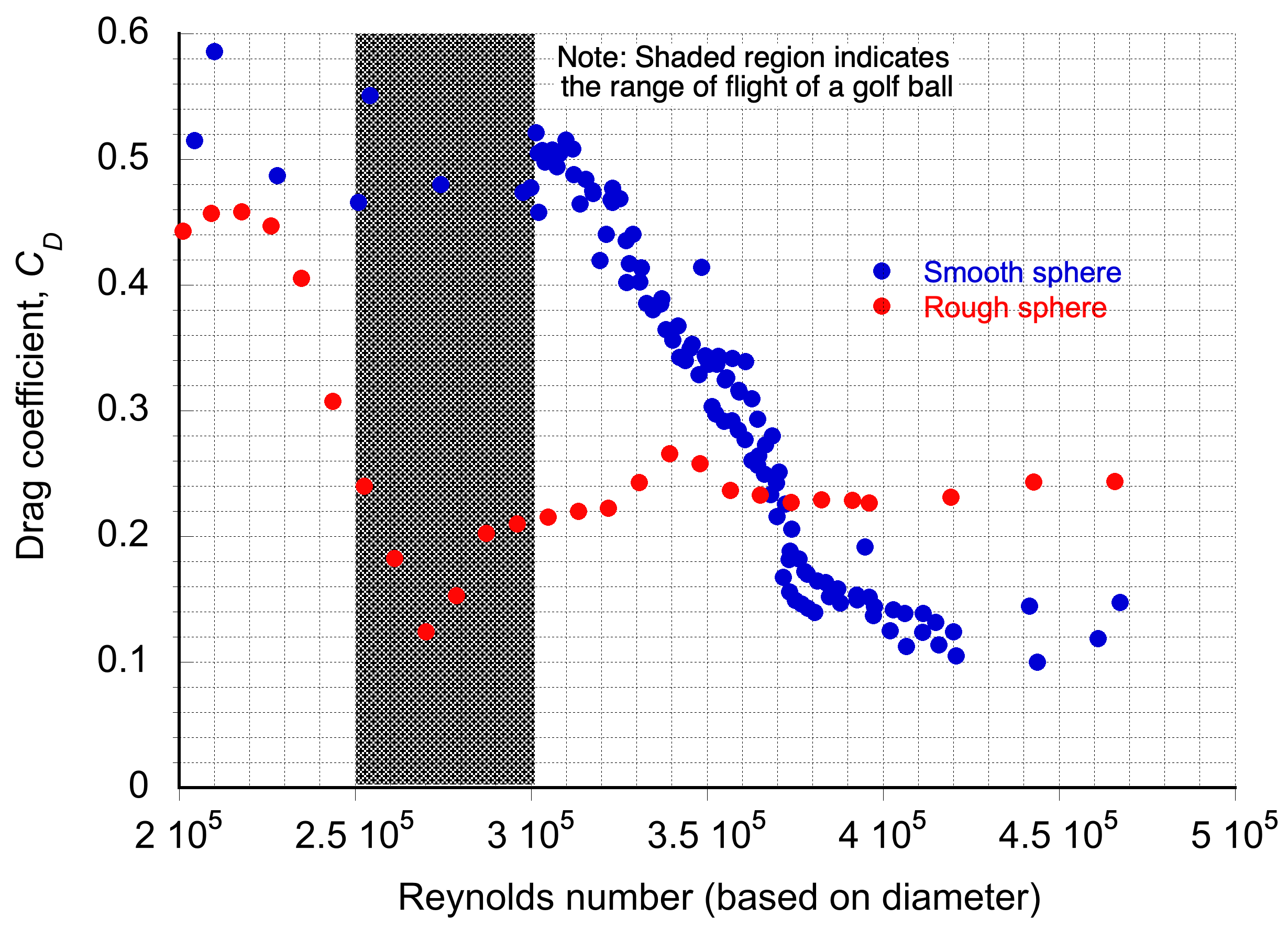
Examining the versus Reynolds number for this range, as shown in the graph below, it can be seen that based on measurements then, the drag coefficient of a rough ball in this range will be less than half of a smooth ball, i.e., the dimples act to increase in the effective Reynolds number. Of course, this outcome is supported by experience and other empirical data from golfing.
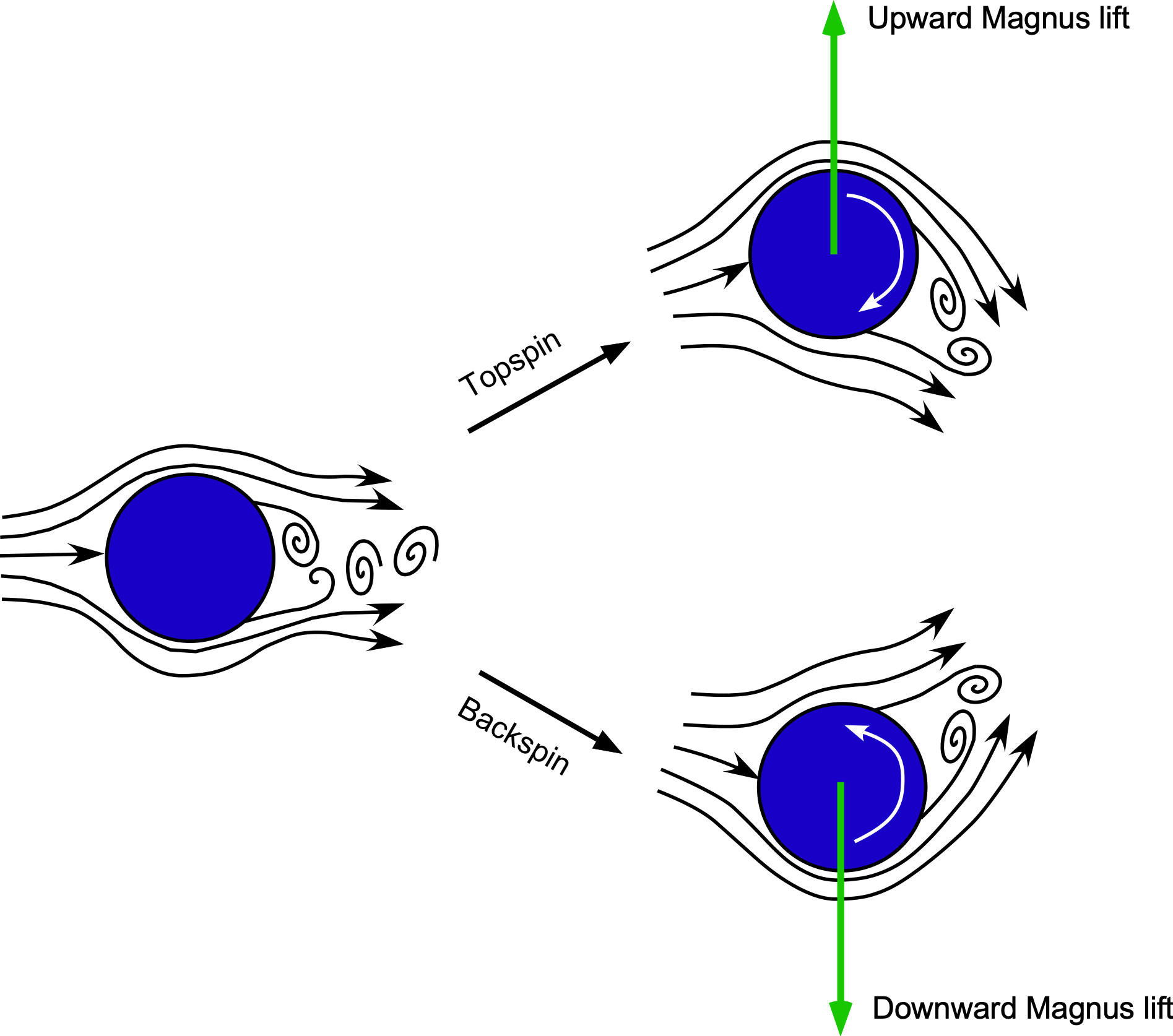
Aerodynamics of Spinning Balls
Another effect experienced by golf balls and other balls used in various games and sports is a lift force produced by their spinning motion, such as backspin or topspin. The ball’s spin spoils the flow’s horizontal symmetry, creating differential pressure and producing a lift force. This phenomenon is known as the Magnus effect, named after Heinrich Magnus, the German scientist who first studied it in the 19th century, as illustrated in the figure below. In some cases, Magnus observed a tendency of a cannonball to curve or veer significantly away from their expected flight path. He concluded that this behavior was a result of the residual spinning motion of the cannonball as it left the barrel. Isaac Newton also observed this same behavior while watching people play tennis.
The dependence of the Magnus lift coefficient,  , on the translational and rotational speeds of a smooth cylinder of diameter
  has been investigated and measured in the wind tunnel, some results being reproduced in the figure below, where
  is its translational speed and
  is the rotational angular velocity. The results are presented in terms of a non-dimensional spin rate,
  . Notice the additional dependency on the Reynolds number, as given by
  . A negative lift or a so-called “reverse” Magnus effect occurs at or about the critical Reynolds number. This behavior is attributed to a “moving wall” effect that affects the boundary layer characteristics over the top and bottom halves of the cylinder, resulting in premature laminar separation on the upper half and delayed separation on the lower half. This latter behavior is also characteristic of spheres and balls.
 , on the translational and rotational speeds of a smooth cylinder.
Therefore, the explanation for the curving behavior of a ball lies in aerodynamics. In the case of a topspin, there is a higher flow velocity (hence a lower pressure) over the ball’s upper surface, thereby producing a positive (upward) lift force. Therefore, a topspin will cause a ball to fly higher but not always further. A backspin will cause a ball to dive more quickly toward the ground. Backspin and topspin effects are utilized in various other ball games, such as golf, baseball, and soccer, which enhance the player’s skill and the game’s unpredictability, ultimately adding to the fun. The effects of Reynolds number and surface roughness mean that the curving characteristics depend on the size and surface finish of the ball; for example, a smooth ping pong ball versus the seams found on a baseball or soccer ball.
Complex Three-Dimensional Bluff Bodies
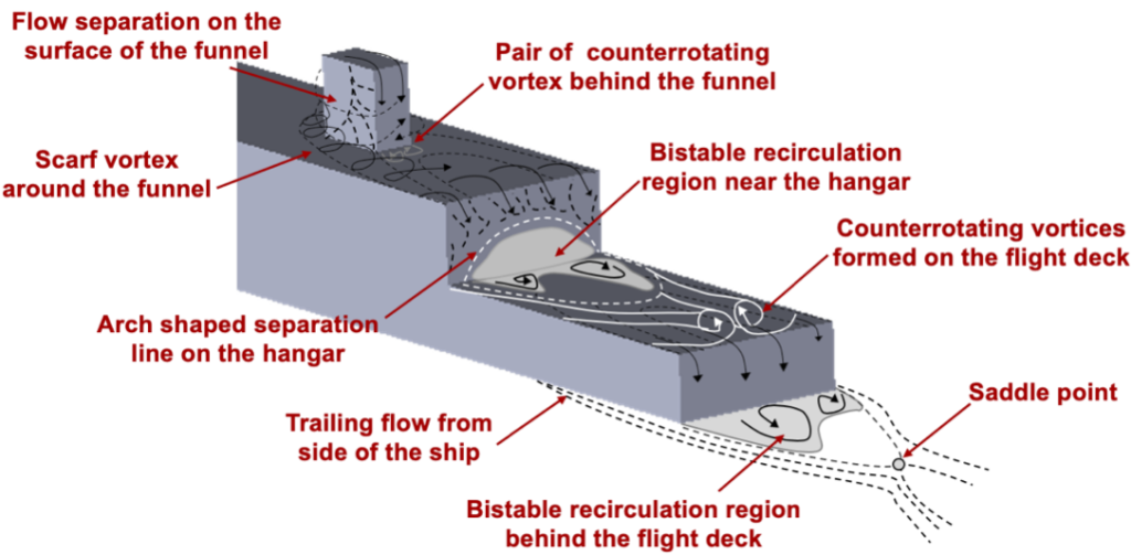
The flows produced about more general three-dimensional bluff body shapes are considerably more complex, and some of the other types of flow phenomena involved are shown in the figure below, which describes the behavior of the so-called “airwake” produced over the surface of a ship. Scarf or horseshoe vortices tend to form and wrap around the base (or foot) of bluff bodies that protrude from a surface (wall), in this case, the funnel. These vortices are, again, another source of drag. In addition, complex flow separation and reattachment regions on the body often make the a priori estimation of drag on such bodies very difficult.
Vortex-Induced Vibration
One of the concerns with three-dimensional bluff body flows is that the aerodynamics can produce such high forces to cause excitations of the structure it is made of. One of the most concerning effects in this regard is vortex-induced vibration (VIV), where the aerodynamic excitation produced by vortex shedding causes the structure to vibrate or even flutter. VIV problems can occur in many engineering applications, not just limited to the aerospace field, where flow-induced vortex shedding is possible, particularly with long, slender cantilevered structures such as wires, chimneys, and suspension bridges.
The Strouhal number is usually used to quantify VIV effects, which relates the frequency of shedding to the velocity of the flow and a characteristic dimension of the body (diameter in the case of a cylinder). The Strouhal number  is defined as
(9) 
where  is the vortex shedding frequency (or the frequency in radians per second), and is the freestream flow velocity. The Strouhal number of a cylinder is 0.2 and is constant over a wide range of Reynolds numbers.
The lock-in phenomenon occurs when the vortex-shedding frequency becomes close to a system or structure’s natural vibration frequency, resulting in a severe oscillation or even flutter. Although the onset of flutter will usually always reach a limit cycle in some form, the associated high cyclic stresses produced on a metallic structure can quickly cause fatigue failure.
Wakes Shed from Bridges
In civil engineering, vortex shedding from suspension bridges, which are bluff bodies in cross-section, is a significant cause of concern and can lead to bridge failures. When the Tacoma Narrows Bridge over Puget Sound in Washington state collapsed in 1940 because of a torsional flutter caused by a stiff wind, it was captured on film. The lessons learned have become a textbook example of vortex-induced vibration. However, this bridge is one of many that have suffered from the effects of VIV and flutter.
The figure below shows the essence of the problem. The bluff “H” shape of the bridge’s cross-section causes vortex shedding, resulting in periodic, unsteady aerodynamic forces. This behavior causes the bridge deck to twist in the wind, as shown in the figure below. Depending on the bridge’s characteristics, such as weight and dynamic frequencies, the deformations can be substantial and may quickly exceed 20 degrees.
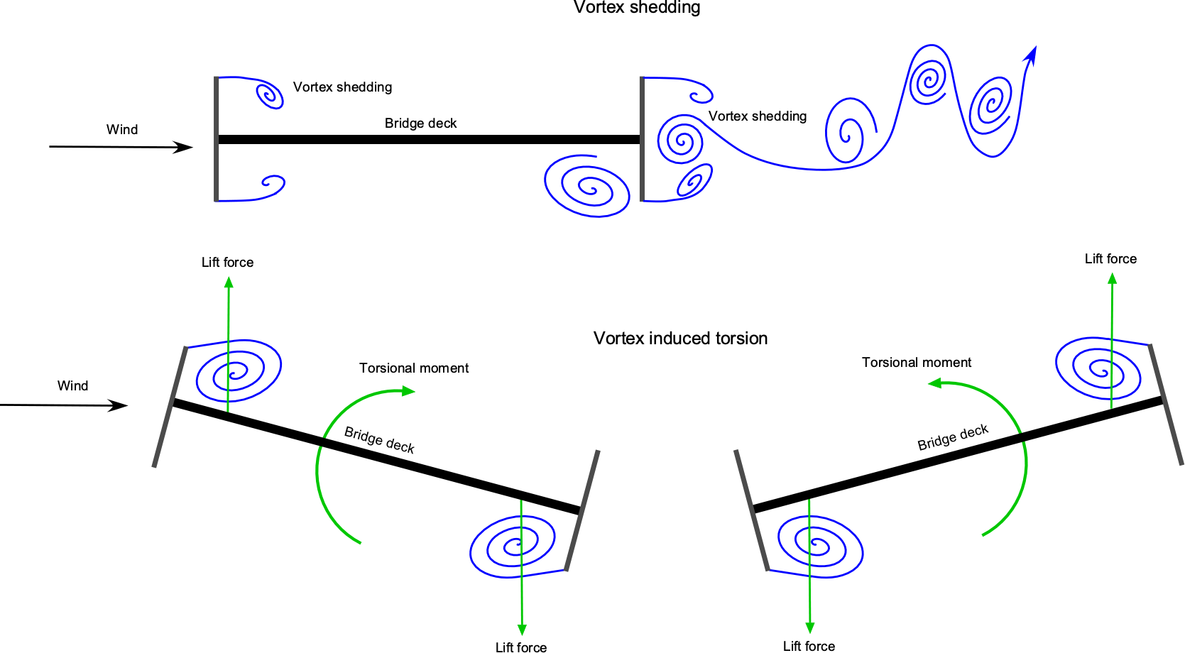
The twisting of the bridge deck increases the flow separation, forming stronger vortices and higher aerodynamic loads that further twist the deck. While the deck structure resists this lifting and twisting because of its inherent torsional stiffness, this behavior can lead to a “lock-in” event and the development of “torsional flutter.” In some cases, it may be possible to modify the cross-sectional shape of the bridge to reduce vortex shedding and increase the wind speed, thereby mitigating torsional flutter.
Streamlining
Streamlining a bluff or an otherwise unstreamlined body shape is a very effective technique for reducing drag. For example, the basic idea is shown in the figure below. Adding a tail and/or nose fairing can significantly delay flow separation, reducing drag. A consideration, however, is that the fairing adds extra weight to the aircraft.
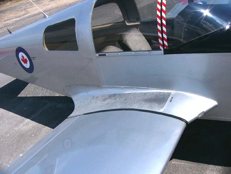
While streamlining may not be a viable engineering option in some cases because of practicality or cost, it is always a worthwhile effort on an airplane to reduce its overall drag and increase its performance, even at the expense of a slight increase in overall structural weight. For example, carefully blending a wing to the fuselage using a fairing can eliminate the horseshoe vortex and reduce interference drag from the resulting streamlining, as shown in the photograph below for a general aviation airplane, with an almost negligible increase in airframe weight. For a commercial aircraft, the wing root fairing is designed to reduce interference drag and is part of the transonic drag reduction process, utilizing Whitcomb’s area rule. The area rule states that the cross-sectional area should change smoothly and continuously, rather than abruptly, to minimize drag on an airplane; that is, the second derivative of the area change should be smooth and continuous.
An airplane with a fixed landing gear can benefit from adding fairings and spats around the landing gear and wheels. Of course, retracting the wheels entirely is the only way of almost eliminating the drag. However, the extra weight and higher cost of a mechanical system to retract the landing gear are not usually viable for smaller aircraft, such as those in the general aviation class.
Other aircraft that can benefit from streamlining include helicopters, which have relatively unstreamlined airframes for their utility. Using fairings in strategic locations on a helicopter’s airframe can reduce drag by 10% to 30%, allowing it to fly faster and/or have better flight range or endurance.
Streamlining of Terrestrial Vehicles
The aerodynamic drag of terrestrial vehicles, such as automobiles, trucks, and trains, increases significantly at higher driving speeds. For a given drag coefficient, , the drag, , on the vehicle will increase with the square of its speed , i.e.,
(10) 
So the power required to propel the vehicle  will increase with the cube of its driving speed over the ground, i.e.,
(11) 
Therefore, it is also apparent that the fuel or energy required will increase with the cube of the speed. Rolling resistance, or friction, also affects the net resistance on the vehicle and the fuel or energy needed for propulsion; however, aerodynamic effects dominate at higher speeds.
As with flight vehicles, terrestrial vehicles can reduce energy consumption by lowering drag, i.e., by streamlining to reduce the value of as much as possible. Aerospace engineers possess the training and expertise to understand the steps required to achieve profitable drag reductions. Much of the testing of terrestrial vehicles is conducted in wind tunnels, although CFD solutions can also be beneficial.
Automobiles & Cars
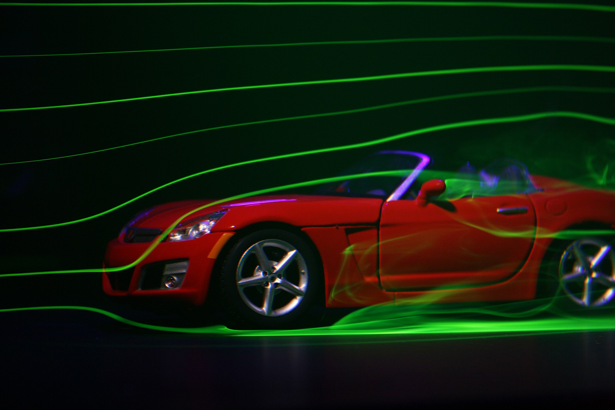
The automotive industry has become proficient in streamlining vehicles to reduce fuel consumption and internal noise, a process that typically requires extensive wind tunnel testing. Turbulence about the vehicle, such as from rear-view mirrors, can be a significant source of internal noise. The photograph below shows an example of flow visualization. The judicious use of smoke filaments and suitable lighting can provide insight into the flow patterns and where the flow is attached or separated, helping to decide where streamlining may be needed.
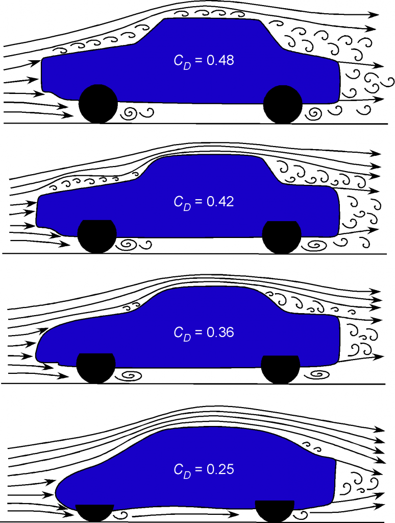
As shown in the figure below, the careful streamlining of automobile shapes can reduce drag. The result is a significant decrease in fuel consumption and notable reductions in internal noise, resulting from corresponding reductions in turbulence. However, streamlining can only be done to a point where compromises in the vehicle’s utility may become problematic. Exposed wheels are a significant drag source, so there has been a trend toward more carefully streamlining the wheel well and the vehicle’s underside.
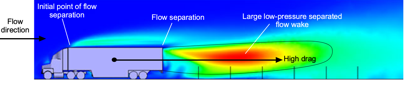
Trucks (Lorries) & Buses
As shown in the figure below, trucks (lorries) and buses are aerodynamically inefficient because of their “boxy” shapes, resulting in high base pressure drag. For most trucks, their average fuel consumption is between 50% and 200% higher than that of automobiles. For example, an 18-wheeler truck, used to transport most goods to supermarkets and similar establishments, might achieve anywhere from 5 to 8 miles per gallon (2.1 to 3.4 km per liter). Still, these values can vary significantly depending on engine size, driving speed, and the load (weight) being carried. The large, rectangular, box-like shapes often seen being towed by tractor-trailers are poor aerodynamic shapes, characterized by high drag. These boxes are typically referred to as CONEX or Intermodal Shipping Containers or ISO boxes (ISO 6346).
Engineers have four significant areas of interest in obtaining meaningful aerodynamic drag reduction on trucks and lorries. These are:
- The frontal shape of the tractor part, which is somewhat unstreamlined, is partly because of utility requirements (engine access) and cooling needs.
- The gap between the tractor’s end and the trailer’s leading edge (or the front of the CONEX container) can cause flow separation and turbulence.
- The shapes of the sides and underbody of the trailer, which shed turbulence and create drag.
- The very back of the trailer is a significant source of pressure drag.
Continuous improvements to the aerodynamics of trucks have reduced their drag, resulting in increased fuel efficiency. Minimizing the gap between the trailer and the tractor is essential, so fairings on the top of the tractor are often used, as shown in the figure below. In addition, rubber skirts can be placed underneath and along the trailer’s sides, redirecting the higher-speed airflow away from the trailer’s underside and reducing the drag from the wheels, which also act as bluff bodies.
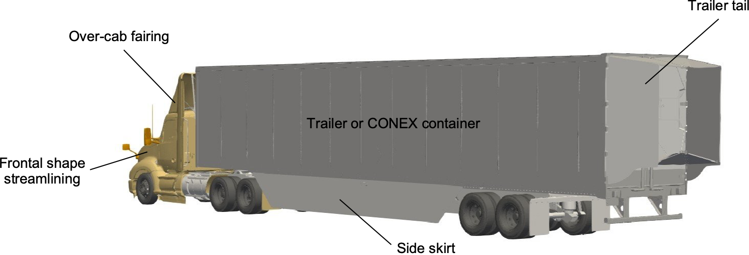
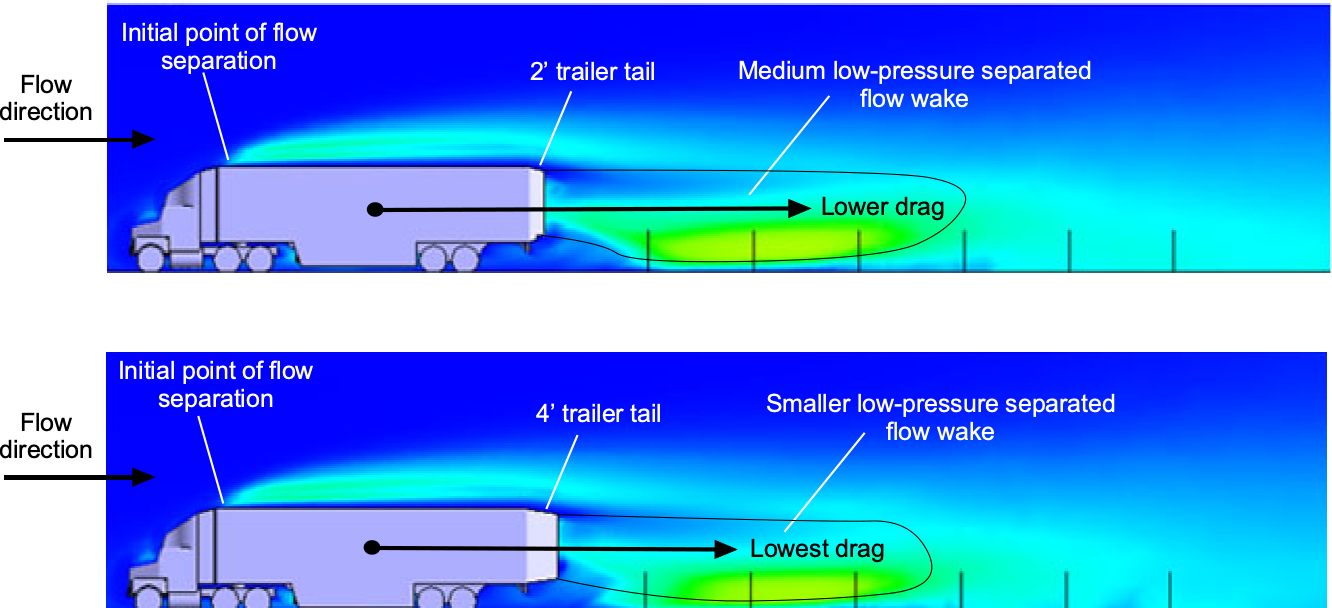
Trailer tails are increasingly used on trucks, which are pop-out afterbody fairings, as also shown in the figure above. Although relatively crude in shape, they help reduce the drag caused by flow separation and turbulence at the trailer’s rear end. The figure below shows that even a short trailer tail reduces the base pressure drag. The corresponding reduction in fuel consumption makes their use worthwhile when considering the overall fuel costs of the truck fleet. Indeed, a slight decrease in drag can significantly reduce fuel costs when the number of vehicles and the total miles traveled are considered cumulatively.
Streamlining the aerodynamics of buses and coaches is also essential in improving fuel efficiency. Manufacturers have begun introducing increasingly more streamlined shapes with minimized frontal areas and curved or tapered roofs. Spoilers, underbody skirts, and wheel covers further improve airflow management, while carefully designing doors, mirrors, and other external components helps reduce turbulence. While employing wind tunnel testing and computational fluid dynamics simulations during the design phase of a bus or coach is a significant investment in time and cost, the improved aerodynamic performance can result in substantial fuel savings and so a lower environmental impact.
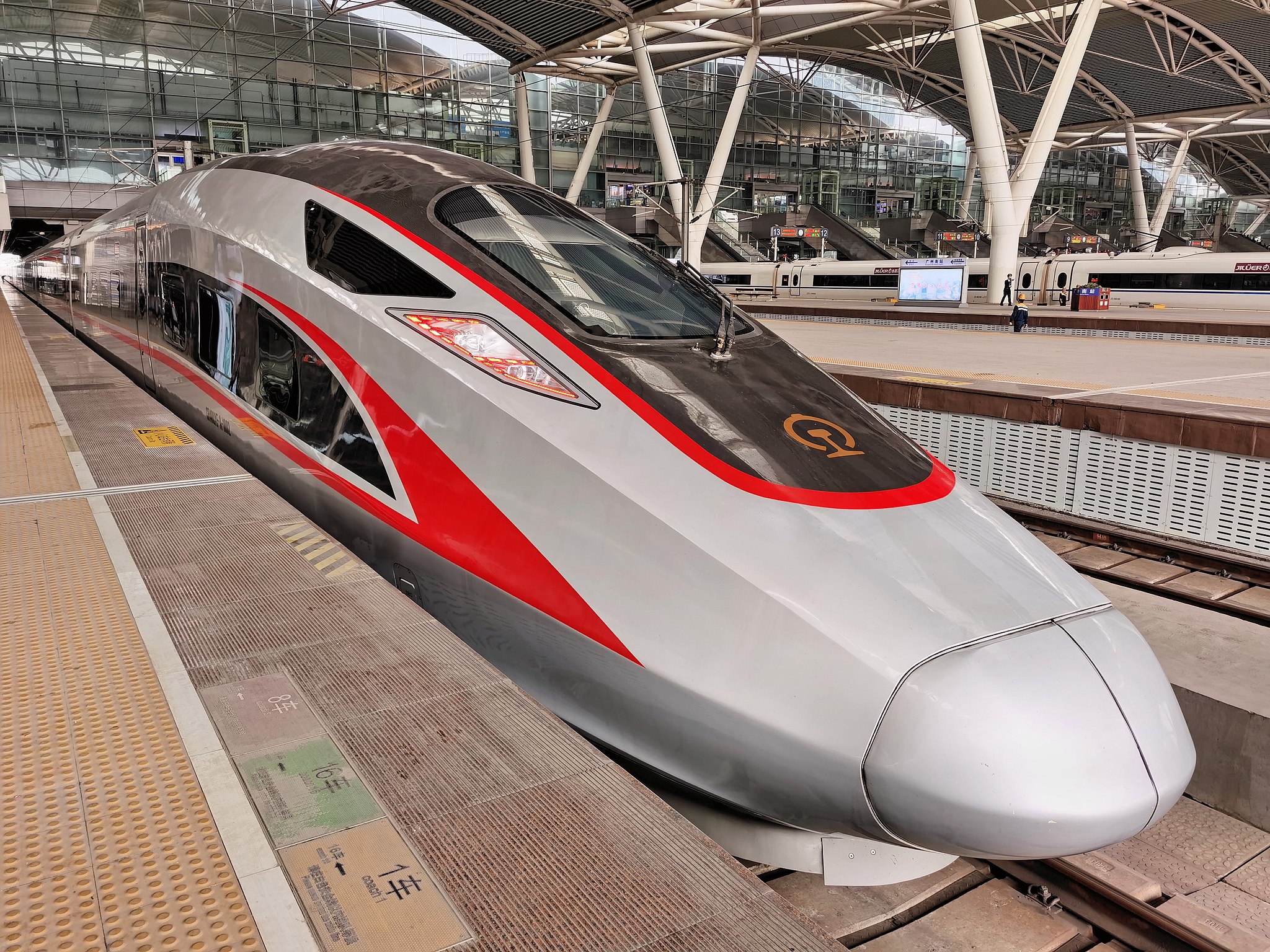
Trains
Traveling by train has long been a vital mode of transportation. High-speed railway networks continue to grow, particularly in Europe, China, and Japan. As with all vehicles, the aerodynamic drag of a train increases with the square of the speed, so power and energy requirements to propel the train increase significantly at higher speeds. Related issues for trains include the ability to supply the needed traction from the wheels to the rails and the significant pressure changes (which are felt by the passengers) when trains pass each other at high speeds or travel through tunnels.
Because the length-to-width ratio of a train is much larger than that of any other ground vehicle, the aerodynamic characteristics of trains tend to be more complex than those of cars, trucks, or airplanes. Nevertheless, significant reductions in drag can be achieved through streamlining, as shown in the photograph below. The basic principles needed are not unlike those for airplanes, including the need for a streamlined nose shape and rounded corners along the entire length of the train. Again, much of the work on the most effective steps for drag reduction on high-speed trains using types of streamlining is done in wind tunnels.
Creating Drag – Parachutes
A parachute slows an object’s motion through the air by creating drag. This situation exemplifies how creating high drag can have a positive outcome. Parachutes come in many shapes and sizes, but the classic design of a parachute canopy is a hemispherical shell, as shown in the figure below.
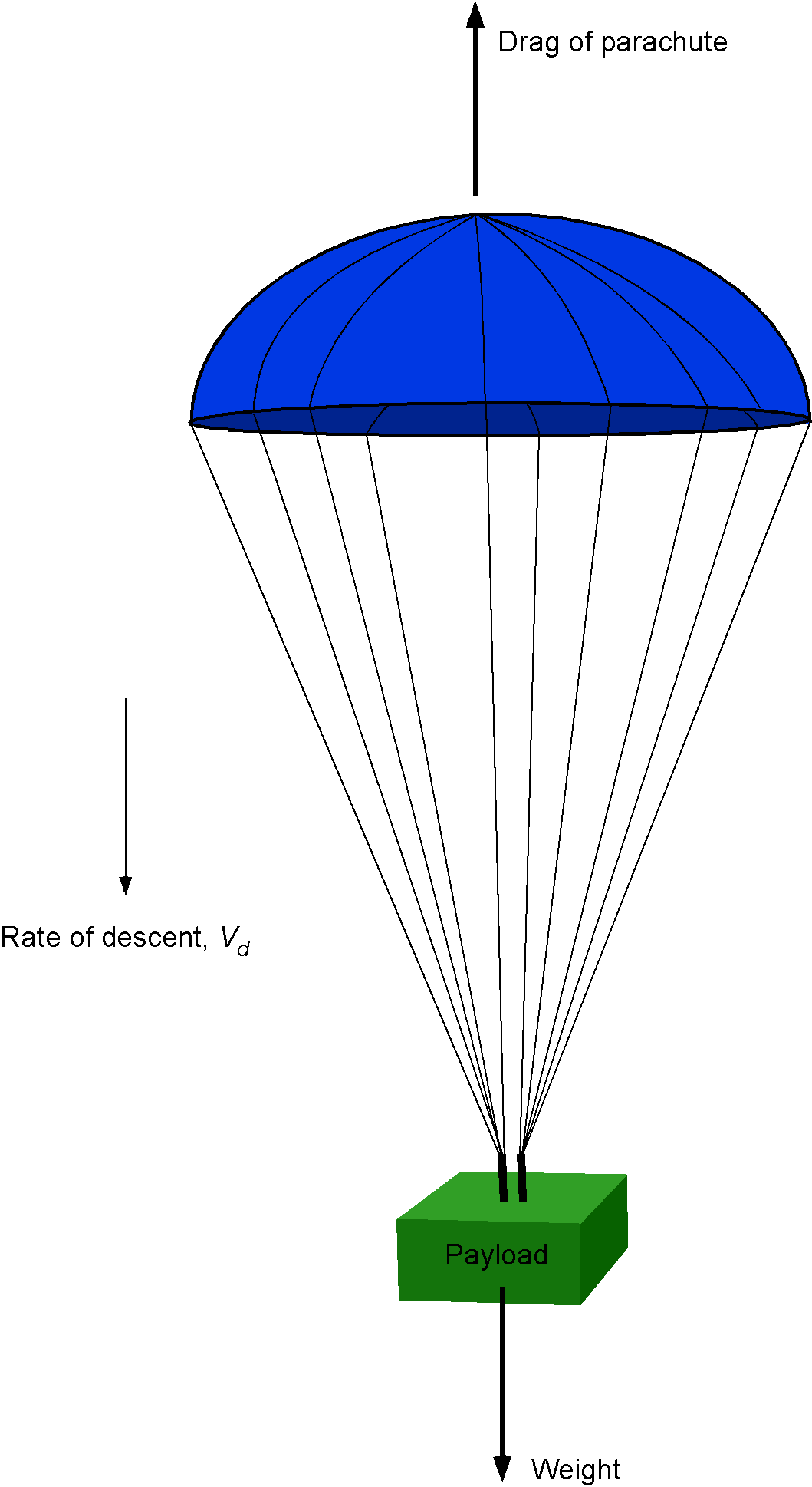
The drag coefficient of a hemispherical shell based on the projected frontal area is about 1.42. Notice that for an open hemispherical shell of diameter , its projected frontal area (i.e., the reference area on which the drag coefficient is based) is just the area of a circle of this diameter. The drag coefficient for most parachutes is close to 1.42, depending on their construction.
If the weight suspended from the parachute is  , and if the weight of the parachute itself is neglected, then steady force equilibrium gives
(12) 
where is the drag of the parachute. The drag is given by
(13) 
where is the projected frontal area of the parachute, is the density of the air, and  for an open hemispherical shell. The projected frontal area is
  , where is the diameter. Solving for (the rate of descent) gives
(14) 
Notice that the rate of descent increases for a higher weight and/or for a smaller area parachute.
For an average person, parachutes are designed to give a decent speed between 10 and 20 mph (16 and 32 kph). Of course, a more detailed analysis of this problem would consider the weight of the parachute and the backpack, although it would likely only increase the actual rate of descent by a small amount. Holes or vents can be introduced into the canopy to improve the parachute’s stability and provide it with some forward motion, which aids the parachutist in controlling the descent; the vents also slightly alter the drag coefficient.
Check Your Understanding #4 – Rate of descent of a mass with a parachute
A general aviation aircraft is equipped with a ballistic parachute recovery system for enhanced safety in the event of a severe emergency. Consider a scenario in which the aircraft’s pilot must deploy this parachute system. The aircraft has a net mass of 1,200 kg, a projected (horizontal planform) cross-sectional area of 25 m2, and a corresponding drag coefficient of 1.8 based on this reference area. The parachute has an area of 150 m2 and a drag coefficient of 1.5 based on this area. Determine the vertical airspeed at which the aircraft will parachute to a landing. Assume an average air density of 1.01 kg m-3 during the descent. Ignore the parachute’s weight and assume the aircraft descends in a flat, horizontal, wings-level attitude.
Show solution/hide solution.
The aircraft’s vertical drag coefficient is two orders of magnitude greater than expected during normal flight. In normal flight, the airplane is streamlined, resulting in minimal pressure drag and reduced boundary layer separation. However, during a vertical descent with a parachute, the airplane behaves as a bluff body with large amounts of flow separation and corresponding pressure drag.
Therefore, the net vertical drag will equal the airplane’s weight during a steady descent. The net drag will be the sum of that produced by the parachute plus that from the airplane itself, i.e.,
![\[ W = M \, g = \frac{1}{2} \varrho \, V_d^2 \, S_a \, C_{D_{a}} + \frac{1}{2} \varrho \, V_d^2 \, S_p \, C_{D_{p}} \]](https://eaglepubs.erau.edu/app/uploads/quicklatex/quicklatex.com-25bc8a84148a36c11758dfa545297ce3_l3.svg "Rendered by QuickLaTeX.com")
where  is the rate of descent,
  is the projected cross-sectional area of the airplane,
  is the drag coefficient of the airplane based on this reference,
  is the projected cross-sectional area of the parachute,
  is the drag coefficient of the parachute based on this reference area. Simplifying gives
![\[ M \, g = \frac{1}{2} \varrho \, V_d^2 \left( S_a \, C_{D_{a}} + S_p \, C_{D_{p}} \right) \]](https://eaglepubs.erau.edu/app/uploads/quicklatex/quicklatex.com-7f8ca1cc45c0a00644aecf8ec25d0f16_l3.svg "Rendered by QuickLaTeX.com")
and rearranging to solve for gives
![\[ V_d = \sqrt{ \frac{2 M \, g}{\varrho \left(S_a \, C_{D_{a}} + S_p \, C_{D_{p}} \right)}} \]](https://eaglepubs.erau.edu/app/uploads/quicklatex/quicklatex.com-de096e20b2dc997ecfecf815289cf704_l3.svg "Rendered by QuickLaTeX.com")
Substituting in the known numerical values gives
![\[ V_d = \sqrt{ \frac{2 \times 1,200.0 \times 9.81 }{1.01 \times \left(25.0 \times 1.8 + 150.0 \times 1.5 \right)} } = 9.29 \mbox{ m/s} \]](https://eaglepubs.erau.edu/app/uploads/quicklatex/quicklatex.com-890bed3f6c3353645580903b0ef55f62_l3.svg "Rendered by QuickLaTeX.com")
which seems reasonable, but it will still be a reasonably firm landing!
Bluff Bodies at Supersonic Speeds
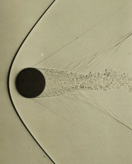
The behavior of bluff bodies at high speeds is also fascinating to aerospace engineers, especially for spacecraft re-entering Earth’s atmosphere. The drag of supersonic projectiles has been studied in wind tunnels. The results show that their drag is comprised not only of a high value of pressure drag from flow separation on the aft part of the body but also wave drag from the formation of shock waves, as illustrated in the figure below for a sphere (ball) flying at supersonic speeds. Notice the strong compression bow shock that stands off from the leading edge of the sphere, as well as the turbulence in the wake behind the sphere.
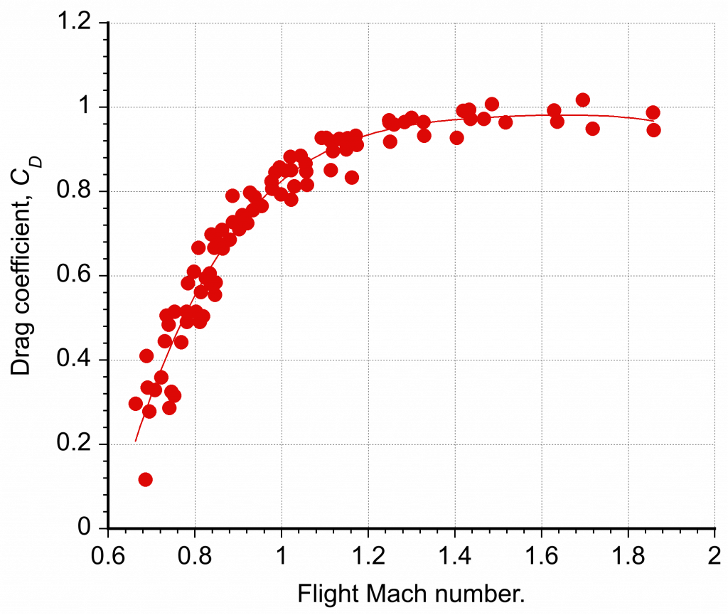
The effects of Reynolds number on the drag of a sphere have been previously discussed, but what about the effects of Mach number? The most accurate high Reynolds number data for spheres flying at Mach numbers between 0.6 and 2.0 date back to the 19th century, when Francis Bashforth conducted drag measurements on supersonically spherical projectiles between 1870 and 1880, as shown below. Interestingly, it can be seen that the drag coefficient plateaus in value for Mach numbers greater than 1.4.
H. Julian “Harvey” Allen, an aeronautical engineer at NASA, designed a spacecraft that would return to re-enter the Earth’s atmosphere. His approach recognized that bluff or “blunt” bodies moving at very high supersonic and hypersonic Mach numbers generate strong shock waves that form in front of the body, known as a bow shock, as shown in the image below. Notice that the bow shock is positioned away from the body’s surface, referred to as the standoff distance. Because there are significant changes in the temperature of the flows across strong shock waves, shock waves that stand off from the surface allow much more heat to be dissipated into the air rather than into the body itself.
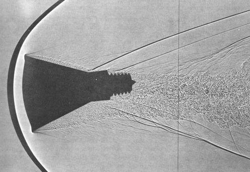
The heat transfer is related to the radius of curvature of the leading edge of the body,  , by the relationship
(15) 
Clearly, the larger (blunter) the shape, the lower the heat transfer. Also, note the significant flow separation and turbulence in the body’s wake in this image. The bluff body shape also generates significant pressure drag, helping to slow down the spacecraft as it re-enters the atmosphere until it is sufficiently slowed down for a parachute to be deployed, which is another example of how the creation of drag on a body can be beneficial.
Summary & Closure
While aerospace engineers are more often concerned with minimizing drag, using, in part, the principles of streamlining, in other cases, the creation of drag can also be beneficial. The study of bluff body shapes, with its almost infinite number of possibilities, is not just theoretical; it also has practical applications. Many standard shapes have been studied in wind tunnels, and their drag characteristics are well-known and published as functions of Reynolds number and, in some cases, Mach number as well, e.g., projectiles and re-entry vehicles, which are crucial in aerospace engineering.
The flow features and drag characteristics of angular bluff body shapes are primarily independent of variations in Reynolds number, whereas smooth bluff bodies show more sensitivity to Reynolds number. Most smooth bluff bodies (e.g., circular cylinders and spheres) have a critical Reynolds number, below and above which there is a significant change in the flow state and resulting drag behavior. Drag reduction of terrestrial vehicles remains a substantial issue in reducing fuel consumption, with conventional streamlining practices being highly effective but now reaching the point of diminishing returns. However, the future may see more innovative concepts, possibly in the form of active flow control devices, to help further reduce drag.
5-Question Self-Assessment Quickquiz
For Further Thought or Discussion
- Make a list of the parts of an airplane that are potentially bluff-body-producing drag elements. Besides removing them, what steps could be taken to reduce the drag of these elements?
- A rectangular sensor package is desired to be mounted on the external fuselage of a high-speed aircraft. What are the potential engineering concerns?
- If dimples can reduce drag on golf balls, then why are dimples not used on the surfaces of airplanes or automobiles?
- For the nose cone of a rocket, is it best to use a sharply pointed nose or a blunt, rounded nose, and why?
Other Useful Online Resources
For more information on bluff bodies, check out some of these online resources:
- Fantastic educational film on The Secret of Flight 7: Problem of Drag.
For interesting images of vortex shedding from cylinders, check out Professor Matthew Juniper’s page, which includes more readings and videos. - Fluid mechanics video lecture on bluff bodies.
- Fluid mechanics video lecture on the drag forces produced on bluff bodies.
- Inflatable trucktails for tractor-trailers!
- A CFD simulation of the supersonic flow over a bluff body.
- YouTube video on the aerodynamics of golf balls.
- Video on the intricate aerodynamics of the dimples on golf balls.
- You can find Lord Raleigh’s original paper on Aeolian tones here.
- A video of galloping power lines in a strong wind caused by vortex shedding.
