Airfoil Geometries

J. Gordon Leishman

doi:https://doi.org/10.15394/eaglepub.2022.1066.n21

24 Airfoil Geometries

Introduction

Aerospace engineers must know how to select or design suitable cross-sectional wing shapes (often called airfoil profiles or airfoils) for use on a diverse range of flight vehicles such as subsonic, transonic, and supersonic airplanes, various types of space launch vehicles, as well as helicopter rotors, propeller blades, wind turbines, unoccupied aerial vehicles (UAVs), etc. To this end, not all airfoils are created equally, and different airfoil shapes will be better suited for one application versus another. For example, airfoils for use on the wings of low-speed airplanes are generally thicker (in terms of their thickness-to-chord ratio) and have more surface curvature or camber. Airfoils for high-speed aircraft, especially for supersonic flight, are much thinner with more pointed leading edges and much less camber.

Historically, the design of airfoil shapes for specific applications has advanced through an evolutionary process, synergistically combining theoretical analysis, wind tunnel experiments, and flight testing. Engineers often begin by selecting candidate airfoil shapes with the desired characteristics and then employing mathematical models and CFD simulations to predict aerodynamic performance. Wind tunnel experiments can validate these predictions, providing empirical data for any design changes and aerodynamic refinement of the airfoil section. Subsequent flight testing may give further assessments as to the validity of the selected airfoil(s), allowing engineers to iteratively refine airfoil designs based on actual aircraft performance. Throughout this process, considerations specific to the intended application must be integrated to ensure that the optimized airfoil shapes meet the unique requirements of particular flight vehicles.

Learning Objectives

Appreciate the historical evolution of airfoil sections for aircraft applications.
Identify and explain the significance of the critical geometric parameters that define the shape of an airfoil.
Know how to construct a NACA airfoil profile geometrically using a camberline shape and a thickness envelope.
Understand the differences in the shapes between subsonic, transonic, and supersonic airfoil sections.

History of Airfoils

Historically, the most suitable airfoils for most practical engineering applications were obtained through an evolutionary process. In this regard, theory and experimentation (e.g., wind tunnel testing) have been used to design airfoils to meet specific operating requirements for different aircraft types, including low-speed airplanes, high-speed airplanes, helicopters, propellers, wind turbines, etc.

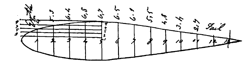
Sir George Cayley, often revered as the “Father of Aeronautics,” delineated the problem of sustentation, i.e., aerodynamic lift, from that of drag, i.e., the component of aerodynamic resistance. Cayley made essential observations about drag, including “It has been found by experiment that the shape of the hinder part of the spindle is of as much importance as that of the front in diminishing resistance;” Cayley referred to the shape of a wing as spindle-shaped. Cayley obtained the profile shown in the drawing below by measuring the cross-sectional shape of a trout, which, interestingly enough, conforms closely to modern low-drag “laminar” airfoil sections.

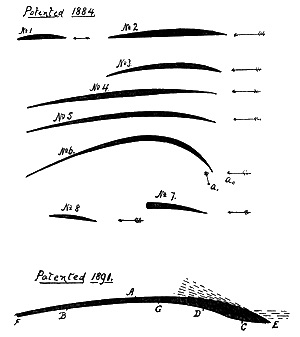
Cayley’s sketch of the cross-section of a trout looks remarkably like a modern airfoil section. Taken from “*Aeronautical & Miscellaneous Note-Book of Sir George Cayley*,” Cambridge University Press, 1933.

Some of the earliest known airfoil sections considered for aircraft concepts were patented in the 1880s by Horatio Phillips, as shown in the figure below, which were inspired by the wings of birds. Taking inspiration from nature is nothing new in engineering, but history shows that it should not necessarily be a basis for our engineering. Notice the thin, highly cambered profile shapes, which are now known to have poor aerodynamic efficiency compared to modern airfoils, at least under the operating conditions of most flight vehicles. Phillips also tested these airfoils in one of the very first wind tunnels.

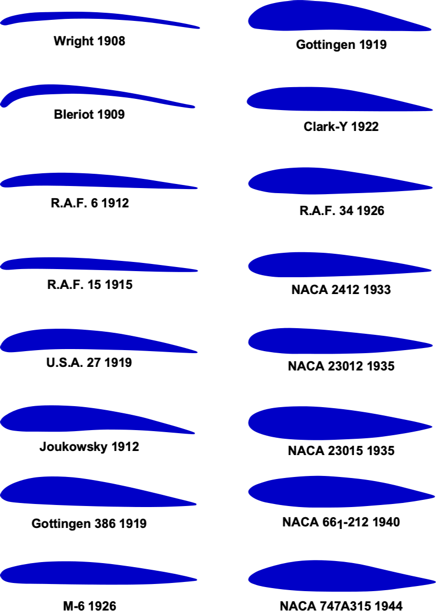
Some of the earliest known “concavo-convex” airfoil shapes were patented in the late 1880s.

Not long after Phillips, Gustave Eiffel conducted more experiments using a wind tunnel of the open-return (single passage) type. The Wright brothers also built and used an open-return wind tunnel that would prove instrumental to the success of their 1903 Flyer, recognizing that not only the airfoil cross-section was important for wing efficiency but also the wing span-to-chord ratio, known as the aspect ratio. The figure below shows a relatively rapid evolution of airfoil shapes tailored to aircraft applications between 1908 and 1944, with the thin and highly cambered airfoil sections used on early airplanes being relegated to history.

Early airfoil shapes were improved systematically but empirically by trial and error over many decades using a combination of testing in the wind tunnel and theoretical developments.

Wind tunnel work to measure airfoil characteristics was soon followed by the first development of validated numerical methods to predict chordwise pressure distributions and airfoil characteristics without making as many measurements in the wind tunnel. The computational tools to help design airfoils that produce specific aerodynamic characteristics first became available in the 1920s. The development of the thin-airfoil theory by Max Munk (in the U.S.) and Hermann Glauert (in the U.K.) during the 1920s led to a better understanding of how the camber affected an airfoil’s lift and pitching moments.

The problem of defining the airfoil pressure distribution for an airfoil with thickness and arbitrary shape was tackled by Theodorsen & Garrick in the early 1930s. The design of practical airfoil profiles was further aided by methods such as the conformal transformation first developed by Prandtl & Tietjens. This latter approach made it possible to compute pressure distributions and the resulting lift and pitching moment characteristics of some specially shaped “Joukowski” airfoils. The aerodynamic properties of Joukowski airfoils were measured in wind tunnel tests starting in the late 1920s at Gottingen in Germany and by the NACA in the U.S.A. from 1930 onward.

Today, it is possible to predict the aerodynamic characteristics of airfoils with a high confidence level using several popular computer codes, such as XFoil, which are freely available in the public domain. Even today, however, measurements of airfoil characteristics in wind tunnels have proven more reliable than results from calculations, mainly when the airfoils operate at higher angles of attack, higher subsonic and transonic Mach numbers, or lower Reynolds numbers.

There are thousands of airfoils in current use, most selected or otherwise adapted to optimize their performance for their specific flight vehicle application. A common question is what airfoil section(s) is (are) used on particular aircraft. Jane’s All The World’s Aircraft is a good source for civil aircraft, often requiring a university library trip. A comprehensive online list of airplanes and the airfoil(s) that they use has also been prepared.

Design Requirements

Design requirements for airfoil sections are essential to ensure optimal performance in various applications such as aircraft wings, tail surfaces, and other aerodynamic surfaces. The specific design requirements may vary depending on the intended use and performance objectives, but here are some typical design considerations for airfoil sections:

Obtaining high values of the maximum attainable lift coefficient before flow separation and stall occur.
The minimization of drag over a broad range of operating conditions.
The attainment of a particular value of nose-up or nose-down pitching moment.
The ability to reach high values of the lift-to-drag ratio, perhaps also at specific angles of attack.
A high critical Mach number, i.e., the free-stream Mach number when supersonic flow first develops over the airfoil.
Good lift-to-drag ratio in supersonic flight over a broad range of angles of attack.

There has recently been much interest in designing efficient airfoils for use at the very low flow speeds and low Reynolds numbers found on UAV systems. These require detailed knowledge of boundary layer developments, including laminar to turbulent boundary layer transition. Unfortunately, airfoil characteristics at low Reynolds numbers are usually quite different from those at higher Reynolds numbers, often showing remarkably low aerodynamic efficiencies.

Airfoil Geometry

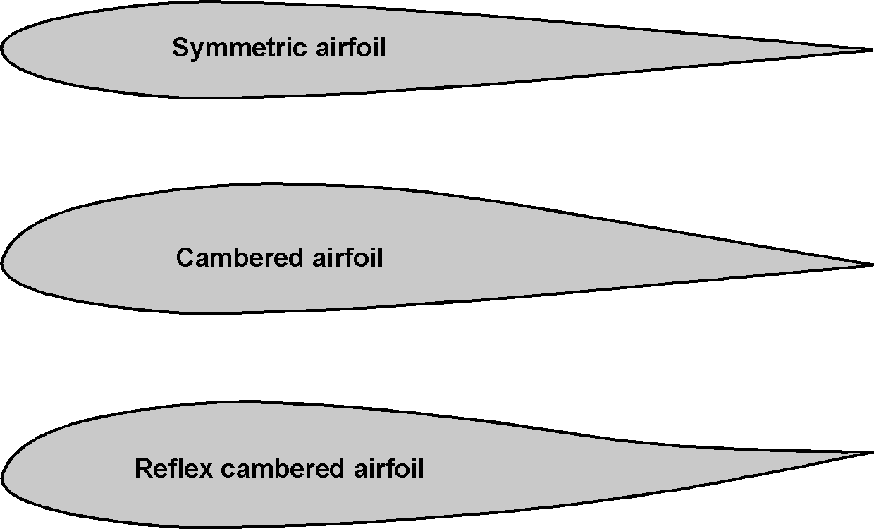
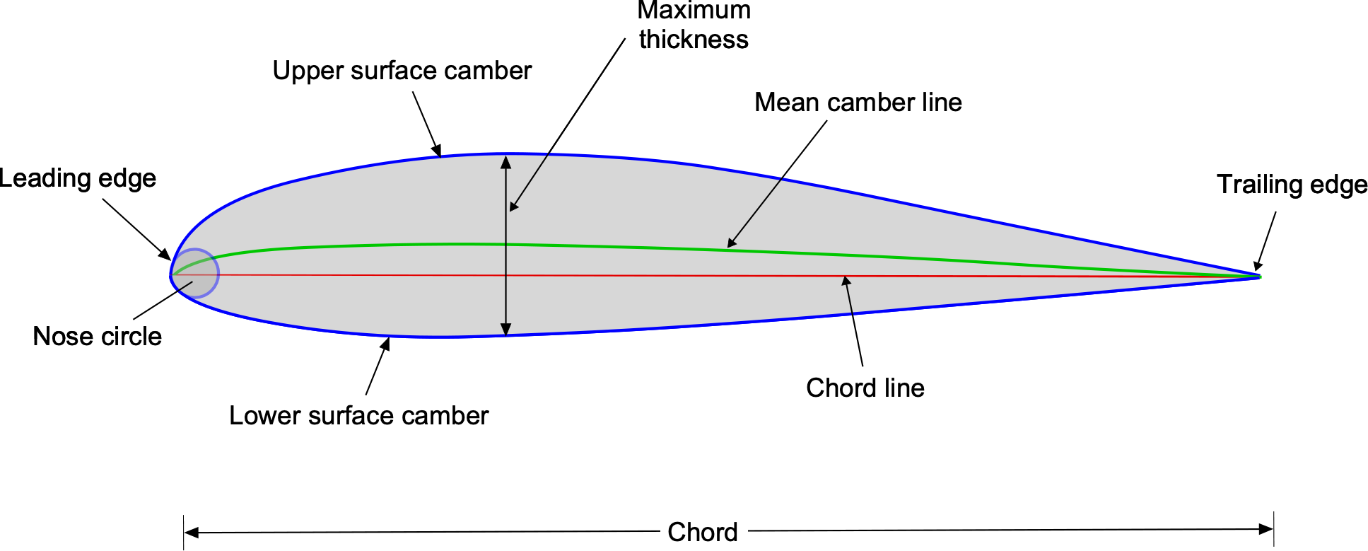
The basic geometry of an airfoil is described in terms of a profile shape or envelope that defines the curvature of its upper and lower surfaces. As shown in the figure below, airfoils can be symmetric, which is an airfoil with the same shape and curvature on the upper and lower surfaces, or cambered, which has a different upper and lower surface shape. In addition, some airfoils have camber in which the trailing edge region has an upward or negative camber, called reflex camber, often used on flying wings, helicopters, and autogiros.

Airfoils can be symmetric or cambered. Cambered airfoils with upturned trailing edges are called “reflexed” airfoils.

As shown in the following figure below, the critical length dimension of an airfoil profile is defined in terms of its chordline; the chord is defined as the distance measured from the leading edge of the airfoil profile to its trailing edge. However, in the geometric construction of airfoil profiles, it is necessary to be more precise about how exactly the profile shape is defined, including the value and position of the maximum thickness (thickness-to-chord ratio), the value and position of the maximum camber, as well as the nose shape or radius.

An airfoil shape is defined in terms of curvature (camber) and thickness distribution.

In most geometric constructions of airfoil profiles, the airfoil’s thickness envelope is defined so that the envelope’s upper and lower camber surfaces evolve if the thickness is plotted perpendicular to the slope of a defined mean camberline. The mean camber of the airfoil profile measures its average curvature, and the shape and amount of the mean camber will also affect the shapes and curvature of the airfoil’s upper and lower surfaces. There is a formalized geometric process to trace out the envelope in terms of the coordinates of the upper and lower profile shapes, which can also be tabulated for various purposes such as plotting, the creation of a CFD grid, or for CAD/CAM. In addition, the leading-edge shape of the airfoil is often defined geometrically in terms of a nose radius, which also affects the airfoil’s aerodynamic characteristics.

Other geometric parameters of interest for airfoils are the maximum thickness and maximum camber, usually defined as a ratio relative to the chord, i.e., the maximum thickness-to-chord ratio and the maximum camber ratio. The chordwise position of these latter parameters may also be defined and used to describe the shape of the airfoil profile, especially as they subsequently relate to the effects on the aerodynamic characteristics of the airfoil. For example, it is known that increasing the camber at the leading edge of an airfoil can increase its maximum lift coefficient to a point, but camber will also increase pitching moments.

NACA Method of Drawing Airfoil Shapes

As early as 1920, research institutions in Europe and the U.S.A. embarked on the systematic measurement of the aerodynamic characteristics of airfoils already in practical use. This work led to organizing the results into families of airfoils known to produce specific aerodynamic characteristics. With a catalog of airfoils with measured aerodynamic characteristics, aircraft designers could quickly choose the most appropriate airfoil profile for their particular application.

The National Advisory Committee for Aeronautics, or the NACA, which is always pronounced as “N-A-C-A” and never “NACA,” conducted the most comprehensive and systematic study of the effect of airfoil shape on aerodynamic characteristics. Existing cambered airfoils, such as the Clark-Y and Gottingen sections, were known from the earliest wind tunnel experiments to have good aerodynamic characteristics. Therefore, the NACA used these airfoils as a basis; these two airfoils had geometrically similar profiles when the camber was removed, and the airfoils were reduced to the same thickness-to-chord ratio. A polynomial curve fit defined the resulting thickness shape, which became fundamental to many of the subsequent NACA airfoil families, i.e., what has become known as the classic NACA 00-series symmetric airfoils.

Geometric Construction

In the NACA method of defining the shape of an airfoil, a coordinate system is placed at the nose of the airfoil and is defined in terms of the $x$ and $y$ distances, as shown in the figure below. The airfoil profile is then constructed of a series of upper and lower points by using a thickness shape $y_t(x)$ distributed around a camber line $y_c(x)$ and by plotting the thickness perpendicular to the slope of the camberline, as detailed in the lower part of the figure.

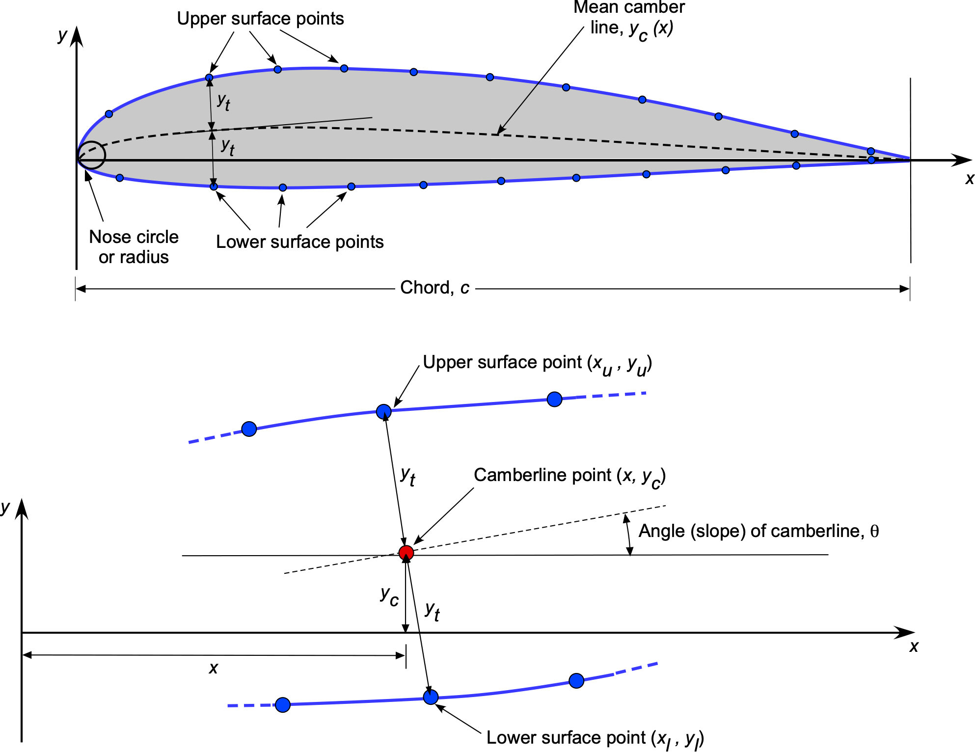
The NACA method of constructing airfoils uses a standard thickness envelope plotted perpendicular to the slope of the camberline.

The basic steps of the process are straightforward geometry and easily programmed on the computer. If the slope of the camberline makes an angle $\theta$ with the chord line, as shown in the figure above, then the upper coordinate $(x_u, y_u)$ and lower coordinates $(x_l, y_l)$ of the airfoil can be obtained by using the equations

(1) $\begin{eqnarray*} {x}_{u} & = & {x} - {y}_{t} \sin \theta \\[6pt] {y}_{u} & = & {y}_{c} + {y}_{t} \cos \theta \\[6pt] {x}_{l} & = & {x} + {y}_{t} \sin \theta \\[6pt] {y}_{l} & = & {y}_{c} - {y}_{t} \cos \theta \end{eqnarray*}$

The slope angle, $\theta$ , of the camberline is given by

(2) $\begin{equation*} \theta = \arctan{\left(\frac{dy_{c}}{dx}\right)} \end{equation*}$

where $y_c (x)$ expresses the shape of the camberline. For airfoils with small camber, i.e., small values of surface slope angle $\theta$ , applying the thickness along the $y$ axis is a reasonable approximation.

It is usually preferred to plot airfoils using non-dimensional coordinates such that $\overline{x} = x/c$ and $\overline{y} = y/c$ , i.e., coordinates non-dimensionalized with respect to the chord, $c$ , so that

(3) $\begin{eqnarray*} \overline{x}_{u} & = & \overline{x} - \overline{y}_{t} \sin \theta \\[6pt] \overline{y}_{u} & = & \overline{y}_{c} + \overline{y}_{t} \cos \theta \\[6pt] \overline{x}_{l} & = & \overline{x} + \overline{y}_{t} \sin \theta \\[6pt] \overline{y}_{l} & = & \overline{y}_{c} - \overline{y}_{t} \cos \theta \end{eqnarray*}$

where $\overline{x} = x/c$ and $\overline{y} = y/c$ , i.e., the coordinates are non-dimensionalized with respect to the chord, $c$ . The slope angle, $\theta$ , of the camberline is given by

(4) $\begin{equation*} \theta = \arctan{\left( \frac{d \,\overline{y}_{c}}{d \, \overline{x}} \right)} \end{equation*}$

where $\overline{y}_{c} (\overline{x})$ expresses the shape of the camberline.

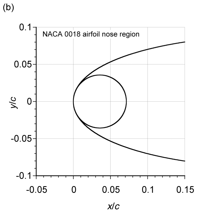
Nose Radius

The nose curvature or radius, $r_t$ , must also be formally located on the profile and is obtained with an inscribed circle. The center for the leading edge radius (defined by a circle) is found by drawing a straight line through the end of the chord at the origin of the axes, but with a slope equal to the slope of the camberline at $\overline{x}=0.005$ , and then moving a distance along this line equal to the leading edge radius, as shown in the figure below. The resulting point then becomes the origin location for the leading-edge nose circle. Notice that the center of the nose circle will not lie on the mean camberline.

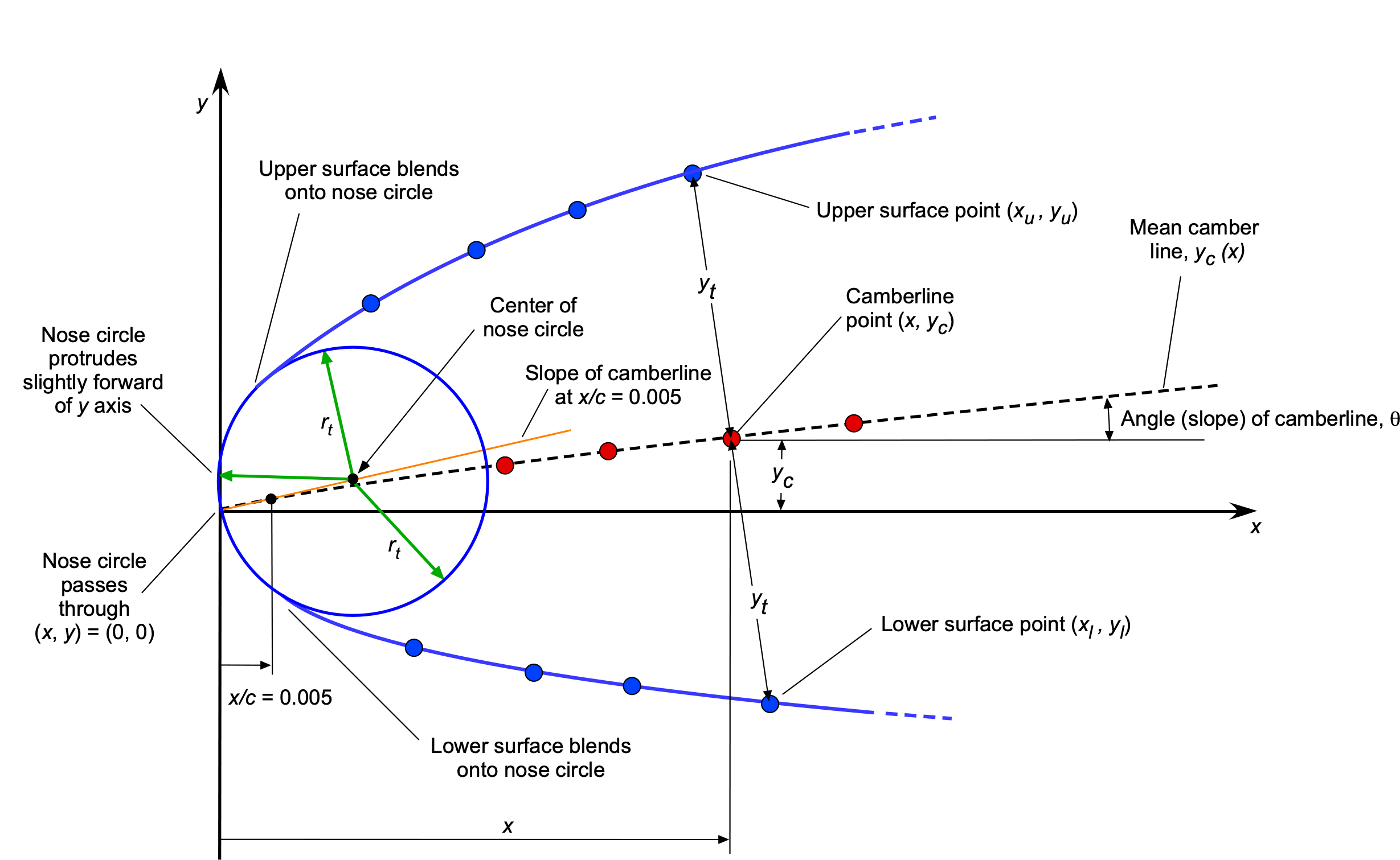
Notice also that as an artifact of this construction, the leading edge of the airfoil shape protrudes very slightly forward of the $y$ -axis, but this effect is of no practical significance. For a symmetric airfoil, the center of this nose circle lies on the $x$ -axis. For all cases, the nose circle is drawn and geometrically blended into the upper and lower surface coordinates; some care should be taken in conducting this process numerically.

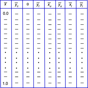
Airfoil Coordinates

The various upper and lower surface points can be exported to a data file, as shown in the figure below, and the airfoil’s final shape is then obtained by connecting the points. Generally, more points will be needed in the nose region of the airfoil because of the section’s higher curvature. To give a reasonable approximation of the shape, 100 points should be used. A CFD grid or a CNC machine file may need 500 to 1,000 points across the chord. It will be noticed that the NACA airfoils are designed to have a finite thickness at their trailing edge, which is for manufacturing reasons.

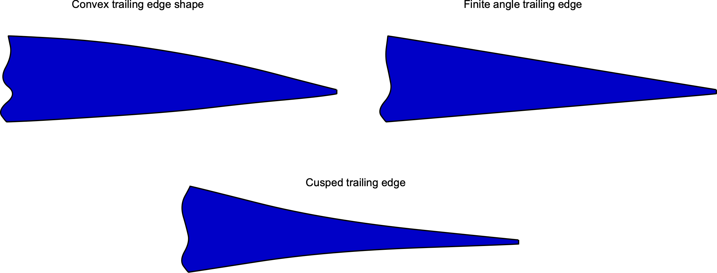
The coordinates of the airfoil shape in the form of a table, which can be saved as a data file for various applications.

Trailing-Edge Shapes

It may be noted that airfoil sections can have various trailing edge shapes. The three general trailing edge shapes found in practice are convex, finite angle, and cusped, as shown in the figure below. All these trailing edge shapes will have a finite thickness, meaning they are not infinitely thin but have some thickness when implemented on an actual wing or airfoil. The convex trailing edge curves outward, away from the airfoil surface. This trailing edge has a sharp edge, forming an angle with the airfoil surface; it terminates at a finite angle. Finite angle trailing edges are commonly used in certain airfoil designs where specific aerodynamic characteristics are desired. A cusped trailing edge features a sharp, pointed shape resembling a cusp. This trailing edge type is less common and is typically used in specialized airfoil designs where precise control over flow separation is required. The choice of trailing edge shape depends on the specific requirements of the aerodynamic design, maximum lift, minimum drag, and stall characteristics.

Circle Method of Airfoil Construction

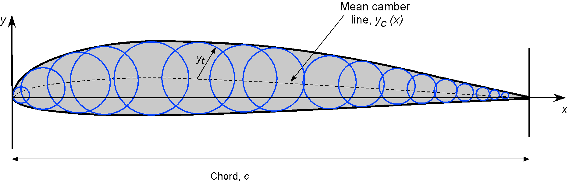
Another way of drawing an airfoil section graphically is to draw it as a series of circles of radius $y_t$ (or $\overline{y_t} = y_t / c$ ) if done non-dimensionally as a fraction of chord) centered on the camberline, as shown in the figure below. The upper and lower surfaces of the airfoil are then formed from curves drawn tangential to all of the circles. While this method offers a simple way of graphical construction, which can be a helpful approach in visualizing the overall process of drawing an airfoil section, it is best to construct the shapes of the surfaces and tabulate the data points, as mentioned previously.

Another way of drawing an airfoil is by using a series of circles centered along the camberline. Curves drawn tangent to the circles define the upper and lower surfaces.

Connection to Aerodynamic Characteristics

The forgoing NACA approach also allowed the systematic construction of several families of airfoil sections differing only by a single geometric parameter, such as the camber, the location of the maximum camber, the maximum thickness to chord ratio, and the location of this value. The primary geometric characteristics that affect the airfoil characteristics include the maximum camber and its distance aft of the leading edge and the leading-edge nose curvature (nose radius) airfoil. The various families of airfoils developed by NACA were then tested in the wind tunnel to measure the effects of varying the critical geometrical parameters on the lift, drag, and pitching moment characteristics as a function of angle of attack, as well as in some cases, the chord Reynolds number and Mach number.

It was a monumental undertaking by the engineers at NACA, and even today remains the most definitive catalog of aerodynamic measurements on low-speed airfoil sections. A summary of the results is documented in considerable detail in the NACA report (later a book) “Theory of Wing Sections, Including a Summary of Airfoil Data,” by Ira H. Abbott and A. E. von Doenhoff.

“Theory of Wing Sections, Including a Summary of Airfoil Data,” by Ira H. Abbott and A. E. von Doenhoff.

Symmetric NACA Airfoils

Symmetric airfoil sections are often selected for horizontal and vertical tail surfaces on airplanes and other aircraft. The upper ( $+y_t$ ) and lower ( $-y_t$ ) surfaces of the NACA 00-series or four-digit symmetrical sections are described by the polynomial

(5) $\begin{equation*} \pm\overline{y}_t = 5 \overline{t} \bigg( A \sqrt{\overline{x}} \! - \! B \left( \overline{x} \right) \! - \! C \left( \overline{x}\right)^{2} \! + \! D \left(\overline{x}\right)^{3} \! - \! E \left(\overline{x}\right)^{4} \bigg) \end{equation*}$

where $\overline{x} = x/c$ , $\overline{y_t} = y_t/c$ , and $t/c = \overline{t}$ , i.e., the geometry of the airfoil and the coordinates are expressed as a fraction of its chord or for $c = 1$ . The coefficients $A$ through $E$ were obtained by a curve fit to the best-known airfoils when they were all reduced to the same thickness-to-chord ratio. They are given by: $A = 0.2969$ , $B = 0.1260$ , $C = 0.3516$ , $D = 0.2843$ and $E = 0.1015$ . The factor of $5 \overline{t}$ is used to scale the coordinates to the correct thickness-to-chord ratio.

The shape of the airfoil is then obtained by plotting $\overline{y}$ as a function of $\overline{x}$ and for any number of points, at least 50 points and, more typically, 100 points will be required to define the airfoil shape to good fidelity. The corresponding leading-edge circle of the airfoil is given by

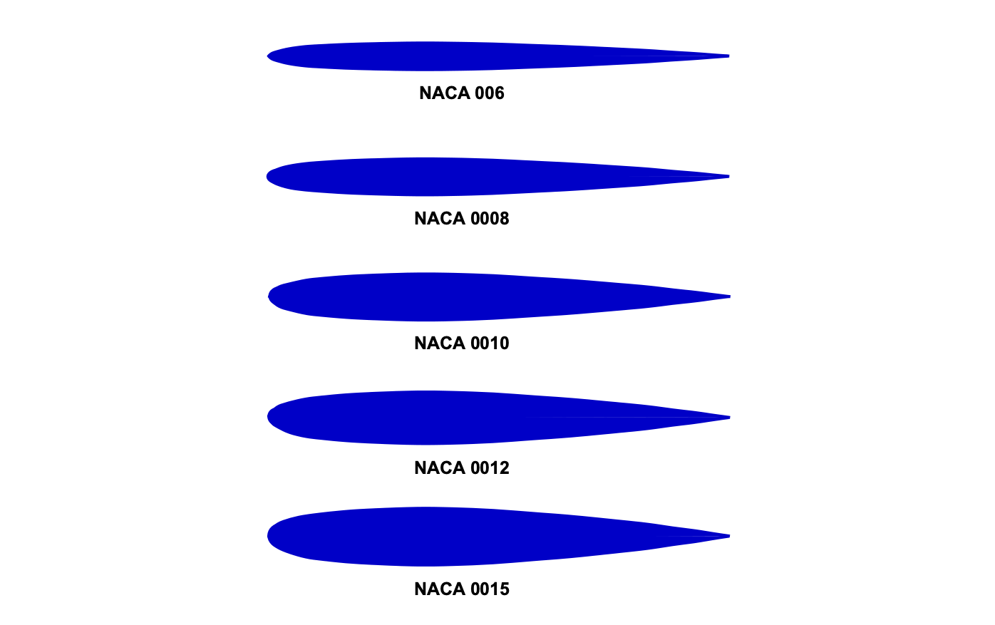
(6) $\begin{equation*} r_{t} = 1.1019 \, \overline{t}^{~2} \end{equation*}$

which is smoothly blended into the upper and lower surfaces to give a circular arc shape at the leading edge, as previously described. Examples of the NACA 00-series symmetric airfoils are shown in the figure below. The number denotes the thickness-to-chord ratio in percent of the chord; e.g., a NACA 0015 has a 15% thickness-to-chord ratio, which means $\overline{t} = 0.15$ .

Examples of NACA 00-series symmetric airfoil sections. The number denotes the thickness-to-chord ratio in percent of chord; e.g., a NACA 0015 has a 15% thickness-to-chord ratio.

Cambered NACA Airfoils

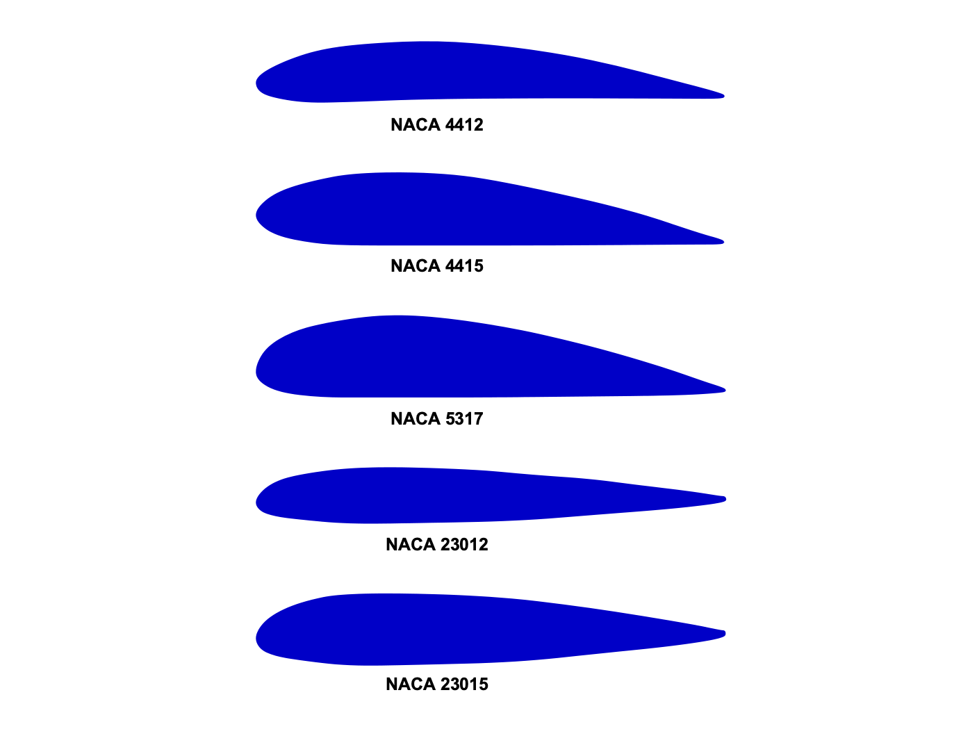
As previously discussed, cambered airfoils are constructed by distributing the thickness envelope (as defined above) around a mean camberline shape. The camberline shape $y_c$ is specified as a function of $x$ , i.e., $y_c = y_c(x)$ . Precisely, the thickness envelope is plotted perpendicular to the camberline to trace out the profiles of the upper and lower surfaces. There are many camber line profiles in the NACA portfolio, including the two-digit and three-digit camber lines, some examples of which are shown in the figure below. The first two digits define the amount of camber, and chordwise location of maximum camber, e.g., the NACA 2408 has a 2% camber, the maximum camber location is at 40% of the chord length, and the airfoil is 8% thick.

NACA 4-digit airfoils where the 4-digit number defines the shape.

NACA Two-Digit Camberlines

The simplest cambered airfoils are used to form the NACA 4-digit series, which is comprised of the standard NACA four-digit thickness envelopes and the following camberline based on two coefficients, i.e.,

(7) $\begin{equation*} {\displaystyle \overline{y}_{c}=\left\{{\begin{array}{ll}\displaystyle {{\frac {m}{p^{2}}}\left(2p\,\overline{x} -\overline{x} ^{2}\right)} &\mbox{~for $0\leq \overline{x}\leq p$} \\[20pt] \displaystyle {{\frac {m}{(1-p)^{2}}}\left((1-2p)+2p\, \overline{x} -\overline{x}^{2}\right)} & \mbox{~for $p< \overline{x}\leq 1 $} \end{array}}\right.} \end{equation*}$

where $m$ is the maximum camber (100 $m$ is the first of the four digits), $p$ is the location of the maximum camber, with 10 $p$ being the second digit in the NACA 4-digit airfoil description. Notice the camberline is in two parts, one for the front part of the airfoil and the other for the rear. The slopes of the camberline are

(8) $\begin{equation*} {\displaystyle {\frac{dy_{c}}{dx} = \left\{{\begin{array}{ll}\displaystyle {{\frac {2m}{p^{2}}}\left(p-\overline{x}\right)} & \mbox{~for $0\leq \overline{x} \leq p$}\\[20pt] \displaystyle {{\frac{2m}{(1-p)^{2}}}\left(p -\overline{x} \right)} &\mbox{~for $p < \overline{x}\leq 1 $} \end{array}}\right.}} \end{equation*}$

NACA Three-Digit Camberlines

The NACA three-digit mean (camber) lines are also very popular and are given in this case in terms of two equations and three coefficients, i.e.,

(9) $\begin{equation*} \overline{y}_{c}=\left\{ \begin{array}{ll} \displaystyle{\frac{1}{6} k_{1} \bigg( \overline{x}^{3} - 3 m \overline{x}^{2} + m^{2}(3 - m)\overline{x} \bigg) } & \mbox{~for $0\leq \overline{x} \leq m$} \\[20pt] \displaystyle{\frac{1}{6} k_{1} m^{3} \left( 1- \overline{x} \right) } & \mbox{~for $m < \overline{x} \leq 1$} \end{array} \right.\ \end{equation*}$

where the coefficients of the camberline are given in the table below. Notice, again, that the camber line is expressed in two parts.

Mean Line	$p$	$m$	$k_1$
210	0.05	0.0580	361.4
220	0.10	0.1260	51.64
230	0.15	0.2025	15.957
240	0.20	0.2900	6.643
250	0.25	0.3910	2.230

The forward and aft slopes of the camberline are

(10) $\begin{equation*} \displaystyle { \frac{dy_{c}}{dx} } =\left\{ \begin{array}{ll} \displaystyle{\frac{1}{6} k_{1} \bigg( 3 \overline{x}^{2} - 6 m \overline{x} + m^{2}(3 - m) \bigg) } & \mbox{~for $0\leq \overline{x} \leq m$} \\[20pt] \displaystyle{-\frac{1}{6} k_{1} m^{3} } & \mbox{~for $m < \overline{x} \leq 1$} \end{array} \right.\ \end{equation*}$

Other NACA Airfoils

Modifications to the NACA four-digit and five-digit series of airfoil sections include reflex camber to produce zero pitching moment and changes in the nose radius and position of thickness to improve the maximum lift capability. The latter sections are denoted by a two-digit suffix, such as the NACA 0012-64 and NACA 23012-64. After the dash, the first integer indicates the relative magnitude of the nose radius, with a standard nose radius denoted by the number 6 and a sharp radius by 0. The second digit indicates the position of the maximum thickness in tenths of the chord.

NACA 3-Digit 231-Series Reflexed Airfoils

The camberline for the NACA 3-digit 231-series reflexed airfoils are of some interest because they are designed to give zero-pitching moments about the 1/4-chord axis. In this regard, they are considered suitable for rotor blades (e.g., for a helicopter or an autogiro) because they need to keep torsional twisting moments on the blades to a minimum. The camberline of these airfoils is defined by two equations, i.e.,

(11) $\begin{equation*} \overline{y}_{c} =\left\{ \begin{array}{ll} \displaystyle{ \frac{k_1}{6} \bigg( \left( \overline{x} - m \right)^3 - \frac{k_2}{k_1} \left( 1 - m\right)^3 \, \overline{x}- m^3 \, \overline{x} + m^3 \bigg)}~\mbox{~for $\overline{x} \le m$} \\[20pt] \displaystyle{ \frac{k_1}{6} \bigg( \frac{k_2}{k_1} \left( \overline{x} - m \right)^3 - \frac{k_2}{k_1} \left( 1 - m \right)^3 \, \overline{x} - m^3 \, \overline{x} + m^3 \bigg)}~\mbox{~for $m < \overline{x} \le 1.0$} \end{array} \right.\ \end{equation*}$

where $m = 0.217$ , $p = 0.15$ , $k_1 =15.793$ , and $k_2/k_1 = 0.00677$ .

The slopes of the camberline are

(12) $\begin{equation*} \displaystyle { \frac{dy_{c}}{dx} } =\left\{ \begin{array}{ll} \displaystyle{ \frac{k_1}{6} \bigg( 3 \left( \overline{x} - m \right)^2 - \frac{k_2}{k_1} \left( 1 - m\right)^3 - m^3 \bigg) } ~\mbox{~for $\overline{x} \le m$} \\[20pt] \displaystyle{\frac{k_1}{6} \bigg(\frac{3 k_2}{k_1} \left( \overline{x} - m \right)^2 - \frac{k_2}{k_1} \left( 1 - m \right)^3 - m^3 \bigg)}~\mbox{~for $m < \overline{x} \le 1.0$} \end{array} \right.\ \end{equation*}$

NACA Six-Digit Series

Another set of NACA airfoils that have seen some use on various aircraft is the six-digit series. These airfoils were designed to achieve lower drag, higher drag divergence Mach numbers, and higher maximum lift coefficients. Their profiles are such that they are conducive to maintaining an extensive run of laminar flow over the leading-edge region, thereby lowering skin friction drag, at least over a range of angle of attack limited to low lift coefficients.

This latter goal is achieved using camberlines that produce a more uniform pressure loading from the leading edge to a distance $\overline{x}=a$ . After that, the loading decreases linearly to zero at the trailing edge. The favorable pressure gradients tend to give the airfoils lower drag than other airfoils, at least over a limited range of attack angles. Unfortunately, surface contaminants or other transition-causing disturbances quickly spoil the characteristics of laminar flow types of airfoils, sometimes resulting in significant adverse characteristics.

Many designator combinations are used in the NACA six-digit airfoil number system, which tends to become rather complicated. For example, consider the NACA 64 $_3$ -215 $a=0.5$ section. In this case, the number 6 denotes the airfoil series, and the number 4 represents the position of minimum pressure in tenths of the chord for the basic symmetric section. The number 3 denotes the range of lift coefficient in tenths above and below the design lift coefficient for which low drag may be obtained. The number 2 after the dash indicates a design lift coefficient of 0.2, and the number 15 denotes a 15% thickness-to-chord ratio.

Grid Generation for CFD

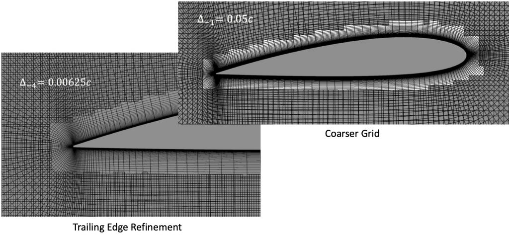
The numerical generation of airfoil coordinates can also generate input points, grids, or meshes to calculate their aerodynamic characteristics using programs like XFoil or other methods such as computational fluid dynamics (CFD). CFD grids are composed of discrete cells over which the conservation laws of fluid mechanics can be applied. An example of a grid about an airfoil section is shown in the figure below. Refinement of the grid is needed near the airfoil surface to resolve the thin boundary layers. Grid refinement may also be required at the trailing edge to model the merging of the upper and lower surface boundary layers and the development of the downstream wake.

Examples of CFD grids used to calculate the flow about an airfoil section.

The resulting flow solution can then be used to calculate various properties around the airfoil, including local pressure, local Mach number, etc. CFD methods can also be used to design the shape of an airfoil to obtain a specified level of performance. However, this tends to be lengthy because of its iterative nature and slow numerical convergence. Nevertheless, the ability to design airfoil shapes on the computer, to a point, is much quicker than the repetitive testing of many prospective shapes in the wind tunnel.

The grid generation process for CFD solutions can take on a variety of types, including structured and unstructured. Structured grids are geometrically regular, whereas unstructured grids have more randomly generated points, which is a valuable approach that can reduce the computational time needed to find a flow solution. Several software tools are available to engineers to help create grids about particular airfoil shapes. The fidelity of the resulting aerodynamic solution strongly depends on the grid, especially the number of grid points, which can reach many millions. Of course, the numerical cost (and time) to obtain a solution increases commensurately with the number of grid points.

Supersonic Airfoils

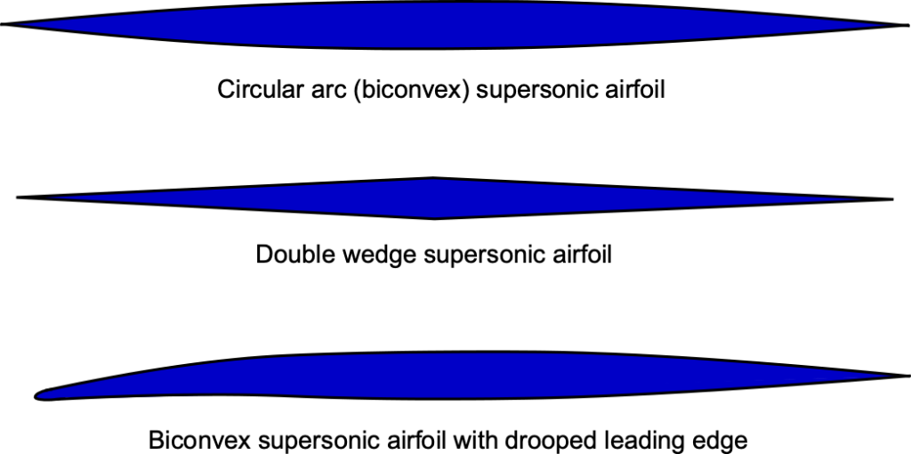
The well-rounded, cambered airfoil sections that are well-suited to subsonic flight speed are generally inappropriate for high-speed and supersonic flight. Supersonic airfoils are distinctive in their geometric shapes in that they are thin (i.e., have a low thickness-to-chord ratio) with sharp leading edges. Supersonic airfoils generally have thinner sections formed of either angled planes called double-wedge airfoils or opposed circular arcs called biconvex airfoils, as shown below. The sharp leading edges on supersonic airfoils prevent the formation of a detached bow shock in front of the airfoil, which is a high source of drag called wave drag.

Supercritical Airfoils

Because commercial airliners have been designed to reach higher and higher cruise speeds approaching the speed of sound, i.e., for flight at transonic Mach numbers in excess of 0.8, this requirement has led to the design of a unique wing shape called a supercritical wing. A supercritical wing also uses a supercritical airfoil to reduce the strength of shock waves, thereby reducing wave drag. This principle is used in transonic wing and airfoil design to control the expansion of the flow to supersonic speed and its subsequent recompression. The upshot is a delay in the onset of supercritical flow on the upper surface of the airfoil (i.e., when the flow first becomes supersonic), reducing the wave drag for a given free-stream Mach number or, alternatively, increasing the Mach number before drag rise occurs.

As shown in the figure below, the classic supercritical airfoil shape is distinctive. It has a point of maximum thickness fairly aft on the chord, with a relatively flat upper surface with a slight camber. However, such airfoils also tend to have significant camber at their trailing edges, which compensates for the reduction of lift from the front part of the airfoil section. Supercritical airfoils were extensively studied and refined during the 1960s by Richard Whitcomb and the NACA. Today, all commercial jet airliners use a form of supercritical airfoil, which allows them to cruise with good efficiency at flight Mach numbers exceeding 0.8.

The shape of a supercritical airfoil section is distinctive in that it has a reasonably flat (uncambered) upper surface.

Laminar Flow Airfoils

Sailplanes and some other aircraft use laminar flow airfoils, which are designed to maximize the extent of the laminar boundary layer over the leading edge of the airfoil, hence substantially reducing skin friction drag. A series of airfoils called the FX-airfoils have been designed explicitly for sailplane applications by Franz Xavier “FX” Wortmann, examples being shown in the figure below.

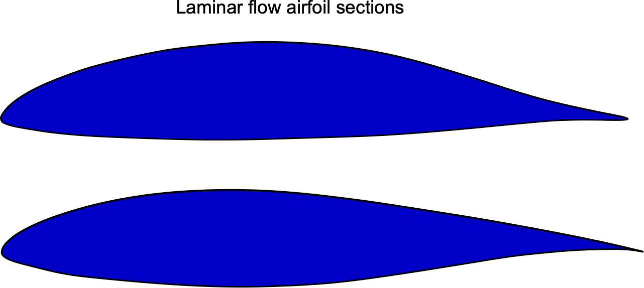
The geometric shapes of these airfoils are different from those used on most airplanes and are designed to have a point of maximum thickness close to mid-chord. This shape produces a favorable pressure gradient over the leading edge, encouraging the boundary layer to be smooth and laminar for longer. The laminar flow produces less skin friction and so less drag on the airfoil. The downside is that such airfoils typically produce lower values of maximum lift coefficient, i.e., a stall occurs at lower angles of attack. Such airfoils are also very sensitive to the surface finish, which must be glassy smooth and free of contamination (e.g., bugs) to realize the low drag values.

Examples to Try

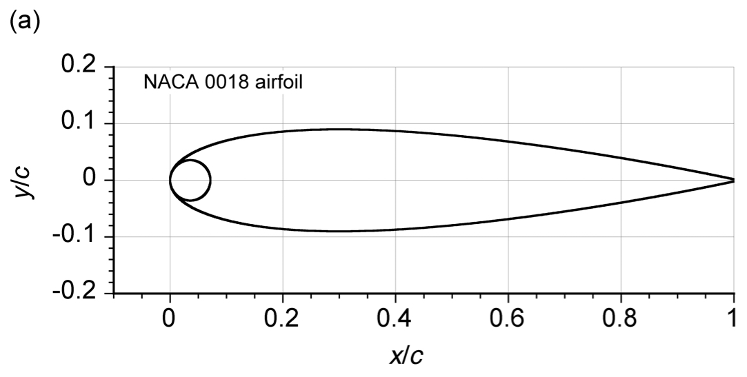
There are many airfoils to choose from, but for the student, it is valuable to understand the NACA method of geometric airfoil construction; it is very systematic and easy in terms of mathematics, and the algorithm lends itself naturally to the being programmed on the computer. For example, the shape of a NACA 0018 airfoil takes no more than to plot the shape of the upper and lower surfaces using

(13) $\begin{equation*} \!\!\!\!\!\!\!\!\!\!\!\!\!\!\!\!\!\!\!\!\!\!\!\!\!\!\!\!\!\!\!\!\pm \frac{y_{t}}{c} = \pm \overline{y} = 5 \overline{t} \bigg( 0.2969 \sqrt{\overline{x}} - \! 0.1260 \left( \overline{x} \right) - \! 0.3516 \left( \overline{x}\right)^{2} + \! 0.2843 \left(\overline{x}\right)^{3} - \! 0.1015 \left(\overline{x}\right)^{4} \bigg) \end{equation*}$

where, in this case, $t/c = \overline{t} = 0.18$ . The corresponding leading-edge radius of the airfoil is $r_{t} = 1.1019 \, \overline{t}^{2}$ .

The shape of the airfoil is obtained by plotting $\overline{y}$ as a function of $\overline{x}$ ; the results can be tabulated for any number of specified discrete points along the chord line, but 50 to 100 is usually enough for good definition, as shown in the two figures below. For practical reasons, all NACA airfoils have a finite thickness at their trailing edges, so the values of $\pm \overline{y}$ at $\overline{x} = 1$ are non-zero.

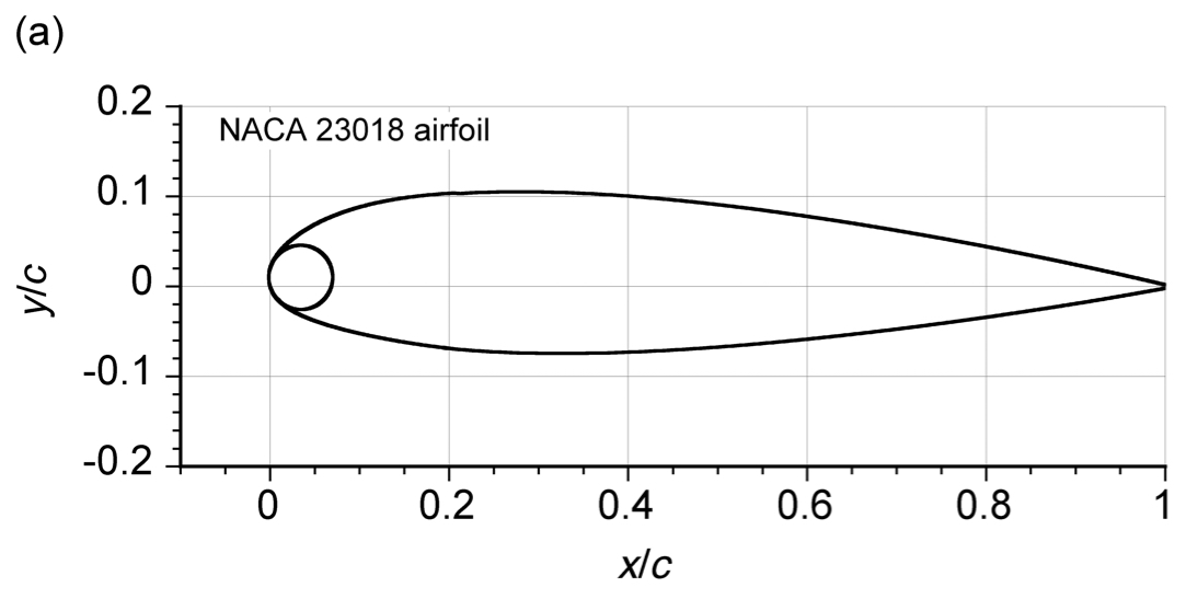
(a) Geometry of the NACA 0018 airfoil. (b) Nose detail of NACA 0018 airfoil.

The NACA 23018 airfoil section is a cambered airfoil comprised of the NACA 0018 thickness envelope (described above) wrapped around the NACA 230 mean camberline as given by

(14) $\begin{equation*} \overline{y}_{c}=\left\{ \begin{array}{ll} \displaystyle{\frac{1}{6} k_{1} \bigg( \overline{x}^{3} - 3 m \overline{x}^{2} + m^{2}(3 - m)\overline{x} \bigg) } & \mbox{~for $0\leq \overline{x} \leq m$} \\[20pt] \displaystyle{\frac{1}{6} k_{1} m^{3} \left( 1- \overline{x} \right) } & \mbox{~for $m < \overline{x} \leq 1$} \end{array} \right.\ \end{equation*}$

where $p = 0.15$ , $m = 0.2025$ and $k_1 = 15.957$ for the 230 camberline. The slope of the camber line is

(15) $\begin{equation*} \displaystyle { \frac{dy_{c}}{dx} } =\left\{ \begin{array}{ll} \displaystyle{\frac{1}{6} k_{1} \bigg( 3 \overline{x}^{2} - 6 m \overline{x} + m^{2}(3 - m) \bigg) } & \mbox{~for $0\leq \overline{x} \leq m$} \\[20pt] \displaystyle{-\frac{1}{6} k_{1} m^{3} } & \mbox{~for $m < \overline{x} \leq 1$} \end{array} \right.\ \end{equation*}$

and the slope angle of the camberline is $\theta=\tan^{-1} (dy_c/dx_c)$ . The coordinates are then

(16) $\begin{eqnarray*} \overline{x}_{u} = \overline{x} - \overline{y}_{t} \sin \theta & \mbox{~~~and~~~} & \overline{y}_{u} = \overline{y}_{c} + \overline{y}_{t} \cos \theta , \\[6pt] \overline{x}_{l} = \overline{x} + \overline{y}_{t} \sin \theta & \mbox{~~~and~~~} & \overline{y}_{l} = \overline{y}_{c} - \overline{y}_{t} \cos \theta \end{eqnarray*}$

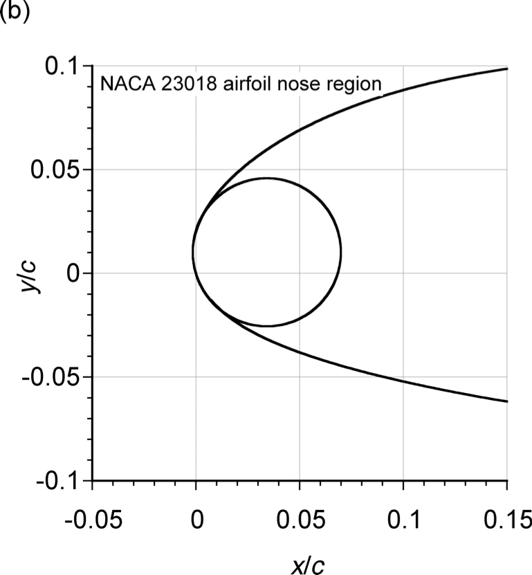
The resulting NACA 23018 airfoil is shown in the two figures below. It is apparent on the enlarged plot of the nose region that the leading-edge part of the nose radius protrudes very slightly forward of the $y$ axis; this is an artifact of the construction technique and is of no practical significance when building a wing with such an airfoil.

A MATLAB code to draw these airfoil shapes is given below. Other NACA camberlines can be examined better to understand the drawing process of NACA airfoil shapes.

MATLAB code to draw a cambered NACA 230-series airfoil

clc

clear

close all

t = 0.12;

m = 0.2025; %location of maximum camber

k1 = 15.957; %constant

r = 1.1019.*(t^2); %radius of leading edge circle

x1 = linspace(r/3,m,round(m.*500)); %x coordinates nose circle to m

x2 = linspace(m,1,round((1-m).*500)); %x coordinates m to 1

y_cam_1 = (1./6).*k1.*((x1.^3)-(3.*m.*(x1.^2))+((m.^2).*(3-m).*x1)); %camber line y coord 0 to m

y_cam_2 = (1./6).*k1.*(m.^3).*(1-x2); %camber line y coord m to 1

x = [x1 x2]; %merged x coordinates

y_cam = [y_cam_1 y_cam_2]; %merged y camber coordinates

dy_cam_1 = (1./6).*k1.*((3.*(x1.^2))-(6.*m.*x1)+((m.^2).*(3-m))); %derivative of camber line 0 to m

dy_cam_2 = -(1./6).*k1.*(m.^3).*ones(1,length(x2)); %derivative of camber line m to 1

dy_cam = [dy_cam_1 dy_cam_2]; %merged derivative of camber line

theta = atan(dy_cam); %slope of camber line

y_t = 5.*t.*((0.29690.*sqrt(x))-(0.12600.*x)-(0.35160.*(x.^2)) +(0.28430.*(x.^3))-(0.10150.*(x.^4))); %thickness equation

x_upper = x-(y_t.*sin(theta)); %x coordinates of upper surface

x_lower = x+(y_t.*sin(theta)); %x coordinates of lower surface

y_upper = y_cam+(y_t.*cos(theta)); %y coordinates of upper surface

y_lower = y_cam-(y_t.*cos(theta)); %y coordinates of lower surface

%end points to close off the trailing edge

x_end_up = x_upper(end);

x_end_low = x_lower(end);

y_end_up = y_upper(end);

y_end_low = y_lower(end);

dy_cam_005 = (1./6)*k1*((3*(0.005^2))-(6.*m*0.005)+((m^2).*(3-m)));; %derivative of camber line at x = 0.005

theta_005 = atan(dy_cam_005); %slope of camber line at x = 0.005

h = r*cos(theta_005); %center of nose circle x direction

k = r*sin(theta_005); %center of nose circle y direction

x_circ = linspace(h-r,h+r,100); %x coordinates of nose circle

y_circ_upper = sqrt((r.^2)-((x_circ-h).^2))+k; %y coordinates upper half circle

y_circ_lower = -sqrt((r.^2)-((x_circ-h).^2))+k; %y coordinates lower half circle

figure

hold on

% plot(x,y_cam,’k-‘)

plot(x_upper,y_upper,’k-‘)

plot(x_lower,y_lower,’k-‘)

plot([x_end_up,x_end_low],[y_end_up,y_end_low],’k-‘) % Close off blunt trailing edge

plot(x_circ,y_circ_upper,’k-‘)

plot(x_circ,y_circ_lower,’k-‘)

hold off

slim([-0.1 1.1])

slim([-0.2 0.2])

label(‘x/c’)

label(‘y/c’)

x0=5;

y0=5;

width=500;

height=180;

set(gcf,’units’,’points’,’position’,[x0,y0,width,height])

Summary & Closure

Using the most suitable airfoil section or sections is fundamental to the success of the design of a wing, subsonic, transonic, or supersonic, or for other applications such as rotary-wing concepts and UAVs. To this end, many different types of airfoil sections have been geometrically tailored to give the best aerodynamic performance in the conditions of flight. For example, thicker and more cambered airfoils with rounded nose shapes are more suitable for slower flight speeds and low Mach numbers. In contrast, very thin airfoils with sharp leading edges are more suitable for high speeds and supersonic Mach numbers. In addition, special supercritical airfoil sections have been developed for transonic flight conditions, where many airliners fly, to reduce wave drag and prevent boundary layer separation behind the shock wave, allowing airliners to cruise closer to the speed of sound.

5-Question Self-Assessment Quickquiz

For Further Thought or Discussion

Do some research into laminar flow airfoil sections. What geometric features are incorporated into these airfoils to produce laminar flow over the surfaces?
What kinds of airfoil shapes are likely to be used for supersonic flight? Are there any NACA supersonic airfoil sections?
Research the types of airfoils used on propeller blades. Why are different airfoils with different thicknesses along the blade span used on propellers?
What airfoils are likely to be used on wind turbines, and why?
What are the main parameters used to describe the geometry of an airfoil section?
Can you describe the concept of the chord line and camber of an airfoil section?

Other Useful Online Resources

There are many more resources on airfoils to explore:

All about airfoils on Wikipedia.
The University of Illinois at Urbana-Champagne has complied airfoil coordinates and related links. Here is the guide to many uses from the UIUC Airfoil Data site.
Go here for some interesting airfoil drawing tools.
A NASA site is about how the shape of an airfoil affects lift.
YouTube video on how airfoil shapes can affect lift generation.
Airfoil shape basics video on YouTube.
Information about grids and CFD calculations about airfoils.
Learn about Richard Witcomb’s contributions to transonic airfoil design here.

License

Icon for the Creative Commons Attribution-NonCommercial-NoDerivatives 4.0 International License

Introduction to Aerospace Flight Vehicles Copyright © 2022, 2023, 2024 by J. Gordon Leishman is licensed under a Creative Commons Attribution-NonCommercial-NoDerivatives 4.0 International License, except where otherwise noted.

Digital Object Identifier (DOI)

https://doi.org/https://doi.org/10.15394/eaglepub.2022.1066.n21