Aerodynamics of Finite Wings

J. Gordon Leishman

doi:https://doi.org/10.15394/eaglepub.2022.1066.n24

33 Aerodynamics of Finite Wings

Introduction

When the flow passes over a finite wing, i.e., a wing with a definitive span from tip to tip, the downstream flow is characterized by forming a trailing wake system comprised of swirling flows called wing tip vortices, an example shown in the photograph below. These vortices are like horizontal tornados and contain high rotational “induced” flow velocities, particularly near their centers, extending out for more than a wing span. The vortices are left in the path behind the wing, significantly affecting the airplane’s aerodynamics, primarily reducing its lift and increasing its drag. Wing-generated vortices will form along the edges of the wing tips (or at the end of the winglet) or wherever else on the wing there is a significant spanwise change in the pressure and lift distribution, such as at the side edges of the flaps.

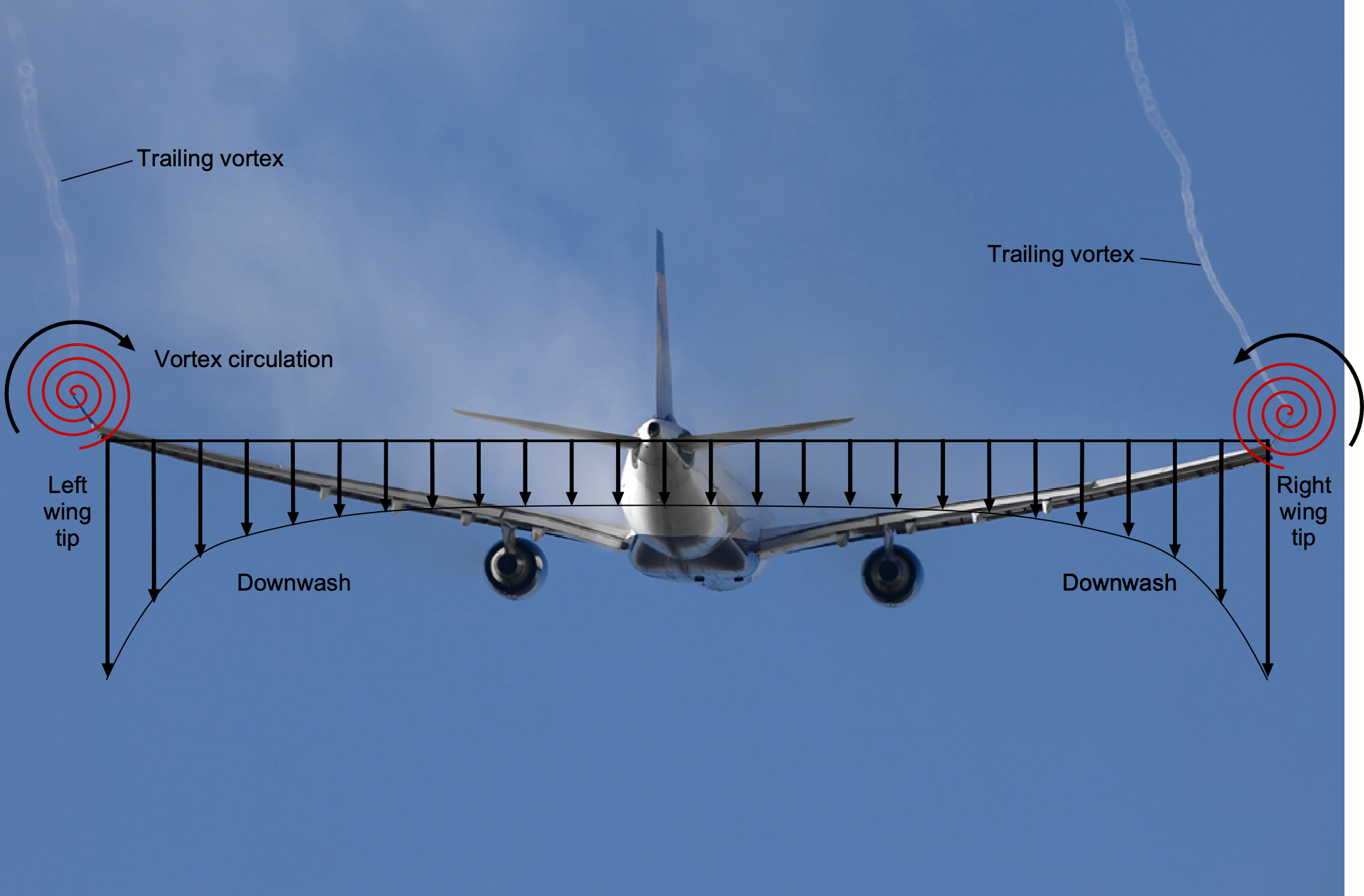
A Boeing A330 Aircraft flying away from the camera on a clear sky background. White water vapor is trailing off the wings and the winglet tips. — Natural condensation makes the flow around an airplane visible, showing the wing wake and the vortices trailing from the tips of the winglets.

The most significant aerodynamic effects of these wing tip vortices or tip vortices are on the airplane’s wing, producing a vertical downwash flow velocity over its surface, especially near the wing tips. This downwash is of sufficient magnitude to alter the angle of attack of every wing section and, subsequently, the amount of aerodynamic lift and drag produced on the entire wing. The type of drag caused by the wing tip vortices is called induced drag. Consequently, finite-span wings have different aerodynamic characteristics from those of two-dimensional airfoils. The wing’s aerodynamic characteristics, such as lift and drag, depend on its shape, including its chord distribution, span and aspect ratio, spanwise twist, and other factors, such as if the wing has a winglet. The addition of underslung engines can also affect the spanwise lift distribution and so further affect the lift and drag.

Learning Objectives

Appreciate the physical nature and effects of the trailed wake system behind a wing of finite span.
Understand the essential aerodynamic characteristics of finite wings, including the effects of wing aspect ratio on lift and drag.
Know how to interpret and use a drag polar for a finite wing and an airplane.

Origin of Trailing Vortices

The formation of vortices behind finite wings has been studied for over a century. Frederick Lanchester conducted some of the first investigations in the early 1900s, whose book on the subject eventually led to the development of modern wing theory. By any aerodynamic standard, tip vortex formation is a complex physical process. It is known that when combined with the free-stream flow, the flow in the tip region flows from the lower surface to the upper surface and begins to rotate, forming a swirling or vortical flow trailed behind the airplane.

This significant aerodynamic behavior is shown in the photograph below, which, in this case, was visualized by using smoke ejected into the wake behind a Boeing 747. The strengths of these vortical flows depend on the magnitude of the pressure gradient at the wing and the tip shape, which in turn is related to the total lift and lift distribution on the wing. A short distance downstream of the wing’s trailing edge, the outer wing tip vortices in the photograph can be seen to be rolled up rather tightly.

A Boeing 747 in a NASA trailing wake study. Two dominant swirling trailing vortices, one from each wingtip, are tightly rolled up behind the airplane.

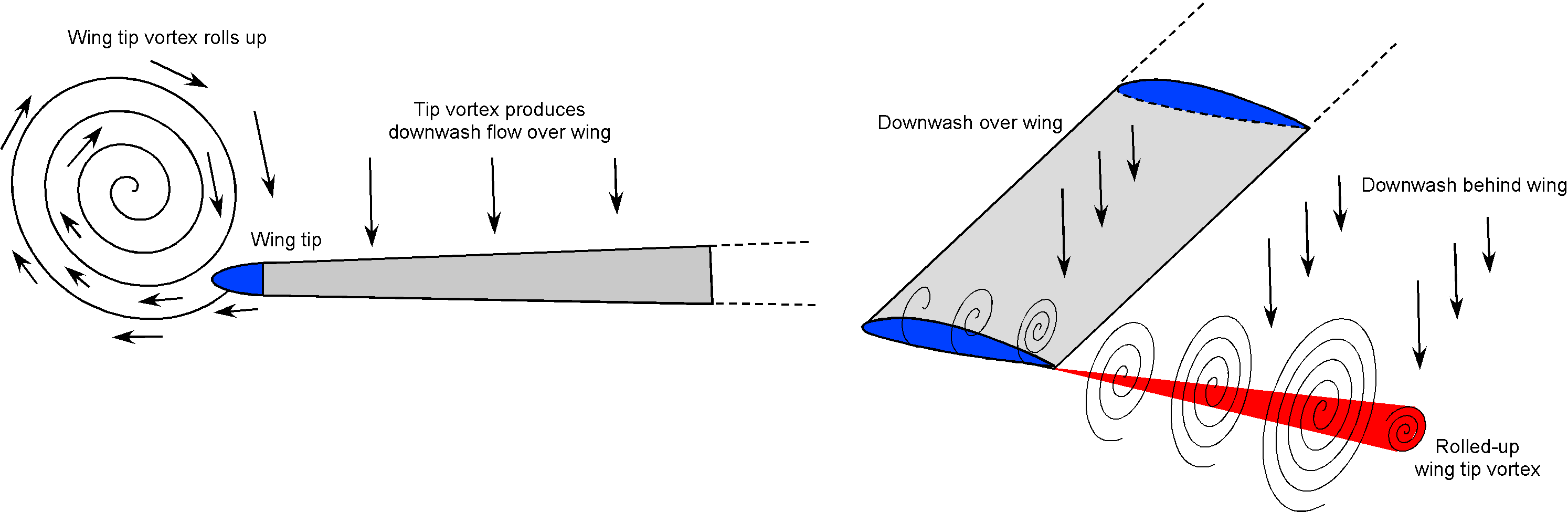
To explain the underlying flow physics of tip vortex formation, it should be remembered that there is a static pressure difference between the upper and lower surfaces, which is the source of the lift on the wing. Research has shown that the tip vortex originates from the tendency of flow to curl around the wing tips under the action of this pressure gradient at the wing tips, as suggested by the schematic below. In this regard, the pressure naturally wants to equalize, so the flow moves in a direction from the higher pressure on the lower surface to the lower pressure on the upper surface. The consequence of this behavior is to initiate a rotational motion in the flow, which is the beginning of the formation of the wing tip vortex.

The wing tip vortices trail from behind the wing, producing a downwash flow over the wing that will reduce its aerodynamic lift and increase its drag.

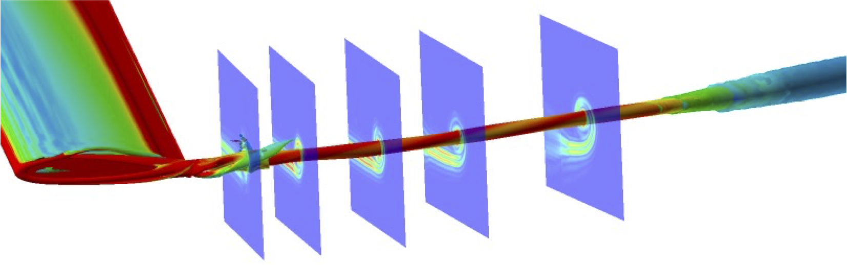
The inherent three-dimensionality of the flow at the wing tip and the tip vortex formation has been researched over many decades, employing experiments and computationally utilizing CFD, an example of the latter being shown below. These results, which can be plotted in terms of flow velocity, pressure, etc., have revealed the complex and intricate aerodynamics of the vortex roll-up. This roll-up process relates to the presence and interaction of three-dimensional boundary layers, flow separation, and shear layers on the wing tip. The tip vortex is usually tightly rolled up within 2 to 3 chord lengths behind the wing. It will then slowly diffuse and spin down under the action of viscosity and turbulence.

The origin of the trailing vortex system from behind a wing is a complex evolutionary process involving the effects of pressure gradients, boundary layers, and flow separation.

One research finding is that the tip vortex formation is an evolutionary process, and it takes some downstream distance before the vortices become fully formed behind a wing. Once they are created, however, they are persistent in that they spin down only slowly under viscosity and turbulence. Another concern is, besides the aerodynamic effects of the vortices on the airplane itself, the possible impact on a following airplane, such as near an airport.

Natural condensation of water vapor over an airplane wing

When an airplane flies, the airflow over the wing causes changes in pressure and temperature. Condensation can occur if the temperature drops sufficiently, leading to visible vapor trails or fogging over the wing. As air flows over the wing, its speed increases, leading to a decrease in pressure according to Bernoulli’s equation, i.e.,

$\frac{1}{2} \varrho V_{\infty}^2 + p_{\infty} = \frac{1}{2} \varrho V^2 + p$

where $\varrho$ is the air density, $V_{\infty}$ is the airspeed, and $V$ is the local flow velocity, with $p_{\infty}$ and $p$ being the corresponding pressures. This pressure drop, $p < p_{\infty}$ , leads to a corresponding drop in temperature. which can be described by the adiabatic relationship

$T = T_{\infty} \left(\frac{p}{p_{\infty}}\right)^{(\gamma-1)/\gamma}$

where $\gamma$ is 1.4 for air. For condensation to occur, the local flow temperature $T$ must be less than or equal to the dew point temperature $T_d$ , i.e., the temperature at which the air becomes saturated. Therefore, the condition for natural condensation effects to occur is

$T_{\infty} \left(\frac{p}{p_0}\right)^{(\gamma-1)/\gamma} \leq T_d$

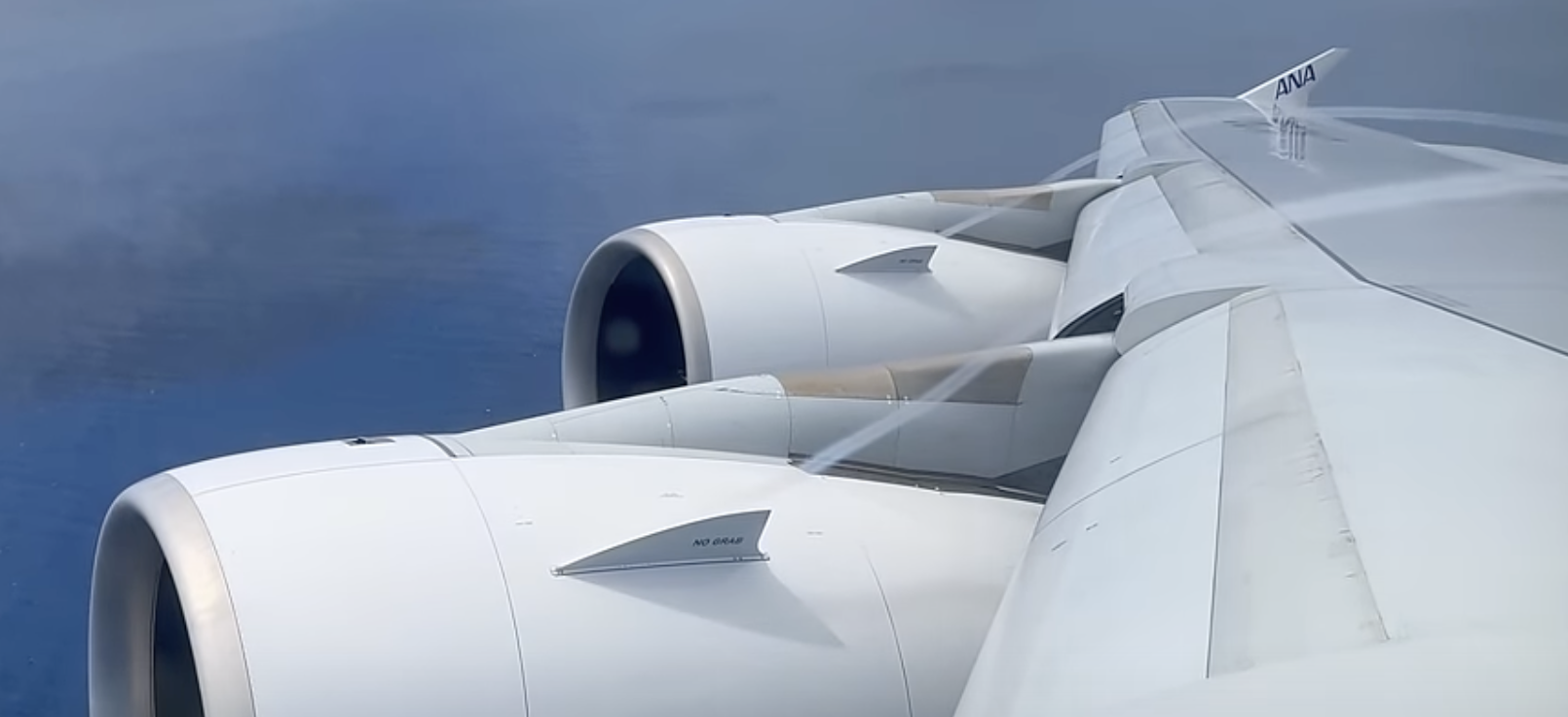
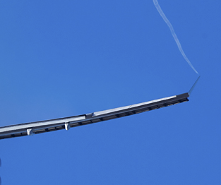
When this condition occurs, typically in humid conditions or near clouds, the flow becomes visible as vapor trails from wing tips, flap side edges, and engine nacelles, an example of the latter being shown in the photo below.

Effects of Trailing Vortices

The induced velocity field from the wingtip vortices is shown in the figure below. Near the center of the vortex, the induced velocity is relatively high. However, the induced velocity decreases inversely with distance from the vortex, so by a semi-span away, the effects diminish significantly. The core region of the wing tip vortex experiences more substantial viscous effects, so it rotates more as a solid body. The core is typically very small, however, of the order of 10% of the wingtip chord.

The induced velocity from a wing tip vortex diminishes inversely with distance from its core.

It will now be apparent that the aerodynamic effects of these rolled-up vortices (one from each wingtip) are significant. First, because of their swirling-induced flow field, they will produce a downwash at each wing section. The principle is shown in the figure below. Adding the downwash flow vector ${w}$ to the free-stream flow vector $V_{\infty}$ produces a resultant flow velocity (or local relative wind) that turns through an angle $\alpha_i$ , called the induced angle of attack. It will be apparent from this figure that the resultant flow now approaches the wing at a different angle and so now creates an “effective” angle of attack, $\alpha_{\rm eff}$ .

The effect of a downwash in the flow ${w}$ is to cause a realignment of the relative wind to the wing section, effectively tilting the lift vector aft to produce a component of drag.

From the geometry of the problem shown above, then the induced angle $\alpha_i$ as given by

(1) $\begin{equation*} \alpha_i = \tan^{-1} \left( \frac{w}{V_{\infty}} \right) \end{equation*}$

which will, in general, be different at each station on the wing, i.e., $w = w(y)$ and $\alpha_i = \alpha_i (y)$ . For small angles, which is typical for a wing, then it is sufficient to write that

(2) $\begin{equation*} \alpha_i = \frac{w}{V_{\infty}} \end{equation*}$

or, in general, that

(3) $\begin{equation*} \alpha_i (y) = \frac{w(y)}{V_{\infty}} \end{equation*}$

Therefore, the effective (and lower) angle of attack of the wing section is now

(4) $\begin{equation*} \alpha_{\rm eff} = \alpha - \alpha_i = \alpha - \left( \dfrac{w}{V_{\infty}} \right) \end{equation*}$

or, in general, that

(5) $\begin{equation*} \alpha_{\rm eff} (y) = \alpha (y) - \alpha_i(y) = \alpha(y) - \left( \dfrac{w(y)}{V_{\infty}} \right) \end{equation*}$

This outcome means that the corresponding lift per unit span will be reduced from its two-dimensional value, i.e., the lift obtained without the effects of the downwash flow. Notice that because ${w}$ will typically be much smaller than $V_{\infty}$ , then the resultant velocity, $V_R$ , can be assumed to be equal to $V_{\infty}$ , i.e.,

(6) $\begin{equation*} V_R = \sqrt{ V_{\infty}^2 + w^2} \approx V_{\infty} \end{equation*}$

It is of particular significance in this situation that the lift vector takes on a new orientation and is tilted slightly rearward from its original direction in two-dimensional flow, thereby reducing the vertical component of the lift. Remember that the lift force, by definition, acts perpendicular to the relative wind, so in this case, it can be seen in the figure above that the lift vector rotates rearward through a slight angle $\alpha_i$ , as does the drag. The consequence is that there is now a component of the lift that acts in the downstream direction, which is called the induced drag, $D'_{i}$ , i.e.,

(7) $\begin{equation*} D'_{i} = L' \, \sin \alpha_i \approx L' \, \alpha_i \end{equation*}$

The induced drag component, $D'_{i}$ , is often called “the drag due to lift” because its origin is primarily a consequence of the formation of the wing tip vortices, and these vortices will only form when the wing creates lift. Therefore, the higher the induced downwash from the wing tip vortices, the higher the induced drag, as illustrated in the figure below.

The induced drag depends on the induced downwash at each wing section.

Remember that $L'$ and $D'_{i}$ represent forces per unit length at each section of the wing, which, in general, will be different, i.e., $L' = L' (y)$ and $D'_{i}= D'_{i}(y)$ . Therefore, the total lift and drag on the wing must be obtained by spanwise integration. Consequently, the total wing lift, $L$ , will be given by

(8) $\begin{equation*} L = \int_{-s}^{s} L' (y) \, dy = 2 \int_{0}^{s} L' (y) \, dy \end{equation*}$

where $y$ varies from $y = -s$ at the left wing tip to $y = s$ at the right wing tip. Similarly, the total induced drag on the wing is given by

(9) $\begin{equation*} D_i = \int_{-s}^{s} D'_{i}(y) \, dy = \int_{-s}^{s} L' (y) \alpha_i (y)\, dy = 2 \int_{0}^{s} L' (y) \alpha_i (y)\, dy \end{equation*}$

Wing Force & Moment Coefficients

When force and moment coefficients are defined for finite wings, a reference length, such as chord length and a reference area, is needed. The reference area is usually the projected or planform wing area, $S$ . The dimensionless coefficients for a finite wing are defined as:

Lift coefficient, $C_{L} = \displaystyle{\frac{L}{q_{\infty} S}} = \displaystyle{\frac{L}{\frac{1}{2} \varrho_{\infty} V_{\infty}^2 \, S}}$

Drag coefficient, $C_{D} = \displaystyle{\frac{D}{q_{\infty} S}} = \displaystyle{\frac{D}{\frac{1}{2} \varrho_{\infty} V_{\infty}^2 \, S}}$

Normal force coefficient, $C_{N} = \displaystyle{\frac{N}{q_{\infty} S}} = \displaystyle{\frac{N}{\frac{1}{2} \varrho_{\infty} V_{\infty}^2 \, S}}$

Axial (chord) force coefficient, $C_{A} = \displaystyle{\frac{A}{q_{\infty} S}} = \displaystyle{\frac{A}{\frac{1}{2} \varrho_{\infty} V_{\infty}^2 \, S}}$

Moment coefficient about some point $a$ , $C_{M_{a}} = \displaystyle{ \frac{M_a}{q_{\infty} \, S \, c_{\rm ref}} } = \displaystyle{ \frac{M_a}{\frac{1}{2} \varrho_{\infty} V_{\infty}^2 \, S \, c_{\rm ref}} }$

Recall that for finite wings, it is generally the convention that the “wing area,” $S$ , is based on the projected planform wing area and not the actual (wetted) surface area. Wing area is obtained by integrating the distribution of wing chord along the span from one wing tip to the other, i.e.,

(10) $\begin{equation*} S = \int_{-s}^{s} c \, dy = \int_{-b/2}^{b/2} c \, dy = 2 \int_{0}^{s} c \, dy = 2 \int_{0}^{b/2} c \, dy \end{equation*}$

where $c = c(y)$ . It is important to distinguish the wing area (symbol capital $S$ ) from the semi-span of the wing (symbol lowercase $s$ ). Notice that the reference area, $S$ , may be defined as the body’s maximum cross-sectional area for bodies such as airplane fuselages or road vehicles. Other than wings, the reference area may not be unique, and standard conventions should always be used when defining force and moment coefficients.

Notice also in these preceding definitions of the coefficients the use of a reference length $c_{\rm ref}$ in the definition of the moment coefficient. For a finite wing, $c_{\rm ref}$ is usually defined as the standard mean chord (SMC) or mean aerodynamic chord (MAC). The SMC is defined as

(11) $\begin{equation*} {\rm SMC} = \overline{c} = \frac{\displaystyle{\int_{-s}^{s} c \, dy}}{b} = \frac{2 \displaystyle{\int_{0}^{s} c \, dy}}{b} = \frac{\displaystyle{\int_{0}^{s} c \, dy}}{s} \end{equation*}$

which, like the wing area, may need to be obtained by spanwise integration. The MAC is

(12) $\begin{equation*} {\rm MAC} = \overline{\overline{c}} = \frac{2 \displaystyle{\int_{0}^{s} c^2 \, dy}}{S} \end{equation*}$

which, like the wing area, may need to be obtained by spanwise integration. Usually $c_{\rm ref} = \overline{\overline{c}}$ , although in some cases $c_{\rm ref} = \overline{c}$ may be used. It is important to note the specific definition being used in any application. For rectangular wings, it will be apparent that $c_{\rm ref} = c = \overline{c} = \overline{\overline{c}}$ .

Measured results for the lift coefficient, $C_L$ , and drag coefficient, $C_D$ , are shown in the figure below for a wing with $A\!R$ = 4. The tests were done at a low Mach number, so the compressibility effects are negligible. Results for two Reynolds numbers of 700,000 and 1,000,000 are shown, which were achieved by varying the flow speed.

Measured lift and drag coefficients for a wing as a function of angle of attack for a NACA 0012 wing.

Check Your Understanding #1 – Finding the lift coefficient of a wing

The wing of a general aviation airplane has a rectangular planform with a span of 30 feet and a chord of 5.25 feet. The airplane has an in-flight weight of 2,105 lb and is cruising at a true airspeed of 120 kts at a pressure altitude of 3,000 ft where the outside air temperature is 72 $^{\circ}$ F. Calculate the lift coefficient of the wing. Assume that all of the lift is carried wing.

Show solution/hide solution.

Because we can assume that lift = weight in level flight, i.e., $L = W$ , then the lift coefficient, $C_{L}$ , is

$C_{L} = \displaystyle{\frac{L}{\frac{1}{2} \varrho_{\infty} V_{\infty}^2 \, S}} = \displaystyle{\frac{W}{\frac{1}{2} \varrho_{\infty} V_{\infty}^2 \, S}}$

Therefore, we need to find the wing area (planform area), $S$ , and the air’s density in which it flies, $\varrho_{\infty}$ . It is a rectangular wing, so the wing area is 30 x 5.25 = 157.5 ft $^2$ . The pressure altitude is 3,000 ft with an outside air temperature of 72 $^{\circ}$ F. ISA standard temperature at 3,000 ft is 57 – 3.57 x 3 = 48.29 $^{\circ}$ F, so 25.71 $^{\circ}$ F warmer than standard. From ISA properties, then $\varrho_{\infty} = 0.0020706$ slug/ft ${^3}$ . We are also given the true airspeed, $V_{\infty}$ , in kts (knots), which needs to be converted to ft/s, i.e., 120 kts = 202.54 ft/s. Therefore, the operating lift coefficient of the wing is

$C_{L} = \displaystyle{\frac{W}{\frac{1}{2} \varrho_{\infty} V_{\infty}^2 \, S}} = \displaystyle{\frac{2,105}{\frac{1}{2} \times 0.0020706 \times 202.54^2 \times 157.5}} = 0.315$

Drag Polar for a Finite Wing

The net effect of these wing tip vortices on the entire wing, therefore, is a reduction in the lift (for a given angle of attack) and an increase in drag, the primary dependency being the effects of wing span and, specifically, the aspect ratio, as shown in the figure below in terms of the drag polar. These classic results, which are wind tunnel measurements from Ludwig Prandtl’s original work on the subject with his students over a century ago, show that the wing’s aspect ratio significantly affects both lift and drag. Recall that the aspect ratio of the wing, $A\!R$ , is defined as the ratio of the square of the wing span to the wing reference area, i.e.,

(13) $\begin{equation*} A\!R = \frac{{\rm span}^2}{\rm area} = \frac{b^2}{S} = \frac{4s^2}{S} = \frac{4s^2}{2 \displaystyle{\int_{0}^{s} c \, dy}} \end{equation*}$

The effects of wing aspect ratio on the drag polar of a finite wing.

The Wright brothers discovered the importance of the aspect ratio!

The Wright brothers noticed the importance of aspect ratio in their wind tunnel experiments in 1900, the results from which were reflected in the design of their “Flier” in 1903. Unlike others at the time, including Lilienthal, Whitehead, and Langley, they understood that the ability to build and fly a high aspect ratio wing was the key to successful flight on their limited engine power. Listen to Professor John Anderson discuss the topic of aspect ratio.

The results in the figure above confirm that the aspect ratio of a wing is critically important in aerodynamic analysis because a higher lift-to-drag ratio can be obtained with wings of a higher aspect ratio, i.e., a long, slender wing with a large span relative to its average chord. The physical reason is that the higher the aspect ratio of the wing, the farther the tip vortices are away from more of the wing. Therefore, their effects produce a lower downwash over the wing and less impact on the three-dimensional aerodynamics.

A reminder of the significance of the drag polar, in this case for a finite wing, is now appropriate because it forms a basis for understanding total airplane performance. An annotated version of a representative polar is shown in the figure below. Notice that the slope of a straight line running from the origin of the graph at (0, 0) to any point on the polar curve is the lift-to-drag ratio of the wing at that operating point.

Representative drag polar for a finite wing. The lift-to-drag ratio is the slope of a straight line running from the graph’s origin at (0, 0) to any point on the polar.

The tangent point of the line to the drag polar represents the highest slope, and so the operating point for the best lift-to-drag ratio, i.e., the best $L/D$ or $C_L/C_D$ , which can be seen to occur at one specific value of the lift coefficient for a given wing as well as its operating Reynolds number and Mach number. The value of $C_{D_{0}}$ represents the part of the drag that is relatively constant and independent of the lift coefficient, i,e., the sum of skin friction and pressure drag or the so-called “parasitic drag, which is sometimes just called “form drag” or “profile drag.”

Calculating the Lift & Drag on a Finite Wing

A finite wing’s lift and induced drag in an ideal “potential” inviscid flow can be calculated using a theoretical formulation known as Prandtl’s lifting line theory. The original formulation assumes an “elliptically loaded” finite wing, which gives, as a consequence, a special case of uniform downwash across the wing span and, therefore, the production of the minimum induced drag. The result for the drag can be expressed in coefficient form as

(14) $\begin{equation*} C_{D_{i}} = \frac{{C_L}^2}{\pi \, A\!R} \end{equation*}$

this much-cited equation shows that the “induced” drag coefficient, $C_{D_{i}}$ , is proportional to the squared value of the lift coefficient of the wing, $C_L$ , and inversely proportional to the aspect ratio of the wing, $A\!R$ . Prandtl’s results, however, as will be described, can also be generalized to a wing with any form of spanwise lift loading.

The lift and drag on a finite wing can also be deduced from using the conservation laws in integral form, which is a more physically tangible result rather than approaching the problem from the lifting line theory. An elliptically spanwise loaded wing with an induced angle of attack $\alpha_i$ produces a flow with a downwash angle $\epsilon = 2 \alpha_i$ in the trailing wake, i.e., there is a vertical change in time rate of change of momentum of the flow as it passes about the wing and turns through an angle $2 \alpha_i$ .

Using these principles, the force on the fluid to increase its vertical momentum can be established, and the reaction force then is the lift on the wing. It is found that the lift on the wing is given by

(15) $\begin{equation*} L = \left[ \varrho_{\infty} \left( \frac{\pi b^2}{2} \right) V_{\infty} \right] V_{\infty} \sin \epsilon \end{equation*}$

Therefore, proceeding using the standard representation of the lift in terms of lift coefficient $C_L$ , then

(16) $\begin{equation*} L = \frac{1}{2} \varrho_{\infty} \, V_{\infty}^2 \, S \, C_L = \varrho \left( \frac{\pi b^2}{4} \right) V_{\infty}^2 \epsilon = \varrho_{\infty} \left( \frac{\pi b^2}{4} \right) \end{equation*}$

Solving for the induced angle of attack of the wing gives

(17) $\begin{equation*} \alpha_i = \frac{C_L}{\pi \, A\!R} \end{equation*}$

The rearward (aft) pointing component of the lift, which is the induced drag $D_i$ , is then obtained from force resolution (assuming small angles), giving

(18) $\begin{equation*} D_i = L \, \alpha_i = L \left( \frac{C_L}{\pi \, A\!R} \right) = \frac{1}{2} \varrho_{\infty} \, V_{\infty}^2 \, S \, C_L \left( \frac{C_L}{\pi \, A\!R} \right) = \frac{1}{2} \varrho_{\infty} V_{\infty}^2 S \left( \frac{{C_L}^2}{\pi \, A\!R} \right) \end{equation*}$

or simply in the coefficient form that

(19) $\begin{equation*} C_{D_{i}} = \frac{{C_L}^2}{\pi \, A\!R} \end{equation*}$

which is another way of deriving Prandtl’s classic formula for the induced drag coefficient of a finite wing with an ideal elliptical spanwise loading.

In the more general case where the wing is not elliptically loaded, then $\alpha_i$ is not the same at all points over the wing. In this case, the induced drag coefficient is given by

(20) $\begin{equation*} C_{D_{i}} = \frac{(1 + \delta) \, {C_L}^2}{\pi \, A\!R} \end{equation*}$

where $\delta > 0$ is known as the wing spanwise efficiency factor, also sometimes known as a span factor.^[1]

The theoretically best aerodynamic efficiency ( $\delta = 0$ ) and lowest induced drag are obtained with a wing planform that is elliptical in planform shape with no twist. This wing shape gives an elliptical spanwise aerodynamic loading (i.e., lift per unit span) and uniform downwash over the wing, which, as previously mentioned, is theoretically the minimum induced drag condition, and so $\delta = 0$ . However, this value is unobtainable in any practical wing design. In practice, values of $\delta$ for a plain wing can range from about 0.01 to 0.1, as shown in the figure below; anything more than 0.1 would usually be classified as a poorly designed wing. However, even a rectangular planform wing will have a reasonably good value of $\delta$ (probably between 0.05 and 0.1) if it has a decent aspect ratio, i.e., $A\!R > 5$ , and also uses some wing twist or washout to control the spanwise lift distribution.

Values of spanwise efficiency factor “ $\delta$ ” factor for several wing planform shapes.

The shape of the wing (i.e., its planform) will affect the distribution of lift and the formation of the trailing vortex system, hence the magnitude of the induced drag on the wing. The idea is to use variations in wing chord along the span and perhaps wing twist and airfoil sections to approximate the ideal elliptical spanwise loading closely and minimize the value of $\delta$ . The actual effective aspect ratio of the wing can also be improved somewhat by paying attention to the shape of the wing tips, which can lower the values of $\delta$ if they are suitably shaped, e.g., with more rounded contours or perhaps with the addition of a winglet.

The photograph below illustrates the nature of the spanwise loading over a wing from the process of natural condensation in the low-pressure zones, which is nominally elliptically distributed, even on this relatively low aspect ratio wing. The highest lift (highest pressure difference) is midspan, and the lowest lift (lowest pressure difference) is at the wing tips. The problem is, however, that even minor deviations from the ideal elliptical form can result in higher induced drag from the wing. Such variations can occur because of interference effects on the wing from the fuselage, engines, undercarriage, external stores, etc.

Natural condensation in the low-pressure area renders visible the nominally elliptical form of the spanwise loading, in this case for an F-15.

Examples of the effects of spanwise interference are shown in the figure below, which are for the same approximate value of total wing lift. Notice that the fuselage can produce significant deviations from the ideal elliptical form, perhaps increasing the value of $\delta$ to over 1.15. However, local effects along the wing, such as because of the aerodynamic interference effects produced by an engine, tend to have more minor effects on the values of $\delta$ .

Flow interference from the effects of the fuselage, engines, etc., tends to spoil the ideal spanwise lift distribution and increase the value of $\delta$ .

Why the effects of the trailing vortices reduce the lift on the wing has already been discussed. Because a result for the induced angle of attack has been obtained, the lift coefficient for a plain finite wing can now be written as

(21) $\begin{equation*} C_L = C_{l_{\alpha}} \alpha_{\rm eff} = C_{l_{\alpha}} \left( \alpha - \alpha_i \right) = C_{l_{\alpha}} \left( \alpha - \frac{(1 + \delta) \, C_L}{\pi \, A\!R } \right) \end{equation*}$

where $C_{l_{\alpha}}$ is the two-dimensional lift-curve slope of the airfoil section that comprises the wing. Rearranging to solve for $C_L$ gives that

(22) $\begin{equation*} C_L = \frac{C_{l_{\alpha}} \alpha}{1 + \displaystyle{\frac{(1 + \delta) \, C_{l_{\alpha}}}{\pi \, A\!R}}} = \left( \frac{C_{l_{\alpha}}}{1 + \displaystyle{\frac{(1 + \delta) \, C_{l_{\alpha}}}{\pi \, A\!R}}}\right) \alpha \end{equation*}$

so the lift-curve slope of the finite wing is reduced to

(23) $\begin{equation*} \frac{d C_L}{d \alpha} = \left( \frac{C_{l_{\alpha}}}{1 + \displaystyle{\frac{(1 + \delta) \ C_{l_{\alpha}}}{\pi \, A\!R}}} \right) \end{equation*}$

The effects are shown in the figure below; the significant reduction of the lift-curve slope with decreasing wing aspect ratio will be apparent.

Results showing the effects of wing aspect ratio on the lift coefficient of a finite wing as a function of its angle of attack.

This preceding result establishes that the lift-curve slope of a finite wing is reduced by decreasing its aspect ratio. It also confirms that in the limiting case where the aspect ratio becomes large and approaches infinity, the lift-curve slope approaches the two-dimensional lift-curve slope of the wing’s airfoil section, i.e.,

(24) $\begin{equation*} \frac{d C_L}{d \alpha} \longrightarrow \frac{d C_l}{d \alpha}~\mbox{\small as $A\!R \rightarrow 0$} \end{equation*}$

Check Your Understanding #2 – Calculating the lift curve slope of a finite wing

Consider a finite wing with an aspect ratio of 7.2 and a spanwise efficiency factor $\delta = 0.1$ . The wing comprises an airfoil with a two-dimensional lift-curve slope of 0.10 per degree. Calculate the lift-curve slope of the finite wing.

Show solution/hide solution.

Notice that a lift-curve slope 0.1 per degree equals $0.1 \times 180/\pi$ = 5.73 per radian angle of attack. The three-dimensional lift-curve slope is calculated using

$\frac{d C_L}{d \alpha} = \left( \frac{C_{l_{\alpha}}}{1 + \displaystyle{ \frac{ ( 1 + \delta) \ C_{l_{\alpha}}}{\pi \, A\!R}}} \right) =\frac{5.73}{1 + \displaystyle{\frac{(1 + 0.1) \times 5.73}{\pi \times 7.2}} } = 5.029\mbox{\small ~/rad} = 0.087\mbox{\small ~/deg}$

Drag Polar for an Airplane

Having developed results for the lift and drag of a finite wing, an approximate result for the drag of an entire airplane can now be established. In the first instance, the best approach is to develop the most straightforward possible representation (i.e., a simple but representative equation) for use in various forms of analysis. The simplest form can be assumed to comprise the sum of the non-lifting and lifting components of drag.

Although there are other lifting surfaces on the airplane, such as the horizontal tail, these contributions can still be included in a single drag contribution so that the drag equation can be represented approximately by

(25) $\begin{equation*} C_D = C_{D_{0}} + \frac{ {C_L}^2}{\pi \, A\!R \, e} = C_{D_{0}} + \left( \frac{1}{\pi \, A\!R \, e} \right) {C_L}^2 = C_{D_{0}} + K {C_L}^2 \end{equation*}$

where $C_{D_{0}}$ is the non-lifting part and $K {C_L}^2$ is the lifting part. This latter equation would be the simplest possible representation of the drag polar for the airplane.

The factor “ $e$ ” is often known as Oswald’s efficiency factor (after William Bailey Oswald), which can be interpreted as the loss of aerodynamic efficiency from non-ideal effects associated with a non-elliptical spanwise lift distribution, as well as the growth in profile drag on the airfoil sections comprising the wing (in aggregate) with increasing ${C_L}^2$ . Indeed, the value of ” $e$ ” can account for the overall airplane’s non-ideal lifting effects in aggregate.

Recall from previously that in the lower angle of attack regime, the profile drag coefficient on an airfoil section can be represented by the equation

(26) $\begin{equation*} C_d = C_{d_{0}} + d_1 \, C_l + d_2 \, {C_l}^2 \end{equation*}$

For a symmetric airfoil (where $\alpha_0 = 0)$ then $d_1$ will be zero. In the case of a finite wing, the net profile drag from the airfoils that comprise the wing can be written as

(27) $\begin{equation*} C_D = C_{D_{0}} + D_1 \, C_L + D_2 \, {C_L}^2 \end{equation*}$

With the addition of the induced drag, the total wing drag becomes

(28) $\begin{equation*} C_D = C_{D_{0}} + D_1 \, C_L + D_2 \, {C_L}^2 + \frac{ (1 + \delta) \, {C_L}^2}{\pi \, A\!R} \end{equation*}$

If $D_1$ is assumed to be zero or small (typical), then

(29) $\begin{equation*} C_D = C_{D_{0}} + D_2 {C_L}^2 + \frac{ (1 + \delta) \, {C_L}^2}{\pi \, A\!R} = C_{D_{0}} + \frac{ {C_L}^2}{\pi \, A\!R \, e} \end{equation*}$

This means that Oswald’s efficiency factor for the wing alone will be given by

(30) $\begin{equation*} e = \frac{1}{\pi \, A\!R \, D_2 + (1+\delta)} \end{equation*}$

and so the representation for $C_D$ as an equation becomes

(31) $\begin{equation*} C_D = C_{D_{0}} + K {C_L}^2 \end{equation*}$

where $K$ is given by

(32) $\begin{equation*} K = \pi \, A\!R \, D_2 + (1 + \delta) \end{equation*}$

In practice, however, other components of the airplane, such as the fuselage and the empennage, can affect the wing aerodynamics, so $K$ is usually higher than that given by this latter equation. Values of $K$ for airplanes typically range from about 1.1 to 1.4, with corresponding values of $e$ varying from about 0.7 (average) to 0.9 (very good). At low angles of attack, such as when the airplane is in cruise, then

(33) $\begin{equation*} e \approx \frac{1}{ 1 + \delta} \end{equation*}$

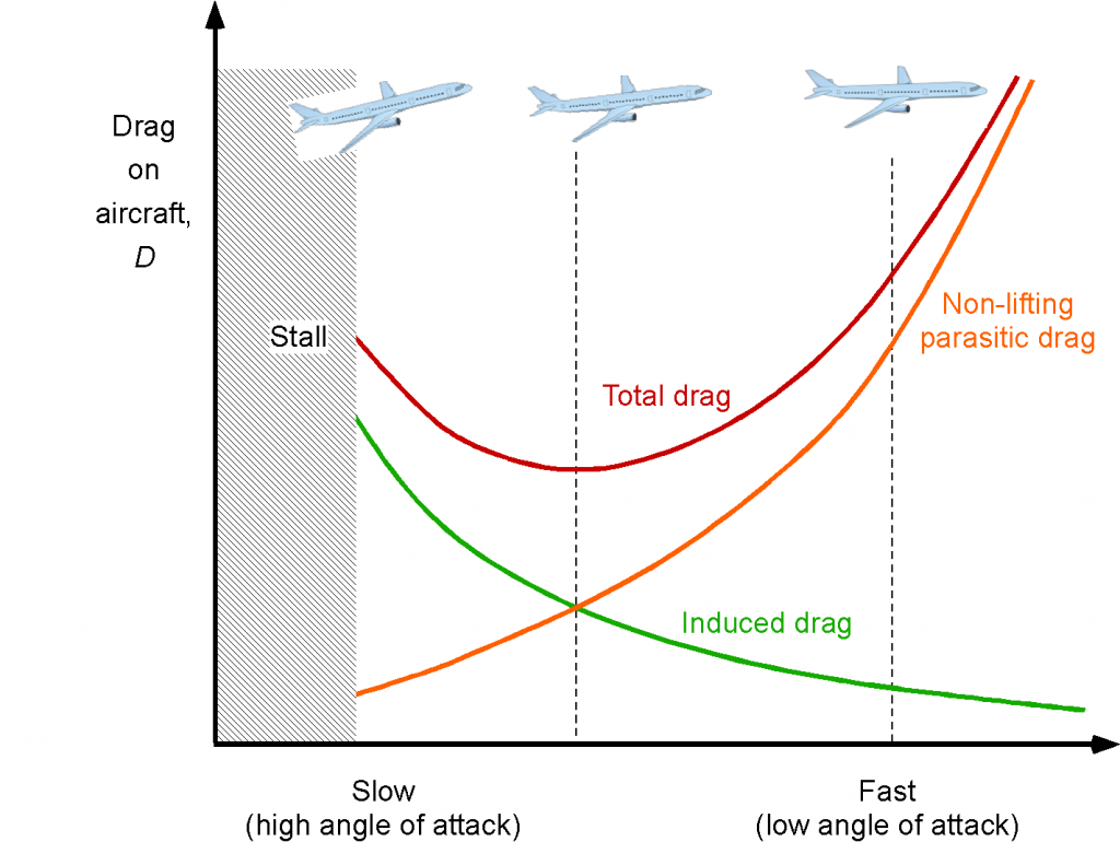
The figure below shows a representative form of the drag polar. The non-lifting part depends primarily on the overall shape of the airplane and is usually called the form drag or parasitic drag coefficient. The lifting part is called the induced drag coefficient or, more generally, “drag due to lift,” and it can be seen that this value depends significantly on the wing’s operating lift coefficient.

The simplest form of a representative drag polar for an airplane comprises a non-lifting part plus a lifting (induced) part.

A table of representative values of $C_{D_{0}}$ and $e$ for several airplanes is shown below. Notice that because of the diversity of airplane designs within one group, it is only possible to give a range of values based on historical data. Such values are helpful in preliminary design studies of new airplanes where the actual values may only be known once more detailed analyses are conducted, including wind tunnel or flight testing.

Representative values of $C_{D_{0}}$ and $e$ based on historical data.
Airplane type	$C_{D_{0}}$	$e$
Twin-engine piston prop	0.022 – 0.028	0.75 – 0.8
Large turboprop	0.018 – 0.024	0.8 – 0.85
GA airplane w/retractable gear	0.02 – 0.03	0.75 – 0.8
GA airplane w/fixed gear	0.025 – 0.04	0.65 – 0.8
Subsonic jet	0.014 – 0.02	0.75 – 0.85
Supersonic jet	0.02 – 0.04	0.6 – 0.8
Sailplane	0.012 – 0.015	0.8 – 0.9
Drones & model aircraft	0.02 – 0.045	0.75 – 0.85

Check Your Understanding #3 – Estimating the non-lifting drag coefficient

The same general aviation airplane is flying under the conditions given in Example #2. Based on engine performance measurements (engine rpm, manifold pressure, engine charts, and propeller efficiency), the propeller is estimated to be producing a thrust of 245 lb to sustain flight. Estimate the non-lifting drag coefficient, $C_{D_{0}}$ , of the aircraft.

Show solution/hide solution.

If the weight of the airplane is 2,105 lb and the thrust required for flight is 245 lb, the lift-to-drag ratio of the airplane is

$\frac{L}{D} = \frac{2,105}{245} = 8.59 = \frac{C_L}{C_D}$

The drag coefficient, $C_{D}$ , is given by

$C_D = \left( \frac{C_D}{C_L} \right) C_L = \frac{0.315}{8.59} = 0.0367$

This latter result can be confirmed using

$C_{D} = \displaystyle{\frac{L}{\frac{1}{2} \varrho_{\infty} V_{\infty}^2 \, S}} = \frac{245}{\frac{1}{2} \times 0.0020706 \times 202.54^2 \times 157.5} = 0.0367$

The classic drag polar for an airplane is

$C_D = C_{D_{0}} + \frac{ (1 + \delta) \, {C_L}^2}{\pi \, A\!R}$

In this case, for a rectangular wing, then $\delta \approx 0.1$ , and the aspect ratio of this particular wing is 30.0/5.25 = 5.71. Therefore,

$C_D = C_{D_{0}} + \frac{ (1 + 0.1) \, {0.315}^2}{\pi \times 5.71} = C_{D_{0}} + 0.00609 = 0.0367$

and so $C_{D_{0}} = 0.030$ , which seems reasonable based on the values for a fixed-gear general aviation airplane as given in the table above.

Thrust Required for Flight

As previously derived, if the simplest form of drag coefficient variation for an airplane is assumed, i.e., using

(34) $\begin{equation*} C_D = C_{D_{0}} + K {C_L}^2 = C_{D_{0}} + \frac{ {C_L}^2}{\pi \, A\!R \, e} \end{equation*}$

The total drag on an airplane can now be calculated as a function of its airspeed. Remember that $A\!R$ is the aspect ratio of the wing, and the value of $e$ (Oswald’s efficiency factor) is always less than unity in any practical case.

Another way of writing this latter equation is

(35) $\begin{equation*} C_D = C_{D_{0}} + C_{D_{i}} \end{equation*}$

where $C_{D_{i}}$ is called the induced drag coefficient or the drag coefficient on the wing resulting from the creation of lift or “lift due to drag,” i.e.,

(36) $\begin{equation*} C_{D_{i}} = \frac{ {C_L}^2}{\pi \, A\!R \, e} \end{equation*}$

The total (dimensional) drag on the airplane is then

(37) $\begin{equation*} D = \frac{1}{2} \varrho V_{\infty}^2 S \left( C_{D_{0}} + \frac{ {C_L}^2}{\pi \, A\!R \, e} \right) \end{equation*}$

which must be equal to the thrust needed from the propulsive system when lift equals weight, i.e., in trimmed, steady, unaccelerated flight, then lift = weight, and thrust = drag, i.e.,

(38) $\begin{equation*} L = W\quad \mbox{\small and} \quad T = D \end{equation*}$

The lift coefficient $C_L$ can be calculated because

(39) $\begin{equation*} L = W = \frac{1}{2} \varrho \, V_{\infty}^2 \, S \, C_L \end{equation*}$

so solving for $C_L$ gives

(40) $\begin{equation*} C_L = \frac{2 W}{\varrho V_{\infty}^2 S} \end{equation*}$

This latter equation shows that for a given wing, then the value of $C_L$ is higher at low airspeeds and lower at higher airspeeds, and $C_L$ also increases with airplane weight. Of course, the maximum attainable lift coefficient is determined by the type of wing, which will reach a point at higher angles of attack when it stalls; the corresponding airspeed is called the stall speed.

Therefore, the drag on the airplane (and hence the thrust required for flight) is

(41) $\begin{equation*} D = T = \frac{1}{2} \varrho_{\infty} V_{\infty}^2 S C_{D_{0}} + \frac{1}{2} \varrho_{\infty} V_{\infty}^2 S \left( \frac{2 W}{\varrho_{\infty} V_{\infty}^2 S} \right)^2 \left( \frac{1}{\pi \, A\!R \, e} \right) \end{equation*}$

and after some rearrangement, then

(42) $\begin{equation*} D = T = \left( \frac{1}{2} \varrho_{\infty} S C_{D_{0}} \right) V_{\infty}^2 + \left( \frac{4 W^2}{\varrho_{\infty} S (\pi \, A\!R \, e)} \right) \frac{1}{V_{\infty}^2 } \end{equation*}$

For a constant weight $W$ and density (altitude), then $\varrho_{\infty}$ , it will be apparent that this equation is of the form

(43) $\begin{equation*} D = T = A V_{\infty}^2 + \frac{B}{V_{\infty}^2} \end{equation*}$

where the values of $A$ and $B$ are now considered to be constants.

This form of the drag variation, and hence the corresponding thrust required for flight, is shown in the figure below. Notice that according to Eq. 43, the profile/parasitic (non-lifting) drag increases with the square of the airspeed, and the induced drag decreases inversely with the square of the airspeed. The resulting drag curve takes on a distinctive “U-shape,” with the minimum drag (and hence thrust required) obtained at some intermediate airspeed.

Representative drag curve for an airplane in level flight has a distinctive U-shape, with a minimum drag at an intermediate airspeed. After reaching this minimum point, the drag grows quickly with increasing airspeed.

The corresponding power required for flight is

(44) $\begin{equation*} P_{\rm req} = T V_{\infty} \end{equation*}$

which is of the form

(45) $\begin{equation*} P= A V_{\infty}^3 + \frac{B}{V_{\infty}} \end{equation*}$

As airspeed increases, more power (and hence more fuel) is required for flight because power increases with the cube of airspeed.

Check Your Understanding #4 – Calculating the drag on a finite wing

Consider a flying wing with a wing area of 210 m², an aspect ratio of 10, and an Oswald’s efficiency factor of 0.90. The airfoil section on the wing has a profile drag coefficient of 0.015. The mass of the airplane is 50,000 kg. If the airplane is flying at a density altitude of 3 km and the true airspeed is 230 m/s, then calculate the total drag on the airplane.

Show solution/hide solution.

The air density at a density altitude of 3 km is 0.90925 kg m^-3 when using the ISA model. For vertical force equilibrium, the lift on the wing $L$ is equal to the weight of the airplane, $W$ , i.e.,

$L = M g = 50,000 \times 9.81 =490,500 {\mbox N}$

The lift is given by

$L = \frac{1}{2} \varrho V^2 S C_L$

so the operating lift coefficient of the wing is

$C_L = \frac{L}{ \frac{1}{2} \varrho V^2 S}$

Inserting the known values gives

$C_L = \frac{490,500 }{0.5 \times 0.90925 \times 230.0^2 \times 210.0} = 0.097$

The drag coefficient is

$C_D = C_{D_{0}} + \frac{{C_L}^2}{\pi \, A\!R \, e} = 0.015 + \frac{0.097^2}{\pi \times 10.0 \times 0.90} = 0.0153$

where the non-lifting part $C_{D_{0}} = 0.015$ , i.e., $C_{D_{0}} = C_{d_{0}}$ . Therefore, the total drag force is

$D = \frac{1}{2} \varrho V^2 S C_D = 0.5 \times 0.90925 \times 230.0^2 \times 210.0 \times 0.0153 = 77,271.6~\mbox{ N}$

which gives a corresponding lift-to-drag ratio of about 6.

Generalization of the Airplane Drag Polar

The drag produced on an airplane will also be a function of the Reynolds number and flight Mach number. Therefore, another generalization of the prior approach is to write that

(46) $\begin{equation*} C_D = C_{D_{0}}(Re, M_{\infty}) + D_1 (Re, M_{\infty}) C_L + D_2 (Re, M_{\infty}) {C_L}^2 \end{equation*}$

although, again, the challenge is evaluating the values of the coefficients; this will usually involve a combination of wind tunnel measurements and flight tests.

Usually, for higher Mach numbers above 0.3, the effects of Mach number on the aerodynamics are more important than the effects of Reynolds number so that Reynolds number variations can be ignored, i.e.,

(47) $\begin{equation*} C_D = C_{D_{0}}(M_{\infty}) + D_1 (M_{\infty}) \, C_L + D_2 (M_{\infty}) \, {C_L}^2 \end{equation*}$

Finally, these forgoing equations will apply to an airplane where the minimum drag is obtained at zero lift conditions. If this is not the case, then a further generalization is to use

(48) $\begin{equation*} C_D = C_{D_{\rm min}} + K \left( C_L - C_{L_{\rm min~drag}} \right)^2 \end{equation*}$

as shown in the figure below.

Generalization of the drag polar for an airplane. This form is usually more appropriate for flight at higher subsonic flight Mach numbers.

Winglets

The purpose of winglets is to increase the effective aspect ratio of the wing but without significantly increasing the wing’s span. The classic “Whitcomb” winglet moves the tip vortices from the wing tip to the top of the winglet, as confirmed in the photograph below. The consequence is that the tip vortices are further away from more of the wing, reducing the magnitude of the induced downwash all over the wing and decreasing its induced drag. The flow velocities induced by the tip vortices decrease inversely with distance, so even a small winglet can decrease the downwash velocities over the wing, measurably reducing drag.

Confirmation that a “tip vortex” forms at the tip of a winglet, which is rendered visible by natural condensation.

Today, airplanes have a winglet by design or are retrofitted with winglets after delivery. The motivation is evident in that a winglet can reduce drag and save fuel. While the winglet adds some structural weight and produces a small increment in skin friction drag, the reductions in induced drag outweigh these concerns. Fuel savings can offset the cost of retrofitting a winglet to an airliner in as little as two years. Therefore, using a winglet makes sense compared to a wing redesign with a higher wing span and aspect ratio.

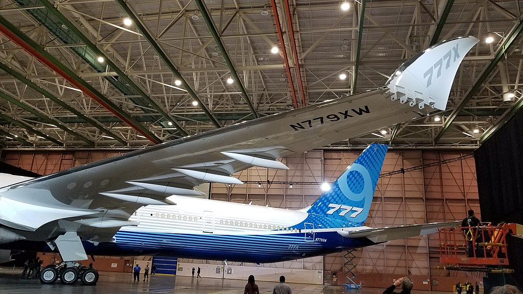
A large “Jumbo” airliner’s feasible wingspan and aspect ratio may be limited for several reasons, such as higher wing weight and the possibility of aeroelastic issues. Airport operations, such as taxiway access, parking, hangar size, etc., also impose factors. The Boeing 777X is unique because of its extremely high wingspan and aspect ratio, it uses a folding wing tip design. The idea is to give an ultra-high aspect ratio wing for flight while having a reduced wing span on the ground; in this regard, a winglet to boost the wing’s effective aspect ratio is unnecessary.

The Boeing 777X has no winglets but an ultra-high aspect ratio wing. The extra-long wing span requires the wingtips to be folded to allow safe ground operations.

There are no validated theoretical formulas that can be used to calculate the effects of winglets, but one common approach is to use an aspect ratio correction of the form

(49) $\begin{equation*} A\!R_{\rm eff} = A\!R \left( 1 + K_{\rm wl} \, \frac{h_{\rm wl}}{s} \right) \end{equation*}$

where $A\!R_{\rm eff}$ is the “effective” or corrected aspect ratio, $h_{\rm wl}$ is the length or height of the winglet, as shown in the figure below, and $K_{\rm}$ is an empirical coefficient that depends on the type of winglet.

Winglets increase the effective aspect ratio and reduce the induced drag.

For a classic Whitcomb winglet, it is usually assumed in Eq. 49 that $K_{\rm wl} = 0.95$ , at least for preliminary design or airplane performance estimates. The lifting or induced component of the drag can then be written as

(50) $\begin{equation*} C_{D_{i}} = \frac{ {C_L}^2}{\pi \, AR_{\rm eff} \, e} \end{equation*}$

While winglets present some additional surface area to the flow and somewhat increase the profile (non-lifting) drag, the benefits are realized over the range of lift coefficients during flight, as shown in the figure below. Lift-to-drag curves for airplanes tend to be quite “peaky,” although the range of lift coefficients at which the highest lift-to-drag ratios can be maintained and even widened by sedulous airfoil and wing design. In this regard, the ability to maintain aerodynamic efficiency over a broader range of airspeeds, weights, and altitudes can be realized.

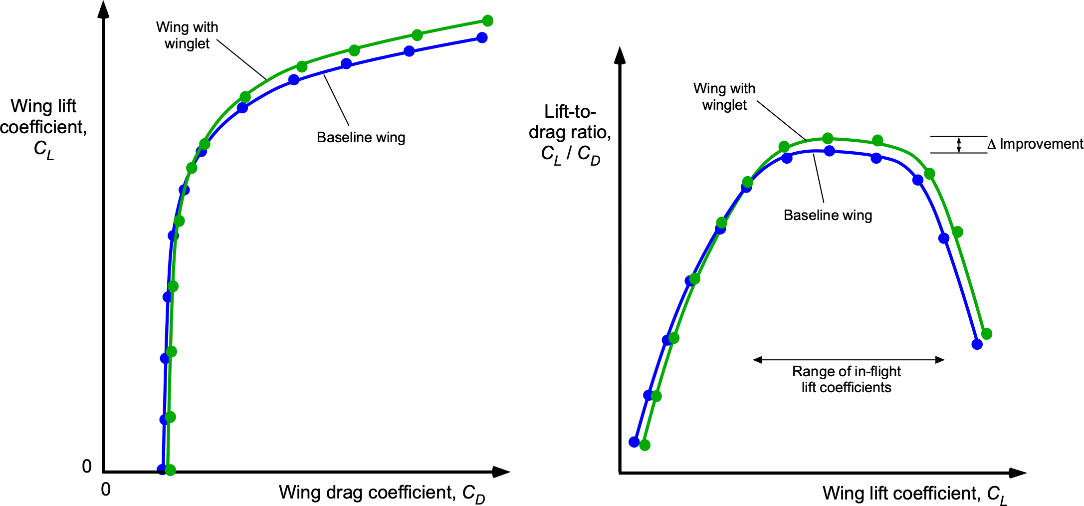
The improvements in the lift-to-drag ratio obtained using a winglet may be small but fuel savings over the life of the airplane can be significant.

While the increase in lift-to-drag ratio using a winglet may only be a few percent relative to a baseline wing, the reductions in thrust required for a given airspeed can translate into substantial reductions in fuel burn during each flight. The actual fuel savings will depend on the airplane type, the flight length, and the typical operating conditions. However, studies and industry data have shown that winglets can provide significant fuel savings. For example, a Boeing 737 equipped with blended winglets has been reported to achieve an average fuel savings of around 4% compared to the same airplane without winglets. Similarly, certain Airbus airplanes fitted with blended winglets, such as the A350, have shown fuel savings from 3% to 4%. The upshot then is that winglets can measuraby extend the flight range of an airliner and/or increase its payload capacity.

While these performance benefits and resulting fuel savings might seem relatively modest, considering the high fuel consumption of commercial airliners and the large number of flights they operate, even a slight percentage improvement in fuel efficiency can result in significant cost savings for airlines. Over the life of a commercial jetliner, which can exceed 25 years, the fuel savings can translate into millions of dollars for just one airplane. Therefore, fuel savings for a fleet of airliners in just one airline can reach into the tens or even hundreds of millions of dollars.

Effects of Compressibility & Wing Sweep

One issue that must be remembered is that a wing’s drag increases quickly as the flight Mach number approaches transonic conditions, a result of the development of shock waves and wave drag. However, such effects are difficult to generalize because the drag depends critically on the specific wing geometry (especially its thickness and sweepback angle) and operating lift coefficient.

The figures below show representative wind tunnel measurements of the minimum (non-lifting) drag on semi-span wings with different sweepback angles, $\Lambda$ , and different thickness-to-chord ratios, $t/c$ . The transonic and supersonic drag will be minimized for a given sweepback by using as thin a wing as possible, bearing in mind that this may not be possible in practice for structural reasons. However, even with a thin wing, significant benefits can still be realized by using sweepback, especially in the supersonic regime.

The effects of thickness sweepback angle on the non-lifting drag of a semi-span wing in transonic and supersonic flow.

The effects of thickness-to-chord ratio on the non-lifting drag of a semi-span wing in transonic and supersonic flow.

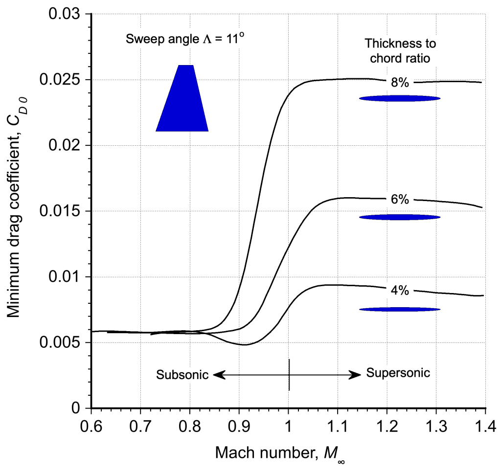
An approximate equation to quantify the increment to the drag to account for the formation of shock waves and the associated wave drag is called “Lock’s fourth power rule.” The original work was published in the report: “The Ideal Drag Due to a Shock Wave Parts I and II,” ARC report 2512 (1951) by C. N. H. Lock,” and the primary process has seen refinements and other developments by engineers over the years.

The Lock model requires a value of the critical Mach number of the wing, $M_{\rm crit}$ , which is the flight Mach number at which the onset of supersonic flow first appears. Lock first argued that the drag of a shock wave per length (or its height extending from the surface of the wing) scales proportionally with the third power of the value of the flight Mach number above the critical Mach number, i.e., with $(M_{\infty} - M_{\rm crit})^3$ . Second, Lock argued that the height of the shock wave is also proportional to $M_{\infty} - M_{\rm crit}$ . The net result is a wave drag increment proportional to the fourth power, i.e., $(M_{\infty} - M_{\rm crit})^4$ . A constant $k_w$ also appears in the final expression for the wave drag increment, $\Delta C_{D_{w}}$ , i.e.,

(51) $\begin{equation*} \Delta C_{D_{w}} = k_w \left( M_{\infty} - M_{\rm crit} \right)^4 \end{equation*}$

which is valid for $M_{\infty} \ge M_{\rm crit}$ .

Therefore, including the wave drag increment, the drag equation for the airplane can be written as

(52) $\begin{equation*} C_D = C_{D_{0}} + D_1 \, C_L + D_2 \, {C_L}^2 + k_w \left( M_{\infty} - M_{\rm crit} \right)^4 \end{equation*}$

where $C_{D_{0}}$ , $D_1$ , and $D_2$ are all functions of Mach number. While the Lock equation has been found to give reasonably good predictions of the extra wave drag, quantitative predictions for specific airplanes depend on the value of $k_w$ . Without any other information, a value $k_w = 20$ is often used for the preliminary design of an airplane, such as an airliner designed to cruise in transonic flight where $0.7 \le M_{\rm crit} \le 0.8$ . For airplanes with thin, supersonic airfoils with higher critical Mach numbers, $k_w = 5$ is appropriate.

Examples of Airplane Drag Polars

A combination of calculations (maybe even with CFD), wind tunnel measurements, and flight tests can define the drag polar to an acceptable degree of fidelity for performance evaluations and other applications. Drag polars have been published for various airplanes, including general aviation airplanes, gliders, commercial airplanes, and military airplanes. One purpose of publishing such results is to allow engineers and analysts to validate their modeling and use it for instructional purposes.

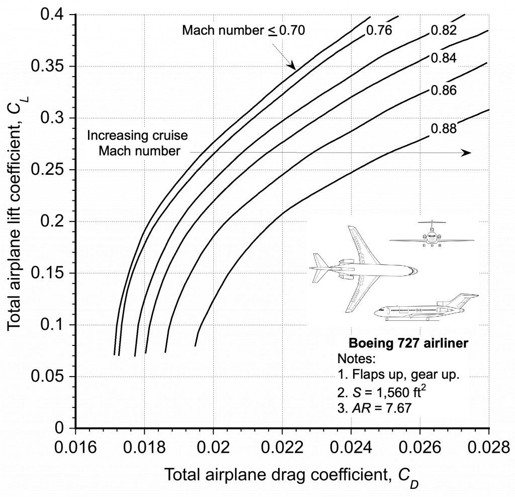
An example of a complete drag polar for a legacy commercial airplane, shown in the figure below, at higher subsonic Mach numbers and into the transonic domain. First, notice the increase in the zero-lift drag coefficient $C_{D_{0}}$ with increasing Mach number. Second, notice the more rapid growth in the drag as transonic conditions are approached and established (i.e., for $M_{\infty} > 0.76$ ), this being the consequence of exceeding the critical Mach number and the development of shock waves and a commensurate increase in wave drag.

Drag polars for a commercial airplane at subsonic and transonic flight Mach numbers.

Another example of a drag polar is for a legacy military fighter airplane, shown below. In this case, the results are for subsonic and transonic flight, as well as for supersonic flight. Again, the rapid increase in drag is apparent as transonic conditions are encountered and supersonic flight is approached. Notice that the airplane has a lift-to-drag ratio of only about 3 in supersonic flight. For a military airplane, it is the usual practice to determine another form of the drag polar as a function of the load factor, i.e., for maneuvering flight.

Drag polars for a military fighter airplane for subsonic, transonic and supersonic flight Mach numbers.

Check Your Understanding #5 – Finding the lift-to-drag ratio of a wing

The drag coefficient $C_D$ of a particular airplane design is described by the equation

$C_D = 0.04 + \left( \frac{1.26}{\pi \, A\!R} \right) {C_L}^2$

where $A\!R$ is the aspect ratio of the wing. For aspect ratios of 10 and 20, determine the best lift-to-drag ratio of the wing and the lift coefficient at which this occurs.

Show solution/hide solution.

The drag coefficient for the airplane is given by

$C_D = 0.04 + \left( \frac{1.26}{\pi \, A\!R} \right) {C_L}^2 = A + B {C_L}^2$

This means that

$\frac{C_D}{C_L} = \frac{A}{C_L} + B C_L$

Differentiating the preceding expression gives

$\frac{d (C_D/C_L)}{C_L} = -\frac{A}{{C_L}^2} + B = 0 \mbox{\small ~~for a maximum or minimum}$

Therefore, solving for $C_L$ at this condition gives

$C_L = \sqrt{ \frac{A}{B} } = \sqrt{ \frac{0.04 \pi \, A\!R}{1.26} }$

This will be the lift coefficient used to obtain the maximum lift-to-drag ratio for a wing with a given aspect ratio.

For $A\!R = 10$ then the $C_L$ for best $C_L/C_D$ is

$C_L = \sqrt{ \frac{0.04 \pi \, A\!R}{1.26} } = \sqrt{ \frac{0.04 \times \pi \times 10 }{1.26} } = 1.0$

and substituting values with $C_L$ = 1.0 gives the best lift-to-drag ratio as

$\frac{C_L}{C_D} = \frac{C_L}{0.04 + (1.26/\pi/AR){C_L}^2} = \frac{1.0}{0.04 + (1.26/\pi/10) 1.0^2} = 12.48$

For $A\!R = 20$ then the $C_L$ for best $C_L/C_D$ is

$C_L = \sqrt{ \frac{0.04 \pi \, A\!R}{1.26} } = \sqrt{ \frac{0.04 \times \pi \times 20 }{1.26} } = 1.41$

and substituting values with $C_L$ = 1.41 gives the best lift-to-drag ratio as

$\frac{C_L}{C_D} = \frac{C_L}{0.04 + (1.26/\pi/AR){C_L}^2} = \frac{1.41}{0.04+ (1.26/\pi/20) 1.41^2} = 17.65$

Center of Pressure & Aerodynamic Center

The procedures for finding the center of pressure and aerodynamic center on a finite wing are similar to those for two-dimensional airfoils. Recall that, by definition, the center of pressure on a wing is a point about which the pitching moments are zero, i.e., a point where the resultant forces can be assumed to act. The aerodynamic center is a point where the moment is constant and independent of the angle of attack. Determining the aerodynamic center, like that for the center of pressure, requires values of the lift and moment coefficient versus the angle of attack about any other point, which by default is usually the 1/4-chord.

In the case of the center of pressure, then

(53) $\begin{equation*} \frac{x_{\rm cp}}{c} = \frac{1}{4} - \frac{C_{M_{c/4}}}{C_{L}} \end{equation*}$

Because the center of pressure is a moving point, the center of pressure to resolve the forces and moments on a wing is not used much in practice.

If the aerodynamic center is assumed to be at a distance $x_{ac}$ behind the leading edge, then

(54) $\begin{equation*} C_{M_{a}} = C_{M_{\rm ac}} - C_{L} \left( \frac{x_{ac}}{c} - \frac{a}{c} \right) \end{equation*}$

Differentiating the above equation with respect to $C_{L}$ gives

(55) $\begin{equation*} \frac{d C_{M_{a}}}{dC_{L}} = \frac{d C_{M_{\rm ac}}}{dC_{L}} - \left( \frac{x_{\rm ac}}{c} - \frac{a}{c} \right) \end{equation*}$

After rearrangement then

(56) $\begin{equation*} \frac{x_{\rm ac}}{c} = \frac{a}{c} - \frac{d C_{M_{a}}}{dC_{L}} \end{equation*}$

The value of $dC_{M_{\alpha}}/d C_L$ can be obtained by using

(57) $\begin{equation*} \frac{d C_{M_{\alpha}} }{ d C_L} = \left( \frac{ d C_{M_{\alpha}}}{d \alpha}\right) \left( \frac{d \alpha}{d C_{L}}\right) \end{equation*}$

This latter process is performed by finding the slopes of the best straight line fit to the values on the graphs of $C_L$ versus the angle of attack of the wing $\alpha$ and also the $C_{M_{1/4}}$ curve versus $\alpha$ .

Vortex Wake Upsets

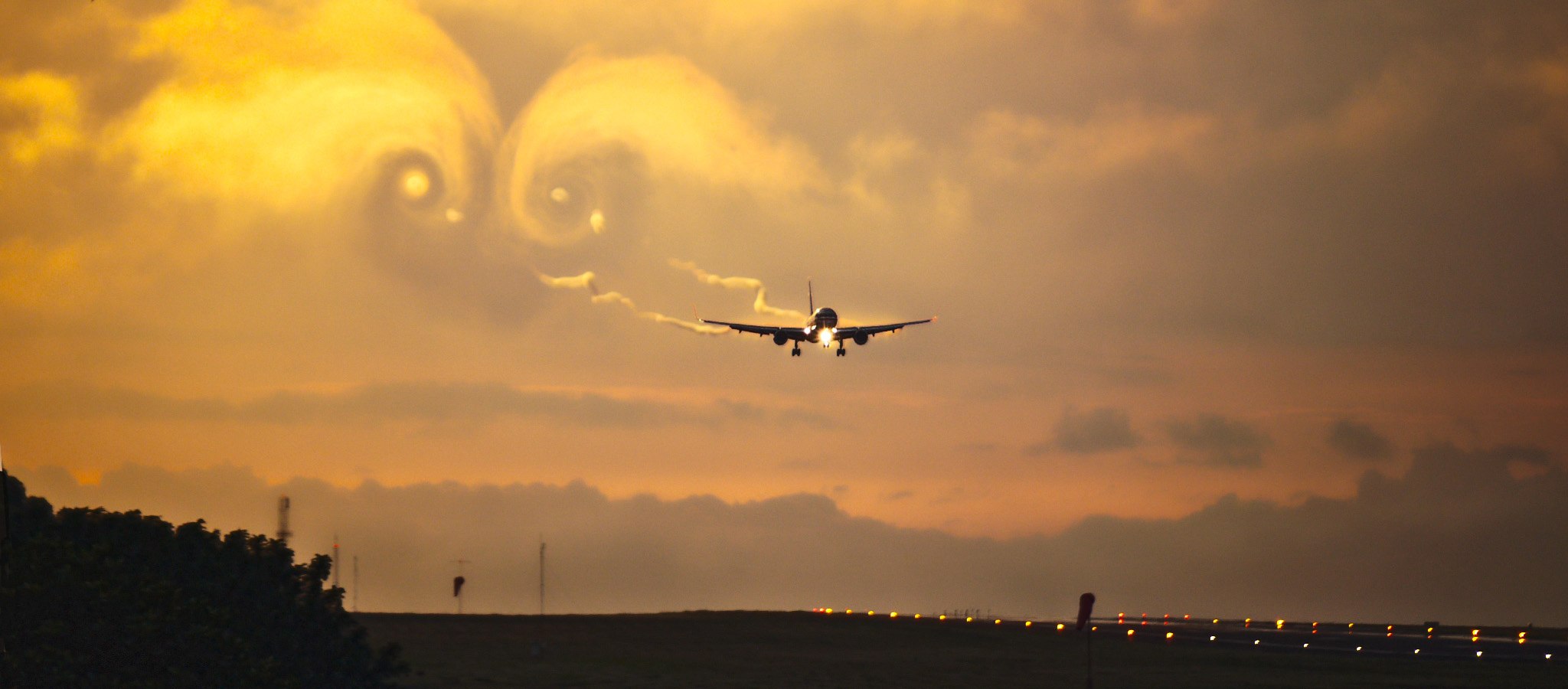
When viewed from in front of the airplane, the tip vortex from the left wing tip rotates counterclockwise and the right one clockwise, as the photograph below suggests. The vortices tend to be the strongest when the wing operates at high angles of attack, such as during takeoff and landing. As the tip vortices trail back from the wing tips, they descend behind the wing under their self-induced velocities.

Natural flow visualization of the wake behind a landing airplane, showing the signature of the wing tip vortices left in the cloud patterns.

While the wing tip vortices affect the airplane that generates them, a concern over the persistence of these vortices is their possible effects on the following airplane. The generic name used for the impact of the vortex wake, especially by pilots and the FAA, is called wake turbulence. Wing tip vortices tend to be relatively strong and persistent and can remain for up to several minutes and many miles after the passage of an airplane through a given part of the sky. The persistence of the vortices also depends on the winds and other environmental factors, such as atmospheric turbulence.

Because the wing tip vortices persist and can take many minutes to spin down, they can pose a concern for the following airplane, particularly in the terminal area. In addition, the local downwash velocities may be a significant fraction of the airplane’s airspeed with steep downwash gradients, so the potential hazard is significant in that it will affect the angle of attack and, thus, the lift on the wing.

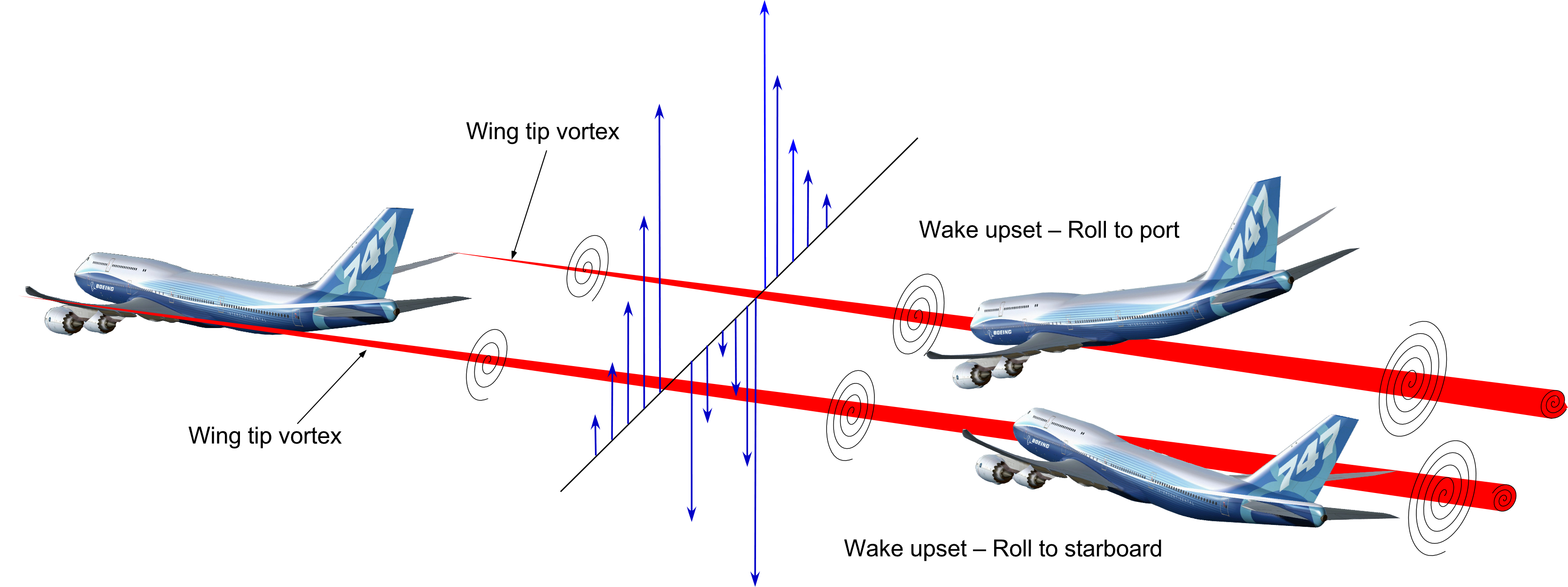
Notice from the figure below that an airplane may end up flying more perpendicularly or parallel to the wing tip vortices. On the one hand, flying nearly perpendicular to the vortices will cause the airplane to encounter an abrupt upwash followed by a downwash and then another upwash. This trajectory can cause notable changes in the airplane’s load factor when flying through it and may concern the passengers, who may feel a very distinct “bump.” On the other hand, if an airplane flies parallel to the vortices, there is a tendency for the airplane to roll, which is a bad outcome. Hence the name vortex wake upsets becomes clear.

Because of the persistence of the wing tip vortices they can pose a concern for the following airplane, particularly in the terminal area.

The possibility and problems of wake upsets during takeoff and landing operations became much more acute starting in the 1970s with the introduction of wide-body or jumbo jets such as the Boeing 747 and McDonnell-Douglas DC-10. The higher weights of these airplanes produced intense and persistent wing tip vortices that caused many “wake turbulence” incidents. The most prevalent were for smaller airplanes, which caused them to roll inverted in some cases of wake encounters.

Subsequently, the FAA has mandated much greater horizontal separation distances between all aircraft in the terminal airspace regions, thereby dramatically reducing the upsets from wake turbulence. However, increasing separation distances between aircraft limits the number of aircraft that can land and take off within a given time, which can seriously constrain aircraft movements at busy airports.

Summary & Closure

The aerodynamics of wings of finite span depend critically on their aspect ratio. The higher the aspect ratio, the lower the induced component of the drag. Induced drag is an inevitable consequence of lift generation and is highest when the wing operates at higher lift coefficients, thereby creating the strongest wing tip vortices. These vortices produce a downwash flow velocity over the wing, altering the lift and drag at every wing section. Therefore, the design of finite wings for minimum drag also depends on the spanwise lift distribution, which should be as close to elliptical as possible and can be achieved by judicious variations in planform (local wing chord), wing twist, and airfoil section.

5-Question Self-Assessment Quickquiz

For Further Thought or Discussion

Calculate the potential improvement in lift-to-drag ratio for a wing when making a design change in the aspect ratio from 5 to 7 while keeping the same wing area. Make any reasonable assumptions.
It said that a winglet increases the wing’s effective aspect ratio without an increase in its span. Discuss why.
The drag polar for a high-speed airplane shows a general reduction in the slope of the curves when approaching and exceeding Mach 1. Discuss why this behavior occurs.
Why does the aspect ratio of a wing become less important at supersonic speeds?
Mandating greater separation distances between all aircraft in terminal airspace has reduced the likelihood of wake upsets but has led to other problems. Discuss.

Other Useful Online Resources

To understand more about the aerodynamics of finite wings then, explore some of these online resources:

Listen to Professor John Anderson discuss: The Wright Brothers Discover Aspect Ratio.
Great educational film on: The Secret of Flight 8: The Induced Drag.
To see more on vortex wake-induced drag, check out this animation and explainer.
Read an interesting journal paper on the measurement of vortex wakes.
A YouTube video showing aircraft wakes from natural condensation effects.

In the Prandtl lifting-line theory, the values of $\delta$ can be calculated by assuming that the spanwise loading over the wing comprises a series of "modes" expressed as a Fourier series. ↵

License

Icon for the Creative Commons Attribution-NonCommercial-NoDerivatives 4.0 International License

Introduction to Aerospace Flight Vehicles Copyright © 2022–2025 by J. Gordon Leishman is licensed under a Creative Commons Attribution-NonCommercial-NoDerivatives 4.0 International License, except where otherwise noted.

Digital Object Identifier (DOI)

https://doi.org/https://doi.org/10.15394/eaglepub.2022.1066.n24