46 Steady Level-Flight Operations
Introduction
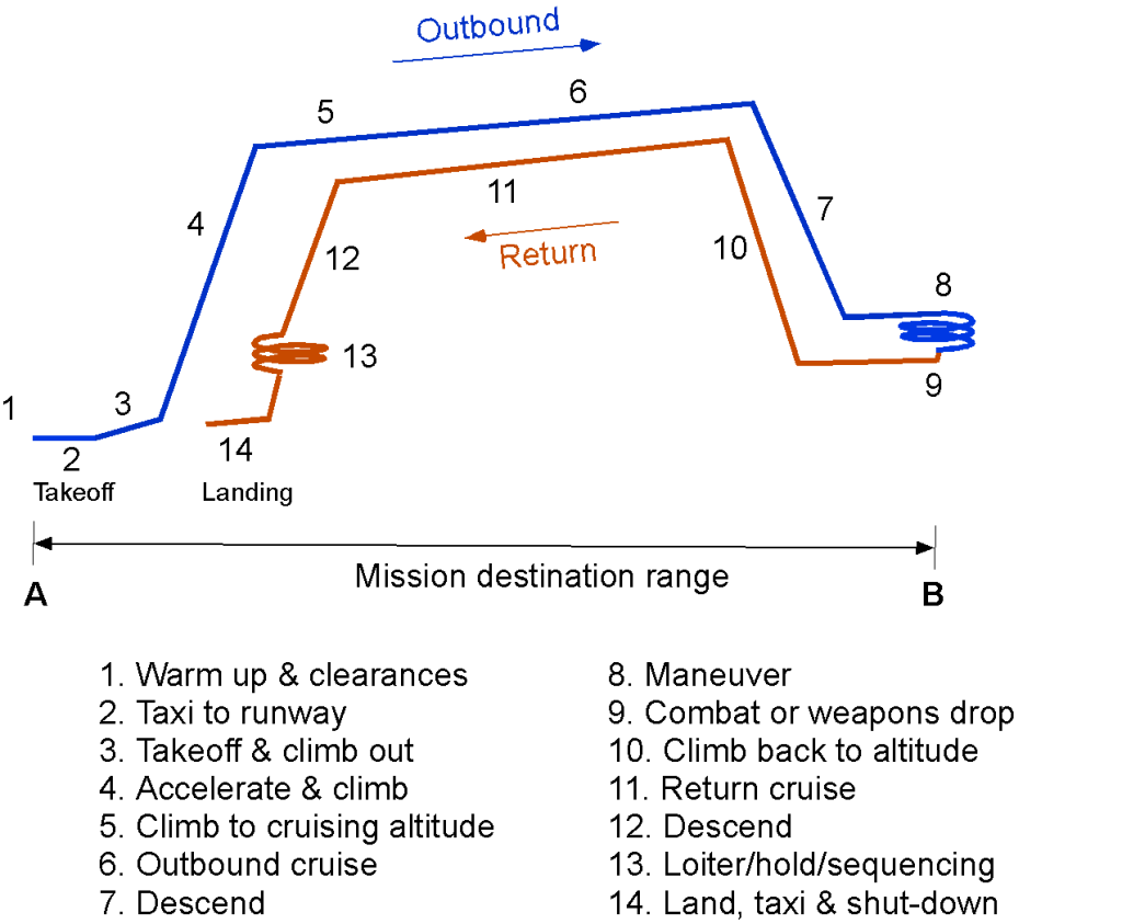
An airplane’s typical operation involves several phases of flight, including takeoff, climb, cruise, turns or maneuvers, descent, and landing. As shown in the figure below, a civil aircraft, such as a commercial airliner, spends a significant portion of its flight time in cruise conditions, flying from one airport to another. This condition is predominantly in straight and level, unaccelerated flight at relatively constant airspeed and high altitudes. A contingency plan for a possible diversion because of adverse weather conditions or other issues at the destination, which could prevent landing, must always be accounted for, requiring reserve fuel to be carried. Reserve fuel is extra weight, so from a performance perspective, it costs fuel to carry fuel.

A military aircraft may spend much more of its flight time conducting climbs, turns, and maneuvers, and the cruise segment may be much shorter. The mission may also involve an out-and-return mission profile, i.e., flying to a destination to conduct some operation and returning to base without landing, as shown below. However, the mission may also involve additional stops en route before returning to base. Such missions are commonly known in operational contexts as round-robin missions. Nevertheless, understanding an airplane’s steady-level flight performance is essential for determining its flight range at normal cruising speeds, operational altitudes, ceilings, and airspeeds to attain maximum flight range and endurance.
The analysis of level flight performance depends critically on the type of propulsion system and its characteristics, specifically whether the aircraft is jet-propelled or propeller-driven. Accordingly, engines are commonly classified into two broad categories: engines driving propellers (such as piston engines and turboprops) and jet engines (including turbojets and turbofans). The primary consideration in analyzing airplane flight performance is that the output of a jet engine is quantifiable in terms of its thrust production. In contrast, the output of an engine driving a propeller is quantifiable in terms of its shaft power output.
However, it must also be recognized that engines driving propellers convert their power into propulsive thrust through the aerodynamics of the propeller, which will have its own specific performance characteristics. For jet engines, power is required to produce thrust by increasing the momentum of the flow through the engine; both mass flow rate and jet velocity contribute to the thrust. Therefore, all engines are examined as power-producing devices, so they are generally referred to as powerplants. Another reason is that they generate electrical, hydraulic, and pneumatic power, in addition to thrust or propulsive power. Additionally, recognize that fuel is required to produce power; therefore, for airplane performance, the fuel flow and, hence, the fuel burned during flight, are always at the core of the analysis.
Learning Objectives
- Be aware of an airplane’s general performance characteristics in straight and level flight.
- Understand the fundamental differences between the performance analyses of jet-powered and propeller-driven aircraft.
- Review typical thrust-required curves for jet-powered aircraft and power-required curves for propeller-driven aircraft.
- Appreciate the effects of weight and altitude on thrust required and/or power required performance curves and flight characteristics.
- Learn how to use the equivalent weight method to derive airplane performance parameters from flight-test data.
Performance Characteristics of an Airplane
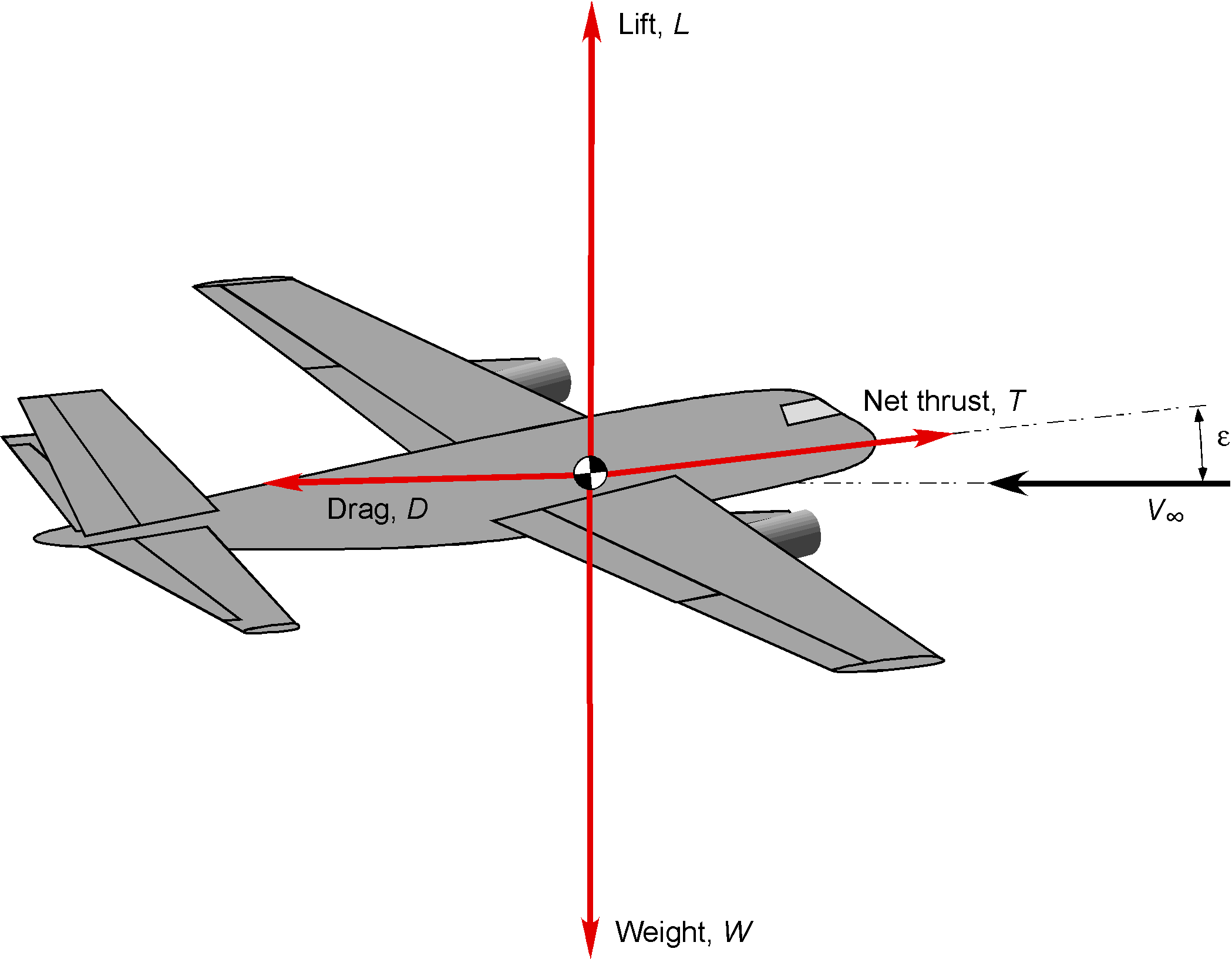
The performance characteristics of an airplane depend on its aerodynamic drag, as well as the characteristics of the engines that power it. A significant portion of the total aircraft drag originates from the wings, which are primarily influenced by the lifting area and aspect ratio of the wing, as well as the angle of attack and operational Mach number. However, the airframe drag and all other components, except the wings, are also significant contributors to the total drag of the airplane. For straight-and-level, unaccelerated flight conditions, with the assumption that  , then lift,
  , equals weight,
  , and thrust,
  , equals drag,
  , i.e.,
(1) 
Once the drag, (or an estimate for the drag), is determined, the thrust or power requirements for the flight can be determined at any given aircraft weight, , and operational altitude (i.e., the density altitude). Using the engine characteristics (thrust developed ant available,  , or power available,
  ), many performance characteristics of the airplane can be calculated, such as its fuel burn, maximum and minimum attainable flight speeds, rates of climb, ceiling, range, and endurance. Remember that the weight of an airplane decreases in flight as fuel is burned off, except in the case of an electric airplane.
Components of Drag
The thrust and power required for flight are at the heart of a flight performance analysis. The weight of the airplane can be estimated based on its takeoff weight and fuel burn, but determining the drag is a more complex matter. Theoretically, the drag of a body in a flow is defined as the aerodynamic force associated with the time rate of change of momentum in the direction of the freestream. This net loss of momentum is determined by comparing the flow far upstream and far downstream of the body. In lifting flows, particularly for wings, the downstream control surface, known as the Trefftz plane, is used to assess the momentum deficit and quantify the induced drag resulting from trailing vorticity.
The total drag on the airplane may be separated into several contributing components, each arising from distinct physical mechanisms:
- Skin friction drag: This drag source arises from the tangential shear stresses on the airframe surfaces. It is fundamentally viscous and cannot exist in an inviscid fluid. Skin friction drag becomes especially significant over large surface areas, such as wings and fuselages.
- Normal pressure drag: This drag results from the integrated effect of pressure acting normal to the airframe’s surface. The term arises from the fact that when pressure forces are resolved into components, normal to and parallel to the airframe surfaces, part of their effects act in the direction of the freestream and, therefore, contribute directly to drag. This component can be further divided into:
-
- Boundary layer normal pressure drag (Form drag): Also referred to as pressure drag, this type of drag arises from the separation of the boundary layer from the surfaces, which alters the pressure distributions. It is defined as the difference between the total drag associated with boundary layer losses and the skin friction component. The total boundary layer drag includes both the skin friction and boundary layer pressure drag components, and is associated with losses in total pressure (and total temperature for high-speed flows) across the boundary layer.
- Induced drag (Trailing vortex drag): Generated by the vortex system trailing behind any lifting surface, such as the wing and horizontal tail. This type of drag directly results from lift production and generally becomes prominent at lower airspeeds and higher angles of attack.
- Wave drag: Wave drag is a component of aerodynamic drag that arises from the formation of shock waves and the irreversible energy losses that occur in compressible flow, particularly near and above the speed of sound. This component is dominant in transonic, supersonic, and hypersonic regimes and is highly sensitive to the airframe’s geometry.
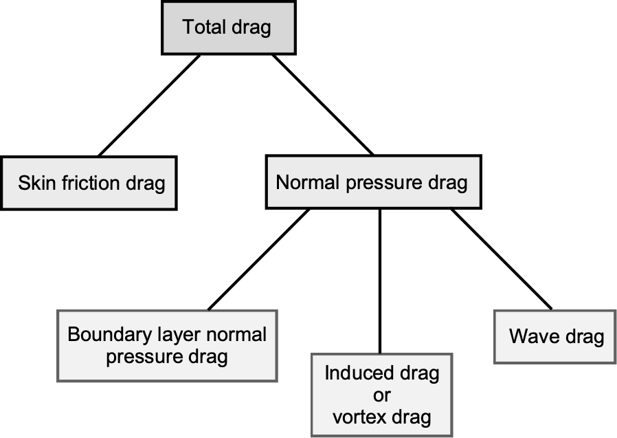
Breakdown of the drag components acting on a flight vehicle.
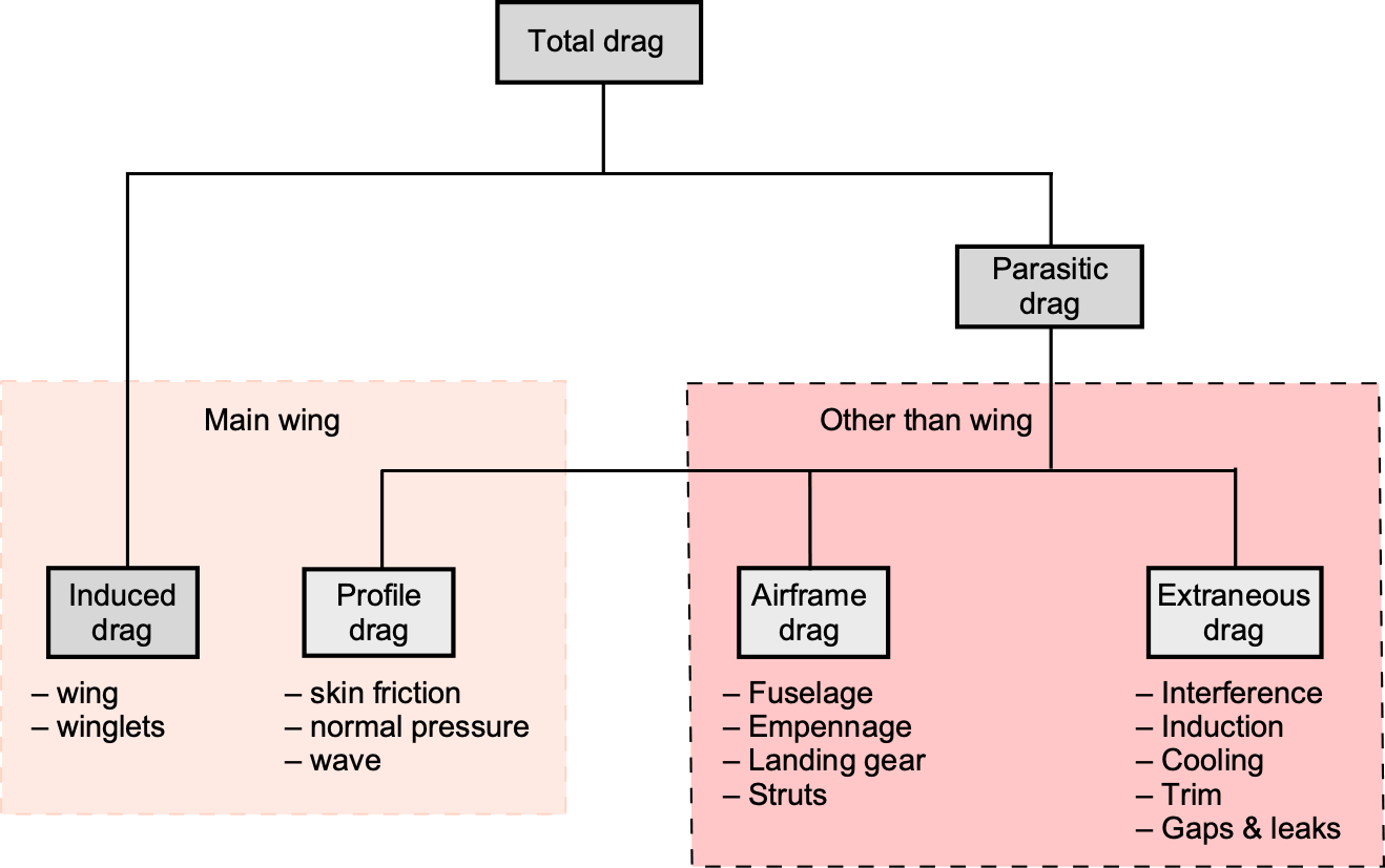
Parasitic drag is often used as a collective drag term in many contexts. Parastic drag includes both skin friction drag and form drag, in effect encompassing all drag components that are not associated with lift generation. In high-speed applications, parasitic drag becomes more significant because of higher skin friction, steeper pressure gradients, thicker boundary layers, and the onset of compressibility effects, i.e., wave drag. It must be carefully managed through streamlined airframe design and smooth surface finishes to minimize the cumulative drag buildup. Understanding these distinctions is essential for designing aerodynamically efficient flight vehicles.
Additional forms of drag, sometimes referred to as extraneous drag, may also become relevant depending on the flight regime and the configuration of the flight vehicle:
- Base drag: Arises from low-pressure separation zones at the rear of blunt-bodied vehicles, contributing significantly to total drag when wake regions are prominent.
- Interference drag occurs from flow interactions between different components of a flight vehicle, such as wing-body junctions or engine-pylon combinations. It is difficult to isolate, but must be minimized through careful integration.
- Trim drag: The extra drag caused by the deflection of the flight controls to achieve “trim,” i.e., force and moment equilibrium on the airplane.
- Spillage drag (Induction drag): Associated with external flow not adequately captured by the engine inlets. This is a critical concern in the inlets to supersonic engines.
- Cooling drag: Results from the ejection of coolant or bleed air used for thermal protection of the engines or airframe, which alters the net momentum balance of the vehicle.
- Gap & seal drag: Extra drag caused by imperfect seals between control surfaces and wings, undercarriage doors, cabin doors, etc.
Drag Model
The simplest drag model for an airplane is to represent its drag as an average non-lifting or parasitic value added to a lifting value that varies with the square of the lift coefficient, the breakdown being shown in the schematic below. The average drag value is independent of lift and, in the aggregate, accounts for the drag on all airframe surfaces, i.e., the sum of the skin friction and normal pressure drag over the wings, fuselage, empennage, etc., as well as extraneous drag contributions.
The other part of the total drag is called induced drag, as it is the drag generated by the airplane’s creation of lift. The physics behind this component is tied to the trailing vortex system behind the airplane, as previously discussed, and it is proportional to the square of the lift coefficient and hence to the square of the aircraft’s weight. The induced drag is the dominant source of drag at low airspeeds, but is inversely proportional to the square of airspeed, so it diminishes quickly at higher airspeeds. Parasitic drag is dominant at higher airspeeds and increases with the square of the airspeed.
Drag Equation
With these assumptions on the division of the drag components, the drag coefficient for the entire airplane can be expressed as
(2) 
where  is the induced drag coefficient and coefficient
  depends on the wing and overall aircraft design. Theoretically, the induced drag coefficient can be expressed as
(3) 
where  is the aspect ratio of the wing and
  (the value of is < 1) is called Oswald’s efficiency factor. Note that Oswald’s efficiency factor applies to the aircraft as a whole, not just to the wing, and includes non-ideal induced losses from other lifting components, such as the tail.
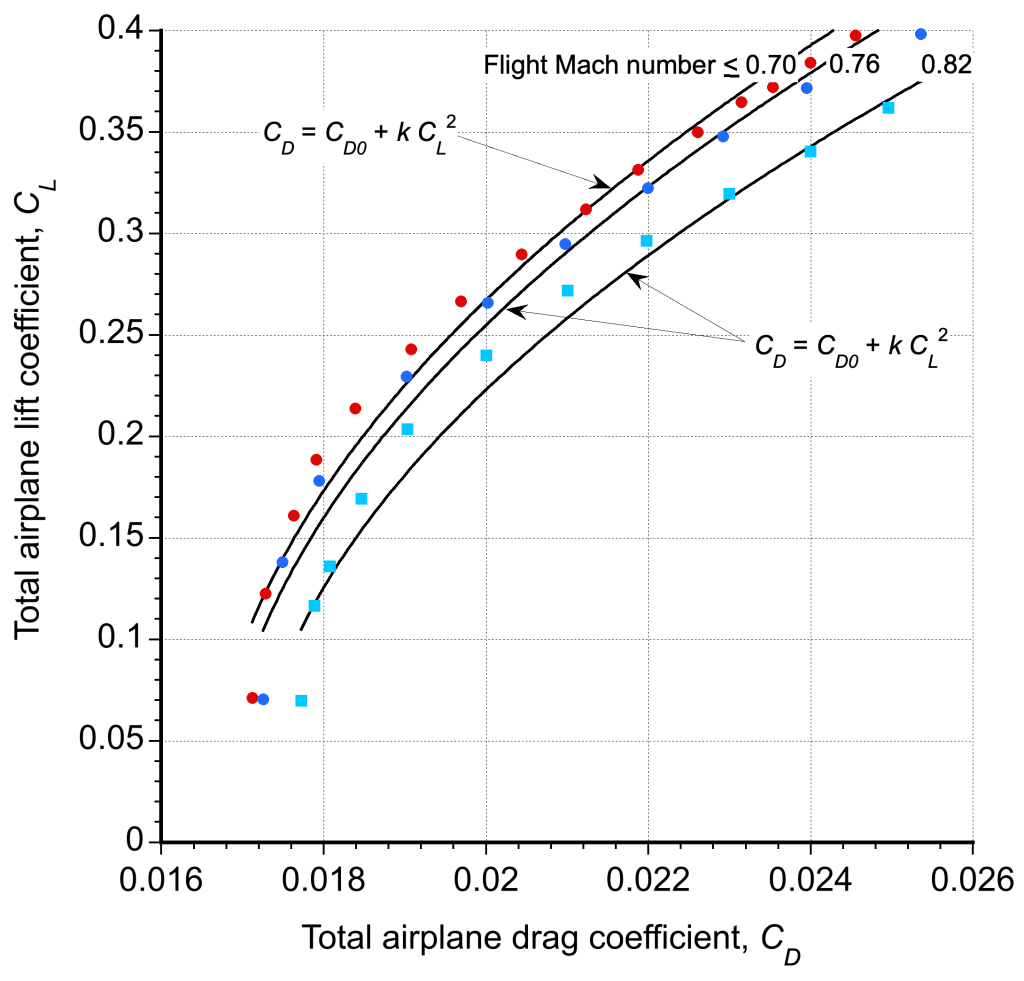
The validity of Eq. 2 has been established for various categories and classes of airplanes, as illustrated in the figure below for an airliner. While the fit is imperfect, it enables the derivation of analytical results, as well as those that are sufficient for at least preliminary estimates of airplane performance, until they can be verified through flight testing. In this case, the difference in the polar curves for the three Mach numbers is because of the buildup of wave drag. Instead of using an equation, a table-lookup process for the values of  at a given
  is an alternative approach, but this approach requires numerical methods.
Drag Synthesis
The total drag coefficient of an airplane can be expressed more precisely in terms of contributions from the wing, fuselage, and empennage, as well as component interference effects, the latter being the most difficult to estimate and can only be approximately accounted for. The process of determining an aircraft’s total drag by summing its components is known as a drag synthesis method.
Wing
Wing drag has a significant impact on the performance of all airplanes. Wing drag arises from two sources: the profile drag at the sectional level and the induced drag, i.e., the drag induced by lift production. The profile drag comprises skin friction and pressure drag, which can be obtained from two-dimensional airfoil data for the specific wing section. Such lift and drag data are readily available for many airfoil sections. As previously shown, a good approximation at the sectional level is
(4) 
where  is the non-lifting drag coefficient and
  is the growth in the drag coefficient with the sectional lift coefficient,
  . Assuming these preceding values can be suitably obtained based on measurements, which are generally available from airfoil data catalogs or other publications, and that each section of the wing operates at the same lift coefficient,
  , which is a reasonable assumption for an ideal, elliptically loaded wing, then the profile drag of the entire wing can be expressed as
(5) 
The induced drag of the wing is
(6) 
where  is the spanwise efficiency factor. For a perfect, elliptically-loaded wing,
  . For a well-designed airplane wing with appropriate wing taper and twist, it is reasonable to expect to be in the
  range. Therefore, the total drag of the wing can be expressed as
(7) 
Fuselage
Fuselage drag, while minimized through streamlining, can be significantly affected by various disturbances. These include surface roughness from rivets and panel joints, flow separation near blunt regions or poorly faired intersections, and protuberances such as Pitot tubes, antennas, and cooling inlets. Additional sources include landing gear doors, radomes, and empennage junctions, as well as factors like paint degradation or insect contamination. Although each may contribute only a small amount individually, their combined effect can noticeably increase overall drag.
The fuselage drag can be expressed as
(8) 
where  is determined based on the maximum cross-sectional area,
  , and slenderness ratio of the fuselage, and
  is the reference area, which is usually the wing planform area on which all aerodynamic coefficients are based, i.e.,
  . The coefficient
  accounts for the increased drag of the fuselage when it is operating at an angle of attack.
Empennage
The empennage consists of the horizontal and vertical tail surfaces, along with their respective controls, including the elevator and rudder. In trimmed flight, the vertical tail will produce little lift. The horizontal tail will produce some lift, but is small enough to be neglected in terms of induced drag contribution. Therefore, it is reasonable to represent the empennage drag as a profile contribution, i.e.,
(9) 
where  is the projected planform area of the tail surfaces in the aggregate, and
  depends on the specific tail design. Values of can be most reliably obtained from wind tunnel tests on scaled models at or near the Reynolds and Mach numbers of flight; historical data derived from flight tests are also useful.
Total Drag
The total drag on the aircraft is the sum of the preceding area-normalized drag components, i.e.,
(10) 
Note that all individual values of the drag coefficients have now been normalized to the same reference area, allowing them to be added directly without adjustment. Substituting the values gives
(11) 
Notice that it is now possible to group the preceding terms into non-lifting and lifting parts for the entire airplane, i.e.,
(12) 
or
(13) 
where the non-lifting part is
(14) 
and the lifting or induced part is
(15) 
This equation can also be written in the form
(16) 
where is Oswald’s efficiency factor.
The total drag values obtained from this form of synthesis are typically multiplied by an interference factor of 1.1 or 1.2 to account for airframe component flow interference effects, i.e.,
(17) 
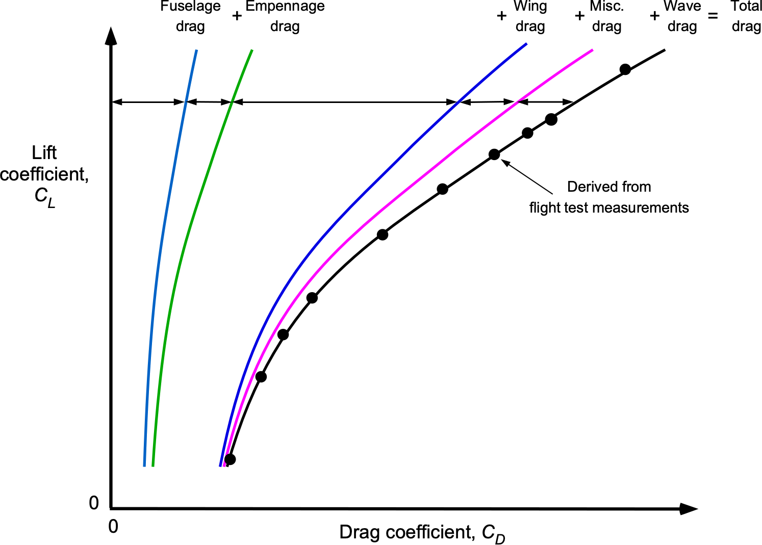
which accounts for the excess drag produced, for example, between the wing and the fuselage, and/or between the propulsion system and the airframe, etc. The basic idea is shown in the figure below, where the drag contributions from the individual components that comprise the airplane are logically quantifiable.
Wave Drag
Other sources of drag can affect the polar, such as wave drag (from the creation of shock waves) and stall effects. However, departures from Eq. 2 from stall will only affect the airplane’s performance at higher lift coefficients and higher gross weights that may be considered outside the standard operational flight envelope.
The growth of wave drag as the transonic flight regime is approached is nonlinear in terms of Mach number and angle of attack; therefore, developing a suitable mathematical model for drag is somewhat more complicated. One approach is to use the Lock model, as previously discussed. This model requires a value of the critical Mach number of the wing,  , which is the flight Mach number (defined as
  ) at which the onset of supersonic flow first appears.
The wave drag increment can be written as
(18) 
where  is a constant. Therefore, including the wave drag increment, the modified drag equation for the airplane can be written as
(19) 
While the Lock equation has been found to give reasonably good predictions of the extra wave, drag on an airplane, and the consequent effects on the polar, quantitative predictions for a specific airplane depend on the value of . For example,  is often used for an airliner designed to cruise in transonic flight where
  . For airplanes with thin, supersonic airfoils with higher critical Mach numbers,
  is more appropriate.
Thrust & Power Required for Flight
The total (dimensional) drag on the airplane, , is then
(20) 
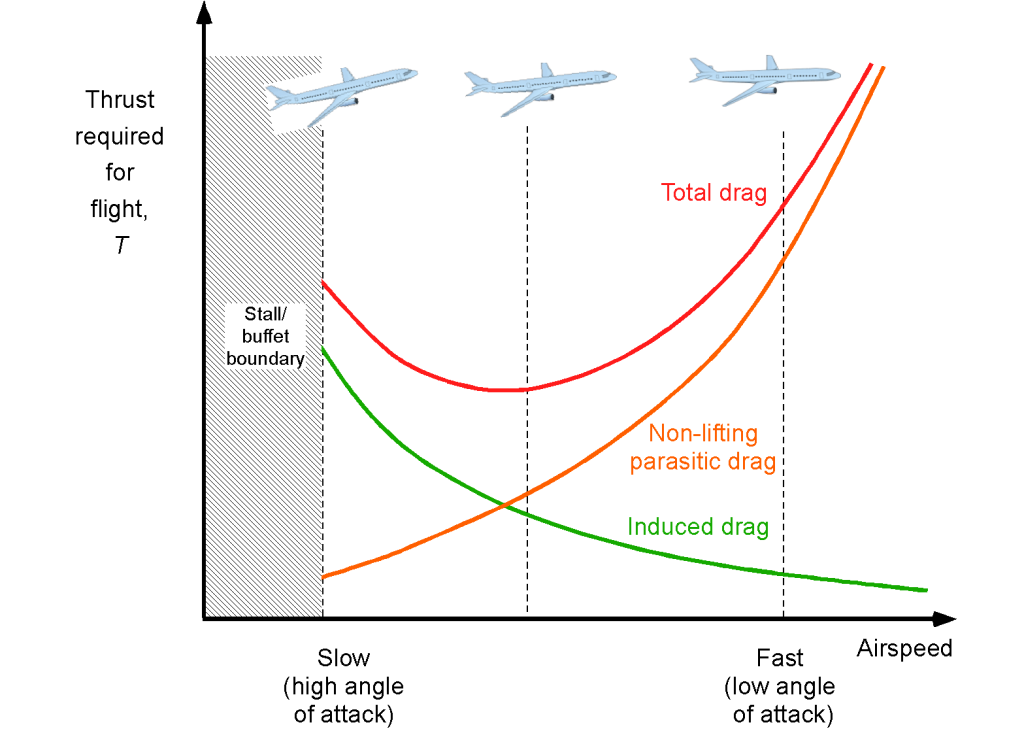
A representative variation of drag is shown in the figure below. The aircraft’s true airspeed through the air is denoted by  . Notice that the drag must be equal to the thrust required,
  , needed from the propulsive system for steady flight when lift equals the in-flight weight, i.e., in balance flight or trim, then
(21) 
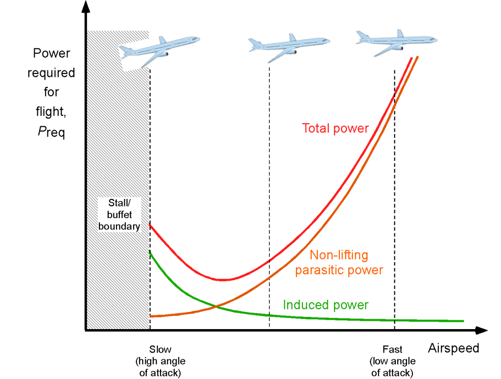
The corresponding power required for flight is then
(22) 
as shown in the figure below, which again has a characteristic U-shaped curve. Notice that the power required for flight at a given in-flight weight increases rapidly when the airplane flies faster.
Calculation of In-Flight Weight
In the following sections and chapters, there will be frequent references to the aircraft’s in-flight weight. The weight of an aircraft at a given time during its flight is not fixed and depends on the weight of fuel being burned off, which in turn depends on airspeed, altitude, thrust, throttle setting, and engine characteristics, such as specific fuel consumption (SFC). For many aircraft, the weight of fuel to be carried for the flight is a significant fraction of the takeoff weight. Therefore, the weight of the fuel burned off must be known to determine the in-flight weight accurately. However, for many performance calculations, the in-flight weight at any point in the flight can be assumed or estimated based on the takeoff weight, along with a reasonable average estimate of the fuel burn, e.g., in units of weight per hour.
The aircraft’s gross weight on the ramp before taxiing to the runway will be the sum of its empty weight,  , plus the useful load,
  . The aircraft’s empty weight comprises its structure, engines, internal fixtures, oil, hydraulic fluids, and all other components necessary for it to be ready to fly without carrying any payload or fuel. The useful load is the sum of the payload,
  , and the fuel weight,
  . Payload is the weight the aircraft carries onboard that pays the bills, such as passengers, baggage, and cargo. However, fuel is not considered payload; it is a useful load.
The takeoff weight must always be less than or equal to the aircraft’s maximum allowable (certified) gross weight,  . Therefore, the gross takeoff weight of the aircraft,
  , will be
(23) 
Another way of expressing this latter sum is in terms of weight fraction, i.e., a component weight as a fraction of the gross weight. Therefore,
(24) 
where the  values are called weight fractions.
If the average fuel burn rate for the aircraft can be established, i.e., an estimate for  , then the in-flight weight, , after a given time
  since the takeoff can be obtained by integration, i.e.,
(25) 
The minus sign indicates that weight is reduced as fuel is burned off.
However, for initial estimates of aircraft performance, including flight range and endurance, it is common to use an in-flight weight equal to the gross weight less half the usable fuel weight at the takeoff condition. A more advanced calculation will estimate or measure the fuel burn during different phases of the flight, including taxi, takeoff, and climb, to better estimate the in-flight weight. Nevertheless, whatever aircraft weight is used for the performance calculations, its value and how it is calculated should always be qualified based on the best available information.
Jet-Propelled Airplane
Consider the performance analysis of a jet-propelled airplane. For the steady level flight condition where  , then
(26) 
which assumes that there is no extra compressibility drag (i.e., wave drag) at high cruise Mach numbers. The equation to be solved is
(27) 
Because in steady flight  then
then
(28) 
where  is the air density in which the aircraft is flying,
  is the reference wing area, and is the total wing lift coefficient (the assumption here is that the wings generate all of the lift). Notice that
  where the value of
  comes from the ISA model, i.e.,
(29) 
Rearranging this equation, the lift coefficient that needs to be produced on the wing for a given flight speed can be solved for, i.e.,
(30) 
Therefore, after some algebra, the drag becomes
(31) 
which, for steady level flight, is the thrust required for flight, .
To express this latter result more compactly, define constants  and
and  as
as
(32) 
Then the drag curve simplifies to the canonical equation
(33) 
This expression shows the nature of the drag curve. The first term in this latter equation (the profile or zero-lift drag) becomes dominant at higher airspeeds, and the second term (the induced drag) becomes larger at lower airspeeds; the resulting drag curve is U-shaped, as shown previously. Notice also the effects of weight on the induced drag, which is proportional to  .
.
Therefore, the equation to be solved is
(34) 
This problem can be solved graphically, which is easy to visualize, as discussed below, or numerically.
Thrust Available
Now, consider the engine thrust. The maximum thrust from a jet engine is available only at sea level. It decreases with an increase in altitude, i.e., the density decreases and the thrust available declines for a given throttle setting. Throttle settings are generally specified as takeoff, maximum continuous, cruise, and idle, but military aircraft may also have an afterburner thrust selection.
The thrust available (the output of the jet engine) depends on many things, specifically the airspeed, the density of the air in which the airplane is flying (i.e., the density altitude), and the throttle setting ( ). Therefore, the available thrust from the engine can be written the general form
(35) 
Consequently, for a given density altitude, airplane weight, and engine throttle setting, both the thrust available (from the engine) and the thrust required (equal to the aircraft drag) become a function of airspeed and/or Mach number.
Thrust Required
To achieve level flight, the horizontal equilibrium equation must be satisfied (Eq. 27 or Eq. 34) for a given weight and altitude. To solve the equation, both the thrust available from the engine and the thrust required (i.e., the drag of the aircraft) must be plotted versus the airspeed (or Mach number), and then the precise conditions where the curves coincide must be determined, as shown in the figure below. At that point, Eq. 34 will be satisfied, so the airspeed and the thrust required for a given weight and altitude can be determined.
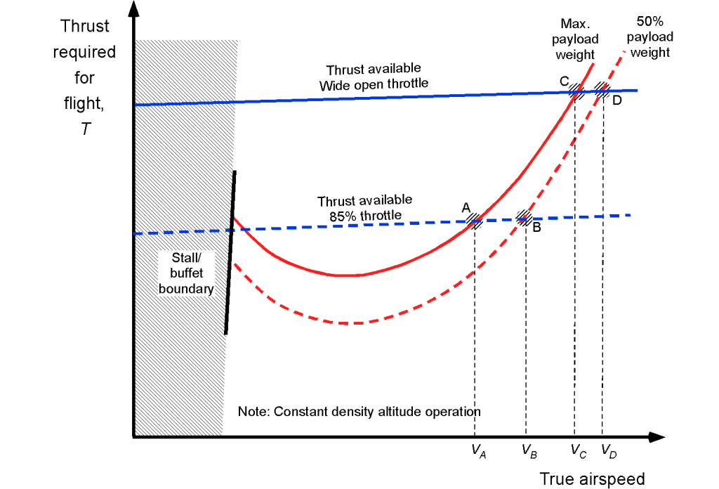
Notice that the thrust available and the required curve can intersect at two points. The intersection at the highest airspeed corresponds to the maximum flight airspeed for that aircraft at the particular density altitude, aircraft weight, and throttle setting. The possibility of an intersection at lower airspeeds will be the minimum airspeed the aircraft can maintain level flight at that altitude, and is called the thrust-limited minimum airspeed. In some cases, this airspeed may exceed the stall airspeed. Generally, an airplane’s safe minimum flyable airspeed at a given altitude will be greater than the thrust-limited minimum or stall airspeed. However, in the clean configuration (i.e., no flaps, gear up), the stall airspeed is usually the higher of the two airspeeds.
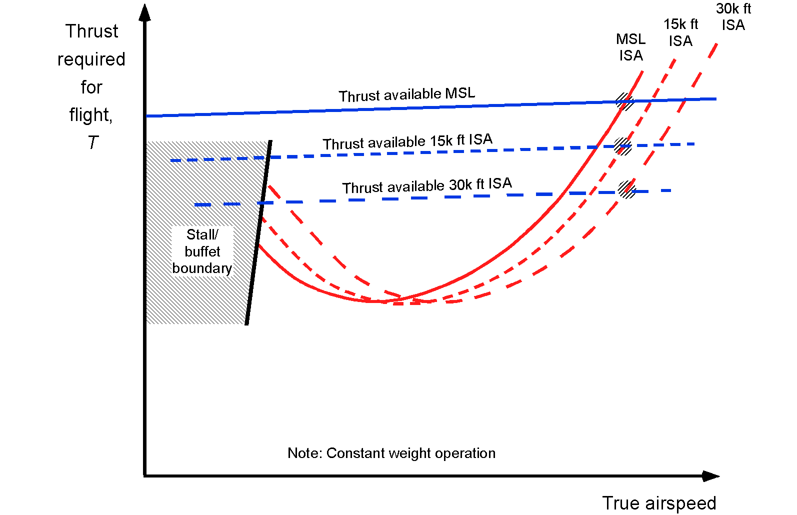
The thrust available and the thrust required curves versus airspeed can be plotted for each altitude and weight of interest. Of course, the exact quantitative relationships between power and airspeed depend on the detailed aerodynamics of the actual airplane, as well as the characteristics of the engines, which, as previously mentioned, may only be available in numerical form, e.g., tables. As altitude increases and air density decreases, the maximum thrust available at a given throttle setting decreases, as shown in the figure below. These intersection points represent the maximum and minimum airspeeds at which the aircraft can fly at each altitude, given a specific weight and throttle setting, thereby determining the airspeed flight boundary. Notice that at higher altitudes, the achievable lowest airspeed becomes thrust-limited, while at lower altitudes, the attainable speed is generally determined by the onset of stall.
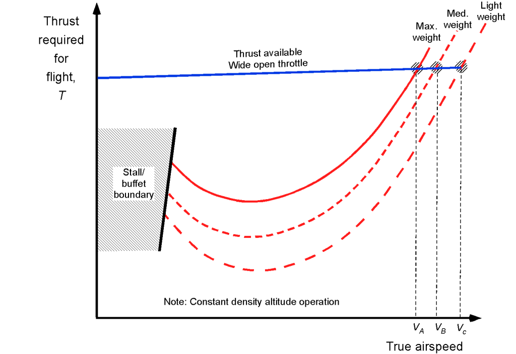
There will eventually be an altitude at which the available thrust approaches the minimum drag, where the available thrust curve intersects the required thrust curve at a single point. This condition corresponds, to a certain extent, to the aircraft’s maximum achievable altitude or ceiling. Notice from the figure below that changing the aircraft’s weight significantly affects the thrust curves because the lift coefficient increases at lower airspeeds, and the induced drag increases. As shown in the figure below, increasing flight weight tends to shift the thrust required curve up and slightly to the right.
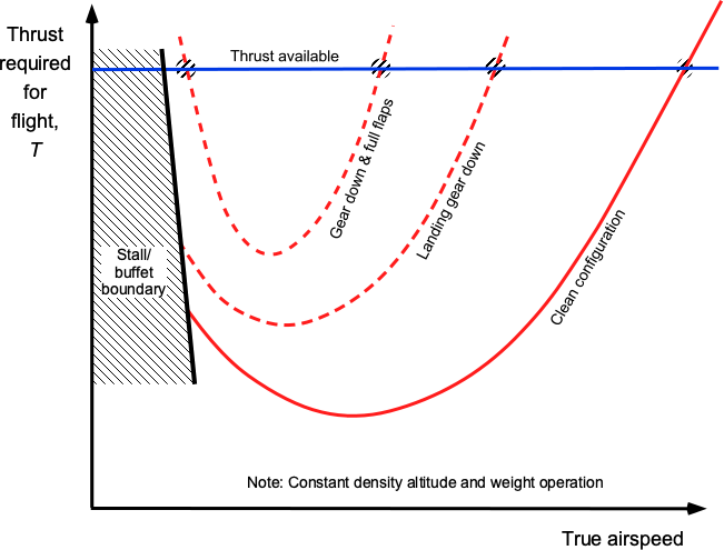
The effect of configuration also affects the thrust required for flight, as shown in the figure below. The clean configuration refers to the normal flight condition with flaps and slats (if any) extended and the landing gear retracted. Lowering the landing gear significantly increases drag, and the deployment of the flaps further exacerbates this drag, resulting in the “dirty configuration.” Notice in the figure that the flight envelope (or corridor) is increasingly constrained between the thrust available from the engines and the stall speed of the aircraft. In the dirty configuration with landing gear down and full flaps, the thrust-limiting airspeed is reached before the onset of stall. In this case, such narrow allowable airspeed corridors necessitate precise flight control during the landing phase.
While these graphical results are fairly easy to interpret, the problem can also be solved analytically under some conditions. Take, for example, a jet-powered airplane, where it can be assumed that the propulsive thrust is not substantially dependent on airspeed for a given altitude, i.e., where it is reasonable to assume that  constant for a given altitude. The airspeed of the airplane can be found from
(36) 
After some algebra and rearrangement of terms, the airspeed for thrust and drag equilibrium can be obtained by solving the quartic equation
(37) 
where
(38) 
Notice that these coefficients contain both the thrust-to-weight ratio and the wing loading. While there are multiple roots to Eq. 37, not all of them are physical, and only two of these roots will have significance.
It can be shown that the jet airplane can maintain level flight at a given altitude if
(39) 
which is naturally and intrinsically tied to the aircraft’s aerodynamic characteristics. The limiting condition of this latter result occurs at the ceiling of the aircraft when the minimum and maximum attainable airspeeds coincide, which is
(40) 
However, this value can only be determined explicitly if the engine thrust is known. As previously discussed, it is a function of density altitude and throttle setting.
In most cases, the preceding problem must be solved numerically or graphically. The procedures described would apply to any variations in airplane drag or engine thrust. The propulsion characteristics of engines are often presented in graphs or tables for engineering analysis, allowing the calculation of thrust at various airspeeds and altitudes. Similar procedures are used to develop a more detailed model of the drag on the aircraft, including the effects of wave drag. For high-performance aircraft, such results are typically determined using a combination of calculations, wind tunnel tests, and flight tests. They are generally made available as tables as functions of the angle of attack and Mach number.
Propeller-Driven Airplane
Consider now a propeller-driven airplane. Remember that the output of an engine driving a propeller (e.g., a turboshaft or a piston engine) is quantified in terms of power. However, it must also be recognized that this power is converted into thrust according to the aerodynamic characteristics and performance of the propeller. There may be some jet thrust from a turboshaft, but it is usually small enough to be ignored.
The power required for flight can be written as
(41) 
where  can be considered as the net propulsive efficiency of the propulsive system (engine and propeller combined); notice that this value may not be a constant and will generally vary with airspeed depending on the type of propeller system.
Splitting the foregoing equation (Eq. 41) into its two parts, leads to
(42) 
The first term in the preceding equation is the non-lifting part, and the second is the induced part. Notice that the power associated with the non-lifting part increases with the cube of the airspeed. As previously shown, the second (induced) part depends on the lift coefficient, which reduces with increasing airspeed.
Using Eq. 30 gives
(43) 
so the power required equation now becomes
(44) 
which, after some simplification, leads to
(45) 
This latter equation is in the form
(46) 
where in this case
(47) 
Notice that the non-lifting part increases with the cube of the airspeed, but the lifting part decreases inversely with airspeed.
Power Available
The power available for flight is a characteristic of the powerplant, i.e., all the power that could be delivered from the engine to drive the propeller and propel the airplane forward. If the shaft power available from the engine is  (this is called its brake power), then the power available for flight (or sometimes denoted as
  ) will be
(48) 
This result shows that the propeller efficiency reduces the available power for flight, i.e., not all of the power at the engine shaft can be delivered as useful work to the air by the propeller.
The actual power required for flight depends on the drag of the airplane, so
(49) 
For steady-level flight at a constant airspeed and altitude, the pilot needs to set the throttle so that the power required for flight is equal to the power available, i.e.,
(50) 
so that the brake power needed from the engine will be
(51) 
Shaft power versus air power.
In performance analyses, the brake (shaft) power matters because the power delivered at the shaft ultimately affects the engine’s fuel consumption. The higher the propeller efficiency, the lower the brake power required, resulting in lower fuel consumption. The power that can be delivered to the air in terms of useful work, known as airpower, depends on the propeller’s efficiency.
Naturally, the power available from the powerplant may be greater or less than the power required for flight. For example, any excess power available over and above that otherwise needed for level flight at a given weight, airspeed, and altitude will allow the airplane to accelerate to a higher airspeed and/or climb to a higher altitude. For this reason, the airplane’s initial takeoff and climb performance is strongly affected by the power available from the powerplant.
Power Required
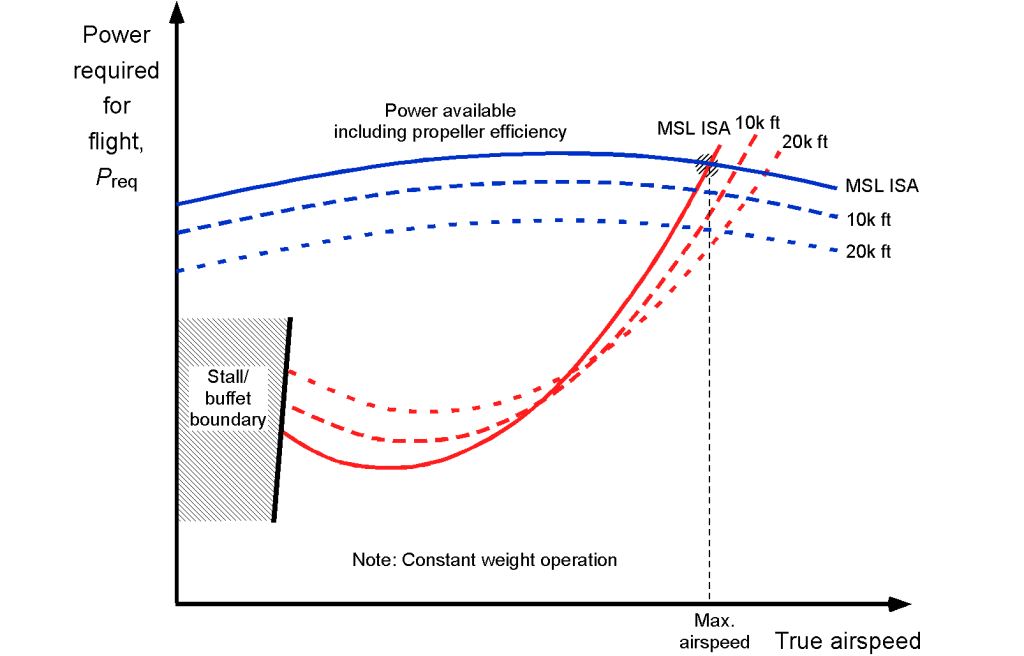
The figure below shows representative power-required curves for a propeller-driven airplane. Higher power is required at lower airspeeds, a minimum range of power is needed for some intermediate airspeeds, and then a rapid increase in power (with the cube of the airspeed) is required as higher airspeeds are reached. Aircraft that use propellers will have charts in terms of airspeed and flight Mach number, with the propeller’s helical tip Mach number being critical.
The lowest possible flight airspeed is generally limited by the onset of wing stall and/or buffeting from the onset of flow separation, often causing the aircraft to shake, regardless of the available power. At higher weights and/or density altitudes, the rapid increase in power required will eventually limit the maximum level flight airspeed of the airplane for a given weight and operational altitude, assuming no other limits or barriers to flight appear.
The power available typically increases with airspeed and levels off over the airspeed range where the airplane generally flies. The figure below illustrates that the power available decreases with altitude. Again, analogous to the manner for the jet aircraft, the level flight solution is the intersection of the available power curves and the power required curves. The highest airspeed solution is the maximum level flight airspeed, which is achieved at a given altitude, aircraft weight, and throttle setting. However, the minimum speed solution is only valid if that speed is greater than the aircraft’s stall speed. Again, the aircraft’s ceiling can be determined at the airspeed at which the minimum power for flight coincides with the available power.
Assuming that and the propulsive efficiency remain constant for all weights and airspeeds, the airspeeds can be solved in closed form. This is a special case, but a reasonable assumption for a constant-speed propeller with the engine operating at wide-open throttle. After some algebra, the equation to be solved is
(52) 
where
(53) 
from which the maximum and minimum speeds can, in principle, be solved for. However, this problem is more difficult because the relevant equation is nonlinear.
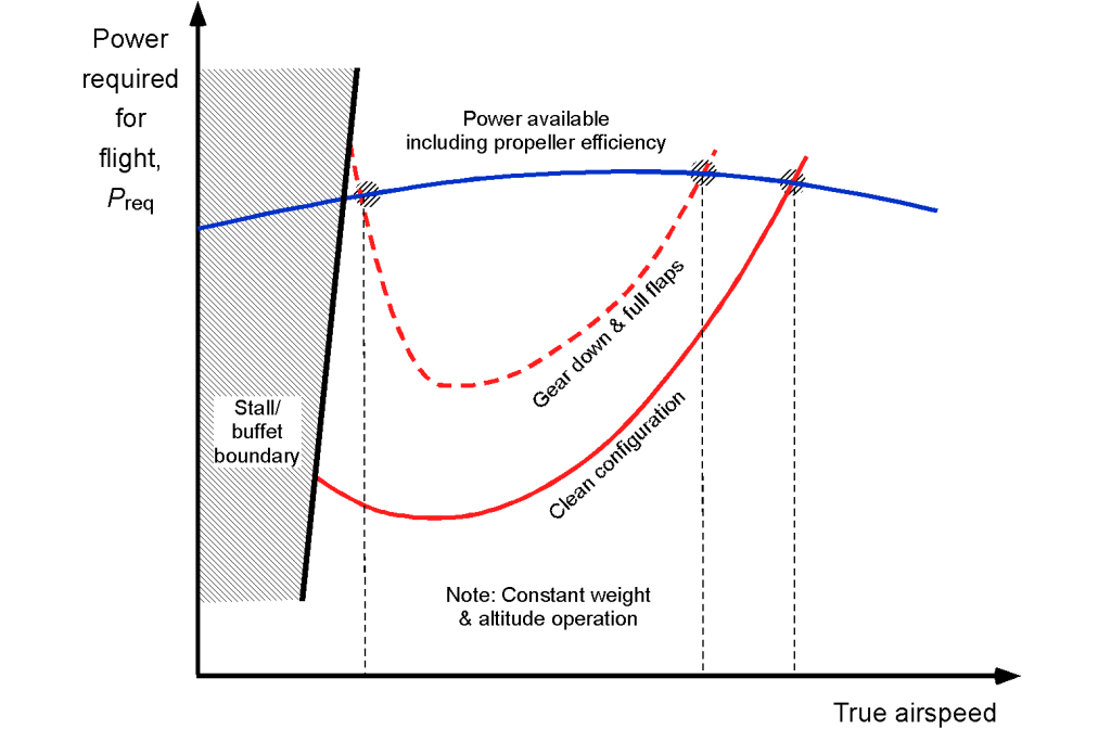
The effect of configuration, i.e., clean or dirty with the flaps up or down, landing gear up or down, etc., also affects the power required, as shown in the figure below. As with jet-powered aircraft, notice that the flight envelope becomes increasingly constrained between the available power and the stall speed. In the dirty configuration with landing gear down and full flaps, such as for landing, it is possible that a power-limiting airspeed can be reached before the onset of the stall. In this regard, the pilot must ensure that the airplane has sufficient excess airspeed in case of a go-around and that sufficient excess power is available to climb away from the runway.
Drag Polar & Equivalent Weight Method
While the drag polar can be estimated from a combination of component drag synthesis and aerodynamic theory, the often-asked question is how to extract the drag polar from flight tests, which is central to completing validated performance analysis. The answer is obtained using the equivalent weight method (EWM), a technique that normalizes flight data collected under varying in-flight weight and atmospheric conditions. The EWM can be used to estimate the coefficients in the drag polar, i.e., the non-lifting drag coefficient,  , and Oswald’s efficiency factor, .
During flight testing, the airplane’s weight changes (unless it is electrically powered) because of fuel burn or payload variations, and atmospheric conditions, such as pressure, temperature, and air density, change with altitude and the time of day. These changes affect airspeed measurements and the thrust or power required for flight, making direct performance comparisons difficult when they are taken over many flights at different in-flight weights over several days, weeks, or months. The EWM addresses this issue by transforming measured quantities into equivalent values referenced to a standard weight and sea-level density. This normalization process enables the accurate extraction of aerodynamic performance parameters and from measurements taken under various flight conditions. Although originally developed for conventional aircraft, the method can be adapted to electric and unoccupied platforms such as drones with appropriate care, making it a versatile tool in flight performance analysis and validation of performance models.
Equivalent Weight Velocity
The development of the EWM starts with the assumption that in straight-and-level unaccelerated flight, the lift on the airplane is equal to its weight, so that
(54) 
where  is the true airspeed of the aircraft through the air and is the reference (planform) wing area. Notice that the true airspeed must be determined from the indicated airspeed with corrections for altitude,[1] mechanical errors, and static position errors. Measurements will often be performed at a given (set) pressure altitude to ensure consistency between tests conducted over long periods of time.
The equivalent weight velocity,  , is defined in terms of the reference weight for the aircraft,
  , and MSL ISA density,
  , as
, as
(55) 
where the reference weight, , is usually the maximum gross weight of the airplane and is the MSL ISA value. Therefore, it can be seen that
(56) 
(57) 
and this is the definition of the equivalent weight velocity. Notice that the is normalized by both density and weight.
Equivalent Weight Power
The power required for flight can be written as
(58) 
where is the drag on the airplane, which is equal to the thrust, . Also, in straight-and-level flight, then
(59) 
Substituting this relationship into the power equation gives
(60) 
Defining the equivalent weight power required as
(61) 
(62) 
Again, notice that  is normalized by both density and weight. Reliable thrust or power estimations require onboard instrumentation to measure the engine’s key operating parameters, which can be related to the thrust or power from the engine’s calibration tests.
Determining the Drag Polar
Calculating the equivalent weight velocity, , and the equivalent weight power, , is the first step in the analysis. The final step is determining the zero-lift drag coefficient and the span efficiency factor . In the proceeding, the drag polar can be assumed to have the standard parabolic form, i.e.,
(63) 
Using the flight test data, the following procedure is used:
- Convert all measured airspeeds, , and power values,
 , to their equivalent weight forms, i.e., and , using Eqs. 57 and 62 given above.
 - The equivalent weight power can also be written as
(64)

where the drag on the airplane is assumed to equal the thrust from the propulsion system, i.e.,
= . Recall that determining the power required for flight,  , will require access to engine calibration data and measurements made of key engine operating parameters. This step is critical because it provides the basis for computing the in-flight power requirement and the aerodynamic drag.
 - Substitute the assumed drag polar for to get
(65)

Because
can be related to using(66)

then
(67)

Substituting and multiplying through by
gives(68)

This equation is in the form
(69)

where
(70)

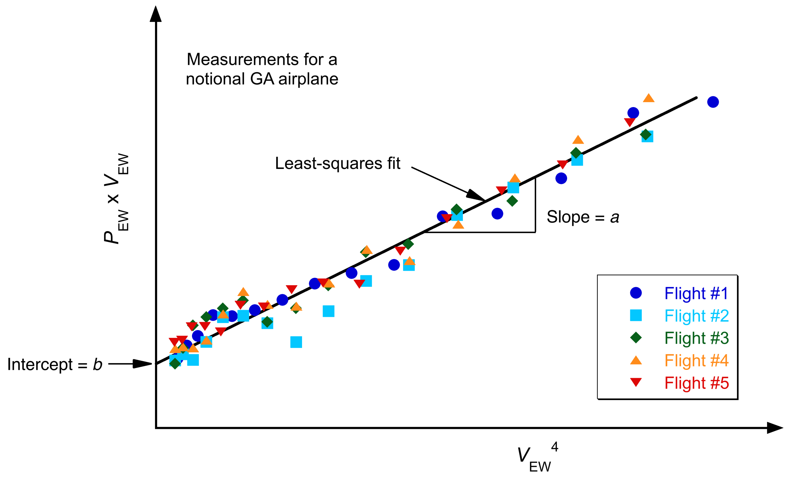
- Finally, plotting
 versus
  for all measured points yields the required parameters, as shown in the figure below. The slope and intercept are obtained from a least-squares fit to the measured flight test data, which typically comprises data from several flights over a range of airspeeds, weights, and atmospheric conditions. The parameters of the drag polar are then given by
(71)

Application of the EWM to Different Aircraft Types
Several practical cases of interest involve the use of the EWM. Conventional aircraft burning fuel will experience a gradual weight decrease over time, which can be measured by subtracting the net fuel burned from the takeoff weight, based on measured fuel flow rates. The EWM can be applied for various payloads and fuel loads to normalize performance data and derive consistent drag polar parameters. In each case, estimating the power required, , requires knowledge of the engine power output as a function of various measurable parameters and engine calibration maps. Notice that for an electrically powered airplane, its weight will not change unless a payload is ejected.
- Propeller-driven aircraft with piston engines: The shaft power can be estimated using engine instrumentation that provides rotational speed (RPM), manifold pressure, throttle setting, altitude (pressure and temperature), and air density. Engine calibration charts specific to the installed engine are then used to determine the corresponding shaft power. This shaft power can be converted to thrust using the propeller’s efficiency, , which depends on the advance ratio,
 , i.e.,
(72)

where
is the true airspeed,  is the propeller rotational speed in revolutions per second, and is the propeller diameter. Access to propeller performance curves, commonly referred to as “ curves”, is required to estimate as a function of and blade pitch setting. With these inputs, the propulsive thrust can be inferred from
(73)

also allowing the in-flight power requirements to be determined.
- Propeller-driven aircraft with turboshaft engines: Power estimations in this case must rely on turbine-specific engine parameters such as torque, propeller rpm, fuel flow, interstage turbine temperature (ITT), and pressure altitude. Many turboprop aircraft are equipped with torque sensors, which directly measure the torque delivered to the propeller shaft. The shaft power is computed from
(74)

where
 is the measured shaft torque. The thrust is then calculated using the propeller curves, as for the piston engine.
 - Jet-powered airplane: Estimating thrust and power for jet-powered aircraft requires knowledge of engine performance maps as a function of Mach number, altitude, and throttle setting. Accurate in-flight thrust estimation depends on access to calibrated engine performance data, combined with measured parameters such as fuel flow, engine pressure ratio (EPR), fan speed (N1 or N2), and total air temperature. In practice, thrust is determined from manufacturer-supplied performance models or test-derived correlations that relate thrust output to these operating conditions.
- Electric aircraft or drones: These typically operate at near-constant weight over short missions, allowing the method to account for variations in atmospheric conditions (e.g., density changes with altitude or time of day). Test points can also be gathered using various payload configurations. In this case, electric motor power and voltage/current measurements are used directly, assuming well-characterized efficiency maps for the battery and motor.
Avian Flight
The natural evolution of birds over hundreds of millions of years has led to sophisticated adaptations that enable them to thrive in their aerial environment. These adaptations are shaped by natural selection, which favors natural fliers with specific biological characteristics that enhance their flight performance. Therefore, the question is whether the performance of avian fliers behaves in the same manner or even in a similar manner to that of airplanes.
Even a casual observation reveals that birds exhibit a wide range of wing shapes, each tailored to their specific flight requirements. For example, birds adapted for long-distance soaring, such as hawks, eagles, pelicans, and albatrosses, have long, high-aspect-ratio wings that allow them to glide almost effortlessly. In contrast, birds adapted for hovering, such as hummingbirds, have short, low-aspect-ratio wings with low inertia, enabling them to hover in place and maneuver with great agility. These avian wing forms are not random but have been shaped by evolution and constrained by the physical laws that govern aerodynamics.
The complex nature of the reciprocating flapping wings of birds poses additional challenges in understanding their flight performance characteristics. Unlike aircraft, birds must generate propulsion by flapping their wings, which requires specific adaptations in the muscular and skeletal system to produce aerodynamic forces. The upshot continuously changes flight parameters during each wingbeat, such as wing area, wingspan, aspect ratio, and angle of attack. The flapping motion also creates unsteady flows around their wings. It makes estimating flight forces and power requirements more complicated compared to steady-level flight of an airplane.
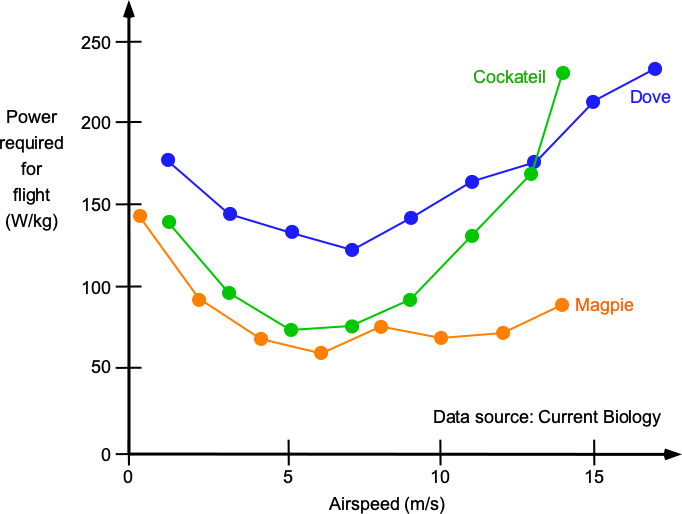
However, the same fundamental principles of aerodynamics that apply to airplanes should also apply to the wings of birds. For example, the shape of a bird’s wing generates lift by creating differences in air pressure between the upper and lower surfaces of the wing, just like an airplane wing generates lift. The effects of the wing tip vortices must cause induced drag, as with an airplane’s wing. To this end, biologists have measured the flapping power birds require for flight in wind tunnels, necessitating measurements of metabolic rates or other methods. Birds can be trained to fly in the wind tunnel, although the measurement approaches have relatively high experimental uncertainty. Nevertheless, the figure below shows that the characteristic U-shaped power curve for an airplane is obtained, with the induced drag dominating the power for flight at low flight speeds.
The unique characteristics of flapping wings also provide birds with notable advantages in flight compared to airplanes. The ability of birds to adapt their wing shapes enables them to quickly change flight situations. Birds can also adaptively twist their wings to adjust the angle of attack and lift distribution, allowing them to perform agile maneuvers, the hummingbird being an exquisite example.
In recent years, aeronautical engineers have taken inspiration from these natural fliers to explore new ideas of mechanical flight, such as for micro air vehicles that can mimic wing-beat movements. Indeed, the evolution of flight in birds is an excellent example of how biology can inspire other engineering solutions. By understanding the physical laws governing flight and studying the forms and structures of natural flyers, engineers may gain new insight into designing more efficient and maneuverable aircraft. However, it should also be remembered that avian fliers have developed under evolutionary and biological constraints that engineers are not so encumbered by.
Summary & Closure
The analysis used to quantify level flight performance depends on the type of airplane, specifically whether it is jet-propelled or propeller-driven. The primary difference is that the output of a jet engine is measured in terms of its thrust production, whereas the output of an engine driving a propeller is measured in terms of its power output. A significant portion of the total aircraft drag originates from the wing, which is influenced by its angle of attack and the flight Mach number. However, the airframe drag and all other components, except the wing, are also significant contributors to the total drag of the airplane. Once the drag (or an estimate for drag) is determined, the thrust or power requirements for flight can be determined at any given aircraft weight and operational density altitude. Using the engine characteristics (thrust available, power available, and specific fuel consumption), many performance characteristics of an airplane can now be calculated.
5-Question Self-Assessment Quickquiz
For Further Thought or Discussion
- Consider adding a term to the drag polar to account for the onset of wave drag. How will this change the thrust required curve?
- If an airplane’s aerodynamic characteristics are available only in table format (e.g., tables of lift and drag), consider how these results can be incorporated into the analysis to determine the aircraft’s performance characteristics.
- Under what conditions might the minimum level flight airspeed of an airplane be higher than its stall speed?
- Why does the thrust available from a turboprop system decrease quickly at higher airspeeds?
- In steady-level flight, how does the aircraft’s drag vary with airspeed? Explain the factors that contribute to this relationship.
- Discuss the concept of induced drag during steady-level flight. How does it vary with changes in angle of attack and airspeed?
- How does the wing loading affect an aircraft’s steady level-flight performance?
- What are the limitations and considerations associated with maintaining a steady level flight near the aircraft’s maximum ceiling?
- Discuss the impact of wing aspect ratio on an aircraft’s steady level-flight characteristics. How does it affect lift, drag, and fuel efficiency?
- Describe the impact of engine performance, including power output and fuel efficiency, on steady-level-flight operations. Explain the relationship between specific fuel consumption and range.
- Discuss the challenges and considerations associated with maintaining steady-level flight in supersonic aircraft.
Other Useful Online Resources
To learn more about the level flight performance characteristics, follow up with some of these more practical online resources:
- Recall that an altimeter is calibrated based on MSL ISA density. ↵
