24 Boundary Layer Flows
Introduction
To further study other types of flow, including those about airfoils and wings, the effects of viscosity must be considered. In fact, lift generation on a wing is fundamentally a viscous phenomenon. However, in most flows over surfaces, including those internal and external to the surfaces, viscosity effects are confined to a thin flow region known as the boundary layer. Viscous effects will always be significant when fluids flow across surfaces. The boundary layer is a fundamental concept in aerodynamics and fluid dynamics, as it substantially influences a body’s overall aerodynamic characteristics, including its lift and drag.
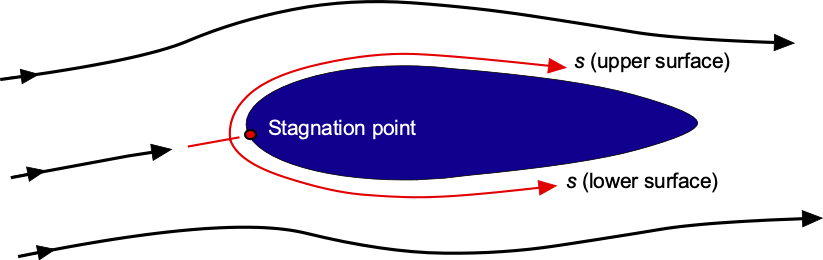
For example, the figure below illustrates the boundary layer concept as it develops over the upper and lower surfaces of an airfoil. In this boundary layer region, viscosity effects are significant, and what occurs here is critically important, as it affects the aerodynamic characteristics of the airfoil section or any other body. However, it should be noted that boundary layers are much thinner in reality than the relative dimensions of the zones shown in this figure. Notice that the boundary layer “grows” as it develops downstream, i.e., its thickness and other properties change with downstream distance.
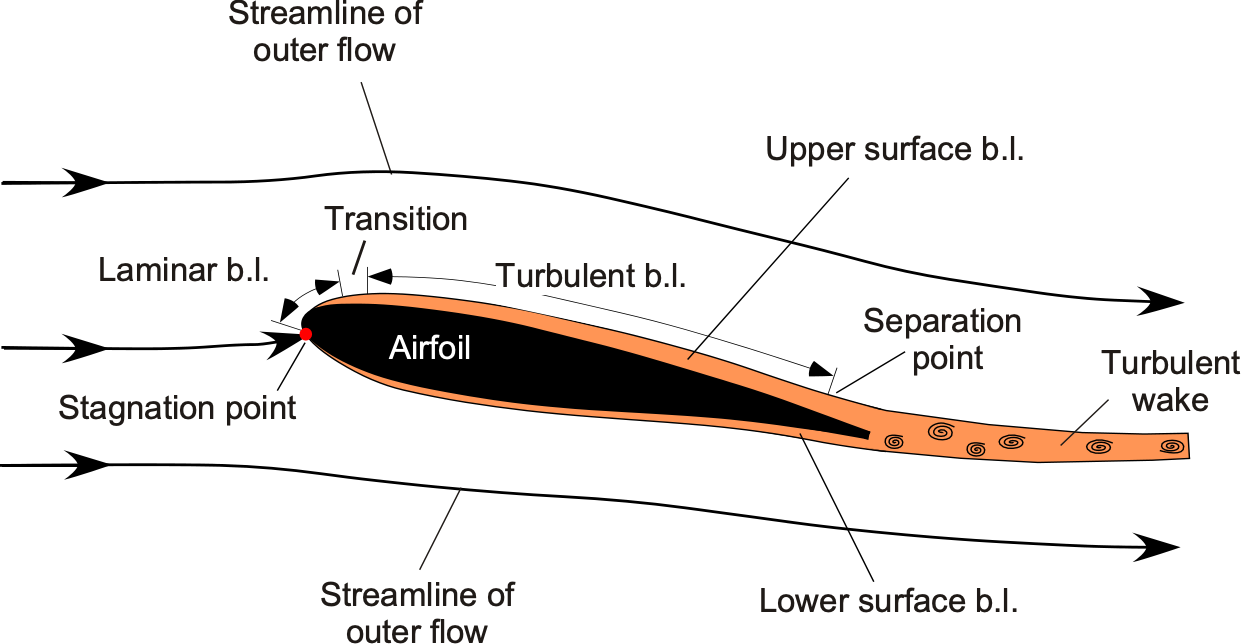
One effect produced by the development of the boundary layer over a body is the creation of shear stresses on its surface, the cumulative manifestation of which is skin friction drag. Skin friction is a significant source of overall drag on an aircraft, particularly in high-speed flight, where it accounts for approximately half of the total drag. Another effect is that boundary layers can thicken and detach or separate from surfaces under certain conditions, a phenomenon called flow separation. The onset of boundary layer flow separation from a surface generally has a deleterious effect on its aerodynamics, with a loss of lift and the creation of drag. In many cases, the aerodynamic characteristics of lifting surfaces and other bodies can only be explained with a knowledge of the underlying boundary layer behavior.
Learning Objectives
- Understand the basic concept of a boundary layer and appreciate its physical significance as it can affect aerodynamic flows over airfoils, wings, and other body shapes.
- Distinguish between the primary characteristics of laminar and turbulent boundary layers.
- Know how to calculate the shear stress on a surface under the influence of a boundary layer for particular types of velocity profiles, and be able to estimate skin friction drag.
- Understand why and under what conditions boundary layers may detach or separate from surfaces and what subsequent effects may be produced.
- Know some essential characteristics of thermal boundary layers.
History
Historically, Ludwig Prandtl introduced the concept of the boundary layer. His work on the subject originated from experiments made with his students in Germany at the beginning of the 20th century. Prandtl showed that for fluids with relatively small viscosity that flow over surfaces or bodies, the effects of the internal stresses in the fluid are appreciable only in a region near the fluid boundaries, which he called a boundary layer. Understanding boundary layers and their effects on flow development was a significant step forward in expanding knowledge of fluid dynamics. Before this, in the 17th century, Isaac Newton discovered that fluids could be deformed. Because of the relative motion between their layers, shear stresses are created in the fluid, resulting in what is now known as Newton’s law of viscosity. Newton also noted that there is no relative motion between the fluid and a solid surface (the “wall”), which is known as the no-slip condition.
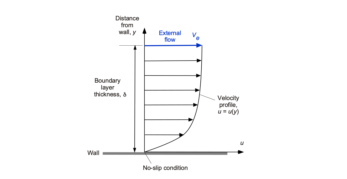
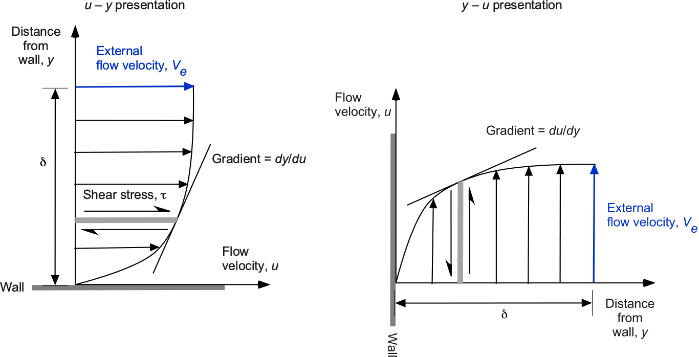
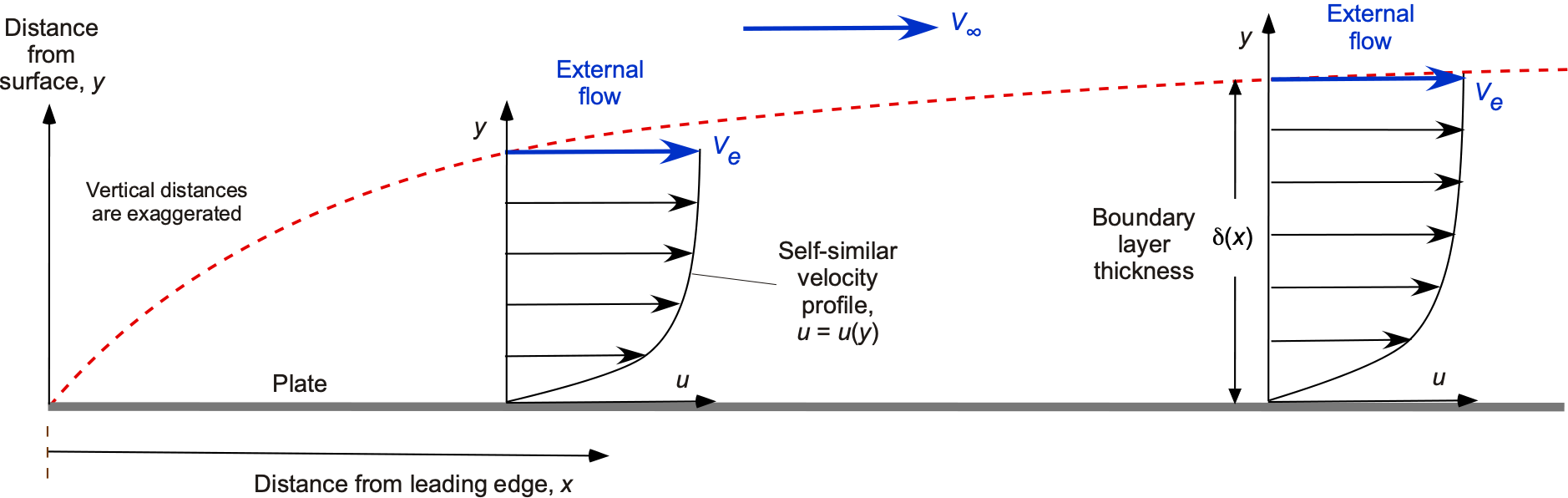
As shown in the figure below, the flow velocity in a boundary layer rises quickly from zero at the surface (no-slip condition) and then smoothly and asymptotically approaches the external flow velocity,  , as the distance increases from the surface. However, it should be appreciated that a boundary layer is very thin; the vertical extent or thickness of the boundary layer is given the symbol
  . The boundary layer is said to have a shape or profile, i.e., the velocity in the boundary layer parallel to the surface,
  , varies as a function of the distance from the surface
  , i.e., in functional form, then
  . The form of the boundary layer profile depends on several factors, including the nature of the surface and the effects produced by the external flow, such as pressure gradients.
Different types of boundary layers exhibit distinct velocity profiles; however, as will be discussed, they are typically characterized as either laminar or turbulent boundary layer profiles, each having similar yet distinct flow characteristics. In general, what occurs within the boundary layer is crucial in aerodynamics and fluid dynamics. One is that it affects the shear produced on a body’s surface over which the boundary layer develops and, therefore, the magnitude of the net skin friction drag created on the body. The properties of the boundary layer also determine whether the flow remains attached to the body’s surface or separates from it.
Laminar & Turbulent Boundary Layers
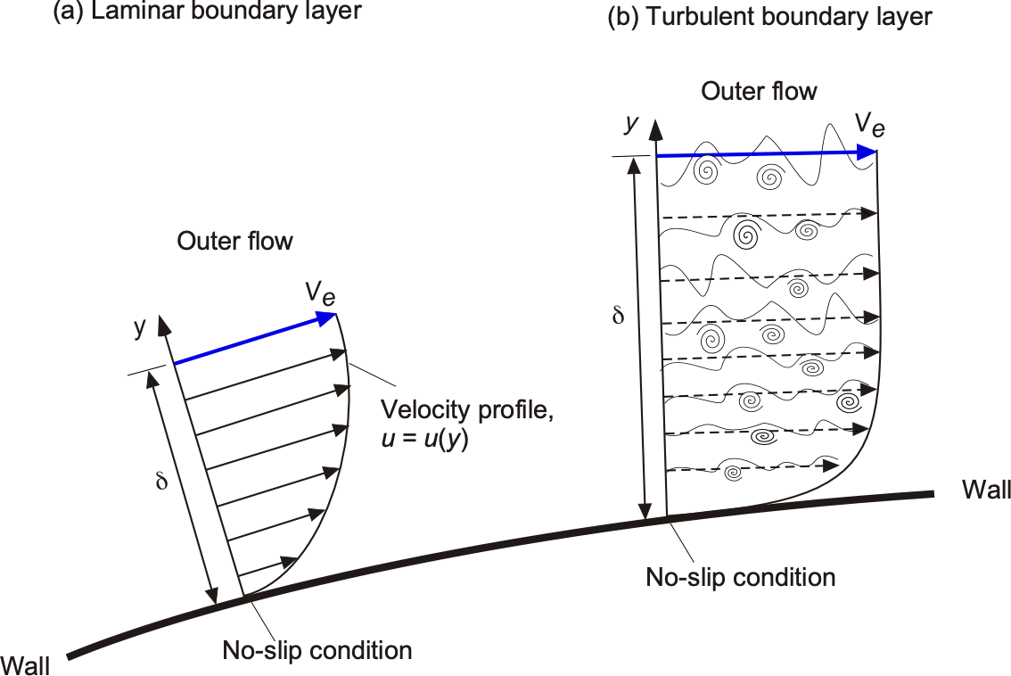
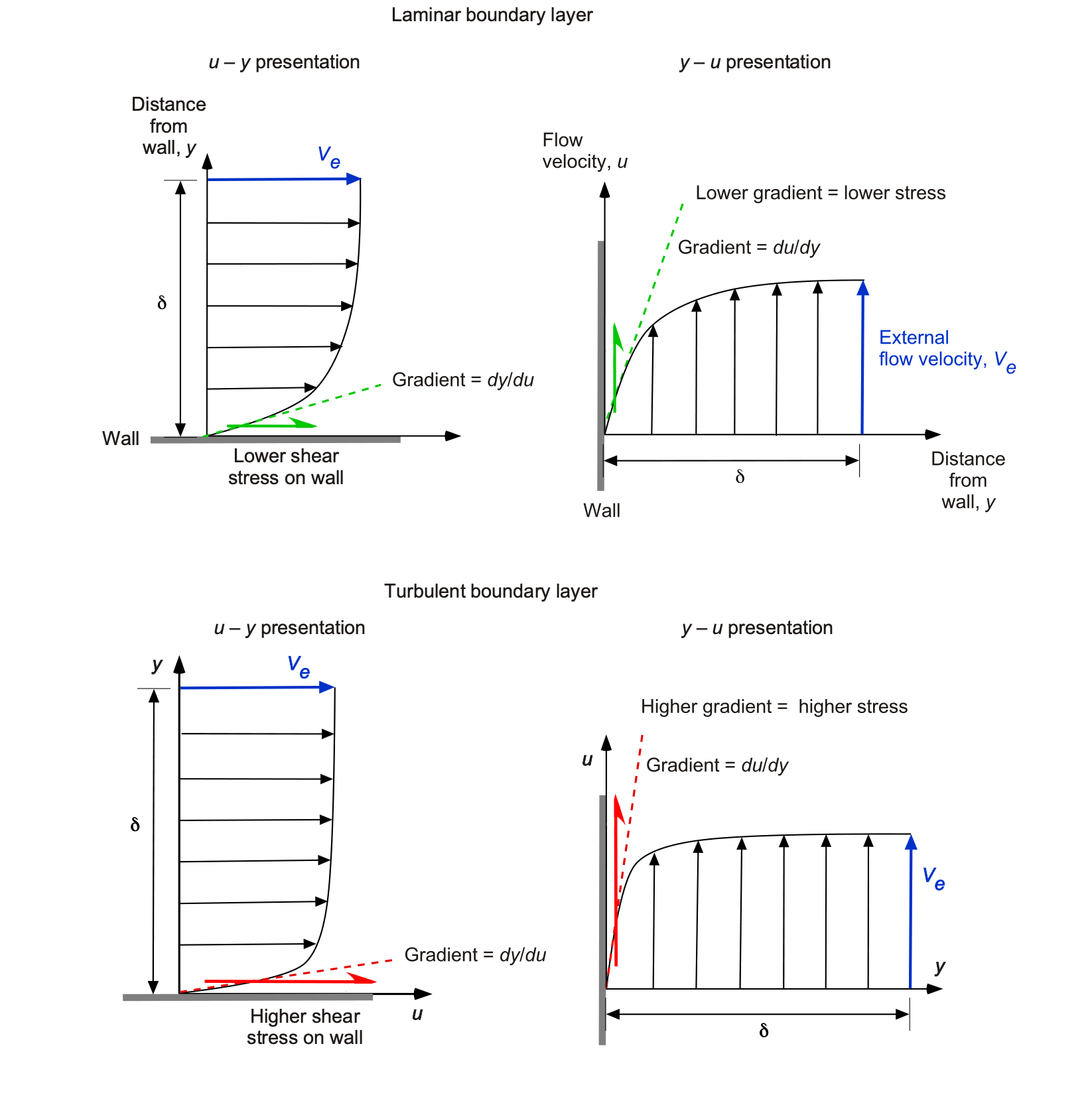
As detailed in the figure below, in a laminar boundary layer, the fluid flows orderly, with smooth layers that are free of mixing between successive layers; such layers are called laminae, from which the “laminar” name is derived. The fluid layers in a turbulent boundary layer become mixed, so the flow velocities away from the immediate region at the wall tend to be more uniform. Due to the rotational motion of the fluid and the resulting shear stresses, vortical eddies and turbulence are also formed, leading to significant mixing in the flow. Turbulent boundary layers are inevitably thicker than laminar boundary layers because the effects of flow mixing extend further away from the wall.
Another useful quantitative comparison of the profile shapes of a typical laminar and turbulent boundary layer is shown in the following figure. This presentation is obtained by normalizing the velocity profile by the boundary layer thickness and the outer or edge velocity of the external flow, , i.e., by plotting  as a function of
  . Note that in the case of a turbulent boundary layer, would represent the mean or time-averaged flow velocity, not the instantaneous velocity.
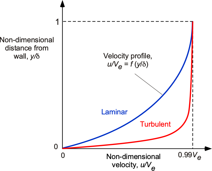
Boundary layer profiles are nearly always plotted in this non-dimensional form because it then allows for ready comparison of their velocity profiles for given values of and , i.e., they are in the general functional form
(1) 
where  is the form of the velocity profile, so
  at the edge of the boundary layer when
  . Notice that the velocity gradients, i.e.,
  , in a laminar boundary layer are relatively shallow throughout compared to a turbulent boundary layer.
Because the velocity in the boundary layer smoothly and asymptotically approaches the external flow velocity, the value of must be defined rather carefully to avoid ambiguity. By convention, is defined as the value of for which 99% of the external flow velocity is recovered, i.e., when  .
.
Shear Stresses & Skin Friction
It has already been discussed that viscous stresses in fluids are produced whenever there is relative motion between adjacent fluid elements, and these stresses produce a resistance that tends to retard the motion of the fluid. The viscous shear stress,  , is related to the absolute viscosity,
  , by using Newton’s law of viscosity formula, i.e.,
(2) 
where  is the rate at which the flow velocity increases (in the direction) and is equivalent to a strain rate, as explained in the figure below. A characteristic of fluids is that they must be continuously deformed (strained) to produce shear, unlike solid materials, where an applied strain always maintains a residual stress. Therefore, a fluid must be continuously deformed to create stresses; when the strain rate is removed, the fluid will relax to an unstrained state. The strain rate is
  , so the shallower the value of this gradient, the lower the shear stresses.
Due to mixing in a turbulent boundary layer, its velocity profile becomes more uniform away from the wall. However, this case has steeper velocity gradients as the wall is approached. Because of the flow mixing in a turbulent boundary layer, it develops a greater thickness, , than a laminar boundary layer that forms under the same flow conditions. Equation 2 is a general expression that applies to any point in the flow. However, it is restricted to fluids that behave such that they follow a linear stress/strain relationship, i.e., a so-called Newtonian fluid where the slope of the stress/strain-rate relationship is linear, and so the value of is constant.
Aerospace engineers are particularly interested in the shear stress produced on the surface or “wall” over which the boundary layer flows, i.e., what happens as  , because this value determines the skin friction drag produced by the boundary layer on the surface. The stress in the fluid at the wall, which is in the upstream direction, has a reaction shear on the wall in the downstream direction. At the wall, the shear stress is
(3) 
(4) 
As implied by the shape of the boundary layer velocity profiles, as shown in the figure below, the magnitude of the wall shear stress,  , produced in the boundary layer (and hence on the wall) will be greater if a turbulent boundary layer flows over it compared with a laminar one.
This latter result is significant because the development of the boundary layer is the primary source of shear stress drag, also known as skin friction drag, on a flight vehicle. Therefore, it would be desirable to generate low drag by having a laminar boundary layer over as much of the vehicle as possible. However, in reality, it is found that laminar boundary layers do not exist for very long in terms of the downstream distance over which they develop, and so they become turbulent.
Nevertheless, calculating the shear stress caused by the boundary layer is a prerequisite to calculating the drag on any body shape exposed to a flow. As might be expected, drag prediction is challenging for entire aircraft or other flight vehicles because they have complex shapes and three-dimensional flows. In this case, the boundary layers also take on more complicated three-dimensional forms.
Development of a Boundary Layer
It should be appreciated that a boundary layer is not a static phenomenon. It is said to “grow” as it develops with downstream distance over a surface. Thus, the thickness and other properties of a boundary layer will change continuously as it develops downstream over any given surface. Furthermore, the development of a boundary layer may also be affected by other factors, such as pressure gradients and surface roughness.
A classic example studied by all engineering students is a boundary layer that develops on the top surface of a smooth flat plate set at zero angle of attack to the oncoming flow, i.e., a uniform velocity flow. Because the surface is flat without curvature, no pressure gradients will be produced over the surface. As shown in the figure below, the thickness of the boundary layer is zero at the leading edge of the plate. Its thickness then grows progressively and asymptotically, meaning that its growth rate is initially significant, and then it slows down as the boundary layer develops further downstream. Note that the vertical scale in the figure below has been exaggerated for clarity, and boundary layers are actually very thin. As previously mentioned, the thickness of the boundary layer, , can be defined at the height above the surface where the flow velocity on the boundary layer approaches the external or edge flow velocity, .
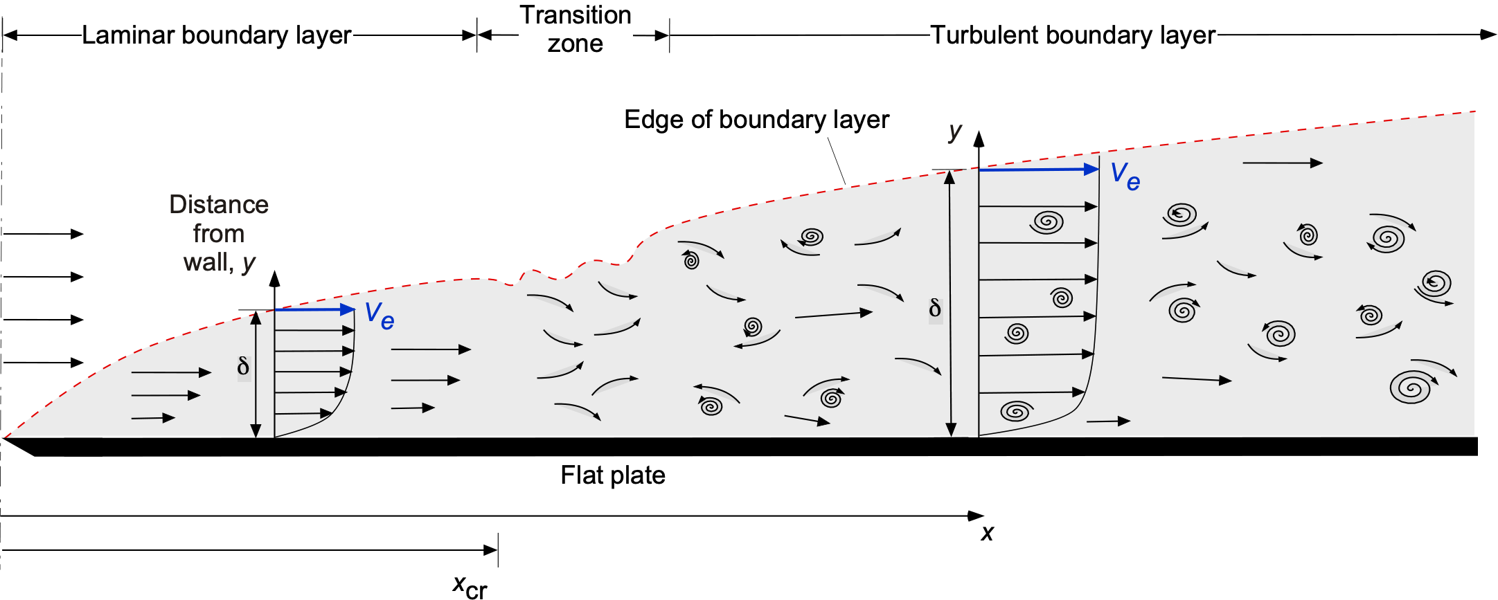
The boundary layer typically begins in a laminar form, at least over smooth surfaces, where the fluid moves in smooth, layered laminae or lamina-like motion. As the laminar boundary layer increases in thickness and develops downstream, the fluid layers naturally tend to mix. The location of transition, which happens over a finite distance, depends primarily on the Reynolds number. Finally, the boundary layer transforms itself into a well-mixed turbulent boundary layer. Even when the boundary layer becomes turbulent, a thin layer of laminar flow remains next to the wall, known as the laminar sublayer.
Notice that while turbulent boundary layers have a greater thickness than laminar boundary layers, it should be remembered that the velocity profiles of laminar and turbulent boundary layers are also different. While boundary layers are of two primary types, laminar and turbulent, the third type can be considered transitional. A transitional boundary layer is not fully developed because it is neither laminar nor turbulent. However, it usually exists in this form only for a relatively short zone or downstream distance.
Check Your Understanding #1 – Determining the shear stress in a boundary layer
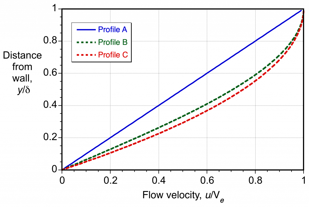
![\[ \mbox{\small Profile A:} \quad \frac{u}{V_e} = \frac{y}{\delta} \]](https://eaglepubs.erau.edu/app/uploads/quicklatex/quicklatex.com-a2b7d790193e0a97ceaeb4ca5403f6be_l3.svg "Rendered by QuickLaTeX.com")
![\[ \mbox{\small Profile B:} \quad \frac{u}{V_e} = \sin \left( \frac{\pi}{2} \frac{y}{\delta} \right) \]](https://eaglepubs.erau.edu/app/uploads/quicklatex/quicklatex.com-e7d73a4f5690d07ea80bba996547ed49_l3.svg "Rendered by QuickLaTeX.com")
![\[ \mbox{\small Profile C:} \quad \frac{u}{V_e} = 2 \left( \frac{y}{\delta}\right) - \left(\frac{y}{\delta} \right)^2 \]](https://eaglepubs.erau.edu/app/uploads/quicklatex/quicklatex.com-133ae4379f21c88b49da9067c611ffa3_l3.svg "Rendered by QuickLaTeX.com")
where is the flow velocity at the edge of the boundary layer, is the distance from the surface, and is the boundary layer thickness. Determine the relative shear stress on the wall for given values of and .
Show solution/hide solution.
Notice that all three profiles are of the laminar type, characterized by relatively low velocity gradients throughout. Notice that this is also a one-dimensional flow problem with velocities that only vary in the direction, so the shear stress on the wall in each case is given by evaluating
![\[ \tau_w = \mu \left( \frac{du}{dy} \right)_{y/\delta\rightarrow 0} = \mu \left(\frac{V_e}{\delta} \right) \left( \frac{d (u/V_e)}{d (y/\delta)} \right) \]](https://eaglepubs.erau.edu/app/uploads/quicklatex/quicklatex.com-015ccc23732d807d6ef424e7d4d0fa3b_l3.svg "Rendered by QuickLaTeX.com")
Therefore, for Profile A:
![\[ \frac{d (u/V_e)}{d (y/\delta)} = 1 \]](https://eaglepubs.erau.edu/app/uploads/quicklatex/quicklatex.com-9cb440b4e00a3d72bdea3277524e5cd6_l3.svg "Rendered by QuickLaTeX.com")
And for Profile B:
![\[ \frac{d (u/V_e)}{d (y/\delta)} = \frac{\pi}{2} \cos \left( \frac{\pi}{2} \frac{y}{\delta} \right) = \frac{\pi}{2}~\mbox{ as $y/\delta\rightarrow 0$} \]](https://eaglepubs.erau.edu/app/uploads/quicklatex/quicklatex.com-72b651710ab2d28351f9e4dbac038f40_l3.svg "Rendered by QuickLaTeX.com")
And, finally, for Profile C:
![\[ \frac{d (u/V_e)}{d (y/\delta)} = 2 \left(1 - (y/\delta) \right) = 2~\mbox{ as $y/\delta\rightarrow 0$} \]](https://eaglepubs.erau.edu/app/uploads/quicklatex/quicklatex.com-956420c4f55c6836fc842fc16b224785_l3.svg "Rendered by QuickLaTeX.com")
Based on the exact value of and also the same external flow velocity , the grouping
![\[ \mu \left(\frac{V_e}{\delta} \right) =~\mbox{constant} \]](https://eaglepubs.erau.edu/app/uploads/quicklatex/quicklatex.com-b66d550cb3e0d1b7d27faa2804a22098_l3.svg "Rendered by QuickLaTeX.com")
is the same, so it becomes clear that Profile A has the lowest relative shear stress and Profile C has the highest. Reinspection of the results plotted in the figure above readily confirms this.
Distance-Based Reynolds Number
The developing nature of the boundary layer can be characterized in terms of a local Reynolds number, which is measured in terms of the distance  from the point where the flow initially develops on the surface, i.e.,
(5) 
For example, as previously discussed,  is measured from the leading edge of a flat plate to some downstream distance. The boundary layer will often develop downstream from a stagnation point on a body, as shown in the figure below. Generally, the downstream distance will differ for the upper and lower surfaces and will depend on the geometric shape of the surface.
Transition
Experiments on smooth external flows over surfaces have shown that the boundary layer generally becomes naturally turbulent at Reynolds numbers based on  above about
  . The reason is that natural flow disturbances develop even over perfectly smooth surfaces, even those with mildly favorable pressure gradients, and cause a transition to a turbulent boundary layer. In this case, the value of the “critical” Reynolds number for transition to be initiated is denoted by
  , and the corresponding value of is denoted by
  , i.e.,
(6) 
and so
(7) 
Many experiments with airfoils and wings have examined the transition process from laminar to turbulent boundary layer flows. In all cases, the transition region has been found to correlate strongly with the Reynolds number based on downstream distance. For a smooth NACA 0012 airfoil, the critical Reynolds number for laminar-turbulent transition has been consistently shown to be approximately 10 ^5 at moderate to high angles of attack. However, the critical Reynolds number will depend somewhat on the shape of the airfoil. On most wings and airfoils, the transition region occurs just downstream of the minimum pressure at the leading edge.[1] Laminar boundary layers are sensitive to adverse pressure gradients because of their low velocities near the wall.
Because turbulent mixing during transition occurs progressively, the transition from a fully laminar boundary layer to a fully turbulent one happens over a certain distance. It is not a fixed point, per se. Although this distance is usually relatively small, perhaps 1% to 2% of the chord, it is still finite. In some cases, the transition will occur at the point where a short laminar separation bubble forms on the surface, which is typical for airfoil sections at chord Reynolds numbers over 10 .
.
Other Properties of Boundary Layers
Besides the velocity profile or  in the boundary layer, there are three other parameters that engineers use to quantify the characteristics of boundary layers, namely:
1. The displacement thickness,  .
.
2. The momentum thickness,  or
or  .
.
3. The shape factor,  .
.
Displacement Thickness
The displacement thickness of a boundary layer is given the symbol  and is defined by
(8) 
the idea of which is illustrated in the figure below.
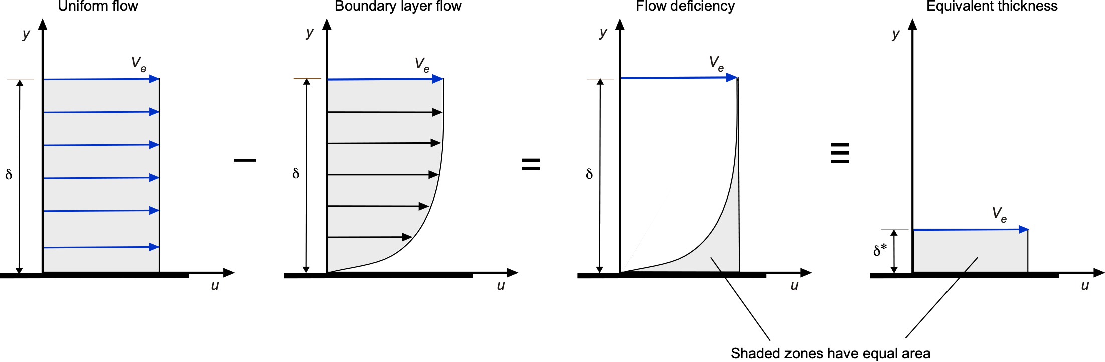
Notice that for conservation of mass in the boundary layer per unit depth, then
(9) 
where it will be remembered that is the value of when . On rearrangement, this gives
(10) 
and, finally,
(11) 
Therefore, the displacement thickness of a boundary layer can be interpreted as equivalent to the height or thickness corresponding to the reduction in mass flow associated with the boundary layer profile, which is, in effect, a mass flow deficit relative to the freestream flow.
Momentum Thickness
The corresponding momentum thickness of the boundary layer, which is given the symbol  or , is defined by
(12) 
In this case, the application of the conservation of momentum gives
(13) 
and after rearrangement, then
(14) 
Therefore,
(15)
This momentum thickness parameter also has physical meaning because it measures the reduction in momentum relative to the freestream flow caused by the development of the boundary layer, i.e., the momentum deficit in the flow. It also provides information about the momentum distribution within the boundary layer, i.e., whether it is distributed closer to or further from the wall.
Shape Factor
Finally, the shape factor, given the symbol  , is defined in terms of the displacement thickness and momentum thickness by the equation
(16) 
The shape factor is often used as an indicator to help characterize the state of boundary layer flows and evaluate their propensity to stay attached or to separate from surfaces. Notice that because
(17) 
then the value of is always greater than unity.
Experiments have shown that the values of vary depending on the flow state. For example, for laminar flows,  ; for fully turbulent flows,
  . As a boundary layer approaches the point of separation from a surface, the values of typically increase to 4 or more. Therefore, to calculate the development of a boundary layer over a wing, as the value of increases to approximately 4, it is anticipated that the boundary layer will be on the verge of separating from the surface. Therefore, the shape factor is one parameter that can be used to help design a contour of an aerodynamic surface, ensuring the boundary layer flow remains more attached than it might otherwise.
Pressure Gradients & Flow Separation
A pressure gradient in any given flow will significantly affect the development of a boundary layer. As illustrated in the figure below, three types of pressure gradients can develop over a surface: neutral or zero pressure gradients, favorable pressure gradients, and adverse pressure gradients.
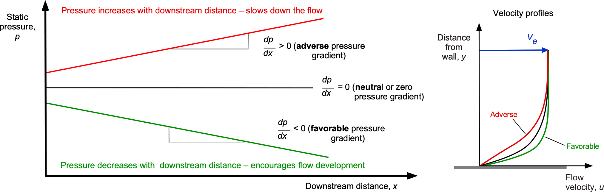
1. A pressure gradient where the pressure  decreases with increasing downstream distance, say
  , i.e., the pressure gradient is
  . This gradient is called a favorable pressure gradient because it has favorable effects on the boundary layer development, i.e., it tends to encourage the downstream development of the boundary layer and prevent it from separating from the surface.
2. A neutral or “zero” pressure gradient where  , i.e., no pressure changes with downstream distance.
3. A pressure gradient where the pressure increases with increasing downstream distance, i.e.,  . This gradient is called an adverse pressure gradient because it has adverse effects on the development of the boundary layer; i.e., the pressure forces act to retard the development of the boundary layer and thus tend to slow it down. If the pressure gradient is sufficiently adverse, it will eventually cause the boundary layer to slow down to zero near the surface and separate from the surface.
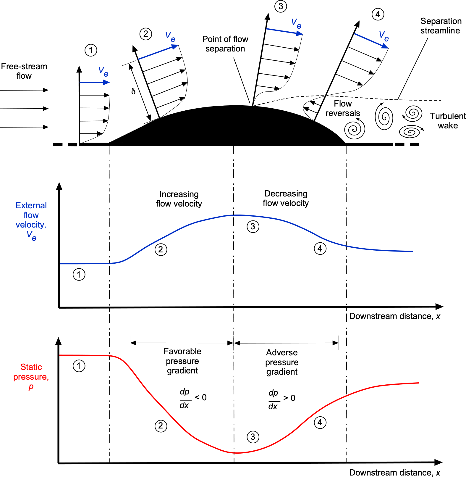
The figure below shows an example of a boundary layer flow development over a convex hump. The external flow velocity (in this case identified by the edge velocity ) increases over the front of the hump and reduces again over the back. As the flow velocity increases, its static pressure decreases (i.e., from the Bernoulli equation), and as the velocity decreases again, the pressure increases. Consequently, the corresponding pressure gradients are favorable over the front ( is negative, decreasing with distance) and adverse over the back (
 is positive, increasing with distance). The favorable pressure gradient over the front half keeps the boundary layer attached. Still, the adverse pressure gradient over the back half slows down the boundary layer flow, especially near the surface, and causes it to separate. Notice that when flow separation occurs, the flow velocity and static pressure do not immediately recover to the freestream values.
The consequence of the preceding observations is that the flow no longer easily follows the body’s contour when the gradient  , i.e., what happens when the pressure gradient is adverse and tries to slow down the flow? There comes a point where the boundary layer profile develops a point of inflection, so the corresponding shear stress becomes zero. The flow reverses, and a region of recirculating flow develops. It is said that the flow has separated, and the point where the shear stress is zero is called the flow separation point. The formal criterion for the onset of flow separation is that
(18) 
This means the flow will separate from the surface when the wall shear becomes zero. While this criterion is strictly valid only for a steady flow, it represents a quantifiable condition for predicting or identifying the onset of flow separation in a boundary layer.
It is possible to deduce that turbulent boundary layers are generally less susceptible to flow separation than a laminar boundary layer, all external influences being equal. This outcome occurs because a turbulent boundary layer has a higher flow velocity near the wall than a laminar boundary layer; therefore, it takes a longer downstream distance for the flow to approach the conditions at the wall that are likely to produce flow separation.
Summary of Boundary Layer Characteristics
The preceding observations about the boundary layer can now be summarized:
1. The flow velocity profile and other boundary layer characteristics, such as its thickness, affect the shear stresses in the fluid and the surface shear or skin friction. Hence, the boundary layer affects the drag of the surface (or body) over which it develops.
2. The characteristics of the boundary layer depend on the Reynolds number. At higher Reynolds numbers, where inertial effects in the flow are much stronger than viscous effects, boundary layers tend to be relatively thin and robust to the extent that they stay attached to surfaces for longer downstream distances. However, at lower Reynolds numbers, the boundary layers are slower and thicker and so more easily prone to separation.
3. The characteristics of the boundary layer are affected by the pressure gradients over the surface on which it develops. For example, if the surface is curved rather than flat, the flow velocities and static pressures will change along it. If the pressure gradient is sufficiently unfavorable or adverse, the boundary layer may detach or separate from the surface, a process called flow separation.
4. Most boundary layers will eventually become susceptible to separation from the surfaces over which they develop, especially after they develop over longer downstream distances. The onset of flow separation has deleterious effects on the aerodynamics of airfoils and wings, including a loss of lift and an increase in drag. Other effects, such as surface roughness and flow heating, may also significantly affect the development of the boundary layer.
Flow Separation on an Airfoil
Boundary layer separation from a body, such as an airfoil section, can have significant consequences, including a large increase in drag and a substantial loss of lift. This outcome is because the rear part of an airfoil creates an adverse pressure gradient, as shown in the figure below, which becomes increasingly adverse with an increasing angle of attack. While pressure is a scalar quantity, in this form of presentation, the pressure is plotted as a vector in a direction perpendicular to the surface of the airfoil, with lower-than-ambient static pressure areas pointing outward and higher-than-ambient pressure areas pointing inward.
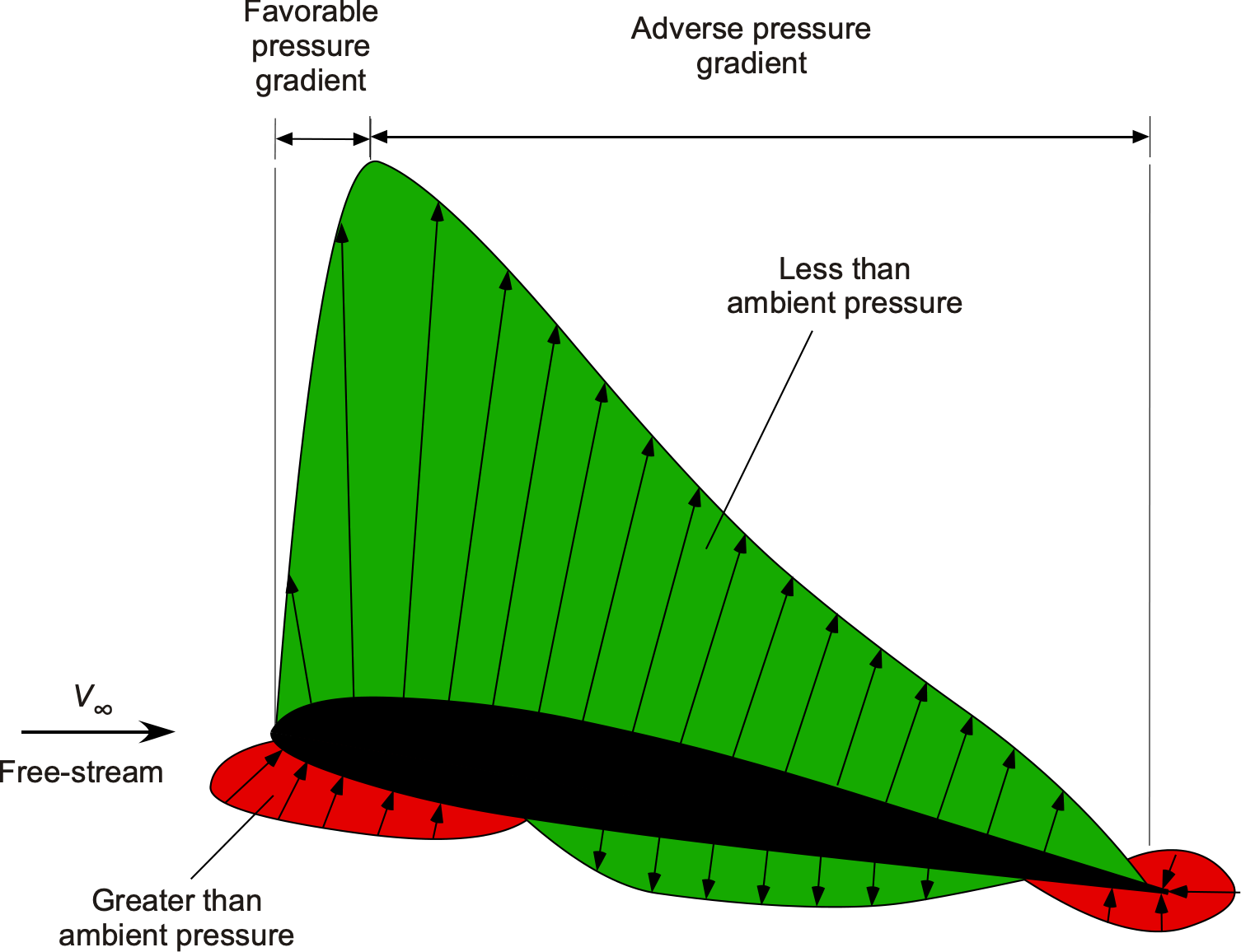
Over the front part of the airfoil, a favorable pressure gradient exists, which encourages the boundary layer to develop normally in the downstream direction. Indeed, the boundary layer may remain laminar during this time, although much depends on the surface roughness. Beyond the point of minimum pressure, an adverse pressure gradient exists over the airfoil, causing the boundary layer to transition into turbulence. Then, the subsequent development of the boundary layer begins to slow in the downstream direction as it develops in the adverse pressure gradient.
The boundary layer can withstand this gradient at low angles of attack, reaching the airfoil’s trailing edge or separating just before that point, as shown in the figure below. However, as the angle of attack increases, the more severe adverse pressure gradients cause the flow to separate at a shorter downstream distance, so the separation point moves forward. Eventually, flow separation occurs near the leading edge, and under these conditions, the airfoil is said to be stalled.
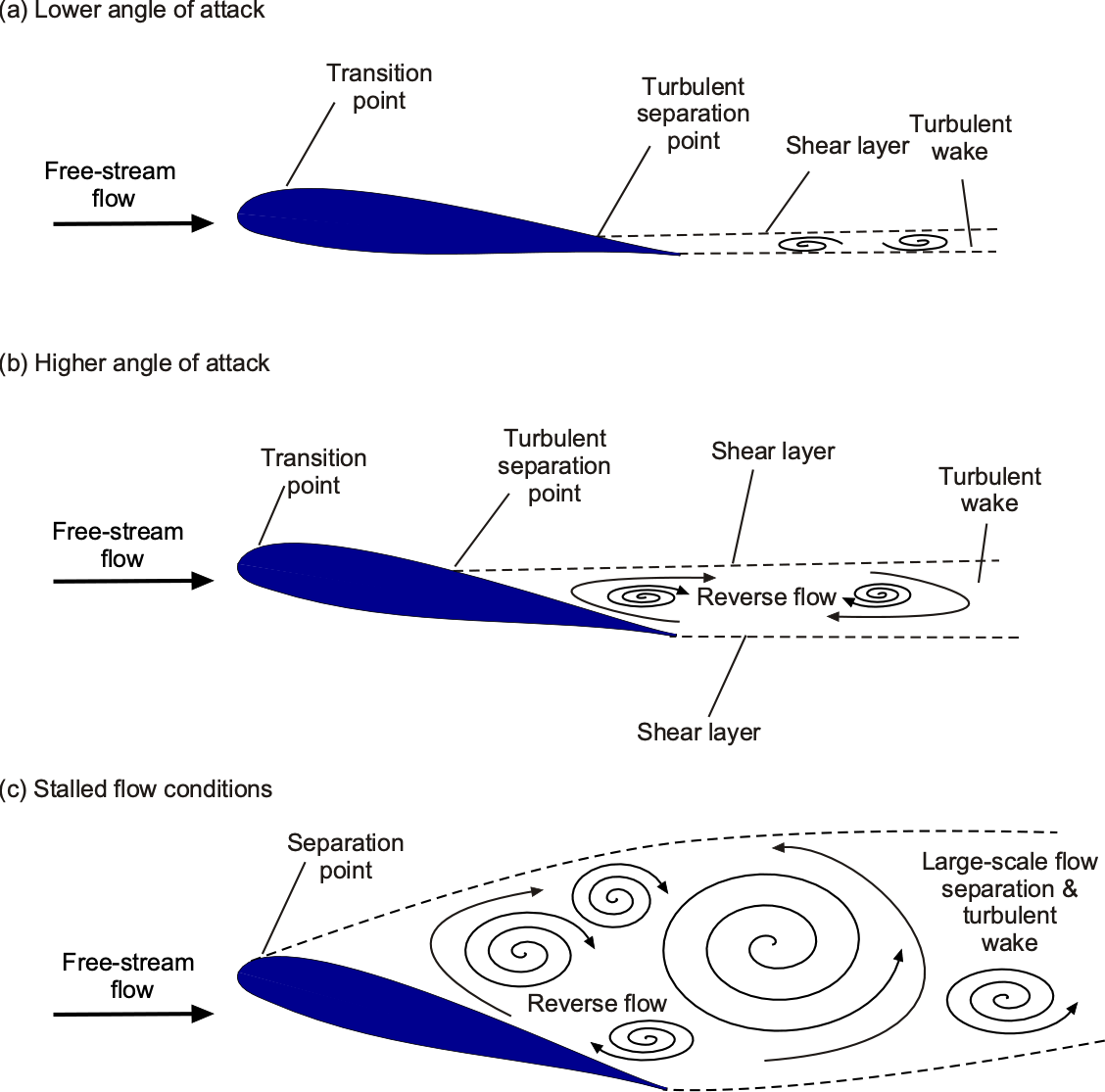
The turbulence produced in the separated flow region and wake is also a source of unsteady aerodynamic loads and buffeting on the wing. Indeed, a characteristic of stalling the wing of an aircraft during flight is the creation of unsteady aerodynamic loads and buffeting transmitted to the airframe, warning the pilot of an impending wing stall.
Boundary Layer Equations
The “boundary layer equations” are a subset of the full Navier-Stokes equations, which, in principle, are more straightforward (but not easy) to solve, partly because they are cast into a two-dimensional form using order-of-magnitude approximations. Such approximations require careful justification by comparing the resulting approximate solutions with the complete solutions (if those can be obtained), flow measurements, or sometimes with both. Experience using the boundary layer equations has shown their validity for problems bounded by the assumptions and limitations from which they were derived. For example, using the boundary layer equations to solve for the viscous flow over an airfoil at low to moderate angles of attack (below stall) has been well-proven.
Many practical problems can also be solved by using a hybrid or coupled method that combines essentially inviscid methods (e.g., potential flow methods, such as panel methods for the outer flow) with a boundary layer approach for the inner, near-surface flow, which are sometimes referred to as inviscid/viscous interaction methods. In this approach, the boundary layer solution is coupled to the inviscid solution through a specific type of boundary condition, typically in the form of a displacement thickness of the boundary layer, which provides a “virtual” airfoil shape over which the inviscid solution can be obtained. Such approaches can provide reasonable predictions of the resulting flow at a minimal cost compared to a complete Navier-Stokes solution using computational fluid dynamics (CFD).
Momentum Equations
Different approaches can be used to obtain the boundary layer equations. The most intuitive approach is to start with the incompressible form of the momentum equations and to apply them to a problem (such as the flow over an airfoil at lower angles of attack) where the boundary layer development can be assumed to be very thin (e.g., what would be obtained with a flow at higher chord Reynolds numbers). The streamline curvature is low, i.e., the streamlines are not bent by much, so the slope of the streamlines,  , remains small.
The incompressible form of the momentum (Navier-Stokes) equations can be written in a rather elegant and compact form as
(19) 
where  is the vector Laplacian of the velocity field. The equations are also often written in the form
(20) 
Expanding out the substantial derivative on the left-hand side gives
(21) 
The meaning of the terms in these equations should be appreciated, i.e.,
(22) 
The terms refer to normal compressive stresses, such as pressure, and viscous shear. Note that the normal compressive stresses in terms of the bulk viscosity do not appear in the incompressible form of the equations.
These equations can also be expanded in terms of their scalar components, giving
(23) ![\begin{eqnarray*} \mbox{${x}$ component:} \quad \quad \varrho \left(\frac{\partial u}{\partial t} + u \frac{\partial u}{\partial x} + v \frac{\partial u}{\partial y} + w \frac{\partial u}{\partial z}\right) & = & -\frac{\partial p}{\partial x} + \mu \left(\frac{\partial^2 u}{\partial x^2} + \frac{\partial^2 u}{\partial y^2} + \frac{\partial^2 u}{\partial z^2}\right) \\[8pt] \mbox{${y}$ component:} \quad \quad \varrho \left(\frac{\partial v}{\partial t} + u \frac{\partial v}{\partial x} + v \frac{\partial v}{\partial y}+ w \frac{\partial v}{\partial z}\right) & = & -\frac{\partial p}{\partial y} + \mu \left(\frac{\partial^2 v}{\partial x^2} + \frac{\partial^2 v}{\partial y^2} + \frac{\partial^2 v}{\partial z^2}\right) \\[8pt] \mbox{${z}$ component:} \quad \quad \varrho \left(\frac{\partial w}{\partial t} + u \frac{\partial w}{\partial x} + v \frac{\partial w}{\partial y}+ w \frac{\partial w}{\partial z}\right) & = & -\frac{\partial p}{\partial z} + \mu \left(\frac{\partial^2 w}{\partial x^2} + \frac{\partial^2 w}{\partial y^2} + \frac{\partial^2 w}{\partial z^2}\right) \end{eqnarray*}](https://eaglepubs.erau.edu/app/uploads/quicklatex/quicklatex.com-fc5649d9e7f1f8a1f1a6270d7f67f935_l3.svg "Rendered by QuickLaTeX.com")
Two-Dimensional, Steady Flow
For a two-dimensional flow (assumed in the – plane), there are just two scalar components, i.e.,
(24) ![\begin{eqnarray*} \varrho \left(\frac{\partial u}{\partial t} + u \frac{\partial u}{\partial x} + v \frac{\partial u}{\partial y}\right) & = & -\frac{\partial p}{\partial x} + \mu \left(\frac{\partial^2 u}{\partial x^2} + \frac{\partial^2 u}{\partial y^2} \right) \\[8pt] \varrho \left(\frac{\partial v}{\partial t} + u \frac{\partial v}{\partial x} + v \frac{\partial v}{\partial y}\right) & = & -\frac{\partial p}{\partial y} + \mu \left(\frac{\partial^2 v}{\partial x^2} + \frac{\partial^2 v}{\partial y^2} \right) \\ \end{eqnarray*}](https://eaglepubs.erau.edu/app/uploads/quicklatex/quicklatex.com-51c637c05c48c473dfdd8288e4d80923_l3.svg "Rendered by QuickLaTeX.com")
Expanding out the first and last set of terms in each case gives
(25) ![\begin{eqnarray*} \varrho \, \frac{\partial u}{\partial t} + \varrho u \frac{\partial u}{\partial x} + \varrho v \frac{\partial u}{\partial y} & = & -\frac{\partial p}{\partial x} + \mu \frac{\partial^2 u}{\partial x^2} + \mu \frac{\partial^2 u}{\partial y^2} \\[8pt] \varrho \, \frac{\partial v}{\partial t} + \varrho u \frac{\partial v}{\partial x} + \varrho v \frac{\partial v}{\partial y} & = & -\frac{\partial p}{\partial y} + \mu \frac{\partial^2 v}{\partial x^2} + \mu \frac{\partial^2 v}{\partial y^2} \\ \end{eqnarray*}](https://eaglepubs.erau.edu/app/uploads/quicklatex/quicklatex.com-780efbcd9fe667f63ca783a8173c1c03_l3.svg "Rendered by QuickLaTeX.com")
and assuming steady flow, then
(26) ![\begin{eqnarray*} \varrho u \frac{\partial u}{\partial x} + \varrho v \frac{\partial u}{\partial y} & = & -\frac{\partial p}{\partial x} + \mu \frac{\partial^2 u}{\partial x^2} + \mu \frac{\partial^2 u}{\partial y^2} \\[8pt] \varrho u \frac{\partial v}{\partial x} + \varrho v \frac{\partial v}{\partial y} & = & -\frac{\partial p}{\partial y} + \mu \frac{\partial^2 v}{\partial x^2} + \mu \frac{\partial^2 v}{\partial y^2} \\ \end{eqnarray*}](https://eaglepubs.erau.edu/app/uploads/quicklatex/quicklatex.com-4673b64ad1c6cacae4ae408bde3bc8cb_l3.svg "Rendered by QuickLaTeX.com")
Simplifications
If the boundary layer is thin compared to the dimensions of the problem (i.e., for an airfoil  where
where  is the chord) and also that the streamline curvature is slight (i.e., small such than
  ), then each of the corresponding terms in these two latter equations can be examined and perform an expected relative magnitude comparison.
- For the first convective term:
(27) 
- For the second convective term:
(28) 
- For the first viscous stress term:
(29) 
- For the second viscous stress term:
(30) 
In other words, all the terms in the component of momentum are more important than the corresponding terms in the component. It is reasonable to conclude, in this case, therefore, that
(31) 
i.e., the pressure gradients normal to the surface of the airfoil will be much weaker than the pressure gradients along the airfoil’s chord. Indeed, it is reasonable to conclude that for a thin boundary layer that develops over the surface of an airfoil, in the boundary layer that
(32) 
This outcome means that the pressure gradient (normal to the surface) within the boundary layer can be neglected, a result also verified experimentally for low-speed (subsonic) flows. This assumption, however, is not such a good one for high-speed flows where significant compressibility effects are present.
This latter result is significant because it reveals two key points. First, the local static pressure in the flow will only be a function of (not and ), hence simplifying the solution. Second, the local static pressure about the body or airfoil will not depend on the boundary layer. The pressure depends on the external flow field above the boundary layer (essentially inviscid), i.e., it will only depend on the edge velocity, , and the corresponding pressure,  . Finally, if the streamline curvature is low, then the viscous stresses from the gradients will also be low, so that
(33) 
and so these terms can also be neglected.
Thin-Layer Boundary Layer Equations
Therefore, the reduced or simplified form of the Navier-Stokes equations under these thin-layer boundary layer assumptions becomes
(34) ![\begin{eqnarray*} \varrho \, u \frac{\partial u}{\partial x} + \varrho \, v \frac{\partial u}{\partial y} & = & -\frac{d p_e}{d x} + \mu \frac{\partial^2 u}{\partial y^2} \\[8pt] \frac{\partial p}{\partial y} & = & 0 \end{eqnarray*}](https://eaglepubs.erau.edu/app/uploads/quicklatex/quicklatex.com-783ba12bfc77384ce1e44e710547912c_l3.svg "Rendered by QuickLaTeX.com")
where the  term has been replaced by
  in that the pressure now depends only on that in the direction and the external pressure, , at that. The pressure is related to the flow velocity using the Bernoulli equation (actually the unintegrated form using Euler’s equation, i.e.,
  ) so that
(35) 
Therefore, these latter equations are usually written in the form
(36) ![\begin{eqnarray*} \varrho \, u \frac{\partial u}{\partial x} + \varrho \, v \frac{\partial u}{\partial y} & = & \varrho \, V_e \frac{d V_e}{d x} + \mu \frac{\partial^2 u}{\partial y^2} \\[8pt] \frac{\partial p}{\partial y} & = & 0 \end{eqnarray*}](https://eaglepubs.erau.edu/app/uploads/quicklatex/quicklatex.com-bdbeb5358d6256b24fb9acce3929ecf5_l3.svg "Rendered by QuickLaTeX.com")
and with the addition of the conservation of mass (continuity) equation, i.e.,
(37) 
they are collectively called the incompressible form of the boundary layer equations. If time dependence is included, then
(38) ![\begin{eqnarray*} \varrho \left( \frac{\partial u}{\partial t} + u \frac{\partial u}{\partial x} + v \frac{\partial u}{\partial y} \right) & = & \varrho \, V_e \frac{d V_e}{d x} + \mu \frac{\partial^2 u}{\partial y^2} \\[8pt] \frac{\partial p}{\partial y} & = & 0 \\[8pt] \frac{\partial u}{\partial x} + \frac{\partial v}{\partial y} & = & 0 \end{eqnarray*}](https://eaglepubs.erau.edu/app/uploads/quicklatex/quicklatex.com-2360bbe5db5dc3bf3577952f15e43106_l3.svg "Rendered by QuickLaTeX.com")
These latter equations apply to all incompressible boundary layers, whether laminar, turbulent, or transitional. However, they do not apply to flows separated from the surface, such as those on stalled airfoils or in the wakes behind bluff bodies, such as circular cylinders.
In practice, although the boundary layer equations are a significantly reduced subset of the Navier-Stokes equations, they remain challenging to solve because they are a set of nonlinear equations, with the nonlinearity arising from the convective acceleration terms. Therefore, they are typically solved using numerical methods, such as finite-difference approaches, but exact solutions may be possible in some cases. The equations must be solved in all cases by specifying initial and boundary conditions.
Laminar Boundary Layer – The Blasius Solution
A classic solution in this latter category is the Blasius solution[2] for the laminar boundary layer development over a flat plate in a zero pressure gradient, which has become a classic exemplar in fluid dynamics and an essential check case for CFD and measurement methods. As shown in the figure below, the flow away from the plate has a uniform velocity of  . The downstream distance is measured in terms of , and the plate’s leading edge is at = 0. At the leading edge, there is a stagnation point. The boundary layer develops from zero thickness at that point and gets thicker, moving further downstream along the plate. This problem had been studied experimentally in the laboratory by the time Blasius tackled the theoretical solution, so Blasius had some additional physical insight into the problem that influenced the development of his theory.
Boundary Layer Equations in Zero Pressure Gradient
The boundary layer equations in a zero-pressure gradient are
(39) 
(40) ![\begin{eqnarray*} u \frac{\partial u}{\partial x} + v \frac{\partial u}{\partial y} & = & \nu \frac{\partial^2 u}{\partial x^2} \\[10pt] \frac{\partial p}{\partial y} & = & 0 \label{two} \\[10pt] \frac{\partial u}{\partial x} + \frac{\partial v}{\partial y} & = & 0 \label{three} \end{eqnarray*}](https://eaglepubs.erau.edu/app/uploads/quicklatex/quicklatex.com-22d50ee1dc233919ce8207f250cf8c74_l3.svg "Rendered by QuickLaTeX.com")
Notice that the first of the set (Eq. 40) is in terms of the kinematic viscosity  , i.e.,
  . These latter equations are sometimes known as Prandtl’s equations because Prandtl was the first to cast the more general momentum equations into this simplified form.
Stream Function & Boundary Conditions
To solve these equations for the flow field in the boundary layer, a set of boundary conditions is needed, which, in this case, are: 1. The no-slip condition at the surface, i.e.,  at
at  . 2. The conditions at infinity (a uniform flow in this case), i.e.,
  as
as  . Using the stream function,
  , is a useful way to reduce the number of variables, and Blasius employed this approach in his analysis of the boundary layer problem. His goal was to reduce the governing partial differential equations (which, in this case, are expressed in terms of and ) to a single ordinary differential equation for a single transformed variable. Remember that in terms of the stream function, , the velocity components are
(41) 
Notice that the continuity equation is automatically satisfied, i.e.,
(42) 
Equation 40 now becomes
(43) 
which is now a new governing equation. It is important to note that the mathematical definitions of the physical boundary conditions will also change. 1. The no-slip boundary condition becomes  at . 2. The boundary conditions at infinity now become
  as .
as .
Similarity Solution
Blasius’s next step was to express the solution for the velocity in the boundary layer as a self-similar solution, i.e., where the boundary layer profile can be consistently scaled as a function of downstream distance. Blasius examined the measurements of the boundary layer profile for different downstream distances, , when plotted in terms of  versus , with representing the thickness of the boundary layer. The results proved to be self-similar, which means that the velocity profile at any value of is a scaled version of the velocity profile at any other distance . When the velocity profiles were plotted as versus
  , they all collapsed into a single profile, indicating that they exhibited self-similarity when expressed in terms of these quantities.
George Stokes had already shown that for a boundary layer, the flow velocity at a distance from the surface would depend on  , the kinematic viscosity , and the distance from the leading edge of the plate , and the boundary layer thickness, , grew according to
(44) 
Dividing both sides by , then
(45) 
so the developing thickness of the boundary layer becomes a function of the Reynolds number based on downstream distance, i.e.,
(46) 
Solution of the Velocity Profile
The primary goal remains, however, which is to determine the actual theoretical shape of the boundary layer profile that will satisfy the governing boundary layer equation to find as a function of , i.e.,
(47) 
where is the desired functional relationship. From this point, Blasius defined a transformed variable,  , as
, as
(48) 
so that now
(49) 
A stream function is then defined as
(50) 
In terms of the transformed variable, then
(51) 
and
(52) 
The governing equation, i.e., Eq. 43, now becomes
(53) 
(54) 
The boundary conditions in terms of the transformed variables become  as
as  , i.e., the no-slip boundary condition, and
  as
as  , i.e., the conditions at infinity, as summarized in the table below.
| Physical coordinate | Similarity coordinates |
|---|---|
| = 0 at = 0 |
 = 0 at = 0 = 0 at = 0 |
| = 0 at = 0 |
= 0 at = 0 |
 = 0 as = 0 as |
= 1 as |
Notice that the transformed governing equation, i.e., Eq. 54, is still a third-order nonlinear differential equation, but it is now an ordinary differential equation, which is easier to solve. Therefore, Blasius’s approach converted a system of two partial differential equations into one ordinary differential equation. However, solving Eq. 54 for the function still cannot be done in closed form and requires a numerical method for which several approaches are possible. Blasius did this using a Taylor series expansion for which the coefficients of the series were numerically derived using recursive relationships, and much of his dissertation work is about finding this numerical solution.
However, other numerical methods can also be used to solve the equation. For example, the third-order ODE in Eq. 54 can be converted into a system of first-order ODEs by letting
(55) 
Therefore, the original Blasius equation in Eq. 54 now becomes
(56) 
so, the system of three ODEs to be solved are
(57) 
Also, the new initial conditions are
(58) 
This system of ODEs can now be integrated numerically (e.g., using a Runge-Kutta method) from to a sufficiently large value of , such as  , which would be well outside of the boundary layer thickness. Paul Blasius would surely have appreciated the benefits of MATLAB and the ode45 function. The initial guess is that
  is an approximate value based on known solutions; however, any other reasonable starting value can also be used.
MATLAB code to solve the Blasius equation
Show code/hide code.
% Define the Blasius equation as an equivalent ODE system
function dydeta = blasiusODE(eta, y)
f = y(1);
g = y(2);
h = y(3);
dydeta = [g; h; -0.5 * f * h];
end
% Boundary conditions
eta_max = 10;
initial_guess = 0.332; % Initial guess for h(0)
% Define the range of eta
eta_range = [0 eta_max];
% Initial conditions [f(0), f'(0), f”(0)]
initial_conditions = [0, 0, initial_guess];
% Solve the ODE using ode45
[eta, y] = ode45(@blasiusODE, eta_range, initial_conditions);
% Extract the solution
f = y(:,1);
g = y(:,2);
% Plot the results
figure;
plot(eta, g, ‘-b’, ‘DisplayName’, ‘f”(\eta)’);
hold on;
plot(eta, f, ‘-r’, ‘DisplayName’, ‘f(\eta)’);
xlabel(‘\eta’);
ylabel(‘f, f”’);
legend;
title(‘Solution to the Blasius Equation’);
grid on;
hold off;
The table below gives selected numerical values of the similarity function and its derivatives along the plate carried out until  approaches 1, i.e., the edge of the boundary layer. The value of the second derivative,
  , is needed to calculate skin friction on the surface of the plate from the action of the boundary layer.
|
|
|
|
| 0.0 | 0.0 | 0.0 | 0.332 |
| 0.5 | 0.042 | 0.166 | 0.331 |
| 1.0 | 0.166 | 0.330 | 0.323 |
| 1.5 | 0.370 | 0.487 | 0.303 |
| 2.0 | 0.650 | 0.630 | 0.267 |
| 2.5 | 0.996 | 0.751 | 0.271 |
| 3.0 | 1.397 | 0.846 | 0.161 |
| 3.5 | 1.838 | 0.913 | 0.108 |
| 4.0 | 2.306 | 0.956 | 0.064 |
| 4.5 | 2.790 | 0.980 | 0.034 |
| 5.0 | 3.283 | 0.992 | 0.016 |
| 5.5 | 3.781 | 9,997 | 0.007 |
| 6.0 | 4.280 | 0.999 | 0.002 |
 |
|
1.0 | 0.0 |
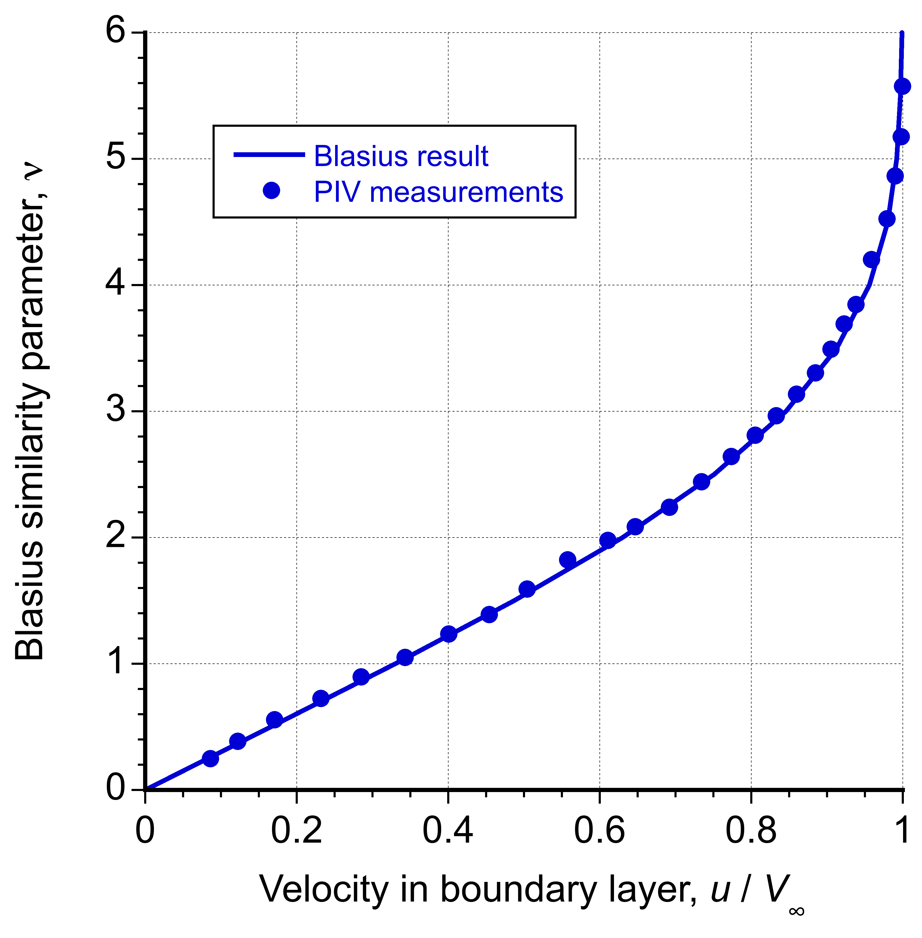
Finally, notice that the velocity profile of the laminar boundary layer is just
(59) 
which is the result Blasius set out to obtain in the very beginning. This velocity profile is plotted below. Measurements have shown that the Blasius solution to the velocity profile is in excellent agreement with measurements, which, in this case, were made using particle image velocimetry (PIV). Quod erat demonstrandum.
Other Boundary Layer Characteristics
From this result, other information about the characteristics of the boundary layer can be determined, including the boundary layer thickness and the shear stress on the wall. The boundary layer thickness, , is defined as the value of for which the velocity in the boundary layer approaches 99% of the freestream value. From the Blasius solution, this condition is obtained for = 5 so that
(60) 
or in terms of  , where
  is the Reynolds number based on “,” which is the distance from the plate’s leading edge, then
(61) 
The displacement thickness, , is obtained by integrating over the velocity profile, i.e.,
(62) ![\begin{eqnarray*} \delta^{\mbox{*}} (x) & = & \int_0^\delta \left( 1 - \frac{u}{V_{\infty}} \right) dy \\[8pt] & = & \left(\frac{\nu x}{V_e} \right)^{1/2} \int_0^{\infty} \left( 1 - f^{\prime} \right) d \eta \\[8pt] & = & \left(\frac{\nu x}{V_e} \right)^{1/2} \lim_{\eta \rightarrow \infty} \left( \eta - f \right) \\[8pt] \end{eqnarray*}](https://eaglepubs.erau.edu/app/uploads/quicklatex/quicklatex.com-332a26e758ae75e7a701b32adc98752b_l3.svg "Rendered by QuickLaTeX.com")
giving
(63) 
where 1.721 is found from the numerical solution. Therefore, the quantity can be written as
(64) 
Also, the momentum thickness, , is
(65) 
or
(66) 
It will be apparent that the values of and can be expressed in terms of the boundary layer thickness, i.e.,
(67) 
and
(68) 
The shear stress on the surface (the wall stress) is
(69) 
and from the tabulated numerical values given previously then  = 0.332. Therefore,
(70) 
As already discussed, it is often preferred to use non-dimensional forms of quantities in aerodynamics, e.g., lift coefficient, drag coefficient, and the like. When dealing with boundary layers, a local non-dimensional shear stress coefficient or skin friction coefficient  is used, which is defined in terms of the freestream dynamic pressure as
(71) 
The value of will be a local quantity because it will vary from point to point across the surface, so the value of will also vary.
The local skin friction coefficient is used with integration to calculate the total drag on an exposed surface from the action of the boundary layer. The drag on a plate of finite length  would be given by integrating the value of the local skin friction along the length of both sides of the plate, i.e.,
(72) 
For an airfoil section of chord , then
(73) 
This latter result is often used as a benchmark in that it would represent the absolute minimum drag on a thin airfoil if the flow developed along its length in a fully laminar manner. Therefore, an ideal goal would be to design for laminar flow, but one that is never practically attainable because the flow will always become turbulent at any practical flight Reynolds number.
Extensions of the basic approach used by Blasius (i.e., similarity solutions) have been made by various authors, including the work of Faulkner & and Skan, who generalized the boundary layer solutions for various external velocity fields and hence allowed for the effects of pressure gradients. However, these laminar solutions tend to be more of academic interest than any actual practical use because the boundary layers on most flight vehicles are inevitably turbulent.
Turbulent Boundary Layers
The principles surrounding the development of a turbulent boundary layer, which is distinctive because this type of flow has more mixing between the fluid layers and a more uniform velocity profile, have already been discussed and shown in the figure below. Recall also that a turbulent boundary layer will be thicker than a laminar one, a point previously made, because of the larger extent of mixing in the flow. However, expressing the structure of a turbulent boundary layer is much more complicated mathematically, and there are no theoretical results like the Blasius solution.
A turbulent boundary layer has been well-studied experimentally, but developing a generalized, functional relationship for the velocity profile remains challenging. However, various approximations for the turbulent boundary layer profile can be used. Among the simplest and the best-known approximations is the power-law profile, which is expressed as
(74) 
where the value of  is a constant that depends on the Reynolds number. It is found that the value of tends to increase with increasing Reynolds number to give agreement with measured profiles of turbulent boundary layers. However, using
  for many flows is sufficient to represent a turbulent boundary layer profile called the “one-seventh power law,” as shown in the figure below.
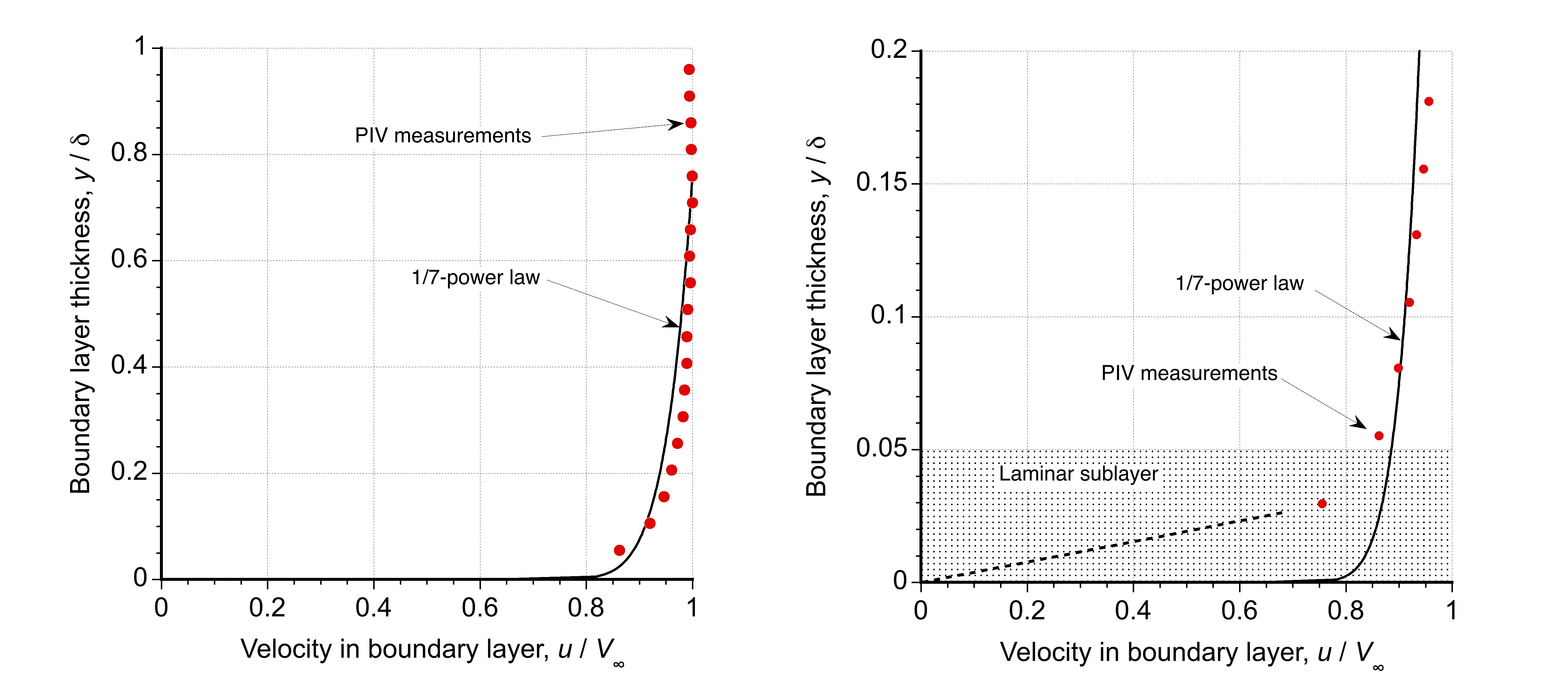
However, a disadvantage of the power-law profile is that it cannot be used to calculate the shear stress precisely at the wall (i.e., at ) in the laminar sublayer because it gives an infinite velocity gradient there. Notice that the laminar sublayer is a thin layer at the wall where the flow is predominantly smooth and may be regarded as a region where varies linearly with , i.e.,
(75) 
where  is the thickness of the laminar sublayer. Understanding the laminar sublayer is essential in analyzing turbulent boundary layer flows and must be considered when studying heat transfer and drag forces.
For a turbulent boundary layer development along a flat plate, the boundary layer thickness can be approximated by
(76) 
This preceding relationship assumes that the flow is turbulent right from the start of its development and that the velocity profiles are self-similar along with the flow in the x-direction. Neither of these assumptions is true for the general turbulent boundary layer case, so care must be exercised when applying this formula to any problems.
Check Your Understanding #2 – Skin Friction from laminar & turbulent boundary layers
Consider two boundary layer profiles at a wall, one laminar and one turbulent. The laminar profile is given by  and the turbulent profile by
  where is the edge velocity (external velocity) and is the boundary layer thickness. Calculate the shear stress on the wall in each case where for the turbulent boundary layer is twice that of the laminar boundary layer and explain why they differ.
Show solution/hide solution.
The shear stress, , on the wall in each case is given by
![\[ \tau_w = \mu \left( \frac{du}{dy} \right) = \mu \left(\frac{V_e}{\delta} \right) \left( \frac{d (u/V_e)}{d (y/\delta)} \right)~\mbox{ as $(y/\delta)\rightarrow 0$} \]](https://eaglepubs.erau.edu/app/uploads/quicklatex/quicklatex.com-aa18a2f2a66dcaaea48f418d327e823a_l3.svg "Rendered by QuickLaTeX.com")
So, for the laminar boundary layer.
![\[ \frac{d (u/V_e)}{d (y/\delta)} = 2 \left(1 - (y/\delta) \right) = 2~\mbox{ as $(y/\delta)\rightarrow 0$} \]](https://eaglepubs.erau.edu/app/uploads/quicklatex/quicklatex.com-854fac31754590bf52645f99002195fe_l3.svg "Rendered by QuickLaTeX.com")
and for the turbulent boundary layer
![\[ \frac{d (u/V_e)}{d (y/\delta)} = (1/7) (y/\delta)^{-6/7} = 53.25~\mbox{ as $(y/\delta)\rightarrow 0.001$} \]](https://eaglepubs.erau.edu/app/uploads/quicklatex/quicklatex.com-4a46e9d42a437a713ae9c4acd36fd5d5_l3.svg "Rendered by QuickLaTeX.com")
In the latter case, the gradient has been evaluated at a short distance from the wall because the gradient would otherwise become infinite as  0. If for the turbulent boundary layer is twice that of the laminar boundary layer, the latter value will be reduced by about 1.81 to 29.39.
It is clear then that the turbulent boundary layer produces a much higher skin friction coefficient on the wall for given values of and . Hence, it will also have a much higher drag on a body over which such a boundary layer may exist.
Visualizing the Boundary Layer
Boundary layers are typically very thin regions next to a surface, so they are challenging to visualize using measurement techniques. Nevertheless, standard flow visualization methods in the wind tunnel environment can reveal the signature and perhaps specific boundary layer properties. Flow visualization may be divided into surface flow visualization and off-the-surface visualization. Such methods include but are not limited to, smoke or other tracer particles, tufts, surface oil flows, liquid crystals, sublimating chemicals, pressure-sensitive paints, shadowgraph, schlieren, etc.
An example illustrating the effects of the two boundary layer states on an airfoil at a low angle of attack and relatively low Reynolds number is shown in the figure below. In this case, the flow was visualized in a wind tunnel using a surface oil flow technique in which light oil is applied to the surface with a brush and illuminated under an ultra-violet (UV-A) light source. The shear stress on the oil mixture from the boundary layer creates a pattern, with regions of lower skin friction leaving behind more significant oil accumulations.
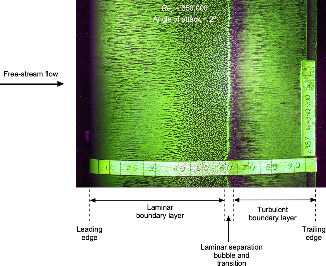
For these conditions, the forward 60% of the airfoil can be interpreted to have a laminar boundary layer; the low surface shear stress here allows the oil to accumulate, especially near the mid-chord where the boundary layer approaches the transition point. Downstream of the transition, the boundary layer state is fully turbulent, with higher shear stresses causing more of the oil on the surface to be removed. Notice that the transition region is short where the flow is separated, indicative of a laminar separation bubble. However, it must be remembered that what is observed on the surface does not always indicate what is happening in the external flow.
Fun experiment – thanks for listening to a boundary layer!
How can you listen to a boundary layer? Well, it turns out that is easier than you think! It is necessary to have some pressure taps in the surface connected to a piece of rubber tubing. In the wind tunnel, a particular type of tubing called Tygon is used. You can plug it into your ear on the other end of the tube, much like a physician uses a stethoscope. You will soon be able to hear the differences!
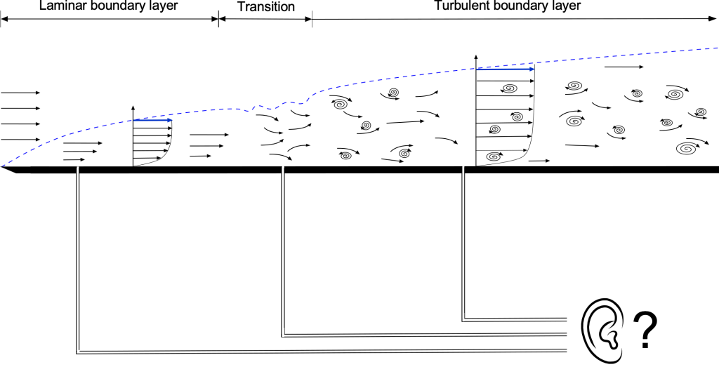
You will hear little for a smooth laminar flow over the surface, except for a light swishing noise. For a fully turbulent flow, you will hear much more of a rumbling noise because of the unsteady pressure disturbances caused by turbulence. Finally, you will hear bursts of swishing and rumbling for a transitional flow. Fascinating!
Skin Friction Drag on an Airfoil
Estimating the skin friction drag on bodies with a turbulent boundary layer is an essential problem in aerospace engineering. While the situation is generally complex for a complete airplane or other flight vehicles because of the complex surfaces and the highly three-dimensional boundary layers that subsequently develop, the process can be illustrated for a two-dimensional airfoil. An airfoil is reasonably thin and flat, so at least at low angles of attack, a flat plate can be used to approximate the shape and drag on an airfoil.
The net shear stress drag on the plate with the laminar flow can be found by integrating the local shear along the plate’s length or the chord . For the Blasius result, then the sectional drag coefficient is
(77) 
where the factor “2” is needed because the plate has upper and lower surfaces; this latter result is plotted for reference in the figure below.
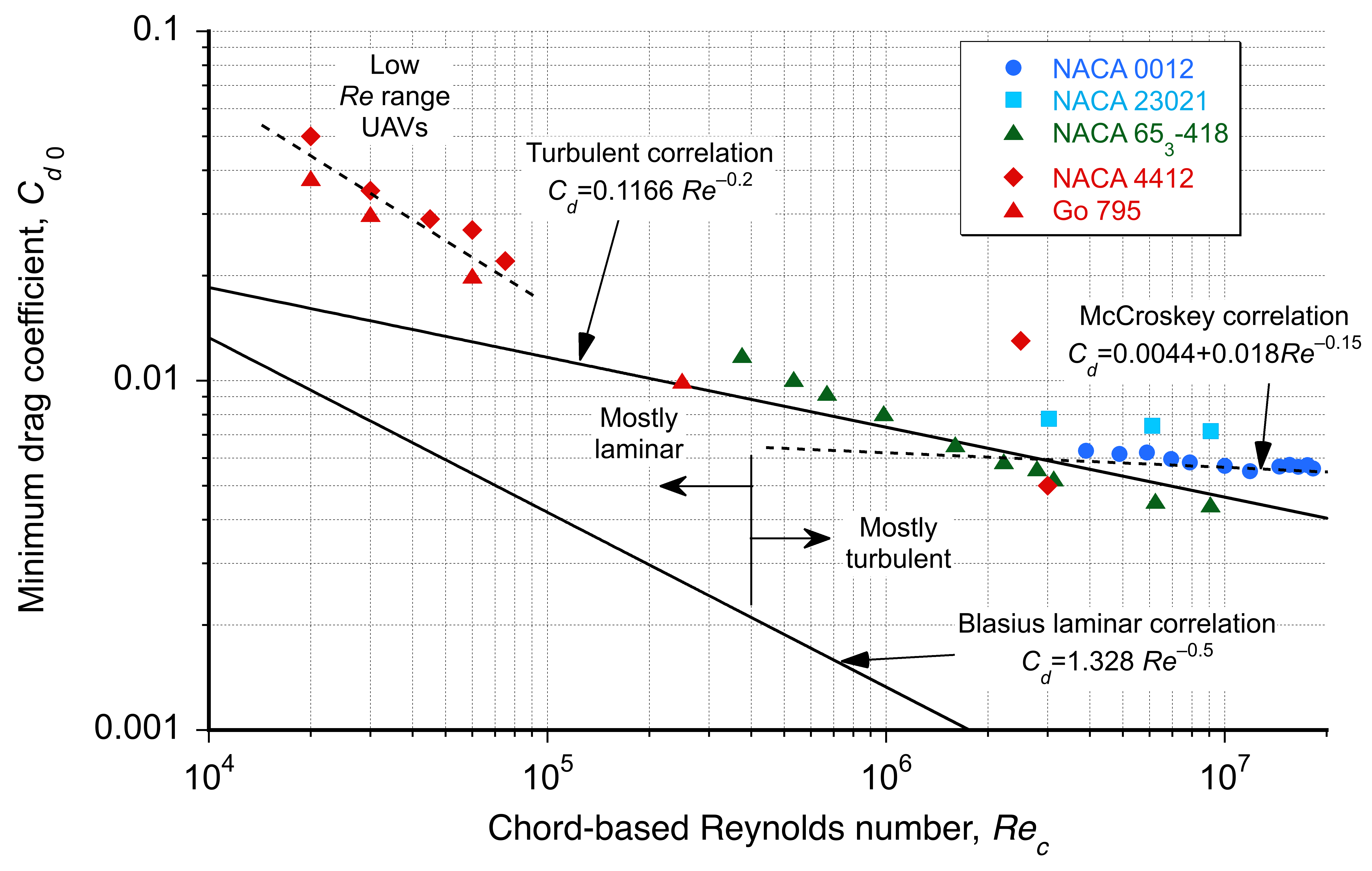
For the fully turbulent boundary layer development on a flat plate, the skin friction coefficient  on one side of the plate is found to conform to an empirical relationship given by
(78) 
This latter result is obtained by assuming the velocity profile corresponds to a 1/7th power law profile, as given previously. If the plate was to have a fully turbulent boundary layer over its upper and lower surfaces, then by integration (as for the laminar case), it is found that
(79) 
where  is the chord-based Reynolds number. The validity of the latter expression is generally limited to a range between
  and
and  . Below
  , the boundary layer can generally be assumed to be laminar, that is, unless the pressure gradients are particularly adverse, which will slow the flow near the wall and cause the boundary layer to separate, perhaps forming a laminar separation bubble.
The results shown in the graph above suggest that the turbulent flat-plate solution is a good approximation to the viscous (shear) drag on many airfoils over a fairly wide range of practical Reynolds numbers found during flight on aircraft, i.e., for above  . In this case, it will be sufficient to assume that
(80) 
where  is the reference chord Reynolds number for which a reference value of drag
  is known for a given airfoil section; not all airfoils will have known (measured) drag coefficients at all Reynolds numbers, but this approach allows the drag coefficient for other Reynolds numbers to be estimated with good confidence.
The empirical drag equation, which McCroskey has suggested for practical use, is
(81) 
offers an improved correlation at the higher chord Reynolds numbers, which will be typical of those found on larger aircraft and at higher flight speeds. The laminar boundary layer separates more readily at very low Reynolds numbers, below  . The drag coefficients of typical airfoils are larger than either laminar or turbulent boundary layer theory would suggest.
Airfoil behavior in this Reynolds number regime is essential for many classes of small-scale air vehicles, i.e., UAVs. In this case, it can be seen in the above figure relating drag coefficient to Reynolds number that changing the scaling coefficient from  0.2 to 0.4 in Eq. 80 gives a good approximation (line fit) based on the results shown over a lower range of . However, the drag of airfoils in this regime tends to be less predictable, especially at other than shallow angles of attack, because the boundary layers are thicker, often with laminar separation bubbles, and the onset of flow separation occurs more readily.
Laminar Separation Bubbles
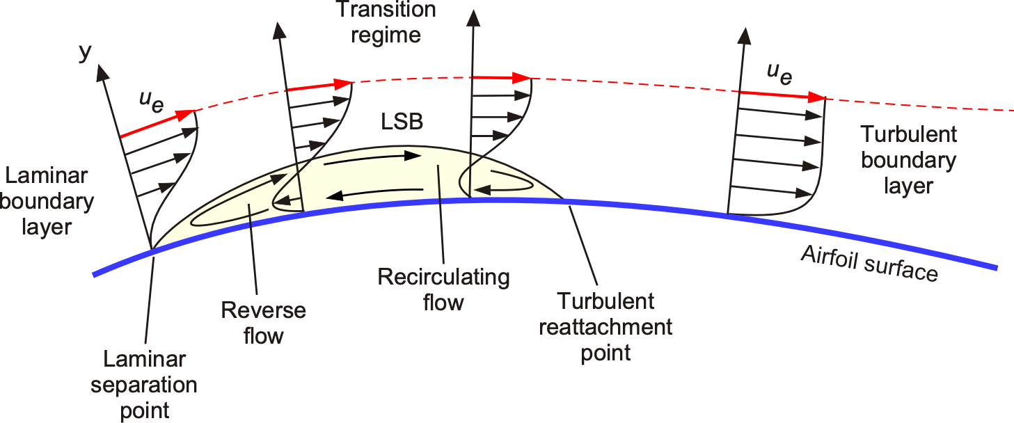
The name “laminar separation bubble” has been mentioned previously, but what is it? A laminar separation bubble, or LSB, is often found on airfoil sections and at many chord Reynolds numbers. However, they are usually longer and more pronounced on airfoil sections operating at lower Reynolds numbers below 10 .
.
The figure below shows a schematic of an LSB. Laminar separation bubbles occur as the initial boundary layer approaches the point of laminar separation, which is at or immediately downstream of the leading edge pressure (suction) peak on an airfoil. After laminar separation occurs, the flow will temporarily leave the airfoil surface but undergo a transition process and immediately reattach as a turbulent boundary layer. It does this because a turbulent boundary layer can more easily withstand a given adverse pressure gradient than a laminar boundary layer. The result is a region (usually relatively small at higher chord Reynolds numbers) of recirculating separated flow of content pressure. At lower Reynolds numbers, a long LSB may be formed. LSBs can also be observed by a slight constant pressure region when the chordwise pressure distribution is measured near the airfoil’s leading edge. With surface oil flow visualization, as previously discussed, the LSB is evidenced by an accumulation of oil.
Effects of Surface Roughness
The development of a boundary layer is profoundly affected by pressure gradients and surface roughness. For example, the transition from a laminar to a turbulent boundary layer flow is often caused prematurely by the effects of surface roughness, as shown in the figure below, which acts to enhance the mixing of the flow in the lower layers of the boundary layer and so to produce turbulence more quickly. However, it should be appreciated that a laminar boundary layer is so thin that it takes only a tiny amount of roughness to initiate the transition process. Leading edge roughness on an airfoil will inevitably eliminate any laminar separation bubbles.
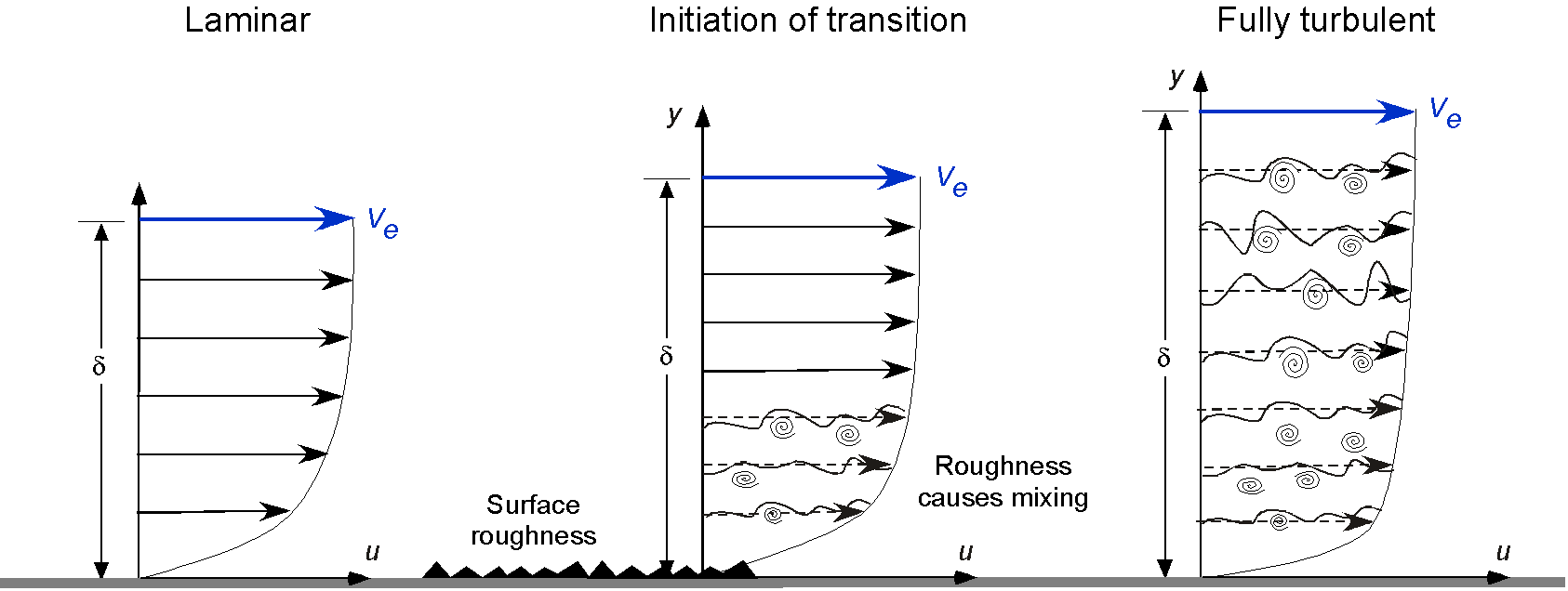
As this turbulence develops near the surface, it mixes up through the higher layers in the boundary layer. As a result, it quickly progresses through the entire boundary layer from top to bottom, except immediately near the wall. Surface roughness can be present on a surface for various reasons, including just the “in-service” use of an aircraft, such as average abrasion at the leading edge of a wing, which will increase the drag of that wing. However, in some cases, such as with golf balls, surface roughness can have beneficial effects; the transition to a turbulent boundary layer delays flow separation and reduces the pressure drag on the ball.
Boundary Layer Flow Control
Much ongoing research is into “laminar” flow wings and active flow control technology to improve aerodynamic efficiency. Control over the natural turbulent boundary layer that forms on an aircraft by keeping it laminar could reduce skin friction drag. Such an approach could minimize aircraft drag by up to an order of magnitude and significantly reduce fuel consumption, especially for high-speed aircraft.
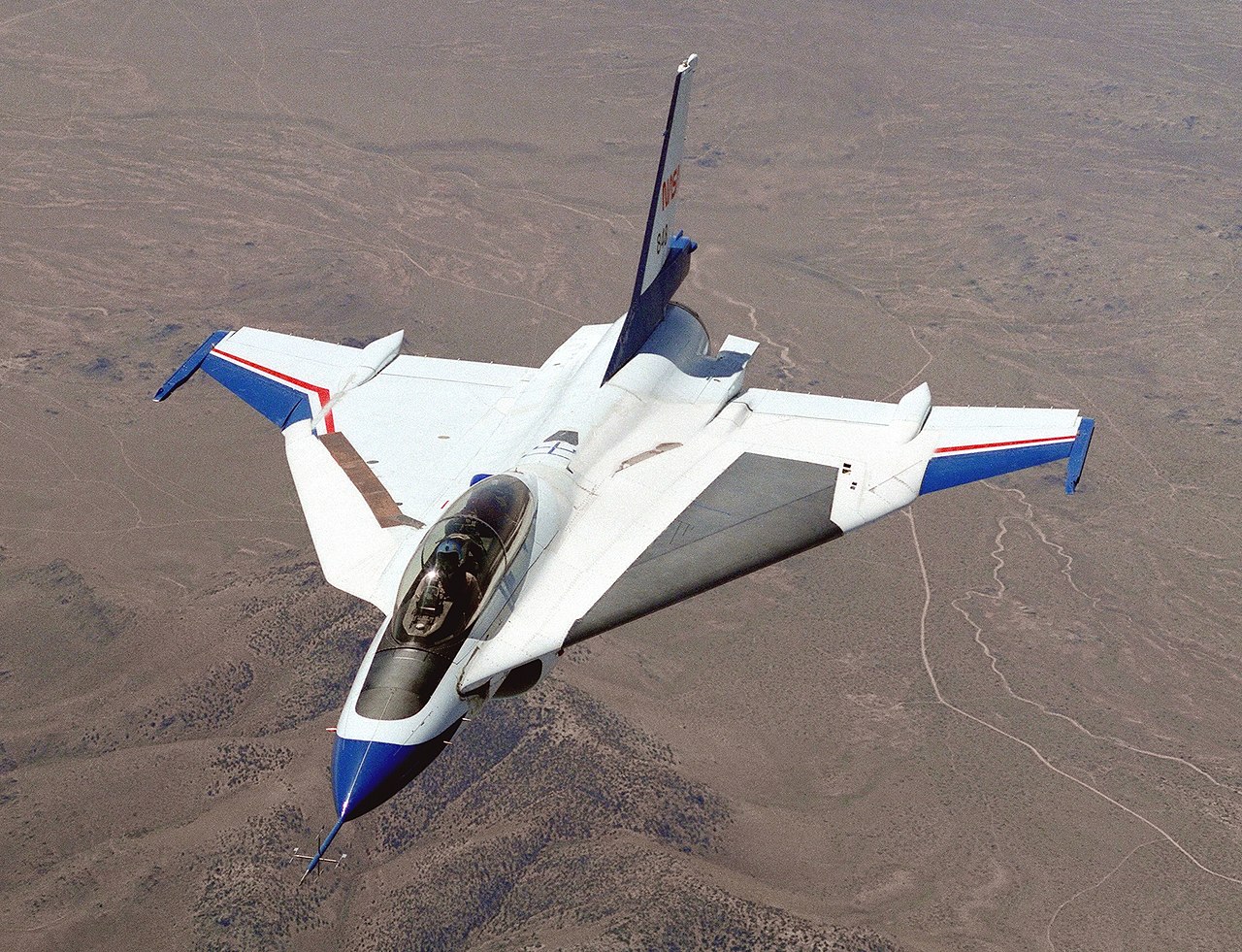
NASA has tested a modified F-16 with a porous glove over the wing, as shown in the photograph below. The glove is the black region on the left wing. The glove contained over 10 million tiny holes drilled by lasers and connected to a suction system. This approach removed a portion of the slower part of the boundary layer close to the surface, extending the laminar flow region across the wing. However, there are many challenges in developing practical boundary layer control systems for aircraft, including weight, reliability, maintainability, and costs.
Thermal Boundary Layers
A thermal boundary layer is a concept used in fluid dynamics and heat transfer to describe the region near a surface where the temperature of the fluid changes rapidly from the temperature at the surface (the wall) to the temperature of the external bulk fluid flow. Heat is transferred when a fluid flows over a wall with a temperature different from that of the fluid. This heat transfer process creates a region adjacent to the wall, known as the thermal boundary layer , where the temperature gradient is significant.
Heat Transfer
Assume that a flow with freestream temperature  starts to flow over a wall with a higher temperature
  , i.e.,
  . At the hotter wall, the flow velocity is low and approaches the no-slip condition at the surface, as shown in the figure below. Because there is a temperature difference between the wall and the flow, heat is first transferred across the wall/fluid interface and into the fluid by thermal conduction. Heat is then progressively transferred away from the wall by thermal convection into successive layers of fluid until, at some distance from the wall, the temperature approaches the bulk flow temperature. The distance at which
  is called the thermal thickness,
  . The rate at which the thermal boundary layer grows differs from the viscous or velocity boundary layer. If the freestream temperature is higher than the surface temperature, i.e.,
  , heat can be transferred to the surface by means of thermal convection. In particular, turbulent boundary layers can carry heat to the surface.
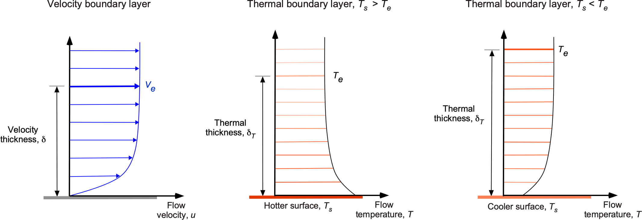
The rate of heat conductive transfer from the wall per unit area, also known as heat flux (which has units of energy per unit time per unit area), depends on the temperature gradient at the wall, often called Fourier’s law. In its one-dimensional form, it is expressed as
(82) 
where  is known as the thermal conductivity of the fluid (which has units of energy per unit time per length per unit temperature). The minus sign indicates that heat flows in the opposite direction of the temperature gradient from higher to lower, i.e., in accordance with the second law of thermodynamics. The value of the thermal conductivity, , depends on the type of fluid and its temperature, and is a measured quantity derived from heat transfer experiments.
Nusselt Number
The heat transfer per unit area of the wall can also be expressed in terms of Newton’s law of cooling, i.e.,
(83) 
where, in this case,  is the convective heat transfer coefficient (expressed on units of energy per unit time per unit area per unit temperature), a value that can also be found from experiments. Because the conductive heat transfer is transferred as convection into the thermal boundary layer, equating Eqs. 82 and 83 gives
(84) 
This latter relationship in Eq. 84 can be non-dimensionalized by using
(85) 
and
(86) 
where is some characteristic length. Therefore, after some additional steps, then it can be shown that
(87) 
which is a dimensionless temperature gradient, the dimensionless grouping  being known as the Nusselt number, i.e,
(88) 
Recall that is the conductive thermal transfer of the fluid, and is the convective transfer, so the physical interpretation of the Nusselt number becomes apparent. In the case of a thermal boundary layer, the reference length for the Nusselt number can be taken as the thermal thickness, .
Prandtl Number
In the study of thermal boundary layers, the Prandtl number,  , is often used, which is a dimensionless similarity parameter defined as the ratio of viscous or “momentum” diffusivity to thermal diffusivity, i.e.
(89) 
where  is the thermal diffusivity, which is the heat transfer rate from one point to another, and
  is the specific heat at a constant pressure. The product
  is called the volumetric heat capacity, i.e., the ability of the fluid to absorb and store thermal energy. The momentum diffusivity, normally called kinematic viscosity, is a measure of the fluid’s resistance to shear relative to its density.
Therefore, it will be apparent that the physical significance of the Prandtl number is a relative measure of convective heat transfer relative to conductive heat transfer. For  , thermal diffusivity is more important, and for
  , momentum diffusivity is more important. Notice that the Prandtl number has no length scale, and its value depends solely on the temperature-driven values of the fluid parameters. Its value and other properties, such as density, viscosity, and thermal conductivity, are usually listed.
For gases, then  , e.g., for the laminar flow of air,
  , which means that thermal diffusivity is more important than viscous diffusion, so
  . Values of the Prandtl number depend on the fluid and whether it is laminar or turbulent. In the case of a turbulent flow, it is often assumed that
  for air, but this value will depend on the turbulence levels in the flow. For liquids
  , e.g., for water at ambient temperature conditions, then
  , and for more viscous fluids such as oils, then
  .
.
The thickness of the thermal boundary layer, , depends on factors such as the flow velocity, specific fluid properties, and the surface temperature. Generally, a thicker thermal boundary layer will have slower heat transfer rates, while a thinner boundary layer allows for quicker heat transfer between the wall and the fluid. Turbulence enhances heat transfer by mixing the fluid near the surface more effectively, bringing more lower-temperature fluid into contact with the hot surface, thereby increasing the thermal gradient and the overall heat transfer rate. Therefore, it will also be apparent that the Prandtl number is related to the velocity boundary layer and thermal boundary layer by
(90) 
Importance of Thermal Boundary Layers
Understanding thermal boundary layers is critical for high-speed flight vehicles to manage aerodynamic heating, select structural materials, and ensure structural integrity. Supersonic and hypersonic flight generate intense aerodynamic heating from compressibility and wall shear. Thermal boundary layers form around the aircraft’s surfaces from this heating, affecting the distribution of temperatures and the thermal stresses experienced by the aircraft structure. For example, the leading edges of Concorde reached temperatures over 130oC, which is enough to begin to change the material properties of conventional aluminum; to this end, special high-temperature “Hiduminium” alloy had to be used. Metals are also very good at conducting heat, so the entire airframe reached relatively high temperatures, which caused it to expand thermally, which was as much as 0.5 ft (0.15 m) from nose to tail. To this end, many parts of the internal structure used pin-jointed and/or sliding elements to alleviate the stresses.
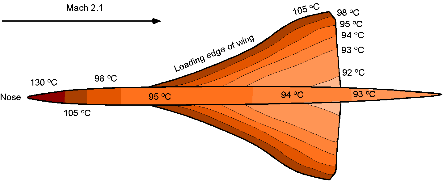
During re-entry into Earth’s atmosphere or when entering the atmospheres of other planets, spacecraft encounter intense heat generation from friction with the atmosphere. Understanding thermal boundary layers is crucial for designing effective heat shields to efficiently dissipate heat and prevent the spacecraft from burning up during re-entry. Heat shields are usually made of an ablative material that breaks down, and pieces are shed off into the flow in layers, enhancing heat transfer. Spacecraft may utilize other thermal protection systems consisting of silica tiles, ceramics, and other coatings that can withstand high temperatures. These systems often rely on the principles underlying the behavior of thermal boundary layers to dissipate heat efficiently and protect the spacecraft’s structure and components.
The surface temperatures of the Space Shuttle, as shown in the figure below, reached temperatures of 1,300 K during the re-entry at Mach = 14. Because the atmosphere is so thin during the initial stages of re-entry, the Reynolds numbers are low and the boundary layer over a spacecraft is naturally predominantly laminar at this flight condition, which provides a thin layer of cooler insulating flow to keep the surface of the vehicle at a lower temperature. In this flight, a boundary layer trip was placed on the lower surface of the port wing downstream of the leading edge to create and study the effects of turbulence; the subsequent higher temperature zone (in red) suggests that disturbed turbulent flow causes the surface temperatures to increase significantly. Therefore, maintaining laminar flow as long as possible during re-entry is crucial for reducing thermal loads and ensuring the effectiveness of the thermal protection system. This goal is achieved through aerodynamic design, surface characteristics, and suitable re-entry trajectories.
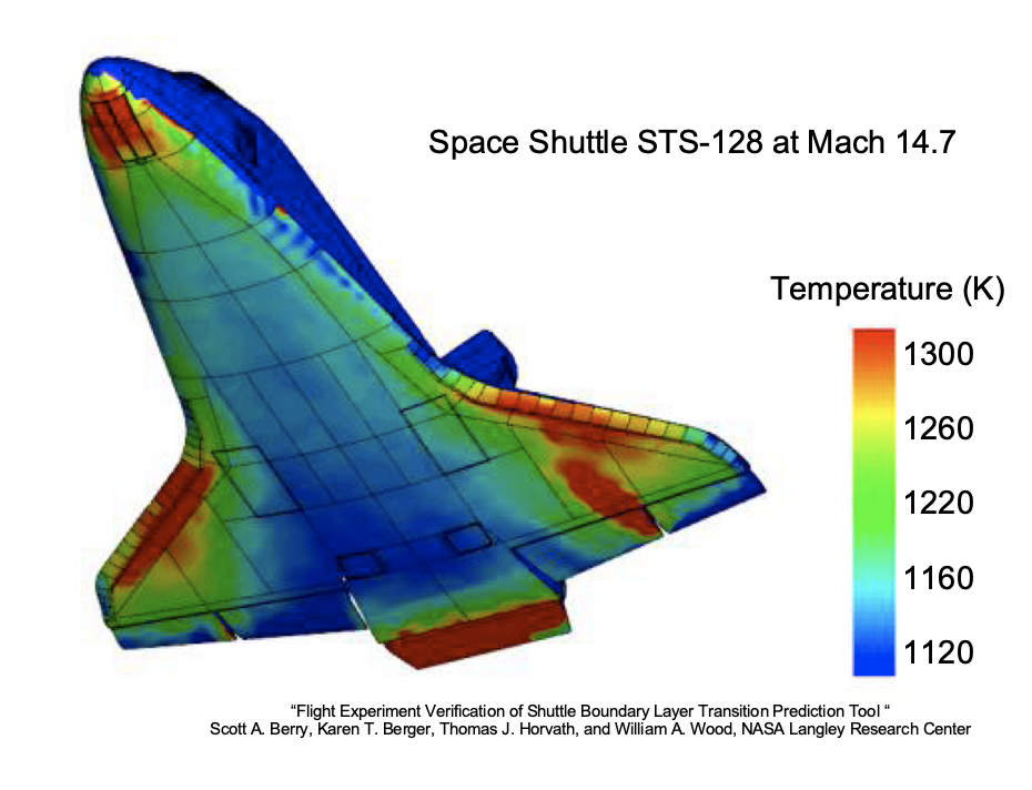
Summary & Closure
- Becker, John, V., "Boundary-Layer Transition on the NACA 0012 and 23012 Airfoils in the 8-Foot High-Speed Wind Tunnel," Special Report, NACA-SP-137, January 1940. ↵
- Paul Richard Heinrich Blasius, "Grenzschichten in Flgkeiten mit kleiner Reibung,'"which is usually cited in the form of the NACA translation "The Boundary Layers in Fluids With Little Friction," NACA TM-1256. ↵
