48 Aircraft Stability & Control
Introduction[1]
An aircraft’s or other flight vehicle’s stability and control characteristics are rather complicated, not just because of the relatively advanced mathematics needed to explain it. Nevertheless, the subject’s basic principles can still be introduced physically without straying too far into the mathematics. While the professional practice of stability and control requires specialist knowledge and considerable experience, it is nevertheless essential for all aerospace engineers, regardless of their primary specialization, to develop a good understanding of the fundamentals of this field, and also appreciate its primary importance in the aircraft design process.
The term “stability” in reference to a flight vehicle is the tendency for that vehicle to continue to fly in its prescribed or trimmed flight condition after being subjected to a disturbance, i.e., an aircraft is considered stable when it remains in the flight condition that the pilot intends it to be in. The term “trim” or “trimmed flight” represents the equilibrium state, where the forces and moments on the vehicle are in perfect balance. If the aircraft does something else when subjected to a disturbance, such as a gust or pilot control inputs, the aircraft would not be considered stable and could even be unstable in some unusual cases.
Most aircraft are inherently stable by design, but to a greater or lesser degree, so they can be safely flown by an average pilot without excessive control effort and workload. The term “workload” is a measure of how easy (or how difficult) the aircraft is to fly. The term “control” means the ability to change the flight attitude or other state of the flight vehicle, i.e., to make it do what is commanded. Naturally, a flight vehicle’s inherent or natural stability and the control of its flight by a pilot (or auto-pilot) are inextricably linked.
Learning Objectives
- Appreciate the fundamentals of flight vehicle stability and control, and why stability is essential for flight.
- Understand the differences between a flight vehicle’s static and dynamic stability.
- Become familiar with flight dynamic terms like short-period and long-period responses, phugoid, Dutch roll, and spiral divergence.
- Be aware of an airplane’s primary design features contributing to its static and dynamic stability characteristics.
- Know about how to assess aircraft stability and control characteristics.
- Understand what is meant by aircraft handling qualities assessments.
Forces & Moments of Flight
Following the seminal instructional work of Arthur Babister, flight dynamics concerns an aircraft’s flight characteristics and motion through the air. Stability in flight dynamics refers to the ability of an aircraft to maintain or return to a particular flight condition after being disturbed by an external force or forces. Static stability is the initial tendency of an aircraft to return to its original attitude: positive static stability means the aircraft returns to its original flight condition, and neutral static stability means it stays in the new condition. Negative static stability means it moves further away from its original condition and attitude.
Dynamic stability describes the aircraft’s behavior over time following a disturbance, which, in many cases, is an oscillatory response. For example, a disturbance in pitch may cause the dynamic response to consist of a series of nose-high and nose-down pitching motions. Positive dynamic stability means the oscillations will decrease in amplitude and return to their original condition; neutral dynamic stability means the oscillations will remain constant in amplitude; negative dynamic stability means the oscillations increase in amplitude.
The stability and overall flight dynamics of an aircraft will depend on the following fundamental sources:
1. Aerodynamic Effects
Aerodynamic forces and moments will depend on the aircraft’s angular orientation to the flow as well as its linear velocities. These are often called static forces and moments because they depend on the aircraft’s instantaneous position in three-dimensional space. In particular, an aircraft’s lift and drag forces depend on its linear velocities through the air. Aerodynamic effects are also influenced by the aircraft’s angle of attack with respect to the flight velocities, the air density, as well as the wing and empennage geometry. For high rates of change, unsteady aerodynamic effects may be significant because the instantaneous velocities may be insufficient to describe the aerodynamics fully. Therefore, to calculate the aerodynamics, what happened to the aircraft’s motion at a prior time, i.e., a hereditary effect, may be necessary to know.
2. Aerodynamic Damping Effects
Aerodynamic damping forces and moments arise from the aircraft’s angular velocities, sometimes called rotary forces and moments. Damping typically reduces the transient or oscillatory motion and is usually a desirable flight dynamic characteristic in that it contributes favorably to the aircraft’s stability. An aircraft’s wing and horizontal and vertical tail surfaces primarily contribute to the damping. For higher rates of change, apparent mass aerodynamic effects (also called added mass) may also be significant. Negative aerodynamic damping may be produced in unusual flight conditions, such as at high angles of attack with stalled flow.
3. Inertia Effects.
These effects arise from the aircraft’s mass distribution in response to linear and angular accelerations. These forces and moments are of two types: linear inertial and angular inertial effects. Linear inertial effects produce forces that arise from the aircraft’s mass in response to linear accelerations. Angular effects occur from the aircraft’s mass distribution and angular accelerations, which are governed by its moments of inertia. Higher moments of inertia are undesirable because they generally make the aircraft more “sluggish,” less agile, and sometimes more challenging to fly. In most cases, the balance between the distribution of aerodynamic and inertial forces will factor into the aircraft’s handling qualities.
4. Effects of Flight Controls
The application of flight controls can significantly affect the aircraft’s aerodynamics, which is obviously by design. Examples of flight controls are the ailerons, elevator, and rudder. These flight controls can affect the motion and stability of the aircraft in roll, pitch, and yaw. Furthermore, the flaps and slats (if any) and spoilers (if any) can affect the aircraft’s flight characteristics, particularly at low airspeeds, such as during takeoff and landing. The size and aerodynamic effectiveness of the flight control surfaces must be designed as an integral part of the stability and control assessments of the aircraft.
5. Gravitational Effects
Gravity manifests as weight (a force) and the distribution of weight, i.e., the position of the center of gravity, usually denoted by CG or c.g. or cg, the symbols often being used interchangeably. The c.g. is the point at which the aircraft’s weight can be considered to act, and it has an essential effect on the stability and control of the aircraft. If the c.g. is too far backward, the aircraft may become more challenging to fly or even unstable in pitch. At the same time, if the c.g. is too far forward, the aircraft may become excessively stable and difficult to maneuver and/or control. The fuel load, as well as passengers and cargo, need to be appropriately distributed within the design limits of the specific aircraft to ensure that its trim and stability are maintained during the entire flight, also allowing for the weight of fuel burned. Commercial airliners, for example, burn off a considerable weight fraction of fuel during flight, perhaps as much as 30% of their takeoff weight.
6. Propulsive Effects
These are the effects of the engine(s) that propel the aircraft forward. The propulsive thrust affects the aircraft’s speed, acceleration, and overall performance. The magnitude of the thrust depends on several factors, including the type and design of the engine, the power setting, and the aircraft’s speed. For example, propulsive thrust changes can produce aircraft pitching moments. For a multi-engine aircraft, losing one engine may cause the aircraft to yaw and/or pitch and/or roll, significantly affecting its flight characteristics and overall stability. Aircraft with large propellers may also have gyroscopic and slipstream effects that may influence their stability and control characteristics. Of recent significance is the issues with the Boeing 737 MAX, which features larger and more powerful engines mounted further forward on the wing, exacerbating thrust/pitch coupling effects.
7. Other Factors
Other factors influencing the flight dynamics of an aircraft are atmospheric conditions, flight altitude (i.e., density altitude), flight airspeed (i.e., true airspeed and dynamic pressure), and corresponding Mach number. These factors can all affect the aerodynamic characteristics of the aircraft and its propulsion system(s). So, they will directly or indirectly impact the aircraft’s performance, flight dynamics, and overall handling characteristics. Other factors include meeting stability and control requirements, which are not just limited to regulations. However, aircraft must also meet rigorous stability and control standards set by aviation authorities such as the FAA (Federal Aviation Administration) and EASA (European Union Aviation Safety Agency).
Stability Definitions
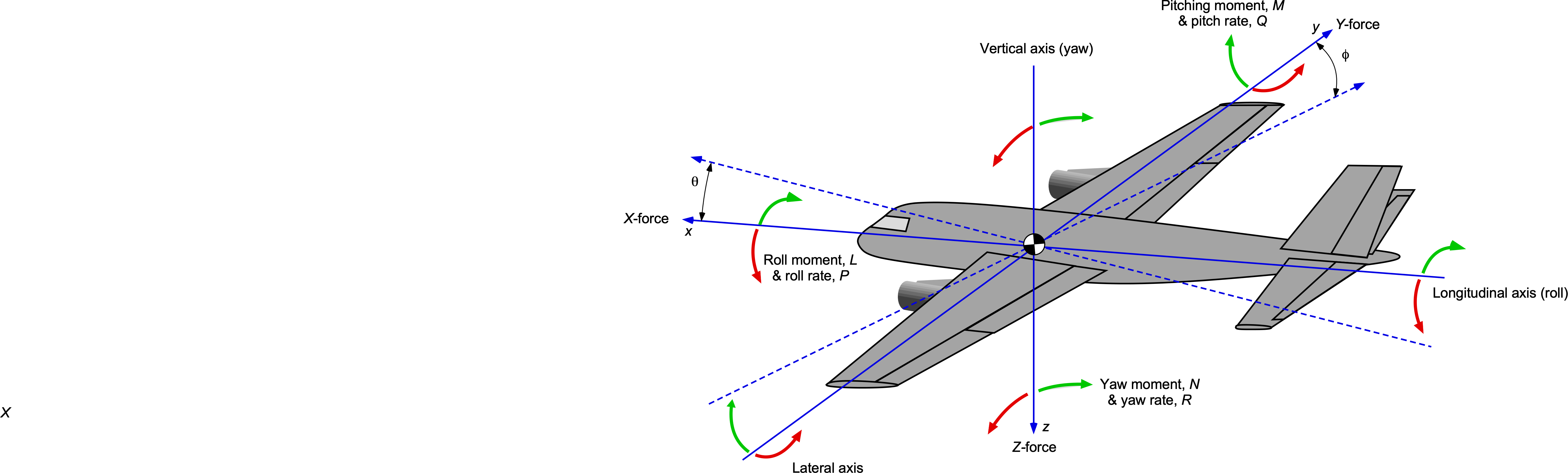
An airplane is just one type of aircraft, but its analysis forms an essential basis for understanding the dynamics and control characteristics of all flight vehicles. The issue of concern is with its stability and control characteristics about all three flight axes, as shown in the figure below, namely:
- Longitudinal stability and control concern the airplane’s response in the pitch or angle of attack degree of freedom.
- Lateral stability and control relate to the lateral axis or rolling degree of freedom.
- Directional stability and control relate to the yawing axis or directional (weathercock) degree of freedom.
While the flight responses and control inputs of any airplane tend to be coupled about the three axes to some degree, it is found in practice that its pitch or angle of attack motion is mainly decoupled from the roll and yaw responses. However, an airplane’s lateral (roll) and directional (yaw) stability characteristics tend to be significantly more coupled; usually, one cannot be considered separately from the other for a stability and control analysis.
Coordinate Systems
The airplane’s body axis is usually defined as a right-handed Cartesian coordinate system centered at the airplane’s c.g. The  direction is defined as positive along the airplane’s longitudinal axis, with positive being forward in the direction of flight. The
  direction is positive along the starboard wing, and
  is positive downward. The locations of the axes in the vertical (pitching) plane are shown in the figure below.
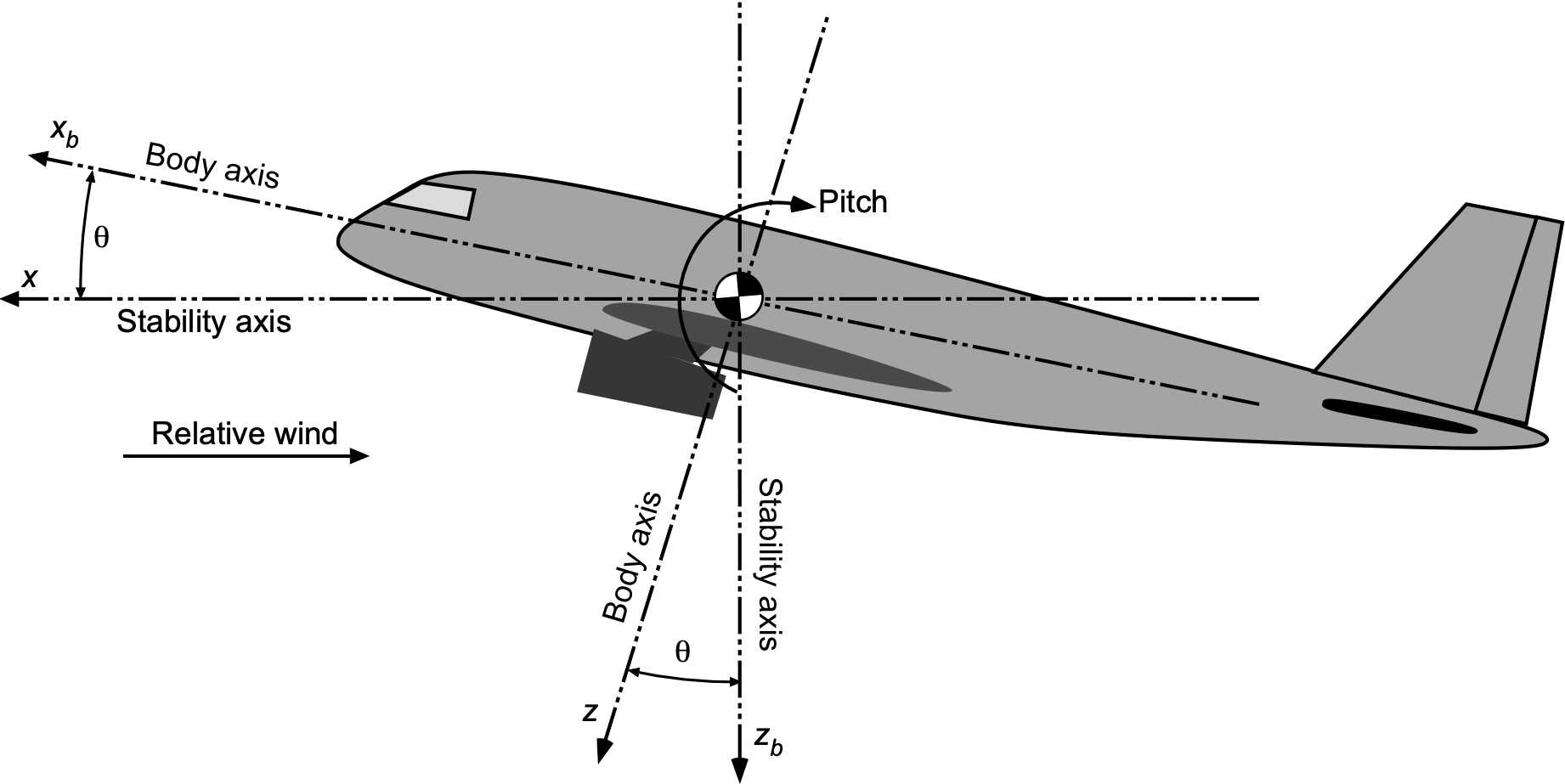
The stability coordinate system, also known as the stability axis system, is essential in flight dynamics for analyzing an aircraft’s stability and control characteristics. This system is set to align with the relative airflow and is distinct from the body axis system, which is fixed relative to the aircraft. In the stability axis system, sometimes called the wind axes, the  -axis points forward along the aircraft’s velocity vector, the
  -axis points to the right, and the
  -axis points downward. This orientation is more natural and simplifies the analysis of aerodynamic forces and moments because they are directly aligned with the airflow.
If required, the transformation from the body axis system to the stability axis system involves rotations by the angle of attack and sideslip angle. This realignment makes it easier to understand how aerodynamic forces like lift, drag, and side force act on the aircraft and how it responds. The stability coordinate system is particularly useful in deriving the equations of motion, which describe the aircraft’s response to control inputs and external disturbances. By resolving aerodynamic forces and moments in this system, engineers can more effectively analyze and ensure the aircraft’s stability and control during flight.
Attention! Potential for symbol conflict
It is essential to note the potential for symbol conflict between flight dynamic terms and aerodynamic forces and moments, which must be carefully distinguished and properly reconciled in any analysis to prevent undesirable mathematical outcomes. Flight dynamic moments, typically denoted as  ,
,  , and
, and  , representing roll, pitch, and yaw moments, respectively, can sometimes conflict with aerodynamic forces and moments which are often represented by the same symbols but with different meanings, e.g., for lift, for aerodynamic pitching moment, and for normal force. A clear and consistent notation system should be adopted to mitigate this potential for confusion. Ensuring that these symbols are distinctly defined and consistently applied throughout the analysis will help avoid misunderstandings and errors.
Trimmed Flight
For an airplane to be in static equilibrium or trim at a particular flight condition, the net sum of all the forces and moments acting on the airplane must be zero, i.e., the position and attitude of the aircraft will be in perfect balance about all three flight axes, namely pitch, roll, and yaw. The two tables below summarize the forces, moments, and velocities, one for the forces and the other for the moments.
| Axis | Force | Linear Velocity | Description |
|---|---|---|---|
|
 |
 |
Fore/aft |
|
 |
 |
Sideward |
|
 |
 |
Heave or plunge |
| Axis | Moment | Moment Coefficient | Angular Displacement | Angular Velocity | Non-dimensional angular rate | Description |
|---|---|---|---|---|---|---|
|
|
 |
 |
 |
 |
Roll |
|
|
 |
 |
 |
 |
Pitch |
|
|
 |
 |
 |
 |
Yaw/sideslip |
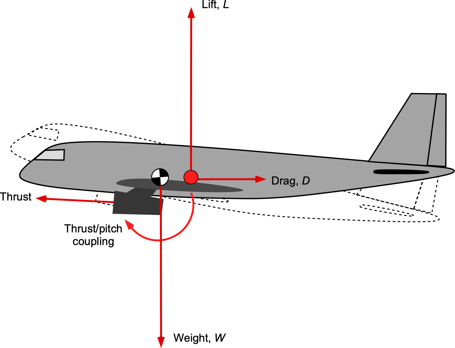
Consider the equilibrium of an airplane in straight and level unaccelerated flight at a constant airspeed and altitude, as shown in the figure below. In trim, the lift on the airplane equals its weight, and for most purposes, the weight can be considered to act at a c.g. location. The thrust (from the propulsion system) equals the aerodynamic drag at that in-flight weight, airspeed, and altitude. Therefore, as previously defined, no net forces or moments can act on the airplane about the c.g. when in the trim condition.
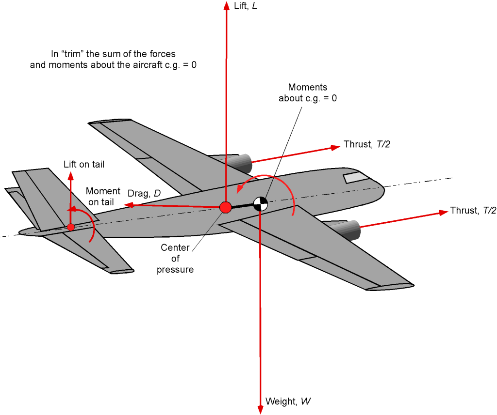
The aerodynamic forces on the airplane can be considered to act at an effective location on each lifting component, i.e., the main wings as well as the horizontal and vertical tails. Of more significance is the lifting contributions, in aggregate, which can be assumed to act at a single point. The center of pressure is a convenient point, usually denoted by CP or cp or c.p., because this location has no net aerodynamic moment. The c.g. is generally located in front of the c.p. (for stability), and the horizontal tail and flight controls are needed to create the necessary aerodynamic forces (and hence moments) to reach a balanced pitch or trimmed flight condition.
The main wing produces most of the lift on the airplane, but the tail may make some small increments. Hence, the center of pressure of the entire airplane is usually very close to the center of pressure of the wing by itself, which, for the lift coefficients typical of flight, is near the 1/4-chord point. The horizontal tail acts like a smaller version of the main wing and can give either positive or negative changes in the lift using the elevator control. Because of the typically long distance (arm) from the horizontal tail to the c.g. location (but not always), only relatively small changes in the lift on the tail are required to produce significant longitudinal pitching moments.
Trim Equilibrium Equations
For an airplane to be in static equilibrium (or in trim) at a particular flight condition, the net sum of all the forces and moments acting on the airplane must be zero. This implies that the position and attitude of the airplane will be in perfect balance about the pitch, roll, and yaw axes. In trim, the conditions for force equilibrium are
(1) 
where  represents the sum of all forces. Because there are no net forces, there will be no resultant accelerations on the airplane, which can be expressed as
(2) 
where , , and are the components of the velocity in the body-fixed frame along the , , and axes, respectively.
For rotational equilibrium, there are no net moments about the flight axes. Therefore,
(3) 
In trim, the angular velocities about the flight axes are zero, i.e.,
(4) 
where , , and are the roll, pitch, and yaw rates, respectively. For level, symmetric, coordinated flight with no yaw or sideslip, the trim conditions are
(5) 
Therefore, the airspeed component in the -direction is  , where is the true airspeed. Furthermore, if the wings are level, then the roll angle is zero, i.e.,
(6) 
Factors Affecting Trim
The trim state of an airplane, ensuring balanced steady-state flight, is influenced by multiple factors including the aircraft’s weight and center of gravity (c.g.) position, aerodynamic forces, control surface deflections, and thrust. Changes in configuration, such as flap settings and landing gear position, also impact trim, as do atmospheric conditions like air density. Additionally, fuel load and its distribution, along with external stores on military aircraft, affect the c.g. and trim. These factors collectively determine the precise adjustments needed to maintain the desired flight attitude and stability.
Flight Controls
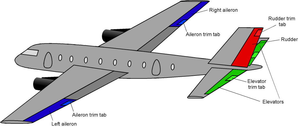
Pilot inputs and autopilot systems play a crucial role in adjusting control surfaces and engine power to maintain the desired trim state, as illustrated in the figure below. These adjustments involve precise movements of the elevator, ailerons, rudder, and thrust levels to counteract any deviations caused by changes in weight distribution, aerodynamic forces, and atmospheric conditions. Proper management of these factors ensures that the aircraft remains stable, balanced, and efficient throughout the flight, compensating for shifts in the c.g. and alterations in configuration such as flap settings and landing gear position (up/down). Small “trim tabs” are often used on the primary control surfaces to remove any residual load on the pilot’s controls so that the airplane can be flown “hands off.”
Center of Gravity Location
Consider what would happen if the center of gravity (c.g.) moved forward. In this case, a more significant nose-down gravitational moment would be produced on the airplane, which would need to be compensated for by increasing the downforce (negative lift) on the tail. Therefore, the elevator would need to be deflected up by the pilot by moving the control column aft, reducing the aerodynamic upward force on the tail and continuing to balance the net moments on the airplane to reestablish trim. Small changes in aerodynamic forces and moments from the control surfaces can be performed using trim tabs, as shown in the figure above, which can be actuated separately to trim the airplane and remove any residual forces from the pilot’s controls.
Propulsion Effects
The propulsion system can also affect the stability and control characteristics of the airplane. Propulsion will create a thrust vector, which may have a line of action that is vertically or horizontally offset from the location of the c.g. Thrust can also produce a pitching moment, i.e., a form of thrust/pitch coupling, which tends to increase the pitch attitude nose-high; this latter effect is illustrated in the figure below. Airplanes with underslung engines that produce thrust vectors centered below the c.g. are prone to this type of coupling, which can also be interpreted in combination with the airspeed coupling effect. In this latter regard, changes in thrust setting will cause changes in airspeed; increasing thrust generally increases airspeed and causes nose-up pitch, while reducing thrust decreases airspeed and can cause the nose to drop.
Center of Pressure Changes
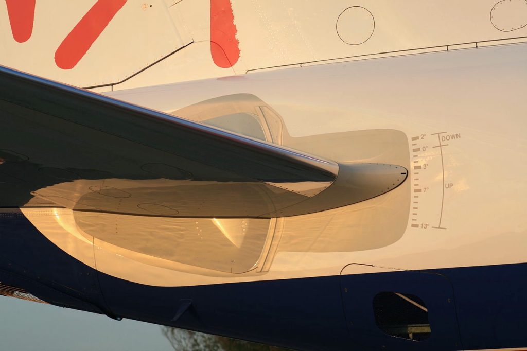
Both the c.g. and the airplane’s center of pressure (or center of lift) may, and generally will, change during flight. As fuel is burned off and the airplane’s weight changes, the c.g. may move forward or aft, depending on the type of airplane and how it is loaded with the payload. Therefore, the airplane’s stability characteristics can (and often will) change slowly during flight, and further trimming by the pilot or flight control system may be required. To reduce the trim drag on a commercial airliner, fuel is pumped from one tank to another to manage the longitudinal and lateral c.g. position during flight rather than accepting the increased drag from the application of trim tabs. As shown in the photograph below, all-flying horizontal tails may also be used on airliners to trim out the pitching moments. The markings UP and DOWN refer to the angles needed for “nose-up” trim and “nose-down” trim, respectively
The center of pressure may also change with airspeed, especially in high-speed flight at higher Mach numbers. Approaching transonic and into supersonic flight, the center of pressure typically migrates aft on the wing from near the 1/4-chord to closer to the 1/2-chord. The resulting effect is a pronounced nose-down pitching moment. This effect is called Mach tuck, and it can be a stability and control issue for a supersonic airplane as it transitions from subsonic to supersonic flight. Of course, these effects can often be trimmed out using the elevator (or a trimmable tail surface). Still, there will be a limit to this type of control capability depending on the combination of the c.g. and/or c.p. movements during flight. On some larger airplanes, it is necessary to pump fuel longitudinally from one tank to another to keep the c.g. between the required limits during supersonic flight, such as was done on the Concorde using trim tanks.
Stability Derivatives
The stability characteristics of an aircraft in response to disturbances from trimmed flight can be explained using stability derivatives, i.e., the change in a specific force or moment with respect to particular types of disturbances. To this end, it can be assumed that the forces and moments on the aircraft are functions of the instantaneous values of the disturbance velocities (translational and angular), as well as their time rates of change. Unsteady or hereditary effects (i.e., what happened in previous time) can be ignored, which is often referred to as a quasi-steady assumption.
General Representations
Therefore, the quasi-steady forces on the aircraft can be expressed in general terms as
(7) ![\begin{eqnarray*} X &= & f_X\left(u, \, \overbigdot{u}, \, v, \, \overbigdot{v}, \, w, \, \overbigdot{w}, \, p, \, \overbigdot{p}, \, q, \, \overbigdot{q}, \, r, \, \overbigdot{r} \right)\\[8pt] Y &= & f_Y\left(u, \, \overbigdot{u}, \, v, \, \overbigdot{v}, \, w, \, \overbigdot{w}, \, p, \, \overbigdot{p}, \, q, \, \overbigdot{q}, \, r, \, \overbigdot{r}\right)\\[8pt] Z &= & f_Z\left(u, \, \overbigdot{u}, \, v, \overbigdot{v}, \, w, \, \overbigdot{w}, \, p, \, \overbigdot{p}, \, q, \, \overbigdot{q}, \, r, \overbigdot{r}\right) \end{eqnarray*}](https://eaglepubs.erau.edu/app/uploads/quicklatex/quicklatex.com-bff3f2ca92c4b41e5396a97f9719de61_l3.svg "Rendered by QuickLaTeX.com")
and for the corresponding moments, then
(8) ![\begin{eqnarray*} L &= & f_L\left(u, \, \overbigdot{u}, \, v, \, \overbigdot{v}, \, w, \, \overbigdot{w}, \, p, \, \overbigdot{p}, \, q, \, \overbigdot{q}, \, r, \, \overbigdot{r}\right)\\[12pt] M &= & f_M\left(u, \, \overbigdot{u}, \, v, \, \overbigdot{v}, \, w, \, \overbigdot{w}, \, p, \, \overbigdot{p}, \, q, \, \overbigdot{q}, \, r, \, \overbigdot{r}\right)\\[12pt] N &= & f_N\left(u, \, \overbigdot{u}, \, u, \, \overbigdot{w}, \, w, \, \overbigdot{w}, \, p, \, \overbigdot{p}, \, u, \, \overbigdot{r}, \, r \right) \end{eqnarray*}](https://eaglepubs.erau.edu/app/uploads/quicklatex/quicklatex.com-6e377cf8ba23b3eef3f5fc8dc5161a04_l3.svg "Rendered by QuickLaTeX.com")
The function,  , in each case, represents the relationship between the aircraft’s instantaneous motions (or disturbances) and the resulting forces (, , and ) and the corresponding moments (, , and ) on the aircraft. With 12 dependencies in each case and potentially non-linear and interdependent (coupling) effects, it becomes clear that this is one reason why the mathematical description of the flight dynamics of an aircraft tends to become complicated.
Furthermore, if the effects of the flight control deflections,  , are added, where the subscript
  refers to the ailerons,
  refers to the elevator, and
  refers to the rudder, then there will be 18 dependencies in each case, i.e.,
(9) ![\begin{eqnarray*} X &= &f_X\left(u, \, \overbigdot{u}, \, v, \, \overbigdot{v}, \, w, \, \overbigdot{w},\, p, \overbigdot{p}, \, q, \, \overbigdot{q}, r, \, \overbigdot{r}, \, \delta_a, \, \overbigdot{\delta}_a, \, \delta_e, \, \overbigdot{\delta}_e,\, \delta_r, \, \overbigdot{\delta}_r \right)\\[8pt] Y &= &f_Y\left(u, \, \overbigdot{u}, \, v, \, \overbigdot{v}, \, w, \, \overbigdot{w},\, p, \overbigdot{p}, \, q, \, \overbigdot{q}, r, \, \overbigdot{r}, \, \delta_a, \, \overbigdot{\delta}_a, \, \delta_e, \, \overbigdot{\delta}_e,\, \delta_r, \, \overbigdot{\delta}_r \right)\\[8pt] Z &= &f_Z\left(u, \, \overbigdot{u}, \, v, \, \overbigdot{v}, \, w, \, \overbigdot{w},\, p, \overbigdot{p}, \, q, \, \overbigdot{q}, r, \, \overbigdot{r}, \, \delta_a, \, \overbigdot{\delta}_a, \, \delta_e, \, \overbigdot{\delta}_e,\, \delta_r, \, \overbigdot{\delta}_r \right)\\[8pt] L &= &f_L\left(u, \, \overbigdot{u}, \, v, \, \overbigdot{v}, \, w, \, \overbigdot{w},\, p, \overbigdot{p}, \, q, \, \overbigdot{q}, r, \, \overbigdot{r}, \, \delta_a, \, \overbigdot{\delta}_a, \, \delta_e, \, \overbigdot{\delta}_e,\, \delta_r, \, \overbigdot{\delta}_r \right)\\[8pt] M &= &f_M\left(u, \, \overbigdot{u}, \, v, \, \overbigdot{v}, \, w, \, \overbigdot{w},\, p, \overbigdot{p}, \, q, \, \overbigdot{q}, r, \, \overbigdot{r}, \, \delta_a, \, \overbigdot{\delta}_a, \, \delta_e, \, \overbigdot{\delta}_e,\, \delta_r, \, \overbigdot{\delta}_r \right)\\[8pt] N &= &f_N \left(u, \, \overbigdot{u}, \, v, \, \overbigdot{v}, \, w, \, \overbigdot{w},\, p, \overbigdot{p}, \, q, \, \overbigdot{q}, r, \, \overbigdot{r}, \, \delta_a, \, \overbigdot{\delta}_a, \, \delta_e, \, \overbigdot{\delta}_e,\, \delta_r, \, \overbigdot{\delta}_r \right) \end{eqnarray*}](https://eaglepubs.erau.edu/app/uploads/quicklatex/quicklatex.com-88536f480d9c6ee7b4d2cb889548cc89_l3.svg "Rendered by QuickLaTeX.com")
More contributions could also be added to the list, such as for the effects of flaps, engine thrust, etc, so the problem quickly becomes formidable and even intractable from any reasonable practical perspective.
Linearization Process
The method used in flight dynamics is to linearize the preceding relationships with a Taylor series expansion about the trim state and then retain only the first-order derivatives. Therefore, the perturbations to the forces and moments, i.e.,  , are now desired. The equilibrium is defined as
  , representing the balanced forces and moments on the airplane in the trimmed flight condition. For example, for the force, then
(10) ![\begin{eqnarray*} \begin{split} X_0 + \Delta X = X_0 &+ \left[\pd{X}{u} \, u + \ppd{X}{u} \, \dfrac{u^2}{2!} + \pppd{X}{u} \, \dfrac{u^3}{3!} + \ldots\right] \\[3pt] &+ \left[\pd{X}{\overbigdot{u}} \, \overbigdot{u} + \ppd{X}{\overbigdot{u}} \, \dfrac{\overbigdot{u}^2}{2!} + \pppd{X}{\overbigdot{u}} \, \dfrac{\overbigdot{u}^3}{3!} + \ldots\right] \\[3pt] &+ \left[\pd{X}{v} \, v + \ppd{X}{v} \, \dfrac{v^2}{2!} + \pppd{X}{v} \, \dfrac{v^3}{3!} + \ldots\right] \\[3pt] &+ \vdots \\[3pt] &+ \left[\pd{X}{\overbigdot{\delta}_r} \, \overbigdot{\delta}_r + \ppd{X}{\overbigdot{\delta}_r} \, \dfrac{\overbigdot{\delta}_r^2}{2!} + \pppd{X}{\overbigdot{\delta}_r} \, \dfrac{\overbigdot{\delta}_r^3}{3!} + \ldots\right] \end{split} \end{eqnarray*}](https://eaglepubs.erau.edu/app/uploads/quicklatex/quicklatex.com-974ce6e3c36a2dc82ab5ae88571f3598_l3.svg "Rendered by QuickLaTeX.com")
If the higher-order derivatives are now neglected, which is a reasonable assumption because they can be expected to be small in value, then
(11) 
The first-order partial derivatives in the preceding equation are called the stability derivatives. They can be used to determine the aircraft’s response to disturbances or perturbations about the trim state. However, it is essential to remember that all of the stability derivative terms will be a function of the specific trim state of the aircraft during flight, as denoted by the subscript  , so they are not necessarily constants.
The full set of force perturbations can now be expressed as
(12) ![\begin{eqnarray*} \Delta X & = & \allderivs{X} \\[18pt] \Delta Y & = & \allderivs{Y} \\[18pt] \Delta Z & = & \allderivs{Z} \end{eqnarray*}](https://eaglepubs.erau.edu/app/uploads/quicklatex/quicklatex.com-40ee122a1dba185906a9aa3fcaf743dc_l3.svg "Rendered by QuickLaTeX.com")
and the corresponding full set of moment perturbations will be
(13) ![\begin{eqnarray*} \Delta L & = & \allderivs{L} \\[18pt] \Delta M & = & \allderivs{M} \\[18pt] \Delta N & = & \allderivs{N} \end{eqnarray*}](https://eaglepubs.erau.edu/app/uploads/quicklatex/quicklatex.com-d1efa3ae2f2e8c59d32989257319383c_l3.svg "Rendered by QuickLaTeX.com")
Each term involving a control deflection is often called the control derivative. In total, it is apparent that there are 18 derivatives for each equation and, therefore, a total of 108 derivatives, which is unmanageable in any practical context.
Simplifications
Fortunately, the preceding equations may be simplified using some reasonable assumptions. For a symmetric flight condition in the – plane, the asymmetric forces and moments, i.e.,, , , will be zero. Therefore, the derivatives of the asymmetric quantities and their derivatives with respect to  ,
,  ,
,  ,
,  ,
,  ,
,  ,
,  ,
,  , will be zero. The reciprocal effect applies, so the derivatives of the symmetric forces and moments, i.e., , , and , with respect to the asymmetric variables and their derivatives,
  ,
,  ,
,  ,
,  , ,
, ,  ,
,  ,
,  ,
,  ,
,  , are also zero. The control rate derivatives are considered small enough to be negligible. It has also been found from aircraft flight testing that all derivatives with respect to accelerations are insignificant, so further simplifications are possible. These simplifications now result in a much shorter subset of the original equations.
Based on the linearization about the trim conditions and using the preceding simplifications, then the perturbation forces now become
(14) 
(15) 
(16) 
The corresponding perturbation moments are
(17) 
(18) 
(19) 
The stability derivatives, i.e., the  terms, which can be seen as gradients or slopes in the preceding equations, represent the aircraft’s linearized response to small perturbations around an equilibrium trim state. The numerical values of the various derivatives can be estimated using simulations and perhaps wind tunnel tests, then verified by flight testing. As previously mentioned, a complication is that the values of the derivatives will change with the trim state, and so are likely to depend on altitude (i.e., density altitude), airspeed, Mach number, angle of attack, and the configuration of the aircraft, as well as other things.
Linearized Equations
An aircraft’s linearized equations of motion are valuable because they simplify complex nonlinear dynamics into manageable forms. This approach is essential for analyzing stability, designing control systems, and predicting aircraft responses to inputs and disturbances. These equations facilitate control system design using linear techniques, provide insights into dynamic behavior, and are crucial for initial design testing and real-time flight simulations.
The linearized force and moment perturbations may be substituted into the linearized equations of motion of the aircraft about the trim condition, i.e., the net force in each direction equals the mass of the aircraft times its acceleration. For simplicity, only the three symmetric terms, i.e., for flight in the – plane, are retained, as shown in the figure below.
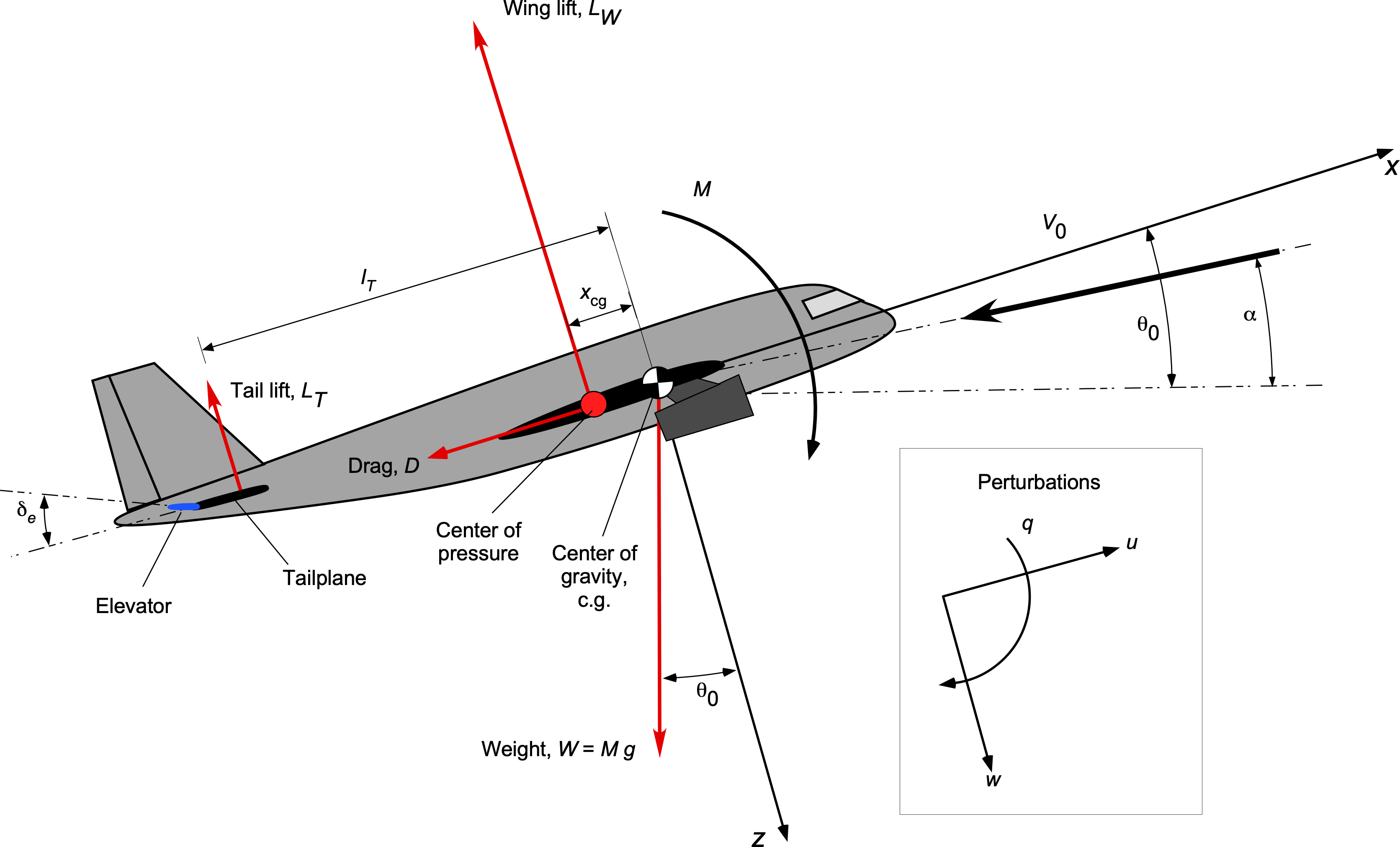
In reference to the figure, then the perturbation forces in the direction are
(20) 
For the perturbation forces in the direction, then
(21) 
Finally, for the perturbation in the pitching moment, then
(22) 
Longitudinal Static Stability
It is initially convenient to describe the principles concerning an airplane’s longitudinal or pitching response, mainly because the responses in pitch are clean and uncoupled from the responses in roll and yaw. Consider the situation when the balance of forces and moment in the trim state is disturbed, such as by a vertical gust caused by atmospheric turbulence. However, it should be remembered that gusts can come from virtually any direction, affecting the airplane’s response about any axis. Still, the vertical or velocity gusts typically have the most significant effects on the aircraft’s responses.
A vertically upward gust, , will cause an increase in the wing’s angle of attack, increasing its lift, and the airplane’s inherent reaction is that its nose will pitch up slightly. The consequence of this effect, is that the airplane is no longer in stable equilibrium and will deviate from its trimmed flight condition, as shown in the figure below. If the subsequent forces and moments generated on the airplane from the gust disturbance tend to return it to its trimmed condition, the airplane’s response would be referred to as being statically stable, as shown in scenario (b). Mathematically, when expressed in terms of a stability derivative, then
(23) 
which must be negative to produce a restoring moment.
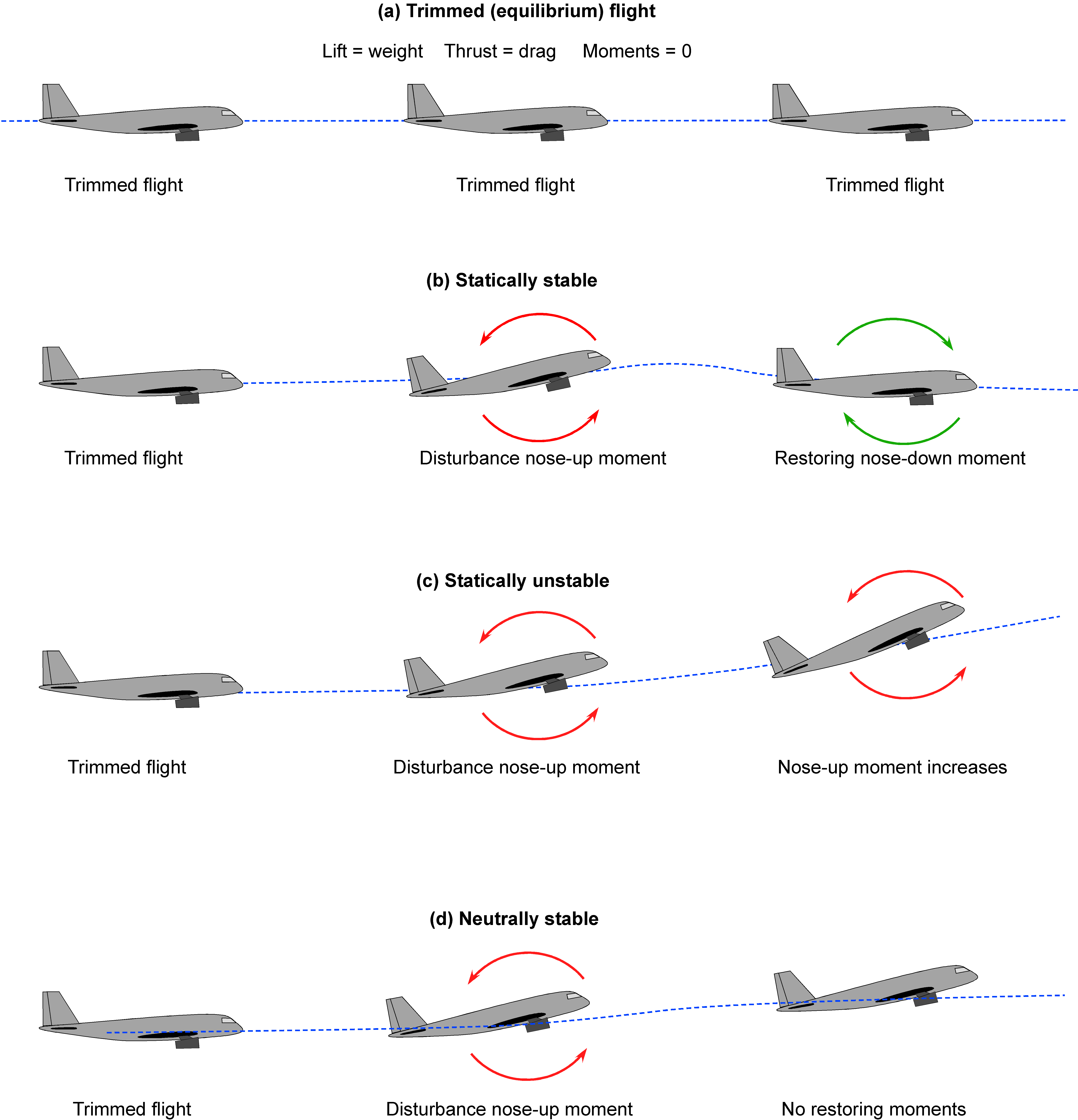
However, if the forces and moments introduced by the gust or other disturbance tend to cause the nose to pitch up further, then the airplane would be considered statically unstable, which is scenario (c). In this case,
(24) 
If the airplane is genuinely statically unstable, its subsequent motion may cause a divergence of the flight path and, most likely, a departure from controlled flight. When the airplane remains indefinitely disturbed, as shown in scenario (d), then it is considered to have neutral static stability, i.e.,
(25) 
but this is not a common characteristic of an airplane.
Static Margin
The conditions ensuring sufficient longitudinal static stability can now be formally established, leading to the parameter known as the static margin, which quantifies the static stability in pitch. The static margin is a distance measured in length units, although it is often expressed as a fraction or percentage of the mean wing chord.
Assuming the trim condition where  , for vertical equilibrium, then
(26) 
where is the weight of the aircraft,  is the wing lift, and
  is the tail lift. The wing lift is conventionally expressed as
(27) 
where  is the wing (reference) area,
  is the angle of attack, and
  is the zero-lift angle. Here,
  denotes the aerodynamic lift-curve slope of the wing (at the appropriate combination of Mach number and Reynolds number), which will either be assumed or determined from wind tunnel measurements.
The lift force from the tailplane also depends on its angle of attack (which will differ from that of the main wing) and is additionally affected by the upstream wing’s downwash, lowering its effective angle of attack by  . The resulting lift force on the tail may act upward or downward depending on flight conditions. Therefore, in trim
(28) 
where  is the horizontal tail area, is the elevator deflection angle, and
  is the lift-curve slope of the tail with respect to elevator deflection. Assuming the lift-curve slope of the tail to changes in and (but not ) is the same as that of the main wing, then
(29) 
In reference to the figure shown below, taking moments (positive nose-up) about the c.g. gives
(30) 
where  is the location of the c.g. relative to the aerodynamic center on the wing, and
  is the moment arm for the horizontal tail. In trim,
  . Differentiating Eq. 30 with respect to yields
(31) 
Considering the total lift as acting at a distance  behind the c.g., then
(32) 
Differentiating this equation with respect to gives
(33) 
For pitch stability,  must be negative for a positive change in . Therefore, both
  and
and  being positive implies must be negative, indicating the c.g. must be ahead of the c.p.
Assuming equal lift-curve slopes for the wing and tail, then
(34) 
(35) 
defines the static margin .
Assuming the flight controls (elevator in this case) are fixed and do not contribute to the aerodynamics ( ), termed “stick-fixed” response, in non-dimensional terms, then
(36) 
The mean chord  is the mean aerodynamic chord (MAC) of the main wing, i.e.,
(37) 
where  is the semi-span, and is the wing area. The parameter
(38) 
is called the non-dimensional tail volume coefficient for the horizontal tail (HT), typically ranging from  to
to  for conventional airplanes. For the vertical tail (VT), this coefficient, denoted by
  , is usually smaller, in the range from
  to
to  .
.
From Eq. 36, the location of the c.g. on the edge of static stability in pitch can be calculated, known as the neutral point  , i.e.,
(39) 
The neutral point serves as the pivot point of aerodynamic forces. Therefore, the static margin, defined as the distance between the neutral point (np or n.p.) and the c.g., is non-dimensionally expressed (based on preceding definitions and assumptions) as
(40) 
If the c.g. is ahead of the n.p., the aircraft is statically stable; if behind, it is unstable. For static stability, a negative static margin is required. However, the value is often quoted such that positive static stability corresponds to a positive static margin, i.e.,
(41) 
Check Your Understanding #1 – Estimating the static margin
Consider an airplane with a conventional tail. The airplane is trimmed for straight, level, and unaccelerated flight. The main wing has a lift curve slope of 0.08 per degree. The tail has a lift curve slope of 0.06 per degree and an estimated downwash of 0.1 deg per degree. The horizontal tail volume coefficient is 0.8. The center of gravity is at 0.36 aft of the datum. Estimate the static margin relative to the position of the center of gravity. Will the aircraft be statically stable?
Show solution/hide solution.
The static margin relative to the position of the center of gravity (c.g.) as a fraction of the mean chord can be expressed by
![\[ \dfrac{h_{~}}{\overline{\overline{c}}} = \dfrac{x_{cg}}{\overline{\overline{c}}} + \left( 1- \dfrac {\partial \epsilon}{\partial \alpha } \right) {\cal{V}}_{\rm HT} \]](https://eaglepubs.erau.edu/app/uploads/quicklatex/quicklatex.com-08e71b605cb128d1de5862f2f65d02eb_l3.svg "Rendered by QuickLaTeX.com")
However, in this case, with different lift curve slopes for the wing and the tail, the static margin must be written more generally as
![\[ \dfrac{h_{~}}{\overline{\overline{c}}} = \dfrac{x_{cg}}{\overline{\overline{c}}} + \left( 1- \dfrac {\partial \epsilon}{\partial \alpha } \right) \left( \dfrac{ \dfrac{\partial C_{L_{\rm HT}} }{\partial \alpha}}{\dfrac{\partial C_{L_{W}}}{\partial \alpha}} \right) {\cal{V}}_{\rm HT} \]](https://eaglepubs.erau.edu/app/uploads/quicklatex/quicklatex.com-db7afaaf2f89d31c0ef5733361599166_l3.svg "Rendered by QuickLaTeX.com")
The values of all the terms in the second term on the right-hand side of the equation are known. However, they must be converted into angular units of radians. For the downwash, then
![\[ \dfrac {\partial \epsilon}{\partial \alpha } = 0.1~\mbox{\small degrees per degree} = 0.1~\mbox{\small radians per radian} \]](https://eaglepubs.erau.edu/app/uploads/quicklatex/quicklatex.com-2e8634679cea52b34ff6a0c82f997bf4_l3.svg "Rendered by QuickLaTeX.com")
For the wing, then
![\[ \dfrac{\partial C_{L_{W}} }{\partial \alpha} = 0.08 \left( \frac{180}{\pi} \right) = 4.57~\mbox{\small per radian} \]](https://eaglepubs.erau.edu/app/uploads/quicklatex/quicklatex.com-a5b73d2101fdeaa0d4c95e197dd43a47_l3.svg "Rendered by QuickLaTeX.com")
For the horizontal tail, then
![\[ \dfrac{\partial C_{L_{\rm HT}} }{\partial \alpha} = 0.06 \left( \dfrac{180}{\pi} \right) = 3.44~\mbox{\small per radian} \]](https://eaglepubs.erau.edu/app/uploads/quicklatex/quicklatex.com-df1a13052f1f991623b0db5b83dfca94_l3.svg "Rendered by QuickLaTeX.com")
Therefore,
Entering the numerical values gives
![\[ \dfrac{h_{~}}{\overline{\overline{c}}} = \dfrac{x_{cg}}{\overline{\overline{c}}} + \left( 1- 0.1 \right) \left( \dfrac{3.44}{4.57} \right) 0.8 = -0.36 + 0.54 = 0.18 \]](https://eaglepubs.erau.edu/app/uploads/quicklatex/quicklatex.com-5139f880d21c4d3c73f0889723a4a0a2_l3.svg "Rendered by QuickLaTeX.com")
This result confirms that the aircraft has a positive static margin and is statically stable. Notice that the static margin is affected by the tail volume coefficient, so if that value becomes too small, the static margin can be reduced to unacceptable values, typically leading to adverse stability characteristics.
Sources of Longitudinal Stability
Notice from Eq. 36, that the horizontal tail significantly contributes to the static margin, with a more significant tail volume coefficient increasing the static margin. Indeed, a larger tail area will contribute more to the static stability, as well as a longer distance between the center of pressure on the tail and the wing.
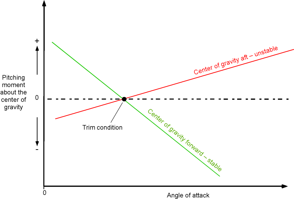
The typical steady (static) pitching moment contributions about the c.g. for a conventional airplane as a function of the angle of attack, are shown in the figure below. In this regard, a conventional airplane has a single wing and tail combination. There is a net-zero pitching moment at the trim angle of attack, . The sign convention is that positive moments are nose-up moments, i.e.,  , is positive nose-up, tending to increase the wing’s angle of attack and so having a destabilizing effect on the airplane. Notice that different pitching moment contributions (both in magnitude and sign) are caused by the various components of the airplane, e.g., the wing, the fuselage, and the tail, which all produce different aerodynamic effects. Therefore, these components produce other moments about the c.g.
The wing lift component by itself is destabilizing in that it produces a nose-up moment about the c.g., i.e., the slope of the moment curve, , is positive for the wing by itself. Likewise, the fuselage has a destabilizing effect. However, it can be seen that the horizontal tail produces a powerful nose-down moment about the c.g. with a negative slope of the moment curve, providing a significant stabilizing effect, hence the name “horizontal stabilizer” for the horizontal tail.
The combined effect of all the components on the entire airplane is a negative  slope, making the airplane statically stable. Generally, a larger horizontal tail will produce a more statically stable airplane, but the physical position of the tail on the fuselage relative to the c.g. (and other things) also plays an important role. In practice, the area of the tail surfaces must be enough to give the airplane sufficient pitch and directional stability. Still, too much stability will also make the airplane less maneuverable and often “tail-heavy” because of the larger sizes of the surfaces.
Therefore, one goal in airplane design is to give the tail surfaces sufficient area to obtain the needed stability characteristics but not too big so that they adversely affect weight and, e.g., location. It is common for tail surfaces to be undersized during the normal design process, which will become apparent after flight testing. Adding dorsal fins is often a solution, which can be done with minimal design changes, weight, and cost.
Check Your Understanding #2 – Horizontal and vertical tail sizing for static stability
In the preliminary design of a specific turboprop aircraft, it is required to estimate the size (areas) of the horizontal and vertical tails to give the aircraft sufficient longitudinal and yaw (directional) static stability. Using historical values of the tail volume coefficients for this class of aircraft,  = 0.80 and
  = 0.2, estimate the areas of both the horizontal and vertical tails if
  where the length of the fuselage,
  , is 46 ft. Assume that
  at the tail surfaces. The reference wing area,
  , is 300 ft2 with a mean chord, , of 5.2 ft.
Show solution/hide solution.
The horizontal tail volume coefficient can be expressed by
![\[ {\cal{V}}_{\rm HT} = \frac{l_{\rm HT} \, S_{\rm HT}}{\overline{\overline{c}} \, S_{W}} = \frac{0.53 \, l_F \, S_{\rm HT}}{\overline{\overline{c}} \, S_{W}} \]](https://eaglepubs.erau.edu/app/uploads/quicklatex/quicklatex.com-3bbb23ac9a0bd2a3f8ea9c33511ed193_l3.svg "Rendered by QuickLaTeX.com")
Therefore, the horizontal tail area needed for sufficient pitch stability will be
![\[ S_{\rm HT} = \frac{{\cal{V}}_{\rm HT} \, \overline{\overline{c}} \, S_{W}}{0.53 \, l_F} = \frac{0.8 \times 5.2 \times 300.0}{0.53 \times 46.0} = 51.2~\mbox{ft}^2 \]](https://eaglepubs.erau.edu/app/uploads/quicklatex/quicklatex.com-bc3e97e9a8c7d82c24fb54379c8fcb24_l3.svg "Rendered by QuickLaTeX.com")
Similarly, the vertical tail volume coefficient is given by
![\[ {\cal{V}}_{\rm VT} = \frac{l_{\rm VT} \, S_{\rm VT}}{\overline{\overline{c}} \, S_{W}} = \frac{0.53 \, l_F \, S_{\rm VT}}{\overline{\overline{c}} \, S_{W}} \]](https://eaglepubs.erau.edu/app/uploads/quicklatex/quicklatex.com-091d640fb24961bc82350f6dc04de9c8_l3.svg "Rendered by QuickLaTeX.com")
Therefore, the vertical tail area needed for sufficient directional (yaw) stability will be
![\[ S_{\rm VT} = \frac{{\cal{V}}_{\rm VT} \, \overline{\overline{c}} \, S_{W}}{0.53 \, l_F} = \frac{0.8 \times 5.2 \times 300.0}{0.53 \times 46.0} = 12.8~\mbox{ft}^2 \]](https://eaglepubs.erau.edu/app/uploads/quicklatex/quicklatex.com-7e0a9eecda899506de0b4f05af8a16c5_l3.svg "Rendered by QuickLaTeX.com")
Dynamic Stability
If the airplane is statically stable in pitch, then the restoring forces and moments acting upon it will cause the nose of the airplane to pitch down again after the initial disturbance. The same is true for yaw and roll disturbances in that yaw and roll will cause a return to the trim state if the aircraft has positive static stability. However, this desirable static response does not necessarily mean the airplane will immediately settle and reestablish its original trimmed state. So, the question becomes: What happens to the airplane response(s) in subsequent time, i.e., the dynamic response?
To this end, several possibilities could happen:
1. The airplane may continue to pitch nose-down and overshoot the initial trimmed state. Then the nose comes back up and returns toward trim but overshoots again. This process may continue in a series of nose-up and nose-down pitching motions, i.e., an oscillating or oscillatory response. Suppose these oscillatory motions eventually damp out over time and cause the airplane to return to the initial trim. Then, this decaying oscillatory motion means that the airplane is dynamically stable.
2. The airplane does not overshoot the trimmed state and settles out quickly to reestablish its trim, which is called subsidence. In this case, the airplane is dynamically stable, and the damping is said to be critically damped or to have a “deadbeat” response. Some airplanes exhibit this characteristic, but most do not because they would have to have larger than desirable horizontal tail surfaces, which, from a structural design perspective, becomes a weight issue.
3. The airplane may continue with a continuous nose-up and down pitching motion, with the subsequent oscillations in pitch remaining at an almost constant amplitude. In this case, the airplane’s resulting “roller-coaster” dynamic response exhibits neutral dynamic stability. While the pilot can dampen long-period responses by applying compensatory flight control inputs, it is still an undesirable response for an airplane.
4. In a worst-case scenario, the airplane may respond with nose-up and nose-down pitching oscillations with increasing amplitude. This type of response would be called a dynamically unstable response. As with weak or neutral damping, an unstable aircraft does not necessarily mean it is unsafe if the unstable tendency has a long period (10s of seconds) and can be controlled by the pilot.
Notice that an airplane must be statically stable to be dynamically stable, i.e., a prerequisite for dynamic stability is static stability. Therefore, a statically unstable airplane will also be dynamically unstable. A statically and dynamically stable airplane is generally easier to fly and control. However, an airplane may be statically stable and dynamically unstable but still perfectly flyable, especially if the dynamic response is slow enough for the pilot to control it by employing appropriate “damping” flight control inputs. Short period response are very difficult for the pilot to control.However, such an aircraft generally has inferior flying qualities and can impose a high workload on the pilot. The dynamic response may also depend on the aircraft’s weight, the c.g. location, and airspeed.
Longitudinal (Pitch) Stability
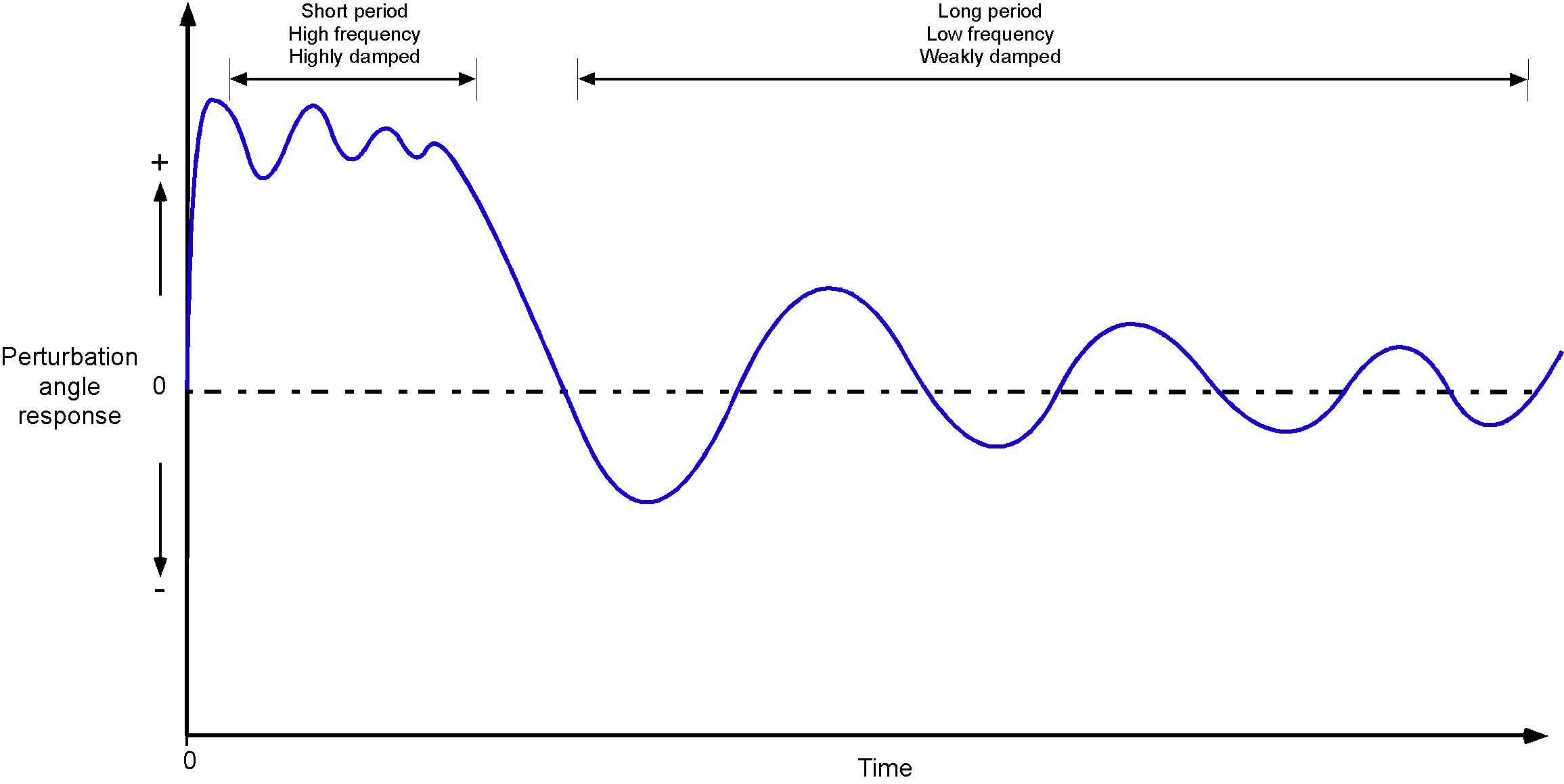
Dynamic pitch stability refers to the behavior of an aircraft’s pitch angle (the angle between its longitudinal axis and the horizon) over time after it has been disturbed from its equilibrium state. Two forms of longitudinal dynamic and oscillatory responses are found with airplanes: The long period dynamic response and the short-period dynamic response, as shown in the figure below for the pitch motion. On the one hand, the short-period response is typically highly damped and lasts less than a second. On the other hand, the long-period or phugoid mode of oscillation is a slower, weakly damped oscillation of the aircraft’s flight path over many seconds or even minutes.
Short-Period Response
As shown in the figure below, the short-period oscillatory response mode is of a higher frequency and is a highly damped oscillatory response, often appearing in the airplane’s dynamic response after encountering gusty air or applying quick elevator inputs, such as during landing. However, the short-period response is usually unnoticed by the pilot and does not have to be controlled. All three flight axes will typically show short-period dynamic responses, which in all cases will quickly be damped out.
However, in some circumstances, the pilot may inadvertently excite the short-period responses, such as during landing or in severe turbulence when quick, deliberate movements of the control stick are being made to adjust the aircraft’s flight attitude. In particular, a landing requires significantly increased attention from the pilot on the controls. In some cases, the pilot’s control inputs may become entirely out of phase with the aircraft’s short-period response, resulting in what is known as a pilot-induced oscillation (PIO).
A PIO is just one type of Aircraft-Pilot Coupling (APC) effect. A PIO is often a hazardous flight condition because the pilot’s inputs may cause the short-period response to become quickly divergent, resulting in a mishap or a crash. Most pilots initially tend to induce APC effects when flying sailplanes or jet fighters, which have relatively sensitive flight controls. The solution to the development of a PIO is for the pilot to relax their grip on the flight controls, which takes that pilot’s out-of-phase inputs out of the control loop, allowing the response to damp out.
Long-Period Response
The term “phugoid” was initially coined by Frederick Lanchester for the dynamic pitch response of an aircraft; the word has a literal translation from Greek meaning “fleeing,” so it is a misnomer. The figure above shows that the phugoid response is typically a weakly damped dynamic response. Still, it is easily damped out by pilot control inputs using the elevator and so is easily controlled by the pilot, even if the response is weakly divergent. The phugoid frequency,  , depends on the airspeed of the airplane,
  , where
  is the initial trimmed airspeed, according to
(42) 
which is a result for small perturbations.[2] The damping in the pitch mode depends on the aircraft’s lift-to-drag ratio, as given by
(43) 
Therefore, the phugoid response tends to be very pronounced and weakly damped on airplanes with high lift-to-drag ratios, e.g., sailplanes. Still, the pilot can easily control the airplane with corrective elevator inputs because the response occurs over long periods.
Analysing the Long-Period Response
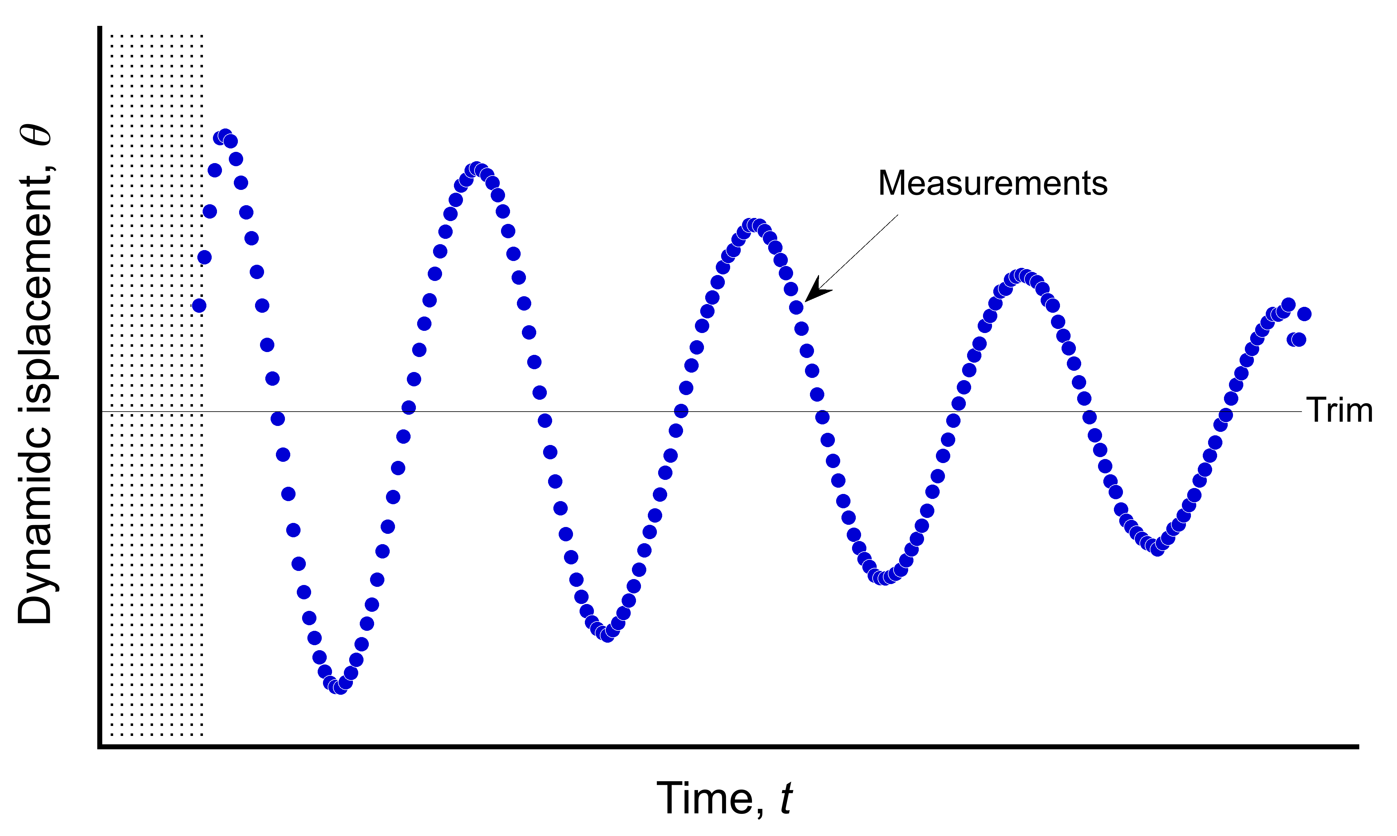
The long-period response is one of the most interesting aspects of the flight dynamic behavior of any aircraft, which is typically a weakly damped oscillatory motion. Representative in-flight measurements are shown in the figure below, although such results could also come from a flight dynamic simulation using solutions from the equations of motion. These types of responses are obtained by disturbing the aircraft about its trimmed condition by the sudden (abrupt) application of flight controls and then measuring the displacements using suitable instrumentation, such as angle of attack sensors and accelerometers. If sufficiently large, the resulting angle of attack excursions can often resemble a roller-coaster ride!
Characteristic Response
For disturbances about a mean or trim angle, the dynamic motion can be described using the equation
(44) 
where is the angular displacement,  is the trim angle,
  is the undamped natural frequency of the dynamic motion, and
  is the damped frequency of the motion. The constants
  and are constants that can be determined from the conditions at the application of the initial disturbance, which are arbitrary.
The damped natural frequency is related to the undamped frequency using
(45) 
where  is the damping coefficient. Notice that the damped frequency is always less than the undamped frequency. The parameter of primary interest from flight-test measurements is the damping of the dynamic response, which can be expressed as a logarithmic decrement.
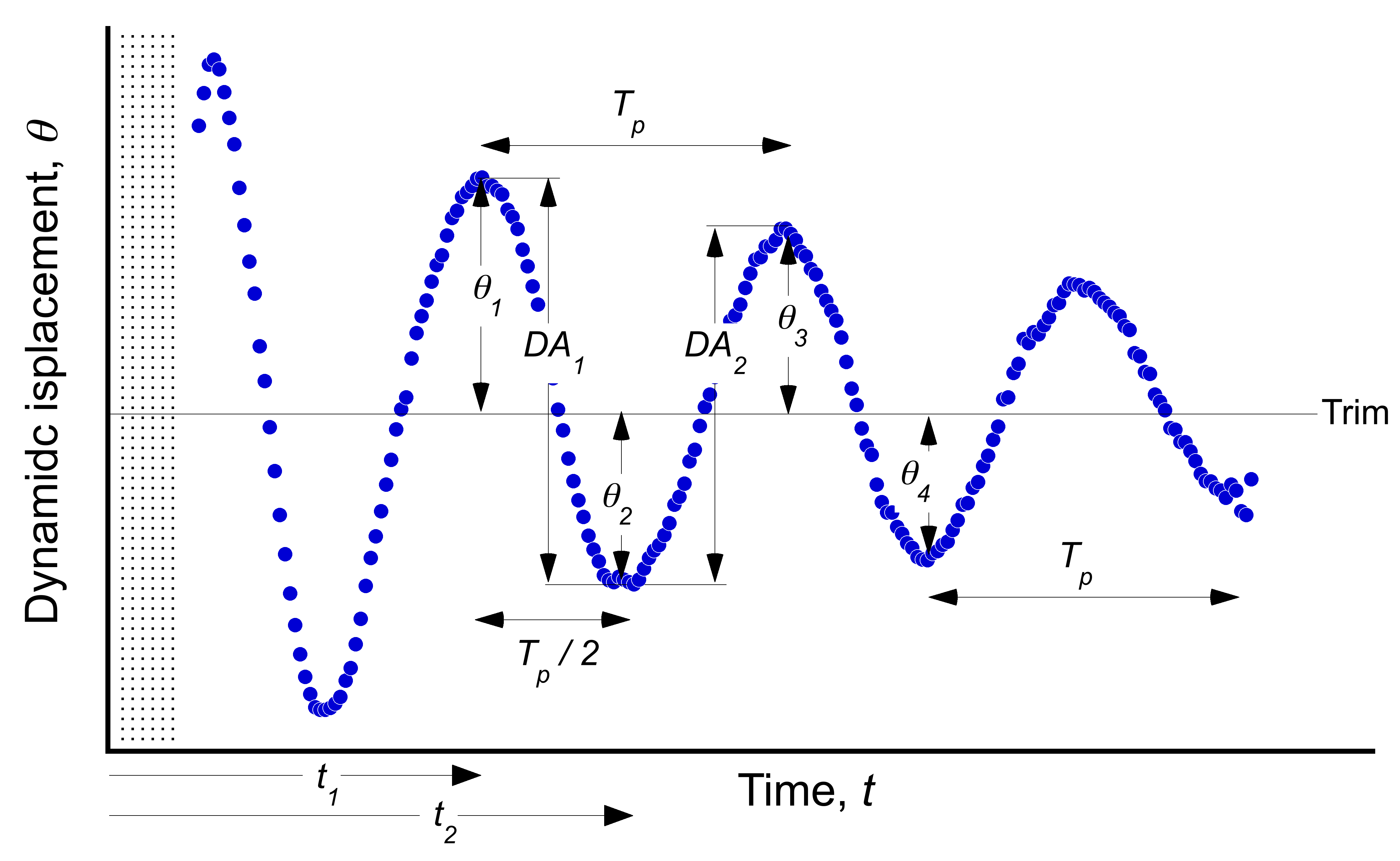
The logarithmic decrement represents the rate at which the amplitude of the phugoid displacement decreases. It can be defined as the ratio of any two of the successive amplitudes in the time history of the motion. These amplitudes could be peaks or valleys in the motion, so different methods of estimating the damping can be devised. In the ideal cases, measurements of the complete time history of the aircraft’s dynamic motion will be available. In other cases, only the times of the peaks and valleys in the dynamic response may be available for analysis. If any of these results are available, the damping of the dynamic motion can be estimated.
Method of Analysis
Let  and
and  be the times corresponding to a successive peak and valley or a successive valley and a peak in the dynamic response. These displacements should be measured about the trim angle and half a cycle apart, i.e.,
  , as shown in the figure below.
The displacements at these two times are
(46) 
and
(47) 
Therefore, the ratio of the displacements is
(48) 
Because the two peaks are defined to be exactly one cycle apart, then
(49) 
where  is the period of the dynamic response. Therefore,
(50) 
Using this result, the ratio of the peaks can now be written as
(51) 
To improve the accuracy of the estimated damping, an average can be obtained of the ratios formed at successive peaks in the motion. This average is called the Transient Peak Ratio or TPR method. The value of the TPR can be written as
(52) 
where is the number of ratios formed, i.e.,
(53) 
Therefore, using Eq. (8), the logarithmic decrement can be written as
(54) 
The damped and undamped natural frequencies are related using  , so can be written as
(55) 
Rearranging this equation gives the average damping, , as
(56) 
where  . Therefore, with knowledge of the value of the TPR, the damping, , can be determined.
To find the value of the TPR, let the net amplitudes of successive peaks and valleys or valleys and peaks be  ,
,  ,
,  , etc. For example, taking the
  term gives
(57) 
Because and are exactly one-half cycle apart, then
(58) 
where is the cycle time or period of the dynamic response. Therefore,
(59) 
and is given by
(60) ![\begin{eqnarray*} DA_1 & = & A e^{-\zeta \, \omega_n \, t_1} \sin( \omega_d \, t_1 + \phi ) + A e^{-\zeta \, \omega_n (t_1 + T_p/2)} \sin( \omega_d \, t_1 + \phi ) \\[12pt] & = & A e^{-\zeta \, \omega_n \, t_1} \sin( \omega_d \, t_1 + \phi ) \left[ 1 + e^{-\zeta \, \omega_n \, T_p/2} \right] \end{eqnarray*}](https://eaglepubs.erau.edu/app/uploads/quicklatex/quicklatex.com-b10866325662f850a3d07cdfa089158a_l3.svg "Rendered by QuickLaTeX.com")
Similarly,  is given by
(61) ![\begin{equation*} DA_2 = A e^{-\zeta \, \omega_n \, t_2} \sin( \omega_d \, t_2 + \phi ) \left[ 1 + e^{-\zeta \, \omega_n \, T_p/2} \right] \end{equation*}](https://eaglepubs.erau.edu/app/uploads/quicklatex/quicklatex.com-53dda377ed8610a8ef0a2771e9618cbd_l3.svg "Rendered by QuickLaTeX.com")
The ratio of successive  displacements will be
(62) 
Using the result that  , the ratio of the displacements can be written as
(63) 
Therefore, the  can be written as
(64) 
where is the number of ratios formed, i.e.,
(65) 
The value of is given by
(66) 
and so the damping, , by
(67) 
where .
An average of the period for one cycle of the long-period dynamic response can be found using
(68) 
and the average value of the damped frequency is found from
(69) 
Finally, the undamped frequency of the dynamic motion can be found using
(70) 
Center of Gravity Effects & Limits
As previously discussed, the c.g. location of an airplane is critical because it has a powerful effect on its stability and control characteristics, e.g., if the c.g. moves with respect to the neutral point or if the neutral point moves (because of compressibility effects) with respect to the c.g. If the c.g. location moves progressively aft (toward the tail), such as when fuel is burned off, then the moment curve slope becomes less negative, and will eventually become zero at the neutral point; in this case, the airplane will have neutral static stability.
If the c.g. is moved further back, the airplane will become unstable. This behavior can become a problem on some airplanes if the c.g. moves too far rearward, such as when a load is discharged in flight, e.g., weapons, cargo, parachutists, etc. Likewise, for whatever reason, suppose the c.g. moves toward the nose. In that case, the moments must be trimmed out using elevator control inputs or a horizontal tail with trim capability. Eventually, suppose the c.g. location moves too far forward so that the upward elevator displacements on the tail surfaces will not generate enough aerodynamic force to be enough to compensate. In this case, the airplane cannot be trimmed and will become unflyable, nosing down toward the ground and building up airspeed, often with a catastrophic outcome.
It is clear, therefore, that design engineers must carefully establish the c.g. limits (fore and aft) on all airplanes to ensure that they fall within an acceptable range for safe flight and that any c.g. movements during the flight will not compromise their stability and control characteristics. An example of a c.g. chart for an airplane is shown in the chart below. Based on the estimated takeoff weight and the calculated c.g. location, the values must lie within the aircraft’s defined and certified envelope to be safe to fly.
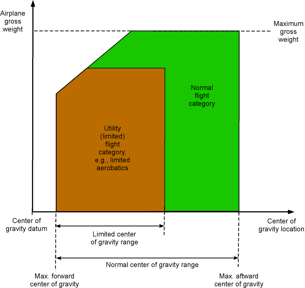
In practice, the pilot must be sure that the airplane is loaded correctly before the flight with all passengers and cargo, etc., takes off and that the c.g. location is within limits. Indeed, airplanes have crashed because they were not loaded correctly, the cargo moved during flight, or fuel and weight were burned off moving the c.g., and the airplane either became unstable or the control forces became too high for the pilot to control the aircraft.
Lateral (Roll) Stability
Lateral stability and control refer to displacements about the longitudinal or roll axes. For example, an airplane has lateral static stability if, after a disturbance is applied, it rolls and acquires a bank angle but simultaneously generates new aerodynamic forces and moments that tend to reduce the bank angle and bring the airplane back to the initially trimmed flight condition. All airplanes have at least some inherent lateral stability, although because roll and yaw responses are coupled, the resulting dynamic response characteristics tend to be more complicated.
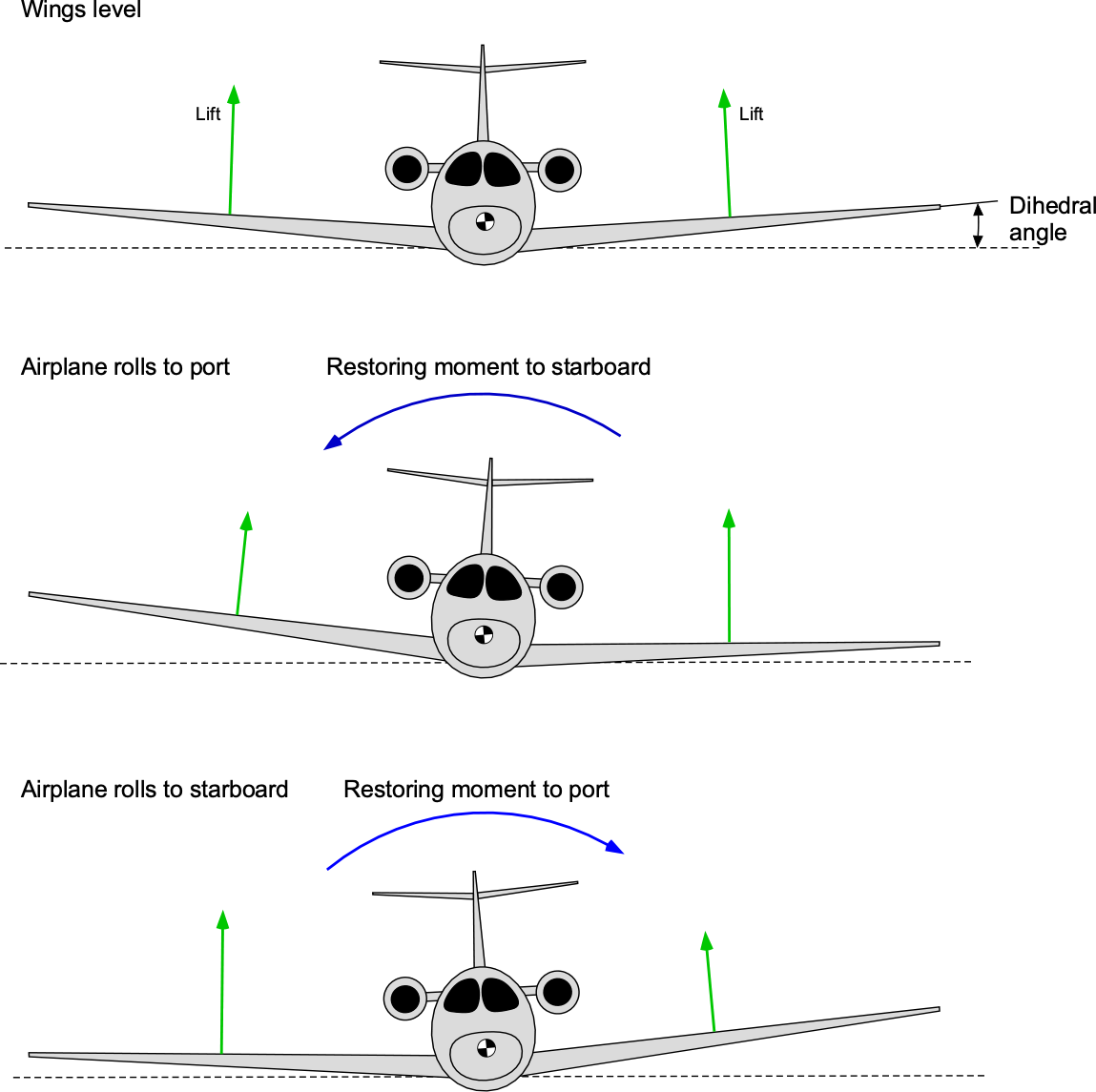
It is well known that using dihedral on the wings is a powerful means of providing an airplane with increased static lateral stability, as shown in the figure below. Just a few degrees of dihedral can make marked improvements to lateral stability. The horizontal tail may also have some dihedral, contributing somewhat to the lateral stability, as shown in the figure below.
The rolling moment coefficient, , can be expressed as a function of the roll angle , roll rate , sideslip angle , and other contributing factors as
(71) 
For an aircraft to be stable in roll, any roll disturbance should result in a restoring rolling moment, , as determined by the coefficient  , i.e.,
(72) 
where  is the span of the wing and is the wing (reference) area. Notice that wing span is being used as the reference length rather than the mean chord. Mathematically, roll motion can be expressed as
(73) 
So, for roll stability
(74) 
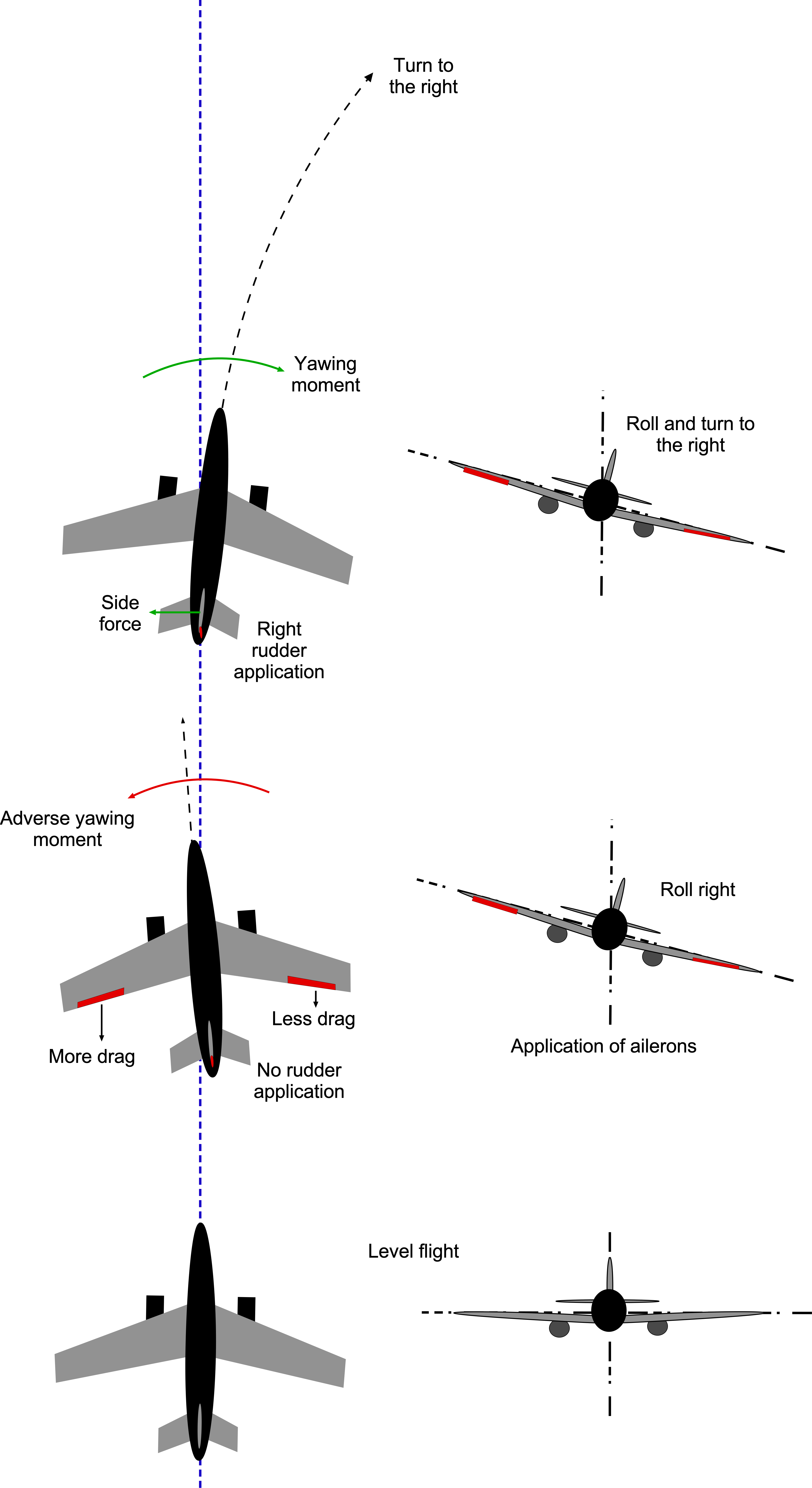
Using dihedral, however, tends to enhance the coupling between yaw and roll control inputs, i.e., rudder and aileron, respectively, so when the airplane yaws in one direction and develops a sideslip angle, it also tends to roll in that same direction. The pilot’s application of ailerons to produce a roll response and initiate the turn is also accompanied by different changes in lift and drag on each wing (port and starboard). The consequence is to cause a yaw response in the opposite direction to the turn, as shown in the figure below. The resulting behavior is called adverse yaw, and is particularly pronounced on airplanes with longer wing spans. The piloting solution is first to slightly lead the turn using the rudder to compensate for any adverse yaw response when the ailerons are applied. With its long, slender wings, a sailplane has powerful adverse yaw effects and must be flown with constant use of rudder inputs to lead the roll (aileron) inputs to prevent adverse yaw.
The vertical position of the wing relative to the c.g. of the aircraft also affects lateral stability, i.e., airplanes with a high-mounted wing versus a low wing. A high-wing airplane design naturally tends to have better lateral stability than a low-mounted wing because the c.g. is below the wing’s center of pressure, giving a form of pendular stability. This behavior is why dihedral is not a common design feature on high-wing airplanes. Some airplanes with high-mounted wings may use wings with only partial dihedral, such as on the outer wing panels, but this feature is rare.
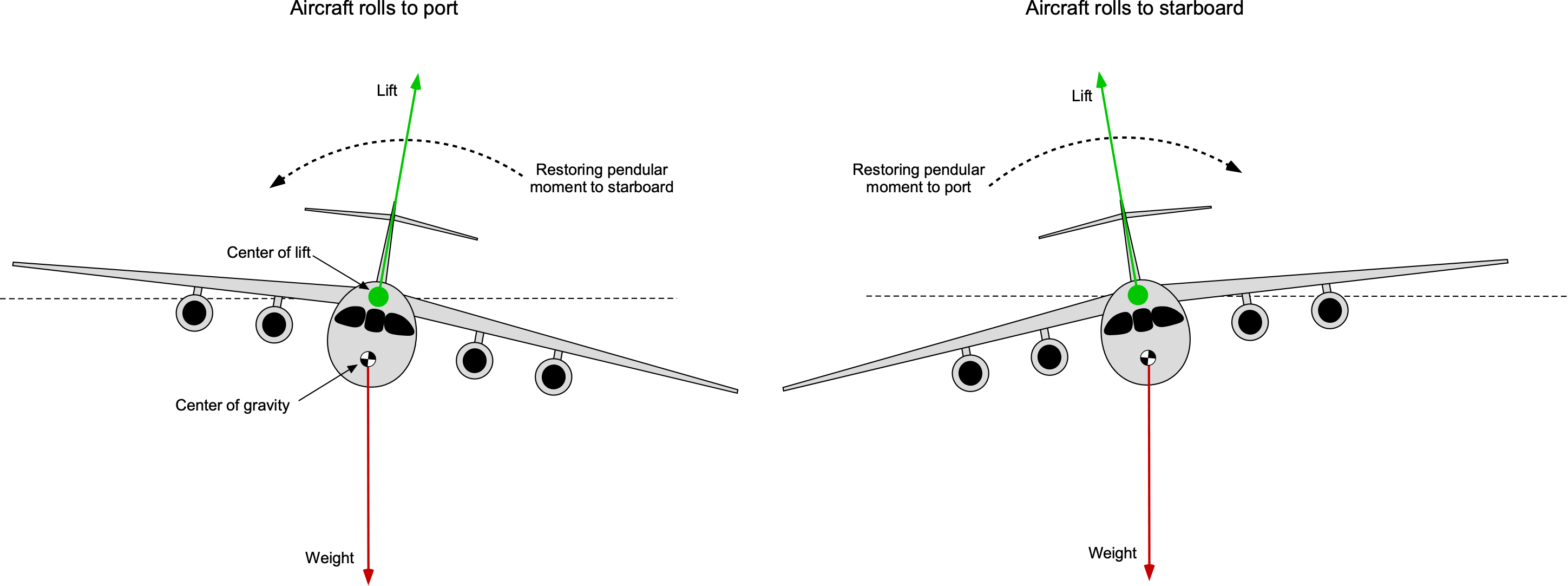
Wing sweep is used on high-speed airplanes to reduce compressibility drag, but wing sweep gives significant increases in lateral stability. A combination of wing dihedral and wing sweep often gives an airplane too much lateral stability. Therefore, airplanes with highly swept wings may use anhedral to negate the inherent lateral stability caused by wing sweep. Furthermore, on a large/heavy airplane with a high-mounted wing configuration, e.g., the C-5 Galaxy, there is usually excess pendular roll stability because the c.g. lies below the center of the lift, as shown in the figure below. The center of lift can be assumed to be the aerodynamic “pivot” point. In this case, anhedral on the wing is needed so that the lateral stability is not too strong to make the aircraft difficult to turn and maneuver.
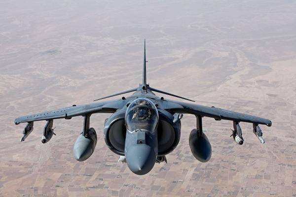
Anhedral on a fighter aircraft is needed to maintain its agility and maneuverability, as shown in the photo below. Fuselage and vertical tail effects may contribute to or detract from the airplane’s lateral stability, but this depends on the shape of the fuselage and the side of the vertical tail.
Directional Stability
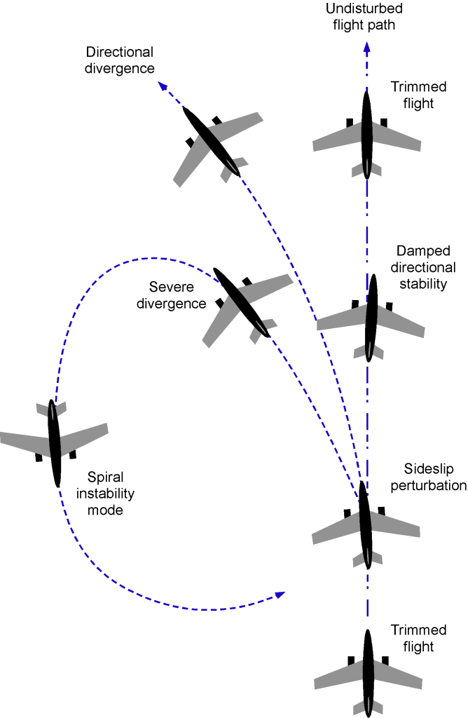
Dynamic flight responses are also associated with an airplane’s directional (yaw) or weathercock motion. However, as already mentioned, an airplane’s static lateral (roll) and directional (yaw) stability characteristics are intrinsically coupled, i.e., a roll response causes a yaw response and vice-versa. This coupling also affects the dynamic response, i.e., what happens to the airplane at longer times after a disturbance in roll or yaw. This so-called cross-coupling between the directional and lateral static stability can give rise to three important dynamic responses: a directional divergence mode, spiral divergence mode, and the “Dutch roll” mode.
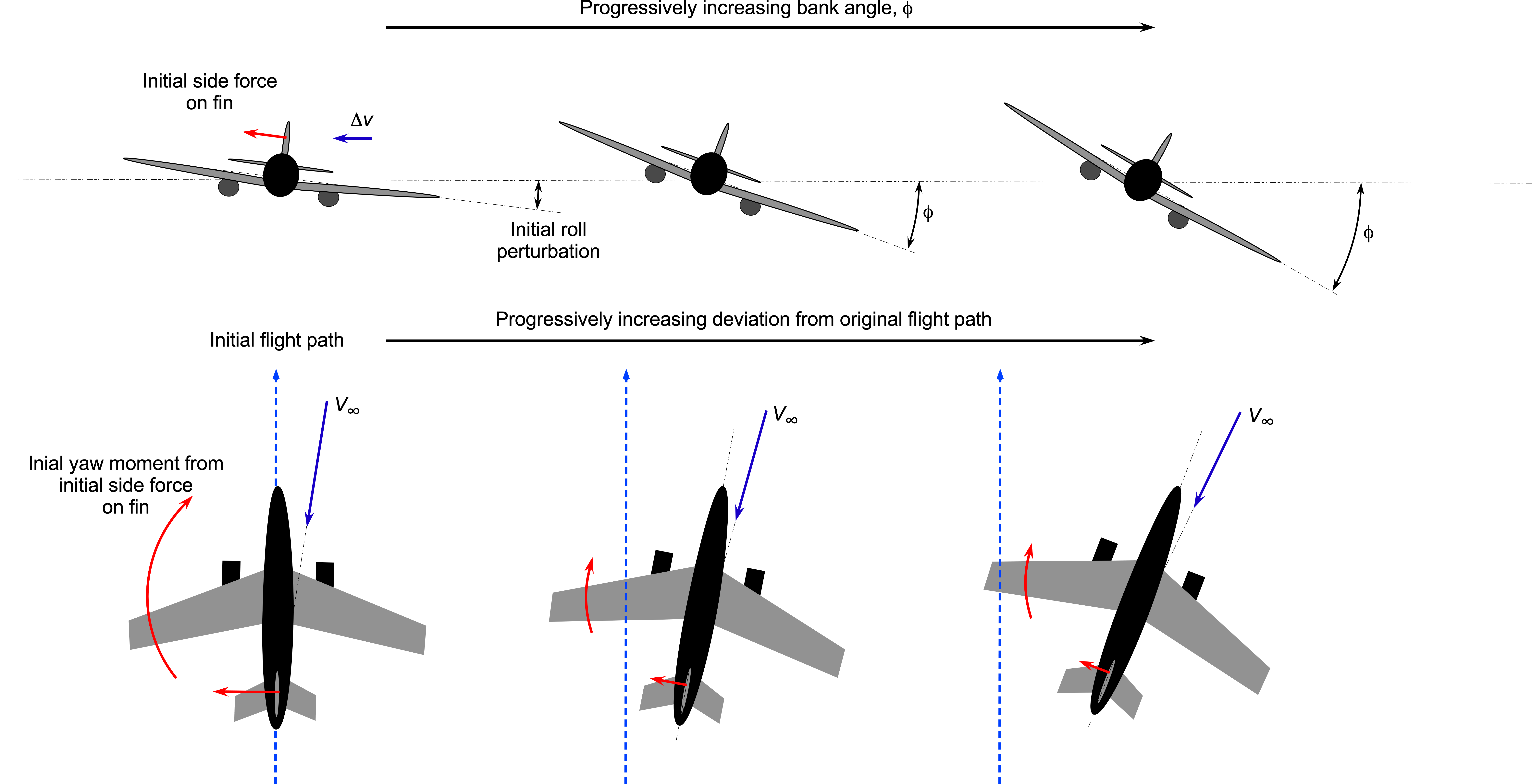
Directional Divergence
The directional divergent response results from a directionally unstable airplane, as explained in the figure below. When the airplane yaws or rolls into a sideslip, side forces on the airplane are generated, and the yawing moments that arise can continue to increase the sideslip and result in significant yaw angles. Recovery is accomplished by the normal use of flight controls. However, the concern is that the vertical tail can stall for steep angles, reducing its aerodynamic effectiveness to pilot rudder inputs and making recovery difficult. For this reason, not only is the sizing of the vertical tail essential to give sufficient directional stability, i.e., in providing adequate surface area, but also in controlling its higher yaw angle of attack behavior.
Quantifying the directional divergence requires the evaluation of the stability derivatives with respect to yaw, particularly the yawing moment coefficient derivative with respect to sideslip angle,  . The yawing moment coefficient can be expressed as a function of the sideslip angle, , yaw rate, , and possibly other contributing factors, as
(75) 
where  is the yawing moment coefficient at zero sideslip, is the yawing moment coefficient derivative with respect to sideslip angle, and
  is the yawing moment coefficient derivative with respect to yaw rate.
A disturbance in yaw should result in a restoring yawing moment for an aircraft to be considered directionally stable, which is indicated by a negative value of . Mathematically, this condition can be stated as
(76) 
For directional stability, then
(77) 
However, if
(78) 
then the airplane will be directionally divergent, which is an undesirable flight characteristic.
Spiral Divergence
Spiral divergence occurs if the coupling between roll and yaw leads to an unstable spiral motion. The spiral divergence mode tends to be pronounced on an airplane that is very stable directionally (about the axis yaw) but is not as stable laterally. This behavior relates to the size of the vertical fin versus the amount of dihedral on the main wing. The tendency to exhibit spiral divergence is reduced by increasing the dihedral on the wing. When the airplane is in a bank, the aerodynamic forces tend to turn the plane more deeply into the bank, and the nose drops, resulting in an ever-tightening downward spiral with increasing airspeed, as shown in the figure below.
This instability can be analyzed by examining the specific stability derivatives  ,
,  ,
,  , ,
, ,  , and . Generally, for spiral stability to develop, then must be positive and large, and the lateral stability or dihedral effect, , must be small or negative. The interaction of these stability derivatives can lead to a situation where an initial roll disturbance causes a yaw response that will further increase the roll angle, resulting in an ever-tightening spiral. The condition for spiral divergence to occur is
(79) 
Most airplanes exhibit a spiral instability mode, but it is usually very slow to develop, and the airplane can be quickly recovered to a level flight attitude through appropriate flight control inputs, i.e., bringing the wings level using ailerons and the elevator to regain a level pitch attitude. Of course, this assumes that the pilot has visual references to the horizon and the ground or the equivalent in terms of instrument readings. Unfortunately, suppose a spiral divergence occurs in the clouds without a clear reference to the horizon, and the pilot cannot interpret (or believe) the instruments correctly. In that case, the divergence can continue with increasing airspeed and bank angle into what pilots know as a “Graveyard spiral.”
A contributing human factor in the case of a graveyard spiral is the possibility of spatial disorientation resulting from the vestibular response in the pilot’s ears (which tell the brain about balance and orientation) that the forces on the aircraft are in equilibrium even though airspeed and bank angle are increasing. Corrective control inputs, in this case, by pulling back on the controls to decrease airspeed, serve only to tighten the radius of the spiral and increase the rate of descent. If this characteristic is allowed to continue, then the aircraft will eventually crash into the ground.
Dutch Roll
The “Dutch roll“[3] response of an airplane is a weaving dynamic response mode coupled with both the directional and spiral divergence modes. For most airplanes, the lateral stability is always fairly good, whereas the directional stability can be weaker. This behavior is especially so if the tail is even slightly undersized during design, which tends to be a relatively standard approach to save airframe weight; airplane designs generally always become tail-heavy if stability requirements are to be completely satisfied.
If a sideslip disturbance occurs, the airplane yaws in one direction, and the airplane rolls the other away in the form of a weaving motion, as illustrated in the figure below. While this motion is relatively low-frequency and usually well-damped, it is incredibly annoying during flight for the crew and passengers, if not uncomfortable. In addition, on some airplanes, the Dutch roll mode can become weakly divergent, which is always cause for concern. In this case, a yaw damper, which is part of the flight control system (autopilot), is used to damp out the Dutch roll mode and improve the flying qualities; the damper is switched on soon after takeoff and switched off again just before landing. Most jet aircraft with swept wings require a yaw damper to prevent an excessive Dutch roll response.
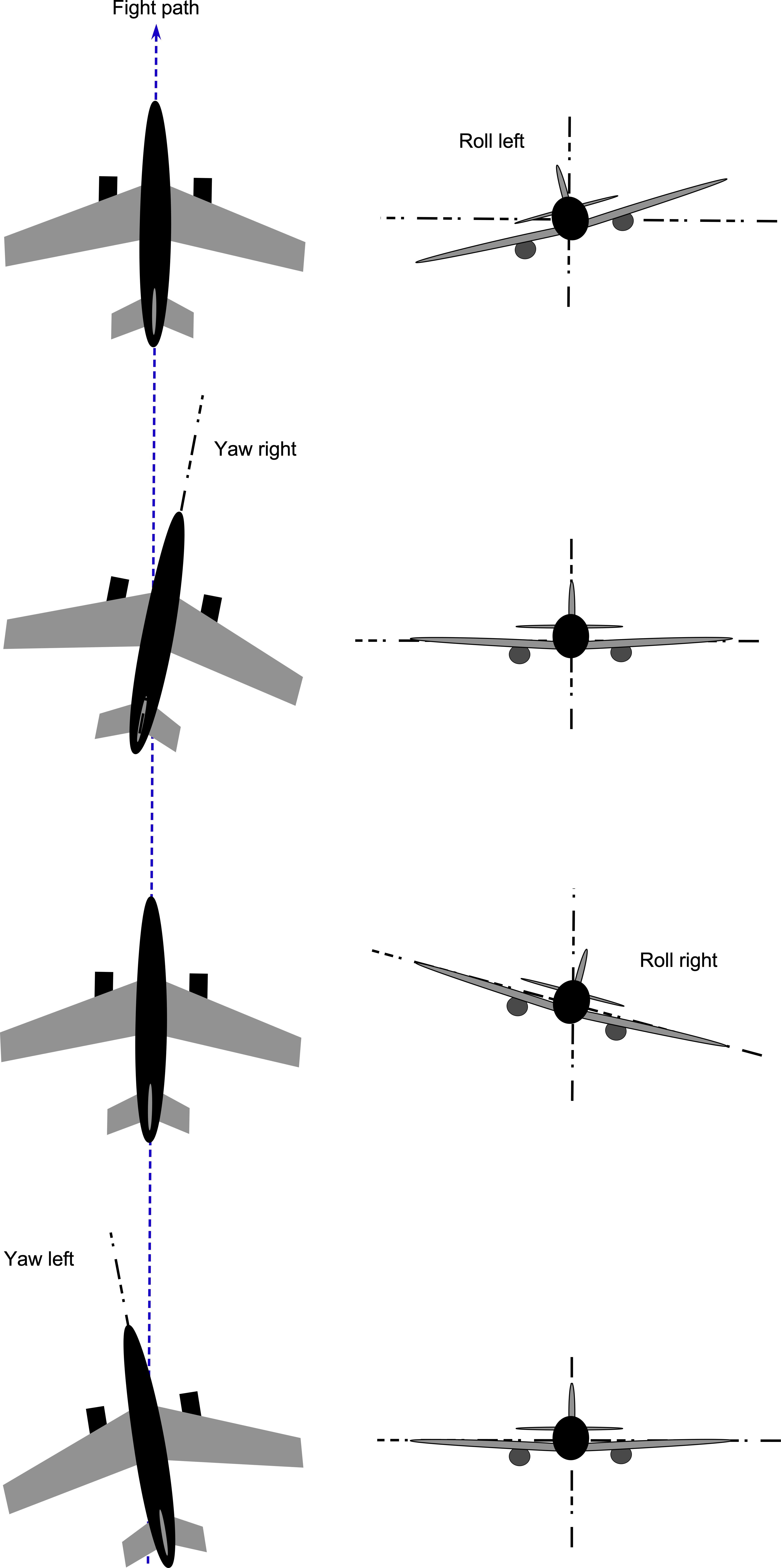
Analysis of the Dutch Roll Response
The Dutch roll motion can be described using linearized equations of motion for small perturbations around a steady flight condition. For the yaw or sideslip angle, the equation of motion is
(80) 
where is the sideslip angle, is the yaw rate,  is the moment of inertia around the -axis, and
  and
and  are the corresponding stability derivatives. The corresponding equation of motion for roll is
(81) 
where  is the moment of inertia around the -axis,
  and
and  are stability derivatives related to roll. Combining these equations into differential equation (state-space) form, let
  be the state vector, so that
(82) ![\begin{equation*} \begin{bmatrix} \dot{\beta} \\[22pt] \dot{r} \\[22pt] \dot{p} \end{bmatrix} = \begin{bmatrix} \dfrac{N_{\beta}}{I_z} & \dfrac{N_r}{I_z} & 0 \\[10pt] 0 & -\dfrac{1}{\tau_r} & \dfrac{\tau_{rp}}{\tau_r} \\[10pt] \dfrac{L_{\phi}}{I_x} & \dfrac{L_r}{I_x} & -\dfrac{1}{\tau_p} \end{bmatrix} \begin{bmatrix} \beta \\[22pt] r \\[22pt] p \end{bmatrix} \end{equation*}](https://eaglepubs.erau.edu/app/uploads/quicklatex/quicklatex.com-5efd4dc8e59a92820ad5491ee73e18f8_l3.svg "Rendered by QuickLaTeX.com")
where  and
and  are time constants for the yaw and roll rates, respectively, and
  is a coupling term between yaw and roll rates.
The time constants (yaw rate) and (roll rate) are crucial in aircraft dynamics as they describe how quickly the aircraft responds to perturbations in yaw and roll, respectively. A smaller value of indicates faster damping of yaw oscillations, improving directional stability and making the aircraft more responsive to rudder inputs. Similarly, a smaller means quicker damping of any roll oscillations, thereby improving lateral stability and responsiveness to aileron inputs. Both time constants are critical in ensuring the aircraft quickly stabilizes after disturbances, contributing to smoother flight.
These time constants are particularly significant in the context of the Dutch roll, which involves the coupled yaw and roll movements. Proper determination and eventual tuning of the values of and helps achieve balanced damping of these oscillations, preventing sustained oscillations that could affect the flight dynamics and control. Additionally, the coupling term describes the interaction between yaw and roll rates, which is critical to developing Dutch roll oscillations. These parameters can be adjusted through airframe design to ensure desirable handling qualities and stability. In most cases, stability augmentation systems, such as yaw dampers, may be used to improve flight characteristics.
Design Factors Influencing Dutch Roll
The vertical tail provides most of an airplane’s static directional stability, significantly affecting the Dutch roll response. An airplane is said to possess lateral directional or yaw stability if the aircraft yaws after a disturbance is applied but simultaneously generates new aerodynamic forces and moments that tend to dampen out the yaw displacement. However, the combined size and depth of the fuselage and the vertical tail’s height, area, and shape, ultimately affect an airplane’s directional stability characteristics.
For example, suppose an airplane experiences a sideslip angle. In this case, the fuselage produces a side force that tends to increase that angle, similar to what the fuselage does for the pitch response. Deep fuselages with boxy or deep elliptical cross-sections tend to be much worse in terms of directional stability than fuselages with circular cross-sections. During the design process, such issues are often explored by wind tunnel testing. A design goal is to shape the fuselage to minimize the static instability and so minimize the size of the tail, hence saving on airframe weight.
Fuselages with more area forward of the airplane’s c.g., tend to have less directional stability. Examples are the Boeing 747 and the C-5 Galaxy, which have large vertical tails to compensate for the large “hump” on the forward fuselages. The Airbus A380 had similar design issues, so it has a large vertical tail. The somewhat “disproportionately” large vertical fin and horizontal tail sizes of the A380 or the shorter fuselage on the Boeing 747SP (Special Performance) are also distinctive, as shown in the photograph below, which is needed to give sufficient static and dynamic stability and to minimize Dutch roll.
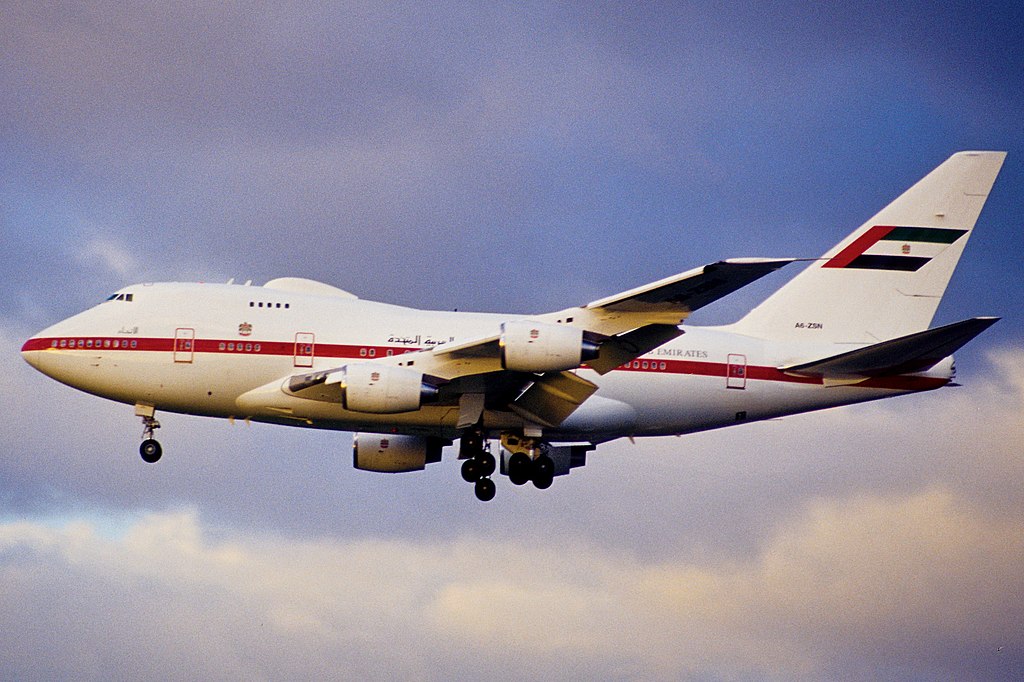
Ventral and/or dorsal fins are used on some airplanes to augment the directional stability and/or reduce the tendency to develop a Dutch roll, especially at high airspeeds. Adding more vertical tail area using a dorsal fin extension or ventral tail area, as shown in the figure below, provides increased directional stability but at the price of some minor structural weight.
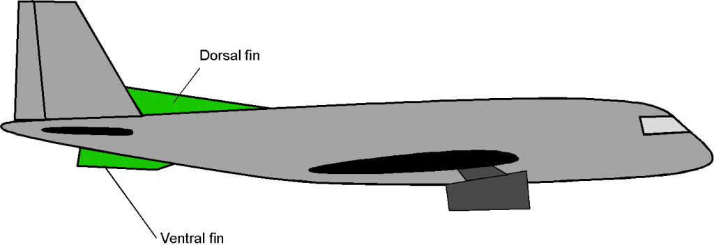
Indeed, dorsal or ventral fins are simple, lightweight structures and can be resized quickly and inexpensively during flight testing. They are often helpful in achieving the needed levels of directional stability for the airplane without having to embark on a complete redesign of the vertical tail to resolve deficiencies in the flight dynamics. The airplane in the photograph below, for example, suggests that additions were made after the first flights to improve its flight stability characteristics. In this case, adding so many separate vertical tail surfaces seems almost a design afterthought.
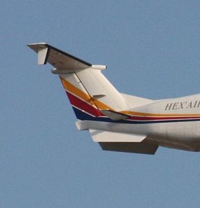
Evaluating Stability & Control Characteristics
The FAA’s regulations (and EASA’s Certification Specifications) outline comprehensive requirements to ensure an aircraft remains stable and controllable under all flight conditions that are part of its operational flight envelope. Stability and control standards include static and dynamic stability requirements, control surface effectiveness, and overall aircraft handling qualities. Aircraft must demonstrate positive static stability about all flight axes, ensuring they return to a steady state after disturbances. They must also show adequate dynamic stability, where pitch or other attitude oscillations damp out over time or can be damped with the regular use of flight controls. Control surfaces such as ailerons, elevators, and rudders must be effective throughout the flight envelope, providing sufficient authority for attitude and fight path management. Additionally, handling qualities must be predictable and manageable, with control forces and responses being well-balanced and coordinated to allow for pleasing and safe flight characteristics.
The stability and control certification process involves rigorous design and testing phases. Aircraft manufacturers conduct computational simulations, simulator tests, wind tunnel tests, and in-flight testing to ensure the airplane’s stability and control characteristics will be able to comply with regulatory standards. They must also provide comprehensive documentation of the results, including detailed test reports, data, and analysis, to the relevant aviation authority to demonstrate adherence to stability and control requirements. Continuous monitoring and periodic re-evaluation ensure that aircraft maintain compliance with these standards throughout their operational life.
Flight Testing
Flight testing is essential for validating design assumptions and ensuring the aircraft meets stringent safety and performance criteria. Flight testing to validate stability and control is a crucial phase in the development and certification of aircraft. It aims to ensure safe and predictable flight characteristics over the entire flight envelope. It involves a systematic approach to performing maneuvers and analyzing data to validate the aircraft’s performance against regulatory standards and design requirements. Needless to say, it is a lengthy and expensive part of the aircraft’s certification process.
Maneuvers conducted during flight testing include trim and static stability tests to assess how the aircraft responds to pitch, roll, and yaw changes, confirming it returns to its original state after disturbances. Dynamic stability tests involve inducing disturbances to excite the short-period and long-period oscillations to evaluate the aircraft’s damping and characteristics, usually as a function of speed (Mach number) and altitude. Control effectiveness tests assess the responsiveness of the ailerons, elevators, and rudders to ensure they provide sufficient control authority and operate normally and in the correct sense throughout the flight envelope.
Data analysis techniques during flight testing involve comprehensive instrumentation to record parameters such as airspeed, altitude, control surface positions, and aircraft accelerations. Time history analysis examines how these variables evolve during maneuvers, providing quantitative values of the aircraft’s stability characteristics. As previously discussed, frequency domain analysis assesses the aircraft’s response to control inputs regarding damping ratios and natural frequencies of oscillatory modes. Parameter estimation and statistical analysis refine mathematical models used in the simulator and validate the flight test values against theoretical predictions.
Control Effectiveness & Harmony
Control effectiveness refers to the ability of an aircraft’s control surfaces, including the ailerons, elevators, rudder, and flaps, to produce the desired changes in the flight path. Effectiveness is influenced by factors such as the size and shape of the control surfaces, the deflection angle, airflow, speed, and the overall aircraft configuration. Larger control surfaces generally provide greater control authority, allowing for more pronounced changes in attitude. Additionally, higher speeds improve control effectiveness from greater dynamic pressure, while lower speeds require additional systems like spoilers, flaps, or other high-lift devices to maintain control.
Control harmony deals with the balance and coordination between different control inputs, ensuring that the aircraft responds predictably and smoothly to pilot commands. Achieving control harmony involves ensuring that the forces needed to operate all control surfaces are well-balanced and that the aircraft responds proportionally to control inputs. For example, the effort required to move the ailerons, elevator, and rudder should be consistent to avoid excessive force requirements during maneuvers. Additionally, when rolling the aircraft with ailerons, coordinated use of the rudder helps prevent adverse yaw effects, resulting in smoother turns.
Overall, good control harmony means the effort and displacement required for the various control inputs are proportional and intuitive to the pilots. This proportionality reduces the likelihood of over-controlling in one flight axis. Balanced control forces and intuitive coordination among controls are essential for maintaining smooth and predictable aircraft behavior, and test pilots approach this using formal assessments. Poor control effectiveness or disharmony can lead to unpredictable aircraft behavior, increased pilot workload, and potentially hazardous flight conditions.
Handling Qualities Assessments
As part of the flight testing process, handling or flying qualities is used in the study and evaluation of an aircraft’s stability and control characteristics. It is a field where aircraft design, aerodynamics, physiology, psychology, and ergonomics intersect.[4] Assessments of handling qualities are critical to the flight of the aircraft and are related to the ease of controlling an airplane in steady flight and various types of maneuvers. The “ease” of controlling the aircraft will include the forces needed to be applied to the different controls that the pilot must move or otherwise actuate during flight.
Poor handling qualities can lead to pilot error, loss of control, and mishaps or accidents. Therefore, aircraft manufacturers and regulatory bodies greatly emphasize an aircraft’s handling qualities during its certification and operational phases. Test pilots and flight test engineers use the Cooper-Harper handling qualities rating scale to assess aircraft handling and flying qualities. The numerical scale ranges from 1 to 10, with a value of 1 indicating the best handling characteristics and a value of 10 being the worst, i.e., the aircraft is unflyable.
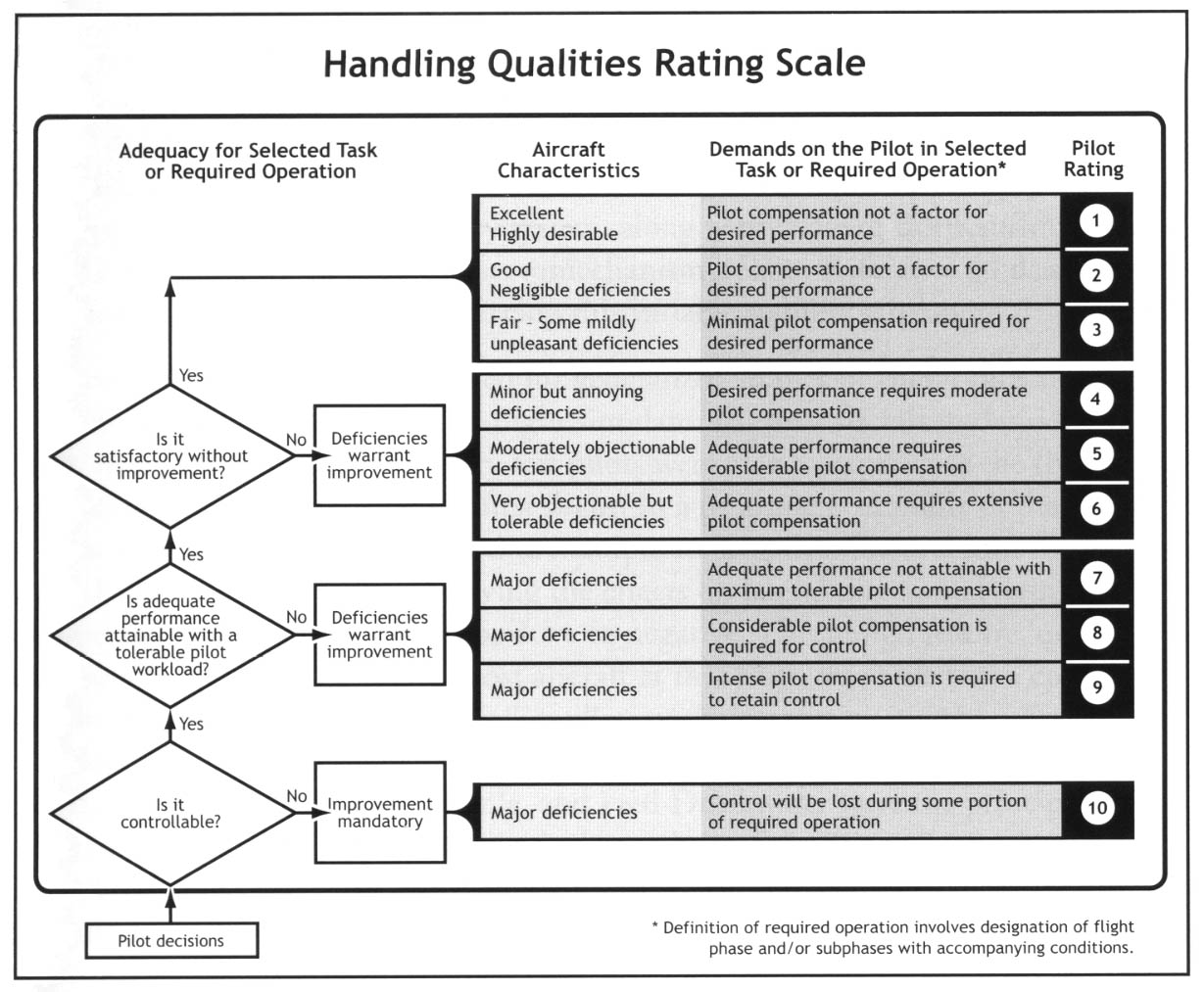
The scale is subjective, so several test pilots and engineers are usually used to evaluate aircraft handling qualities. Specific mission task elements (MTEs) are generally defined for the aircraft in question (based on its intended purpose), which are a set of “role-relatable” or representative flight tasks. The test pilots and flight test engineers then evaluate the aircraft’s handling qualities against these MTEs, amongst other criteria.
The handling qualities are judged not just by reference to the aircraft’s role but also by the MTE and the skill level expected of an average pilot. Usually, handling qualities assessments rated less than Level 3 are considered unacceptable for a modern aircraft, and changes to the aircraft and/or the flight control system will likely be required. Particular attention is usually focused on exploring deficient handling qualities in the form of pilot-induced oscillations (PIO) or, in general, the possibility of any Aircraft-Pilot Coupling (APC) effects. In addition, there are derivative MTEs used for specialist military flight operations such as air-to-air refueling, operations from ships, etc.
Stability Augmentation Systems
Stability Augmentation Systems (SAS) are sophisticated avionics and computers designed to enhance an aircraft’s stability and handling characteristics, particularly in adverse conditions or during critical phases of flight. These systems are integrated into the flight control system and use automatic adjustments to the flight control surfaces to maintain acceptable stability values during flight.
Key components of a SAS include air data sensors to provide critical information about airspeed, altitude, and other environmental conditions, angle of attack sensors, accelerometers, rate gyros, yaw dampers, pitch and roll stabilization systems, as well as other elements depending on the type of aircraft. Yaw dampers are crucial on jet airliners to prevent Dutch roll by automatically making rudder inputs. Pitch stabilization systems maintain the desired pitch attitude, while roll stabilization systems prevent unwanted roll movements by controlling ailerons or spoilers. Autopilot systems, which are not the same as a SAS, manage the aircraft’s flight path, including altitude, heading, and speed, based on pilot inputs or pre-programmed flight plans. Autopilots reduce the need for constant manual inputs from the pilot, allowing for more focused and safer flight operations, especially in turbulent air. A SAS is included as an integral part of the fly-by-wire systems used in modern military and civil aircraft, an example being shown in the figure below.
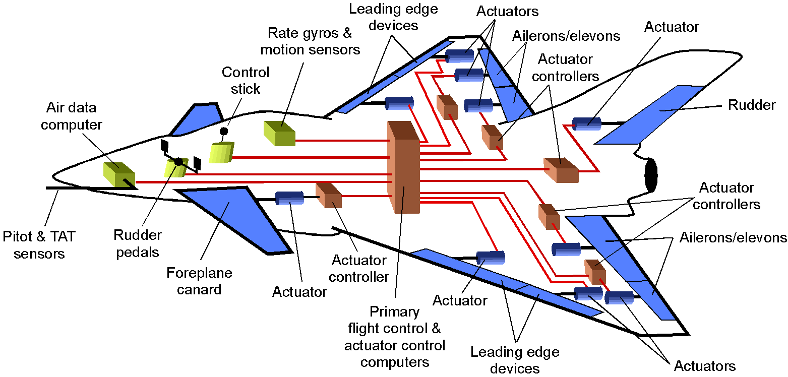
The operation of a SAS involves a holistic integration of sensors, control algorithms written in software, and either electrical or hydraulic actuators. Sensors continuously monitor various parameters like the aircraft’s attitude, angle of attack, and turn rate. Computers process this data in real-time to determine necessary adjustments to the control surfaces. Actuators then execute any needed adjustments, forming a feedback loop that ensures continuous, precise control of the aircraft’s stability and orientation. The flight control and SAS software are usually quadruply redundant and operated in parallel.
Despite their advantages, SAS also introduces specific challenges. The complexity and criticality of these systems necessitate preventative maintenance and regular checks. Pilots may also become overly dependent on automation, especially when flying airliners, which can degrade their manual flying skills over time. However, pilots can maintain their proficiency with proper training and practice, and most airline pilots fly manually when conditions permit or fly other airplanes.
Summary & Closure
Sufficient stability and control are crucial factors in the design of any flight vehicle. Aerospace engineers must understand the basics of stability and control to ensure safe and efficient flight. The term stability is initially viewed as static stability, which is the aircraft’s initial response to a disturbance, such as a gust of wind. If the aircraft returns to its original state after removing the disturbance, it is statically stable. For an airplane, static stability about all axes is necessary for safe flight and good handling, which is usually mandated during design.
Dynamic stability refers to the aircraft’s response over time to a disturbance. If the aircraft oscillates around its original trim state before returning to a stable state, it is said to be dynamically stable. Dynamic stability is explored and documented during flight testing, and changes to the design may be made if needed to improve its dynamic stability. Aerodynamic surfaces like ventral or dorsal fins, increasing the surface area and the resulting aerodynamic forces, may also be added to an aircraft to increase damping and improve stability characteristics.
Aircraft handling qualities refer to the ease and precision with which a pilot can control an aircraft to perform a specific task, such as maneuvering, landing, or following a particular type of flight path, e.g., an instrument approach. Good handling qualities are critical for safe and efficient flight operations, as they allow the pilot to maintain positive control of the aircraft in all flight conditions.
5-Question Self-Assessment Quickquiz
For Further Thought or Discussion
- Review and comment on the tail design for the Beech 1900 turboprop airplane.
- Can you fly a statically unstable aircraft? Explain carefully.
- During flight testing, it was found that a new military fighter airplane has a very pronounced spiral instability mode. Consider the options as to whether this is a problem and whether it should be mitigated.
- It is found during flight testing of an airplane that, under some conditions, the phugoid mode is mildly divergent. Discuss whether this is a problem or not.
- Besides PIO, do some research to learn more about Aircraft-Pilot Coupling (APC) events.
- If the yaw damper on a jet aircraft fails during flight, are there likely any issues of concern?
- Consider some types of handling qualities assessments that might be needed for an uncrewed aerial vehicle.
Other Useful Online Resources
To dive further into the stability and control of aircraft, visit the following websites:
- A great website covering many aspects of aircraft stability and control.
- A fantastic educational old film on the Secret of Flight 5: Stability and Control
- A nice set of course notes on stability and control published by Cornell University.
- A good website on aspects of stability and control from the piloting perspective.
- The author acknowledges his teacher, Arthur W. Babister. Dr. Babister was a flight dynamics engineer at the Blackburn Aircraft Company and contributed to the design of the Buccaneer fighter bomber and the Beverly transport airplane. He became a professor of aeronautical engineering at the University of Glasgow in 1965. Using his well-known book, "Aircraft Dynamic Stability and Response," he taught countless student engineers the intricacies of flight dynamics, always appreciating that it was not the most straightforward subject to master. ↵
- First given by Lanchester in his 1908 book titled Aerodonetics. ↵
- The term "Dutch roll," describing this particular dynamic response of an airplane in analogy with ice skating, was coined by Jerome C. Hunsaker in 1916. ↵
- Micael Carley, "Aircraft Stability and Control," University of Bath . ↵
