21 Momentum Equation
Introduction
The second physical principle used in deriving the governing equations that describe aerodynamic flows (or the flow of a fluid, in general) is the conservation of momentum, i.e., the application of Newton’s second law. This principle is one of the most important for solving aerodynamic motion because it allows solving problems involving the forces produced on or by flows, such as the lift and drag on a wing or the thrust produced by a jet or rocket engine.
From elementary physics, Newton’s second law is usually written as  , where
  is the force on the system,
  is the mass of the system, and
  is the resulting linear acceleration of the system. However, the most general form of Newton’s second law is when it is written in terms of the time rate of change of momentum, i.e.,
(1) 
where  is the total linear momentum in this case; naturally, there are analogous equations for angular momentum. Remember that, in reference to “momentum,” the meaning is that it refers to the momentum of something, whether it is a mass, a fluid element, or something else. Also, note that the plural of momentum is “momenta,” not “momentums.”
Learning Objectives
- Understand the principle of conservation of momentum when applied to a fluid.
- Be able to set up the most general form of the momentum equation for a fluid, including all sources of forces.
- Use the momentum and continuity equations to solve elementary flow problems.
- Understand the development of the Euler and Navier-Stokes equations.
Momentum Equation – Integral Approach
The objective is to apply the conservation of linear momentum principle to a flow to find a mathematical expression for the forces produced on a fluid flow in terms of the familiar macroscopic flow field variables, such as density  , velocity
  , and pressure,
  . Pressure comes into the problem of describing this behavior because any non-uniform pressure in a flow acting over an area can produce a force. Such non-uniform pressures are referred to as pressure gradients, as they cause an imbalance of forces on the flow, accelerating or decelerating it and thus altering its momentum.
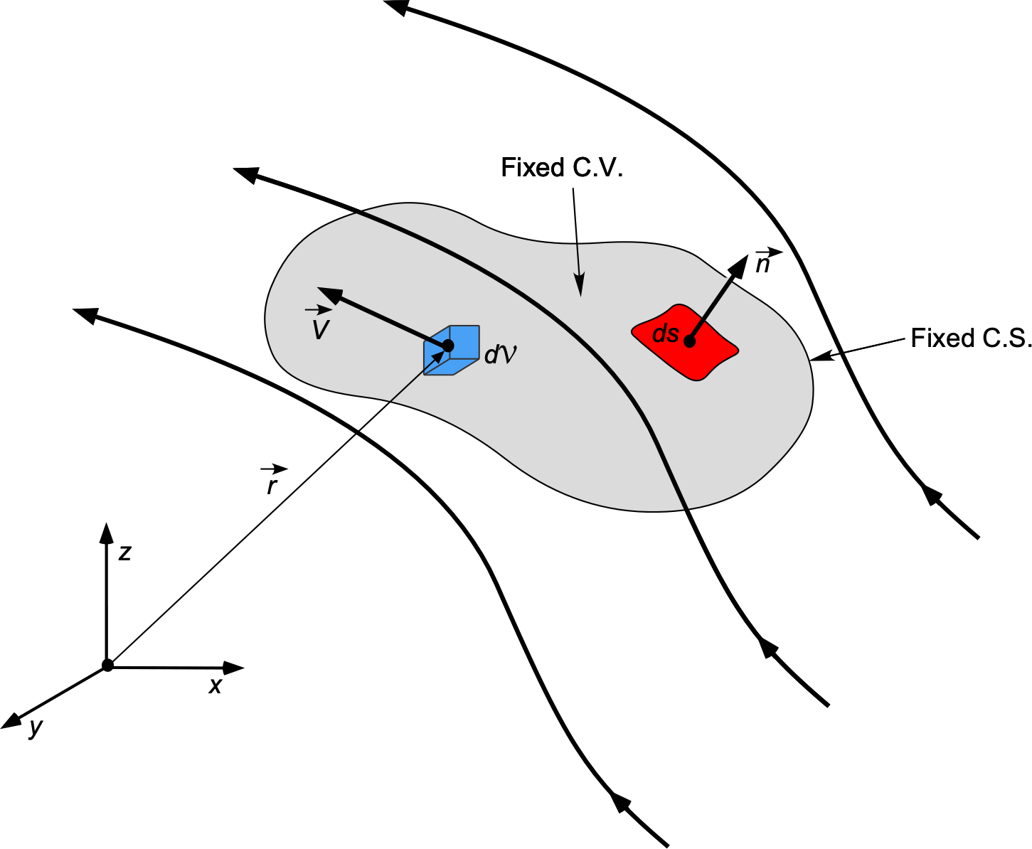
Flow Model
Consider the previously used control volume approach, as shown in the figure below. Recall that the control volume is abbreviated as “C.V.” and the control surface as “C.S.” The volume is assumed to be fixed in space, with the fluid moving through it; this is a fluid moving in an Eulerian modeling approach. In general, the forces on the air, as it flows through the C.V., will manifest from two sources, namely:
- Body forces: These include gravity, inertial accelerations (maybe even electromagnetic, electrostatic forces), etc., and may act on the fluid elements inside the C.V. The idea of a body force resulting from gravity was introduced when the hydrostatic equation was established, i.e.,
 .
. - Surface forces: Pressure and viscous shear stress act on the area of the control surface,
 , leading to forces.
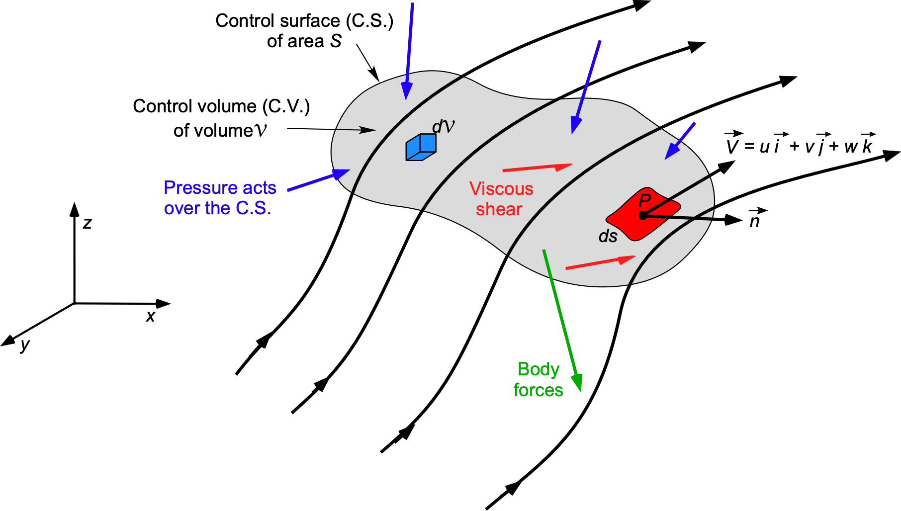
Pressure Forces
The pressure force acting on the elemental area  is
is  , where the negative sign indicates that the force is inward and in the opposite direction to the unit normal vector area, which always points outward by convention. Therefore, the total pressure force on the fluid inside the C.V. is the summation of the elemental forces over the entire C.S., i.e., the pressure force is given by
(2) 
Body Forces
Now consider the body forces, where  is defined as the net body force per unit mass exerted on the fluid inside
  . The body force on the elemental fluid volume
  is
is  , and the total body force is the summation over the volume , i.e.,
(3) 
An example of a body force is gravity. So in this case, the body force per unit mass is simply the acceleration under gravity, i.e.,  , so that in terms of the body force vector, then
  . By convention, the direction of
  is usually directed vertically upward, so the minus sign indicates that gravity is directed downward.
Viscous Forces
If the flow is viscous, and all fluids are viscous to a lesser or greater degree, then the viscous shear stresses  that arise over the C.S. will exert a surface force. These forces depend on the fluid’s viscosity and the velocity gradients in the flow, making it potentially difficult to evaluate such forces. Therefore, the viscous effects can be recognized but not yet evaluated. The total viscous force on the C.S. as it passes through the C.V. will be given by
(4) 
It is essential to understand that the actual quantitative evaluation of this integral may be complex and typically requires some effort, especially when turbulence is present. Nevertheless, its perpetual presence cannot be ignored.
Total Forces
Therefore, the total forces acting on the flow in the C.V. will be
(5) ![\begin{equation*} \vec{F} = \vec{F}_p + \vec{F}_b + \vec{F}_{\mu} = \underbrace{ -\oiint_{S} p \, d\vec{S}}_{\begin{tabular}{c} \scriptsize Pressure \\[-4pt] \scriptsize forces \end{tabular}} + \underbrace{ \oiiint_{{\cal V}} \varrho\, \vec{f}_b \, d{\cal {V}}}_{\begin{tabular}{c} \scriptsize Body \\[-4pt] \scriptsize forces \end{tabular}} + \underbrace{ \iint_{S} \tau \, d{\vec{S}}}_{\begin{tabular}{c} \scriptsize Viscous \\[-4pt] \scriptsize forces \end{tabular}} \end{equation*}](https://eaglepubs.erau.edu/app/uploads/quicklatex/quicklatex.com-bca982ad338204d3488bf80e9be81aff_l3.svg "Rendered by QuickLaTeX.com")
which will constitute the net force that must appear on the left-hand side of the final momentum equation.
Momentum Terms
Now consider the right-hand side of the momentum equation, i.e., the term that must describe the fluid’s time rate of change of momentum. There will be two contributions to this, namely:
- The net momentum flows out of the C.V. across the surface of area per unit of time.
- The time rate of momentum change inside will only occur if there are any unsteady fluctuations in the flow properties.
Consider the first term. At any point inside the C.V. or on the C.S., the flow velocity is . The mass flow across the element is given by  so the flow of momentum across will be
(6) 
The net flow of momentum out of the control C.V. over the C.S. is the sum of all the elemental contributions, i.e.,
(7) 
Now, consider the second term. The momentum of the fluid inside the element of volume will be  , and so the total momentum contained inside the C.V. at a given time is
(8) 
and its time rate of change (which can only result from unsteady flow fluctuations) will be
(9) 
Final Form of the Momentum Equation
Combining all the above equations into the form  gives an expression for momentum conservation in terms of the total forces and time rate of change of momentum of the flow as it sweeps through the C.V., i.e.,
(10) 
which is another “star” governing equation. In other words, Eq. 10 states that Total Forces = Body Forces + Pressure Forces + Viscous Forces = Time rate of change of momentum inside from any unsteadiness in the flow + Net flow of momentum out of across the C.S. of area per unit time. This general equation applies to any flow, whether compressible or incompressible, viscous or inviscid, and so on.
Equation 10 is the momentum equation in its integral form, first established by Leonhard Euler. It will be apparent that it is a vector equation, so three scalar equations are rolled into one, i.e., one equation for each coordinate direction. If  , then
(11) ![\begin{eqnarray*} F_x & = & \frac{\partial}{\partial t}\oiiint_{\cal{V}} \varrho \, u \, d {\cal{V}} + \oiint_S (\varrho \, \vec{V} \bigcdot d\vec{S}) u \\[6pt] F_y & = & \frac{\partial}{\partial t}\oiiint_{\cal{V}} \varrho \, v \, d {\cal{V}} + \oiint_S (\varrho \, \vec{V} \bigcdot d\vec{S}) v \\[6pt] F_z & = & \frac{\partial}{\partial t}\oiiint_{\cal{V}} \varrho \, w \, d {\cal{V}} + \oiint_S (\varrho \, \vec{V} \bigcdot d\vec{S}) w \end{eqnarray*}](https://eaglepubs.erau.edu/app/uploads/quicklatex/quicklatex.com-41bf78a643e570f5887c30e75916574d_l3.svg "Rendered by QuickLaTeX.com")
What are the units of momentum?
When we speak of “momentum,” we mean the momentum of something. Momentum is a vector quantity, so it has both magnitude and direction. If denotes mass and denotes velocity, then the translational momentum is . Therefore, in terms of base dimensions
![\[ \left[ m \vec{V} \right] = \rm M \, L \, \rm T^{-1} = \left( \rm M \, L \, T^{-2} \right) \rm T \]](https://eaglepubs.erau.edu/app/uploads/quicklatex/quicklatex.com-097c200b26da70d823b8391f83e092e8_l3.svg "Rendered by QuickLaTeX.com")
noting that the units inside the parentheses represent a force. Therefore, in the SI system, the units of the translational momentum of a fluid will be kg m s , which is also equivalent to a Newton-second, i.e., N s. In the USC system, the units of momentum will be slug ft s, which is also equivalent to a pound-second, i.e., lb s.
Simplifications to the Momentum Equation
As in the use of the continuity equation for practical problem solving, the apparent complexity of the general form of the momentum equation can be simplified by making justifiable assumptions; the advantage is that the solutions to the resulting sets of governing equations (mass, momentum, and energy) become commensurately easier. Remember that any assumptions must be justified, which may require information from an experiment or a judgment call, i.e., based on experience and expertise. Experience is acquired through repeated problem-solving, i.e., starting with exemplar problems in the classroom and then doing many more on one’s own.
Consider, for example, a steady flow. In this case,  , so the reduced form of the momentum equation becomes
(12) 
If the flow is inviscid, then  . Therefore, the momentum equation simplifies to
(13) 
If the flow is also incompressible, then is constant and can be factored out, i.e.,
(14) 
If body forces can be neglected, then the pressure forces must balance the momentum flux, so that
(15) 
Alternatively, if pressure forces are negligible or the momentum terms are much greater than the pressure terms, then the momentum equation becomes
(16) 
Two-Dimensional Forms of the Momentum Equation
A two-dimensional simplification is often suitable for many practical applications, particularly in external flows or flows confined by walls. Volume integrals reduce to area integrals per unit depth, and surface integrals reduce to line integrals around the boundary of a planar control surface.
The component form of the momentum equation for a two-dimensional, steady, incompressible, inviscid flow becomes
(17) ![\begin{eqnarray*} F_x & = & \oiint_S \left[ \varrho \left( \vec{V} \bigcdot d\vec{S} \right) u + p \, \hat{i} \bigcdot d\vec{S} \right] \\[6pt] F_y & = & \oiint_S \left[ \varrho \left( \vec{V} \bigcdot d\vec{S} \right) v + p \, \hat{j} \bigcdot d\vec{S} \right] \end{eqnarray*}](https://eaglepubs.erau.edu/app/uploads/quicklatex/quicklatex.com-ef00f0bc0d381da7a3bd8c5cc2d6a74d_l3.svg "Rendered by QuickLaTeX.com")
These latter equations include both momentum flux and pressure forces. If pressure forces are negligible, the expressions reduce further to
(18) ![\begin{eqnarray*} F_x & = & \oiint_S \varrho \left( \vec{V} \bigcdot d\vec{S} \right) u \\[6pt] F_y & = & \oiint_S \varrho \left( \vec{V} \bigcdot d\vec{S} \right) v \end{eqnarray*}](https://eaglepubs.erau.edu/app/uploads/quicklatex/quicklatex.com-75bd6e047c609a128049a74564fa9025_l3.svg "Rendered by QuickLaTeX.com")
For a control volume with uniform properties at the inlet and outlet and negligible contributions from the other surfaces, these simplify further to
(19) 
where  is the mass flow rate through the control volume, and
  ,
,  are the changes in velocity components.
One-Dimensional Forms of the Momentum Equation
In the case of a one-dimensional flow, where the velocity vector is aligned with the  -axis and properties are uniform over the inlet and outlet cross sections, the momentum equation becomes
(20) 
which may be written as
(21) 
Further neglecting pressure forces, the momentum equation simplifies to
(22) 
or in terms of the mass flow rate, then
(23) 
where  . These one-dimensional forms are commonly used in applications when the flow is nearly unidirectional and cross-sectional variations in the flow dimensions are small.
Learning the Exemplars
The extent to which the momentum equation can be simplified depends on the problem’s complexity and the strength of the justifications for each assumption. Learning to make these simplifications effectively comes from studying classic examples in fluid dynamics. A structured approach, starting with fundamental problems and progressively working up to more complex scenarios, provides a solid foundation for understanding.
Beyond textbook examples, applying fluid dynamics concepts to real-world problems and using simulation software can significantly enhance comprehension. Computational tools enable a deeper exploration of flow behavior, facilitating the visualization and analysis of various scenarios. Additionally, numerous online resources, including open-access courses and materials from educational institutions, provide valuable opportunities for further study and practice.[1]
Check Your Understanding #1 – Force on a converging duct or nozzle
Reduce the general form of the momentum equation to a form suitable for application to the steady, compressible, one-dimensional flow of air through a converging duct (often called a contraction) of circular cross-section, i.e., a nozzle, as shown below.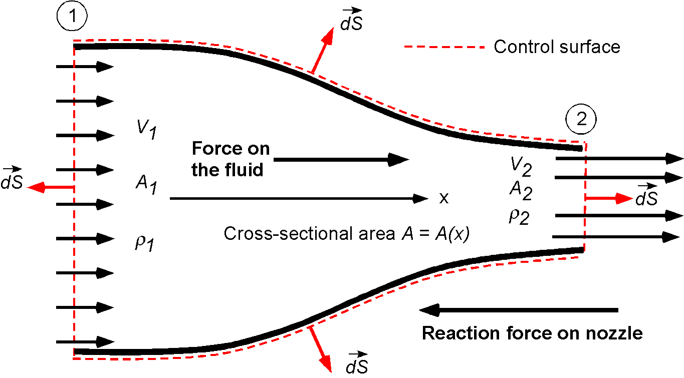
Show solution/hide solution.
Proceed first by sketching the nozzle problem, showing the control surface, and annotating the inlet and outlet conditions appropriately, not only with what is known but also with what is unknown. In this case, the net pressure force exerted by the nozzle on the fluid needs to be determined. The flow is assumed to be steady, so . The fluid is air, which has a relatively low density, and there is no change in elevation from one side of the nozzle to the other; therefore, it is possible to neglect all body forces, including the effects of gravity.
As previously derived, the general form of the momentum equation is
![\[ \oiiint_{\cal{V}} \varrho \, \vec{f} _b \, d{\cal{V}} -\oiint_S p \, d\vec{S} + \vec{F}_{\mu} = \frac{\partial}{\partial t}\oiiint_{\cal{V}} \varrho \, \vec{V} \, d {\cal{V}} + \oiint_S (\varrho \, \vec{V} \bigcdot d\vec{S}) \vec{V} \]](https://eaglepubs.erau.edu/app/uploads/quicklatex/quicklatex.com-b6fc38d33c174b30a5eef7e17b1b32cf_l3.svg "Rendered by QuickLaTeX.com")
The reduced form for the assumptions made that the flow is steady without body forces leads to
![\[ - \oiint_S p \, d\vec{S} + \vec{F}_{\mu} = \oiint_S (\varrho \, \vec{V} \bigcdot d\vec{S}) \vec{V} \]](https://eaglepubs.erau.edu/app/uploads/quicklatex/quicklatex.com-2c375b07c599259a6091bdc57e539872_l3.svg "Rendered by QuickLaTeX.com")
The left-hand side can be written as
![\[ -\iint_{A_1} p \, d\vec{S} - \iint_{A_2} p \, d\vec{S} + \underbrace{\iint_{\rm Walls} \!\! \!-p \, d\vec{S} + \vec{F}_{\mu} }_{F_x} \]](https://eaglepubs.erau.edu/app/uploads/quicklatex/quicklatex.com-a06a477a26f6fc81a34162cb993252cc_l3.svg "Rendered by QuickLaTeX.com")
In this case, the force on the fluid,  , which changes its momentum, needs to be determined; this is the unknown. Notice that this force can include both pressure forces and viscous forces. There is also an equal and opposite force on the nozzle, denoted as
  , which must ultimately be determined. Therefore, the momentum equation, in this case, is
![\[ F_x - \iint_{A_1} p \, d\vec{S} - \iint_{A_2} p \, d\vec{S} = \oiint_S (\varrho \, \vec{V} \bigcdot d\vec{S}) \vec{V} \]](https://eaglepubs.erau.edu/app/uploads/quicklatex/quicklatex.com-f9153f537c6d72a9b8480e3ad1c4b03d_l3.svg "Rendered by QuickLaTeX.com")
The flow can be assumed to be one-dimensional, meaning that the flow properties change only in one dimension. This assumption simplifies the solution process while still being realistic. With the one-dimensional assumption, then
![\[ F_{x} + p_1 A_1 - p_2 A_2 = \left( \varrho_2 A_2 V_2^2 - \varrho_1 A_1 V_1^2 \right) \]](https://eaglepubs.erau.edu/app/uploads/quicklatex/quicklatex.com-7fd149fb4e5667f3ddf9069a01d44c04_l3.svg "Rendered by QuickLaTeX.com")
noting the signs of the term on the first pressure integral over  and remembering that
  always points out of the control volume by convention. Also, the continuity of the flow means that
![\[ \varrho_1 A_1 V_1 = \varrho_2 A_2 V_2 \]](https://eaglepubs.erau.edu/app/uploads/quicklatex/quicklatex.com-2d530af2bc0ad38292a1ba18e424b36f_l3.svg "Rendered by QuickLaTeX.com")
So, the final form of the momentum equation for this problem becomes
![\[ F_{x} = (p_2 A_2 - p_1 A_1) + \varrho_1 A_1 V_1 \left( V_2 - V_1 \right) \]](https://eaglepubs.erau.edu/app/uploads/quicklatex/quicklatex.com-adef63884a3e3fb9659cdff5cbaf5a0c_l3.svg "Rendered by QuickLaTeX.com")
This force will be negative, i.e., to the left. The fact that this force is in the backward direction (opposite to the flow direction) is somewhat counterintuitive because momentum is being added to the fluid as it passes through the nozzle. But if a person is holding the nozzle, they must apply a forward force reaction while keeping it in place to prevent it from moving backward. This reaction force is
![\[ R_x = -F_x \]](https://eaglepubs.erau.edu/app/uploads/quicklatex/quicklatex.com-9ca5551945a8d745c1d42f9366fad076_l3.svg "Rendered by QuickLaTeX.com")
which will be to the right. Notice also that this problem involves velocities and pressures. However, the Bernoulli equation(as discussed in the next chapter) cannot be applied to this problem because there are viscous losses as the fluid passes through the nozzle. However, the continuity equation applies to any fluid flow, whether viscous or inviscid, and thus applies in this case, as does the momentum equation.
Check Your Understanding #2 – Force on an engine test stand
A static thrust stand is designed for testing a jet engine. The following conditions are expected for a typical test: intake air velocity = 200 m/s, exhaust gas velocity = 500 m/s, intake and exit cross-sectional areas = 1 m , intake static pressure = -22.5 kPa (= 78.5 kPa absolute), intake static temperature = 268K, exhaust static pressure = 0 kPa (101 kPa absolute). Estimate the thrust reaction force to design the test stand to carry, if it must have a safety factor of 3.
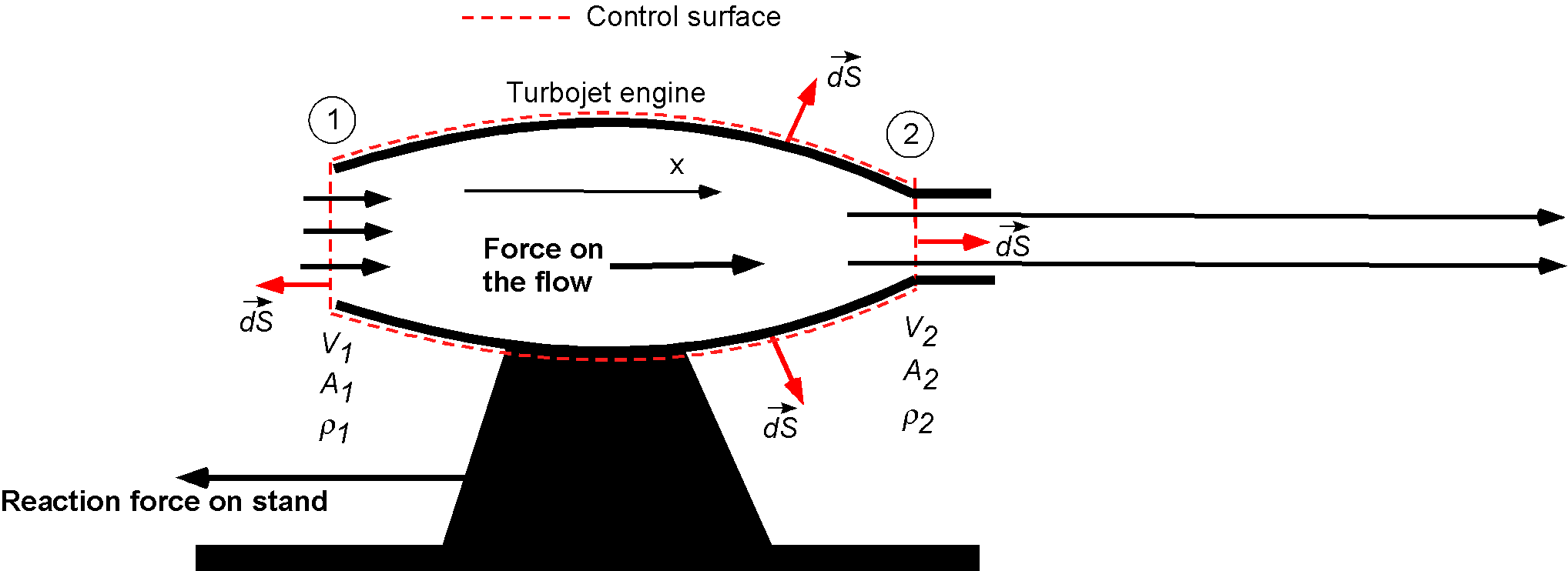
Show solution/hide solution.
Assume that the inlet is identified as station 1 and the outlet as station 2. The density of the air at the inlet can be found using
![\[ \varrho_1 = \frac{p_1}{R T_1} = \frac{78.5 \times 10^3}{(287)(268)} = 1.0206 ~\mbox{kg m${^{-3}}$} \]](https://eaglepubs.erau.edu/app/uploads/quicklatex/quicklatex.com-c460bbdfc789d32017d45e1fd2164d09_l3.svg "Rendered by QuickLaTeX.com")
From continuity considerations (assume 1-dimensional, steady flow), then
![\[ \varrho_1 A_1 V_1 = \varrho_2 A_2 V_2 = \overbigdot{m} = 204.12~\mbox{kg s$^{-1}$} \]](https://eaglepubs.erau.edu/app/uploads/quicklatex/quicklatex.com-a07a728270a2591642a184a344180931_l3.svg "Rendered by QuickLaTeX.com")
If the flow is additionally assumed to be inviscid and there are no gravitational effects, then  , and the relevant form of the momentum equation is
![\[ - \oiint_S p \, d\vec{S} = \varrho \oiint_S ( \vec{V} \bigcdot d\vec{S}) \vec{V} \]](https://eaglepubs.erau.edu/app/uploads/quicklatex/quicklatex.com-26772faa8c8be02a99825c739af46968_l3.svg "Rendered by QuickLaTeX.com")
The pressure integral on the left-hand side is
![\[ \oiint_S p \, d\vec{S} = \iint_{\rm Inlet} p \, d\vec{S} + \iint_{\rm Outlet} p \, d\vec{S} \iint_{\rm Engine} p \, d\vec{S} \]](https://eaglepubs.erau.edu/app/uploads/quicklatex/quicklatex.com-2fef933dc08b19ecae9894925bd202ea_l3.svg "Rendered by QuickLaTeX.com")
or
![\[ -\oiint_S p \, d\vec{S} = - \iint_{A_1} p \, d\vec{S} - \iint_{A_2} p \, d\vec{S} - F \]](https://eaglepubs.erau.edu/app/uploads/quicklatex/quicklatex.com-61c3404a59f22bdc41808fb1532abf7c_l3.svg "Rendered by QuickLaTeX.com")
where  is the force of the engine on the fluid. Assuming one-dimensional flow gives
![\[ -F + p_1 A_1 - p_2 A_2 = \overbigdot{m} ( V_2 - V_1 ) \]](https://eaglepubs.erau.edu/app/uploads/quicklatex/quicklatex.com-c68a173b340cfb48c4d388d0db79a233_l3.svg "Rendered by QuickLaTeX.com")
noting the signs of the terms, and remembering that always points out of the control volume, or
![\[ F = -p_1 A_1 + p_2 A_2 + \overbigdot{m} ( V_2 - V_1 ) \]](https://eaglepubs.erau.edu/app/uploads/quicklatex/quicklatex.com-d8f2ebdc40c4269ff94d0ab464645781_l3.svg "Rendered by QuickLaTeX.com")
noting that =  . Finally, substituting the known values gives
(24) 
For the conditions stated, the residual force on the fluid must be 83,736 N in the direction of fluid flow, and the reaction force on the test stand will be in the opposite direction. Because there is a factor of safety requirement of 3, the force to which the stand should be designed is about 251 kN.
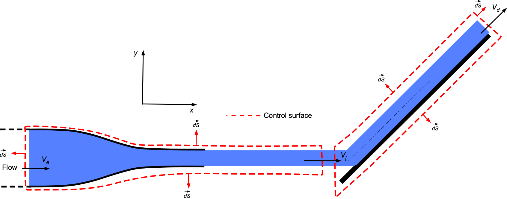
Check Your Understanding #3 – Force on an angled plate
Water ( = 1.94 slug ft
 ) flows at a mass flow rate of = 6.0 slug s through a nozzle of circular cross-section with an entrance diameter
  in and an exit diameter of
  in. The water jet then hits an angled plate with a circular groove, where it is deflected while also increasing in its circular cross-section, as shown in the figure below.
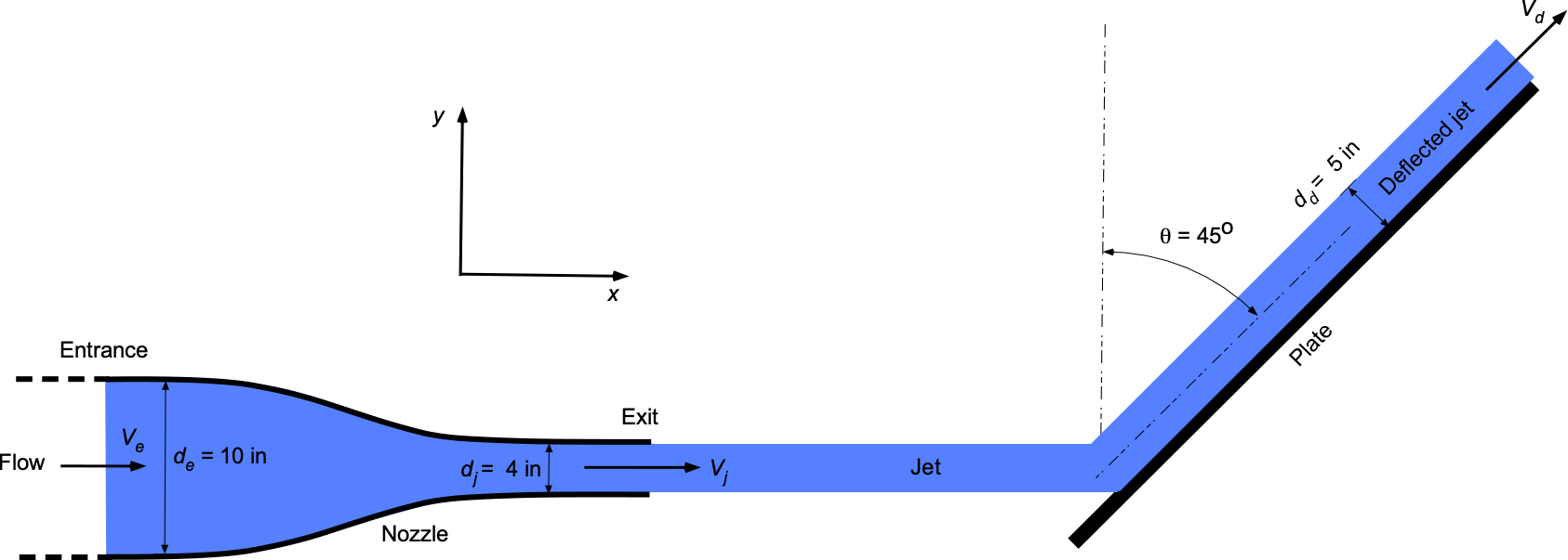
- Draw an appropriate control surface and volume with annotations to analyze this problem.
- Determine the velocity of the water as it enters and exits the nozzle.
- Determine the velocity of the water in the deflected jet.
- Determine the magnitude and direction of the force on the plate caused by the water jet.
Show solution/hide solution.
1. The appropriate control surface and volume, along with annotations, are shown below for the analysis of this problem.
2. This part of the problem requires the use of the continuity equation in its one-dimensional form, i.e.,
![\[ \overbigdot{m} = \varrho_w \ A_e \ V_e = \varrho_w \ A_j \ V_j \]](https://eaglepubs.erau.edu/app/uploads/quicklatex/quicklatex.com-392424fa6f3b147a28e03d3dc5c9b2ee_l3.svg "Rendered by QuickLaTeX.com")
The entrance area,  , is
, is
![\[ A_e = \frac{\pi d_e^2}{4} = \frac{\pi (10.0/12.0)^2}{4} = 0.5454~\mbox{ft${^{2}}$} \]](https://eaglepubs.erau.edu/app/uploads/quicklatex/quicklatex.com-a7763b05a3540e0c625b516a80adabc4_l3.svg "Rendered by QuickLaTeX.com")
Therefore, the entrance velocity is
![\[ V_e = \frac{\overbigdot{m}}{ \varrho_w \ A_j} = \frac{6.0}{1.94 \times 0.5454} = 5.67~\mbox{ft s$^{-1}$} \]](https://eaglepubs.erau.edu/app/uploads/quicklatex/quicklatex.com-429791c0e5a5b09a19adde28771340b0_l3.svg "Rendered by QuickLaTeX.com")
The exit jet area,  , is
, is
![\[ A_j = \frac{\pi d^2}{4} = \frac{\pi (4.0/12.)^2}{4} = 0.0873~\mbox{ft${^{2}}$} \]](https://eaglepubs.erau.edu/app/uploads/quicklatex/quicklatex.com-c7a85bd7f3668db8ae4044b2859ffb65_l3.svg "Rendered by QuickLaTeX.com")
Therefore, the exit jet velocity is
![\[ V_j = \frac{\overbigdot{m}}{ \varrho_w \ A_j} = \frac{6.0}{1.94 \times 0.0873} = 35.43~\mbox{ft s$^{-1}$} \]](https://eaglepubs.erau.edu/app/uploads/quicklatex/quicklatex.com-6cb031574e4056301fd72b2c45243fac_l3.svg "Rendered by QuickLaTeX.com")
3. The velocity  of the water in the deflected jet can be found using continuity, i.e.
![\[ \overbigdot{m} = \varrho_w \ A_d \ V_d \]](https://eaglepubs.erau.edu/app/uploads/quicklatex/quicklatex.com-eea725ac508071743b7d368a137f9a13_l3.svg "Rendered by QuickLaTeX.com")
The deflected jet area  is
is
![\[ A_d = \frac{\pi d_d^2}{4} = \frac{\pi (5.0/12.0)^2}{4} = 0.1364~\mbox{ft${^{2}}$} \]](https://eaglepubs.erau.edu/app/uploads/quicklatex/quicklatex.com-92e3efe4781d6f16aa5d84633f317c3c_l3.svg "Rendered by QuickLaTeX.com")
Therefore, the deflected jet velocity is
![\[ V_d = \frac{\overbigdot{m}}{\varrho_w \ A_d} = \frac{6.0}{1.94 \times 0.1364} = 22.67~\mbox{ft s$^{-1}$} \]](https://eaglepubs.erau.edu/app/uploads/quicklatex/quicklatex.com-eebef9d6702de8ababa8c7968151be4f_l3.svg "Rendered by QuickLaTeX.com")
4. The applicable form of the momentum equation is
![\[ \vec{F}= \overbigdot{m} \, \Delta \vec{V} \]](https://eaglepubs.erau.edu/app/uploads/quicklatex/quicklatex.com-e65644cbde2859c469ff8d9c87561013_l3.svg "Rendered by QuickLaTeX.com")
We can ignore all pressure forces because the plate is surrounded by free air at ambient conditions, so there is no pressure force on the control volume. In scalar form, because we have forces in two directions, then
![\[ F_x = \overbigdot{m} \ \Delta V_x \quad \mbox{and} \quad F_y = \overbigdot{m} \ \Delta V_y \]](https://eaglepubs.erau.edu/app/uploads/quicklatex/quicklatex.com-9496a3355521178845f33e64c5e137d5_l3.svg "Rendered by QuickLaTeX.com")
In the direction, the force on the fluid is
![\[ F_x = \overbigdot{m} \ \Delta V_x \]](https://eaglepubs.erau.edu/app/uploads/quicklatex/quicklatex.com-47d2080dec4bdd4e61d375b765b2e2df_l3.svg "Rendered by QuickLaTeX.com")
where  is the change in the flow velocity in the
  direction. Therefore,
![\[ F_x = \overbigdot{m} \left( V_d \ \cos \theta - V_j \right) = 6.0 \left( 22.67 \ \cos 45^{\circ} - 35.43 \right) = -116.4~\mbox{lb} \]](https://eaglepubs.erau.edu/app/uploads/quicklatex/quicklatex.com-0376a8caf0c9560839b1f3dd56d690cd_l3.svg "Rendered by QuickLaTeX.com")
In the  direction, the force on the fluid is
![\[ F_y = \overbigdot{m} \ \Delta V_y \]](https://eaglepubs.erau.edu/app/uploads/quicklatex/quicklatex.com-f9fe701a6fb0f79d1cca3d848464f630_l3.svg "Rendered by QuickLaTeX.com")
where  is the change in the flow velocity in the direction. Therefore,
![\[ F_y = \overbigdot{m} \left( V_j \ \sin \theta - 0 \right) = 6.0 \left( 22.67 \ \sin 45^{\circ} - 0.0 \right) = 96.2~\mbox{lb} \]](https://eaglepubs.erau.edu/app/uploads/quicklatex/quicklatex.com-a1f48033fea9c38521e1ee062b44b10c_l3.svg "Rendered by QuickLaTeX.com")
If the force on the fluid is
![\[ \vec{F} = -116.4 \ \, \vec{i} + 96.2 \, \vec{j}~~\mbox{lb} \]](https://eaglepubs.erau.edu/app/uploads/quicklatex/quicklatex.com-2f4bbe33b8ce0b0d2481b6cd615cb13d_l3.svg "Rendered by QuickLaTeX.com")
Then, the reaction force on the plate is
![\[ \vec{R} = 116.4\ \, \vec{i} - 96.2 \ \, \vec{j}~~\mbox{lb} \]](https://eaglepubs.erau.edu/app/uploads/quicklatex/quicklatex.com-7a71b8ddadb51c0ad09af10ff58b6676_l3.svg "Rendered by QuickLaTeX.com")
which is to the right and downward.
Angular Momentum
For most fluid mechanics problems, especially in incompressible flows, consideration of linear momentum is sufficient because rotational effects are either negligible or irrelevant to the problem’s primary focus. Angular momentum effects tend to be evident in cases with strong rotational characteristics or where torque calculations are required. For example, in turbomachinery, such as pumps, turbines, or compressors, the angular momentum equation is essential for analyzing the torque and rotational energy transfer within the control volume. Furthermore, specific fluid flow problems, such as vortices, involve the conservation of angular momentum as fluid particles follow circular or spiral paths. In these cases, the analysis can often use angular momentum principles to derive velocity profiles or understand the flow behavior.
The basic flow model used for angular momentum is shown in the figure below. To include angular momentum in the momentum equation, the angular momentum (moment of momentum), i.e.,  , over a control volume
  is defined by
(25) 
where is the fluid density,  is the position vector from some reference, and is the velocity vector. The net time rate of change of angular momentum from the control volume can be expressed as
(26) 
The first term represents the local (time) rate of change of momentum within , and the second term accounts for the angular momentum flux across the control surface .
To balance the angular momentum, it is necessary to consider the external moments acting on the fluid inside the C.V. These moments include:
- Moment of body forces. If
 is the body force per unit mass (e.g., gravity), the moment from the body forces is given by
(27)

- Moment of surface forces. The pressure and viscous stresses on the surface contribute to the surface moment. Regarding pressure , the moment contribution is
(28)

where
is the outward-directed unit normal vector area. - The moment caused by the stresses. The viscous contribution
 represents the integrated moment from viscous stresses, i.e., the integral of the moments caused by the shear stresses acting over the C.S.
 - A torque (which is also a moment) from mechanical sources. In many cases, the angular momentum of a fluid is caused by the action of a mechanical device driven through a shaft, such as a pump, propeller, or rotor. Therefore, in this case,
 represents this torque on the fluid.
With these definitions, the angular momentum balance for the fluid in a control volume becomes
(29) 
Substituting the expressions for the moments gives
(30) 
The complete angular momentum equation, combining the rate of change of angular momentum and the moments, is
(31) 
This equation states that the net external moment  acting on the control volume is balanced by the rate of change of angular momentum within and the flux of angular momentum across the surface .
Notice that the foundation of the angular momentum equation is the  . This term represents the angular momentum per unit volume, also known as the moment of momentum density.
Linear Momentum Equation from the RTE
Recall that the Reynolds Transport Equation (RTE) can be expressed as
(32) ![\begin{equation*} \underbrace{\frac{D}{Dt} \oiiint_{\mathrm{sys}} \beta \, \varrho \, d\mathcal{V}}_{\begin{tabular}{c} \scriptsize Time rate of \\[-3pt] \scriptsize change of $B$ \\[-3pt] \scriptsize inside the system.\end{tabular}} = \underbrace{\frac{\partial}{\partial t} \oiiint_{\mathcal{V}} \beta \, \varrho \, d\mathcal{V}}_{\begin{tabular}{c} \scriptsize Time rate \\[-3pt] \scriptsize of change of $B$ inside\\[-3pt] \scriptsize the control volume.\end{tabular}} + \underbrace{\oiint_{S} \beta \, \varrho ( \vec{V}_{\mathrm{rel}} \bigcdot d\vec{S}) }_{\begin{tabular}{c} \scriptsize Rate at which $B$ is \\[-3pt] \scriptsize leaving through the \\[-3pt] \scriptsize control surface.\end{tabular} } \end{equation*}](https://eaglepubs.erau.edu/app/uploads/quicklatex/quicklatex.com-3c356f70b229b863763a21a72c19cc73_l3.svg "Rendered by QuickLaTeX.com")
In the case of momentum, then  , and for the system, any change in momentum is equivalent to a force, so
(33) 
where is the net force acting on the fluid in the C.V., and  is the substantial derivative. Recall that the net force depends on body forces, pressure forces, and viscous forces, i.e.,
(34) 
Therefore, the RTE becomes
(35) 
which is the linear momentum equation. Remember that the momentum equation is a vector equation.
For steady flow, the momentum equation becomes
(36) 
For incompressible flow where is constant, the density term can be taken outside of the integral to get
(37) 
Momentum Equation – Differential Form
The momentum equations in differential form are called the Euler equations. In 1757, Leonhard Euler published his foundational work on the dynamics of fluids, which included the differential form of the momentum equations now known as the Euler equations. The Euler equations describe the motion of an inviscid fluid, i.e., a fluid of limitingly diminishing viscosity. Euler’s work laid the groundwork for later developments in fluid mechanics, including the Navier-Stokes equations, which extend the Euler equations to include viscosity effects.
Classic Approach
To derive the Euler equations, the classic approach is to apply the principles of conservation of momentum to a small differential fluid element. Consider a small fluid element in a Cartesian coordinate system with dimensions  ,
,  , and
, and  , as shown in the figure below. The volume of this fluid element is
  .
.
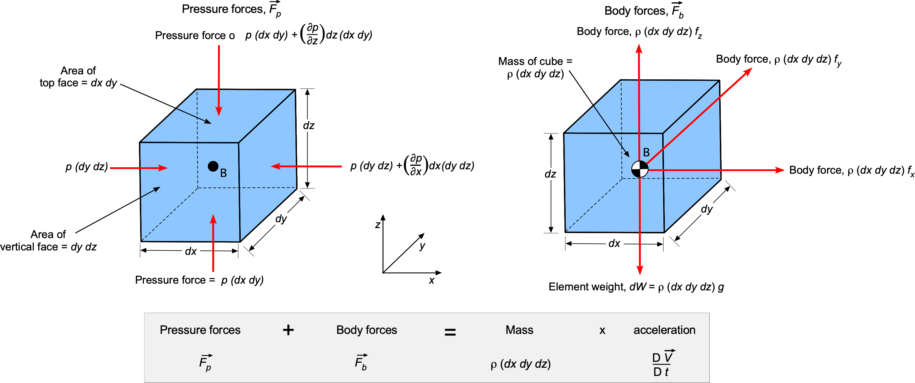
Pressure Forces
Consider the pressure forces in the direction, i.e., on the – face of area
  . Let
. Let  be the change of pressure with respect to . The net pressure force in the direction is
(38) 
The pressure gradient term, as a pressure force per unit mass, appeared previously in the derivation of the hydrostatic equation. Similarly, for the and directions, the net pressure forces are
(39) 
Therefore, the net resultant pressure force on the entire fluid element is
(40) ![\begin{eqnarray*} d\vec{F} & = & dF_x \, \vec{i} + dF_y \, \vec{j} + dF_z \, \vec{k} = -\left( \frac{\partial p}{\partial x} \, \vec{i} + \frac{\partial p}{\partial y} \, \vec{j} + \frac{\partial p}{\partial z} \, \vec{k} \right) dx \, dy \, dz \nonumber \\[6pt] & = & -\nabla p \, (dx \, dy \, dz ) = -\nabla p \, d {\mathcal{V}} \end{eqnarray*}](https://eaglepubs.erau.edu/app/uploads/quicklatex/quicklatex.com-2b95fcff99555f71b8b79e08d2d958a5_l3.svg "Rendered by QuickLaTeX.com")
Body Forces
Body forces per unit mass acting on the element can be described as
(41) 
Gravity is an omnipresent body force, i.e.,  . It is often useful to isolate and take the term outside of other body force terms, i.e.,
(42) 
Momentum Terms
According to Newton’s second law, this force is equal to the time rate of change of momentum of the fluid element, i.e.,
(43) 
where is the substantial derivative. Therefore,
(44) 
Cancelling out  and rearranging gives
(45) 
Similarly, for the and directions, then
(46) 
Final Form
Combining the previous results gives the Euler equations for an inviscid fluid, i.e.,
(47) ![\begin{equation*} \boxed{ \begin{aligned} &\frac{Du}{Dt} = -\frac{1}{\varrho} \frac{\partial p}{\partial x} + f_x \\[6pt] &\frac{Dv}{Dt} = -\frac{1}{\varrho} \frac{\partial p}{\partial y} + f_y \\[6pt] &\frac{Dw}{Dt} = -\frac{1}{\varrho} \frac{\partial p}{\partial z} + (f_z - g) \end{aligned} }^{~*} \end{equation*}](https://eaglepubs.erau.edu/app/uploads/quicklatex/quicklatex.com-5a7cff740bd1bf5e98d7de25221ffd6d_l3.svg "Rendered by QuickLaTeX.com")
In vector form, these equations can be written as
(48) 
Expanding out the substantial derivatives, then in the (long-handed) scalar form, they are
(49) ![\begin{eqnarray*} \frac{\partial u}{\partial t} + u \frac{\partial u}{\partial x} + v \frac{\partial u}{\partial y} + w \frac{\partial u}{\partial z} & = & -\frac{1}{\varrho} \frac{\partial p}{\partial x} \\[6pt] \frac{\partial v}{\partial t} + u \frac{\partial v}{\partial x} + v \frac{\partial v}{\partial y} + w \frac{\partial v}{\partial z} & = & -\frac{1}{\varrho} \frac{\partial p}{\partial y} \\[6pt] \frac{\partial w}{\partial t} + u \frac{\partial w}{\partial x} + v \frac{\partial w}{\partial y} + w \frac{\partial w}{\partial z} &= & -\frac{1}{\varrho} \frac{\partial p}{\partial z} - g \end{eqnarray*}](https://eaglepubs.erau.edu/app/uploads/quicklatex/quicklatex.com-1c862816f092c0d500b155441b4f537f_l3.svg "Rendered by QuickLaTeX.com")
Euler Equations from the RTE
The differential form of the continuity equation can also be derived from the Reynolds Transport Theorem (RTE). Using the divergence theorem, which converts a surface integral into a volume integral, the RTE for a fixed C.V. becomes
(50) ![\begin{equation*} \vec{F} = \oiiint_{{\cal{V}}} \left[ \frac{\partial (\beta \varrho)}{\partial t} + \nabla \bigcdot (\beta \varrho \vec{V}) \right] d{\cal{V}} \end{equation*}](https://eaglepubs.erau.edu/app/uploads/quicklatex/quicklatex.com-fce04a9cf9dc3f52d8d5b349776eb052_l3.svg "Rendered by QuickLaTeX.com")
where in this case, . Expanding the time derivative term gives
(51) 
Substituting this back into the original integral yields
(52) ![\begin{equation*} \vec{F} = \oiiint_{{\cal{V}}} \left[ \vec{V} \frac{\partial \varrho}{\partial t} + \varrho \, \frac{\partial \vec{V}}{\partial t} + \nabla \bigcdot (\vec{V} \varrho \vec{V}) \right] d{\cal{V}} \end{equation*}](https://eaglepubs.erau.edu/app/uploads/quicklatex/quicklatex.com-5fb33efc7ea18632a977003c459d5216_l3.svg "Rendered by QuickLaTeX.com")
This latter result indicates that the time rate of change of momentum depends on both the rate of change of density and the rate of change of velocity. Furthermore, because the volume is arbitrary, and the mass of a differential fluid element is  , the force per unit mass is expressed as
(53) 
The force per unit mass  comprises pressure forces, body forces (e.g., gravitational or inertial), and viscous forces, leading to
(54) 
which is the momentum equation.
Simplifications
The viscous force term,  , is zero for an inviscid flow. Rewriting the equation without this term, then
(55) 
Using the continuity equation, i.e.,
(56) 
then the momentum equation simplifies to
(57) 
which, in terms of the substantial derivative, is
(58) 
as derived previously using the differential element approach.
For incompressible flow, the density is constant, so the continuity equation simplifies to
(59) 
and the momentum equations are simplified to
(60) 
which can be rewritten in terms of the substantial derivative as
(61)
For a steady flow, the time derivatives are zero. Then, the Euler equations are simplified to
(62) ![\begin{equation*} \begin{aligned} &u \frac{\partial u}{\partial x} + v \frac{\partial u}{\partial y} + w \frac{\partial u}{\partial z} = -\frac{1}{\varrho} \frac{\partial p}{\partial x} + f_x \\[6pt] &u \frac{\partial v}{\partial x} + v \frac{\partial v}{\partial y} + w \frac{\partial v}{\partial z} = -\frac{1}{\varrho} \frac{\partial p}{\partial y} + f_y \\[6pt] &u \frac{\partial w}{\partial x} + v \frac{\partial w}{\partial y} + w \frac{\partial w}{\partial z} = -\frac{1}{\varrho} \frac{\partial p}{\partial z} + f_z - g \end{aligned} \end{equation*}](https://eaglepubs.erau.edu/app/uploads/quicklatex/quicklatex.com-6b241b05677b880c065fb51c0df88498_l3.svg "Rendered by QuickLaTeX.com")
In vector form, these equations can be written as
(63) 
Expanding these substantial derivatives in the scalar form gives
(64) ![\begin{eqnarray*} u \frac{\partial u}{\partial x} + v \frac{\partial u}{\partial y} + w \frac{\partial u}{\partial z} &=& -\frac{1}{\varrho} \frac{\partial p}{\partial x} + f_x \\[6pt] u \frac{\partial v}{\partial x} + v \frac{\partial v}{\partial y} + w \frac{\partial v}{\partial z} &=& -\frac{1}{\varrho} \frac{\partial p}{\partial y} + f_y \\[6pt] u \frac{\partial w}{\partial x} + v \frac{\partial w}{\partial y} + w \frac{\partial w}{\partial z} &=& -\frac{1}{\varrho} \frac{\partial p}{\partial z} + f_z - g \end{eqnarray*}](https://eaglepubs.erau.edu/app/uploads/quicklatex/quicklatex.com-aa5395cfb59eb3b7b11683b90ed6f65c_l3.svg "Rendered by QuickLaTeX.com")
Navier-Stokes Equations
The viscous force term, denoted , that appears in the most general forms of the momentum equation requires some work to evaluate. These terms arise because of the relative velocity of the flow in the form of velocity gradients. Consider again the small differential fluid element in Cartesian coordinates with dimensions , , and , as shown in the figure below. On each face, the direction of the shear stresses, denoted by  , are shown.
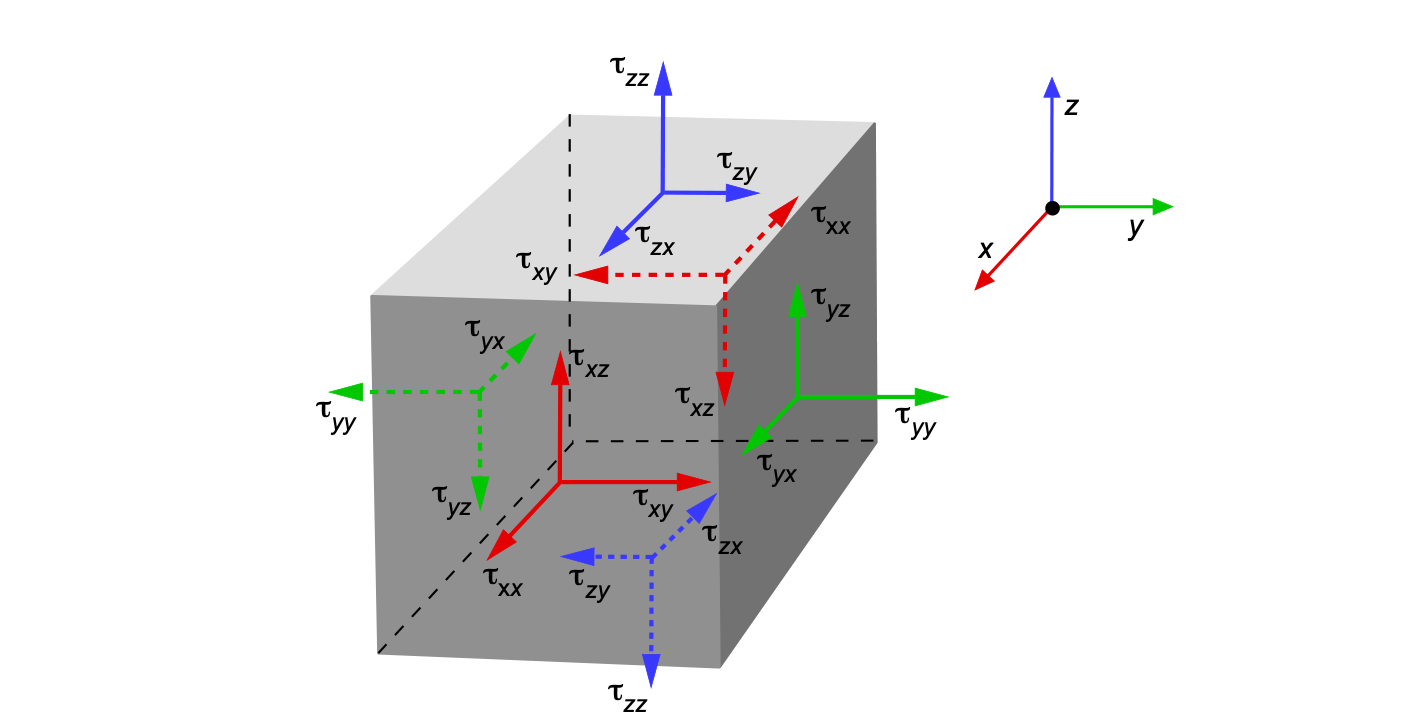
The indices i and j represent the coordinate directions , , and , where i denotes the plane on which the stress acts and j denotes the direction of the stress deformation. Notice that one normal stress component acts perpendicular to each face, and two shear stress components act tangentially to the face. For example, on the face perpendicular to the -direction, there is a normal stress,  , and the two shear stresses,
  and
and  . The normal stresses, ,
  , and
, and  , are often denoted as
  , and .
Viscous Forces
The net viscous force on the fluid in the direction is
(65) 
thereby giving
(66) 
The two other stresses in the direction are and  , as shown in the figure below. Therefore, the total viscous force contribution in the direction is
(67) 
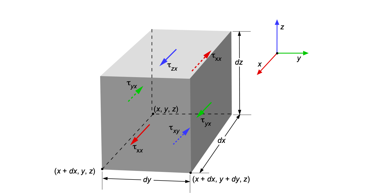 direction.
The stresses , , and  contribute to the force in the -direction, i.e., in aggregate they are
(68) 
Finally, the three remaining viscous shear stresses contribute to the force in the direction, i.e.,
(69) 
Collecting all of the contributions of the viscous stresses gives
(70) ![\begin{equation*} \vec{F}_{\mu} = \left\{ \begin{aligned} F_{x,\mu} & = \left( \frac{\partial \tau_{xx}}{\partial x} + \frac{\partial \tau_{yx}}{\partial y} + \frac{\partial \tau_{zx}}{\partial z} \right) d\mathcal{V}\\[6pt] F_{y,\mu} & = \left( \frac{\partial \tau_{yx}}{\partial x} + \frac{\partial \tau_{yy}}{\partial y} + \frac{\partial \tau_{zy}}{\partial z} \right) d \mathcal{V}\\[6pt] F_{z,\mu} & = \left( \frac{\partial \tau_{zx}}{\partial x} + \frac{\partial \tau_{zy}}{\partial y} + \frac{\partial \tau_{zz}}{\partial z} \right) d\mathcal{V} \end{aligned} \right. \end{equation*}](https://eaglepubs.erau.edu/app/uploads/quicklatex/quicklatex.com-e7d1e08034f625779be7054f5c70c98a_l3.svg "Rendered by QuickLaTeX.com")
Incorporating the stress terms into the momentum equations can be seen by first considering the -component, i.e.,
(71) 
and cancelling out the  term gives
(72) 
Similarly, for the -momentum equation, then
(73) 
and for the -momentum equation, then
(74) 
Therefore, combining the scalar components gives in vector form (which applies to a viscous laminar flow without body forces), then
(75) 
where the shear stress tensor is
(76) ![\begin{equation*} \vec{\tau} = \begin{bmatrix} \tau_{xx} & \tau_{xy} & \tau_{xz} \\[6pt] \tau_{yx} & \tau_{yy} & \tau_{yz} \\[6pt] \tau_{zx} & \tau_{zy} & \tau_{zz} \end{bmatrix} \end{equation*}](https://eaglepubs.erau.edu/app/uploads/quicklatex/quicklatex.com-c8aff26ea553435188e50d35557f165e_l3.svg "Rendered by QuickLaTeX.com")
With the body forces included, then
(77) 
Evaluating the Shear Stresses
Newton’s law of viscosity states that the shear stress is proportional to the rate of deformation (strain rate) of the fluid. Therefore, for a fluid with constant viscosity  , this relationship is written as
(78) 
In a flow where the velocity components are  in the -direction and
  in the -direction, the fluid’s deformation rate is determined by how the velocity changes in space. The strain rates for a fluid include terms that describe both normal (bulk) stresses and shear stress deformations. For the
  component of the shear stress, the strain rate is given by
(79) 
where the  term represents the rate at which the horizontal velocity changes with respect to the vertical coordinate , which contributes to shear. The
  term represents the rate at which the vertical velocity changes with respect to the horizontal coordinate , contributing to shear. The reason the strain rate has the sum of these two terms is because of the symmetry of the stress tensor, i.e., the stress (shear in the -plane) equals
  (shear in the
  -plane). Therefore, both velocity gradients and contribute to the shear stress. Therefore, the component is given by
(80) 
For the -component, then
(81) 
The momentum equation for the -component is given by
(82) 
where  are the components of the viscous stress tensor in the -direction. Substituting the expressions for , , and
(83) 
Simplifying gives
(84) 
This result can be written as
(85) 
where  is the Laplace operator. Similarly, for the -component, then
(86) 
Therefore, the -component of the momentum equation can be written as
(87) 
Finally, for the -component, then
(88) 
Therefore, the -component of the momentum equation can be written as
(89) 
Collecting all the viscous terms together, then
(90) ![\begin{eqnarray*} \varrho \frac{Du}{Dt} & = & -\frac{\partial p}{\partial x} + \mu \left( \frac{\partial^2 u}{\partial x^2} + \frac{\partial^2 u}{\partial y^2} + \frac{\partial^2 u}{\partial z^2} \right) = -\frac{\partial p}{\partial x} + \mu \nabla^2 u \\[8pt] \varrho \frac{Dv}{Dt} & = & -\frac{\partial p}{\partial y} + \mu \left( \frac{\partial^2 v}{\partial x^2} + \frac{\partial^2 v}{\partial y^2} + \frac{\partial^2 v}{\partial z^2} \right) = -\frac{\partial p}{\partial y} + \mu \nabla^2 v \\[8pt] \varrho \frac{Dw}{Dt}& = & -\frac{\partial p}{\partial z} + \mu \left( \frac{\partial^2 w}{\partial x^2} + \frac{\partial^2 w}{\partial y^2} + \frac{\partial^2 w}{\partial z^2} \right) = -\frac{\partial p}{\partial z} + \mu \nabla^2 w \end{eqnarray*}](https://eaglepubs.erau.edu/app/uploads/quicklatex/quicklatex.com-7cf5da72d790364729b4c31201b56e84_l3.svg "Rendered by QuickLaTeX.com")
In this case, these are referred to as the Navier-Stokes (N-S) equations in their incompressible, laminar form. In vector form, the N-S equations are
(91) 
With the body forces including gravity, the equation becomes
(92) 
The N-S equations (no body forces) can also be written in the form
(93) 
where  is the kinematic viscosity. Finally, in their most elegant form, the incompressible N-S equations are written as
(94) 
The Navier-Stokes equations are the most famous in fluid dynamics. These equations, a statement of Newton’s second law for a fluid, are fundamental to understanding fluid behavior. Despite their apparent simplicity, the N-S equations represent a set of coupled nonlinear partial differential equations, so solving them poses a significant challenge.[2] The N-S equations remain the cornerstone for studying fluid dynamics.
Summary & Closure
The principle of conservation of momentum is a cornerstone in fluid dynamics, and its use is necessitated whenever forces act on a fluid. The underlying principle is Newton’s second law of motion and is mathematically represented through the formal derivation of the momentum equation. This fundamental equation accounts for various forces that influence fluid motion, including body forces, pressure forces, and viscous forces. The momentum and continuity equations form the basis for analyzing and solving fluid flow problems. Depending on the specific situation, the momentum equation can be simplified by making appropriate assumptions, such as steady, inviscid, or incompressible flow. However, these simplifications must be carefully justified based on the physical context of the flow. In scenarios where pressure and temperature play a significant role, it becomes imperative to incorporate energy conservation principles to fully describe fluid behavior. This comprehensive approach ensures that all relevant forces and interactions are considered, resulting in a more accurate and thorough understanding of fluid flow dynamics.
The challenges of solving the Navier-Stokes equations extend well beyond their mathematical form because engineers must apply them to real-world scenarios. The Navier-Stokes equations are frequently employed to model turbulent flows, but predicting turbulence is also inherently problematic. Engineers now employ computational fluid dynamics (CFD) methods to find approximate numerical solutions to the Navier-Stokes equations and gain insights into the development of turbulent flows around flight vehicles. The Euler equations are often used as an initial approximation in computational fluid dynamics (CFD) simulations.
For Further Thought or Discussion
- Consider the flow through a reducing pipe with a 180
 bend. Show how to set up the equations to calculate the force of the fluid on the bend.
 - If the value of a force calculated using the momentum equation is negative, then what does this mean?
- Consider some flow problems where viscous effects are dominant, and an inviscid assumption for modeling the flow would likely be invalid.
- How might the momentum equation have to be modified to analyze turbulent flow?
- How might non-Newtonian fluids be treated differently in the momentum equation than Newtonian fluids?
Additional Online Resources
To learn more about the conservation of momentum applied to flow problems, check out some of these additional online resources:
- See an excellent, detailed explanation of the momentum equation in this video.
- A video explaining how to find the force from a flow through a nozzle.
- A (long!) video by an instructor explaining the conservation of momentum.
- MIT OpenCourseWare: Fluid Mechanics. Free course materials, including lecture notes, assignments, and exams from MIT’s course on advanced fluid mechanics.
- Coursera: Fluid Mechanics Courses. Universities worldwide offer various courses covering fundamental and advanced topics in fluid mechanics.
- YouTube: NPTEL Lectures on Fluid Mechanics. Comprehensive lecture series from India’s National Programme on Technology Enhanced Learning (NPTEL), covering fluid mechanics in detail.
- Wikipedia: Navier-Stokes Equations. An overview of the Navier-Stokes equations, their derivation, and applications in fluid dynamics.
- HyperPhysics: Fluid Dynamics. A comprehensive resource for physics concepts, including fluid dynamics and the application of the conservation of momentum.
- Journal of Fluid Mechanics. A leading journal that publishes high-quality research papers on all aspects of fluid mechanics.
- Physics of Fluids. An influential journal offering articles on fluid dynamics, including experimental, theoretical, and computational studies.
- SimScale: CFD Simulations. An online platform for computational fluid dynamics (CFD) simulations, providing practical applications of the conservation of momentum in fluid flow problems.
- PhET Interactive Simulations: Fluid Mechanics. Interactive simulations for visualizing and understanding concepts in fluid mechanics.
