Flight Vehicle Noise

J. Gordon Leishman

50 Flight Vehicle Noise

Introduction

Acoustics is the name given to the scientific study of sound generation, propagation, and reception. Noise is any unwanted or undesirable sound heard by a person, called an observer in acoustics terminology. The intensity, frequency, and duration of a sound can affect how an observer interprets the sound as being pleasant, acceptable, or “noisy.” By most standards, aircraft are considered by the general public as being noisy. Indeed, there have been concerns about aircraft noise since the earliest days of aviation. Most airplanes and airliners used before 1950 had no engine mufflers, and they used propellers that rotated at high tip speeds, generating a lot of noise. The critical engineering issues at that time were maximizing engine power and aircraft performance, and the resulting high noise levels were an inevitable byproduct. The public at large, however, viewed aircraft operations in the vicinity of airports as perpetually annoying, disrupting their work and home lives.

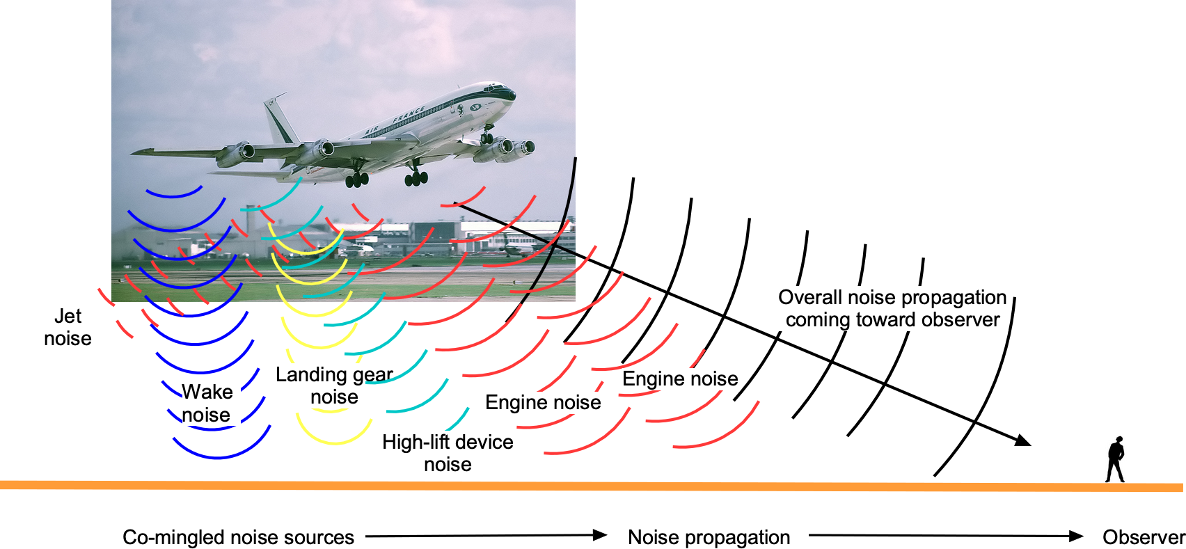
The 1950s saw the retirement of most airliners and military airplanes using piston engines and the adoption of turboprops and turbojets for propulsion. While more efficient and powerful, turbojet engines produced even higher noise levels, especially with jet airliners during takeoffs and landings. The loud “roar” and “whine” from turbojets resulted in a significant public backlash and legislative actions. Besides the dominant jet exhaust noise, airframe noise became more of a concern for these larger aircraft, as illustrated in the figure below. This latter type of noise, often described as “rumbling” and “swishing,” is generated by the movement of the airplane through the air.

An airplane creates several co-mingled noise sources from the engines and airframe.

Military aircraft can generate even greater noise levels because they use high-performance turbojet engines often augmented by afterburners. A lot of the noise from turbofan engines comes from the fan, which is of lower frequency but higher than that of a propeller; this engine type is much quieter overall than a turbojet. Rotorcraft, such as helicopters, tend to be noisy to observers because the noise frequencies produced by the rotor and tail rotor occur over the range that the human ear is sensitive to.

Pursuing approaches for noise reduction has become an increasingly significant consideration in aircraft design, especially as air travel has grown globally and more people are affected by aircraft noise. Noise regulations continue to become more stringent, and some airports may limit the operational time slots for noisier “legacy” jet aircraft. Internal noise is heard inside the aircraft, affecting the comfort and well-being of passengers, pilots, and crew. Advances in low-noise turbofan engines and acoustic absorption materials mean that airliners are much quieter inside the cabin than even a generation before, leading to increased comfort for passengers, especially on long-haul flights.

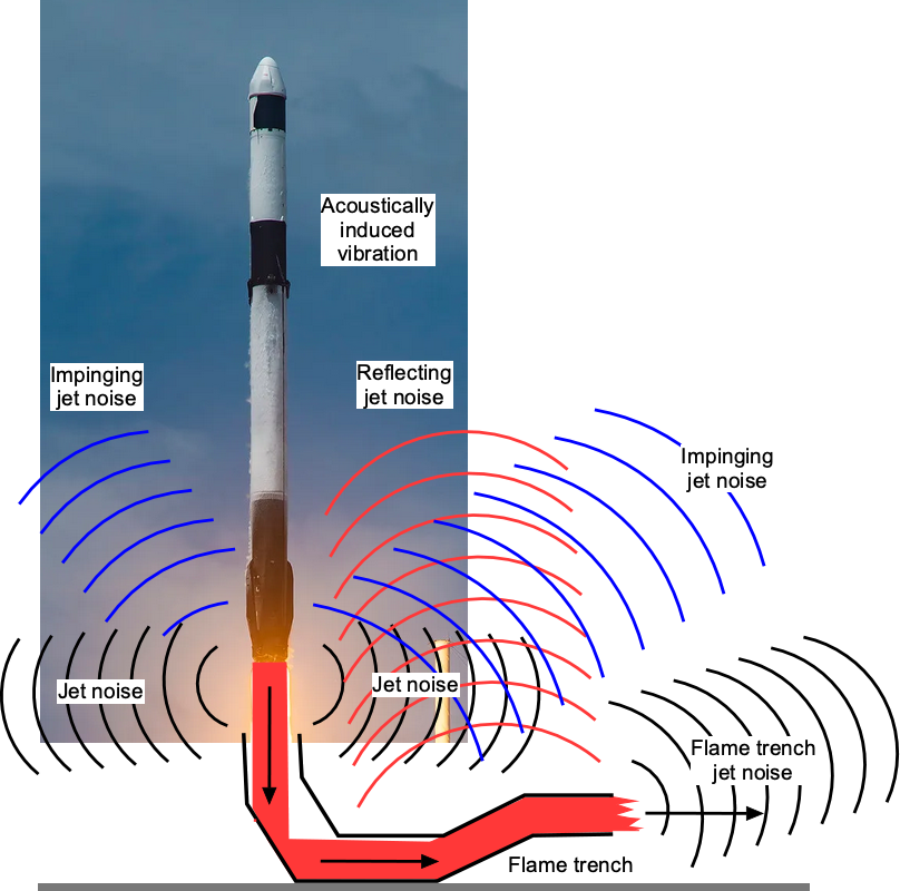
The space industry is not immune to noise concerns. Rocket noise, often called launch noise, is generated at different intensities and directions during the various phases of the launch profile, as shown in the figure below when the vehicle leaves the pad. Rocket motors generate an intense “crackling” noise from combustion and turbulent mixing in the supersonic exhaust (jet) flow, which will likely be above the threshold of pain for any observer within several miles of the launch point. This jet noise is also directional, i.e., mostly propagated in one dominant direction.

A rocket launch will produce intense noise levels from the high-speed gases exhausted from the rocket engines.

Learning Objectives

Be aware of aircraft noise sources, including engine and airframe noise.
Learn about the principles of acoustics and noise measurement.
Know the different noise metrics that can be used to assess the impact of aircraft noise.
Become familiar with the standards and regulations that apply to aircraft noise.
Appreciate the various impacts of aircraft noise and how it can be mitigated.

History of Aircraft Noise

Aircraft noise has been of concern since the earliest days of aviation. Even by the 1920s, aircraft use had become more widespread, and their noise levels had increased from using more powerful engines. Looking back, the first generation of piston-engine propeller-driven airplanes produced relatively mild noise levels compared to later jet engines. However, even these early aircraft, especially the larger aircraft such as the four-engined Lockheed Constellation and Douglas DC-7, produced significant “roar” and low-frequency “rumble,” mainly from their unmuffled exhaust systems. Their bigger propellers also increased the noise by adding higher-frequency impulsive noise, which sounds very “harsh” to an observer.

The introduction of jet engines in the 1950s was a quantum leap in aviation technology. While significantly increasing the speed and efficiency of aircraft, jet engines also produced substantially higher noise levels. The first type of “jet” airliners were turboprops, such as the Lockheed Electra and Vickers Viscount. Propeller-driven airplanes generate noise at relatively low frequencies, especially from multi-engine turboprops driving large propellers. Besides propeller noise, turboshaft engines driving propellers can produce a medium-frequency “shrill” that many observers find objectionable.

The noise generated by early jetliners with four turbojet engines, like the Boeing 707 and Douglas DC-8 in the late 1950s, quickly became of concern. These larger and faster aircraft also increased the number of passengers who wanted to fly, the upshot being an increase in the number of takeoffs and landings at major airports, much to the chagrin of those living or working nearby. Residents near airports and military bases began to seek relief from excessive aircraft noise, challenging expansion plans, capacity growth, and operating hours. Eventually, hush-kits had to be installed on the early jetliners, the most common type being a multi-lobe exhaust mixer.

Over the last few decades, continuing awareness of the environmental impact of aviation, including its noise levels, has led to widespread public concerns and regulatory actions. In response, governments and international organizations such as the International Civil Aviation Organization (ICAO) have started implementing increasingly stringent noise standards. These have included noise abatement procedures, restrictions on operating certain “historically noisy” aircraft types, and building new airports further away from populated areas. Aircraft manufacturers invested heavily in research and development to create quieter engines and airframes. Over the last decades, advancements such as high-bypass turbofan engines, improved aerodynamics, and noise mitigation technologies have significantly reduced aircraft noise.

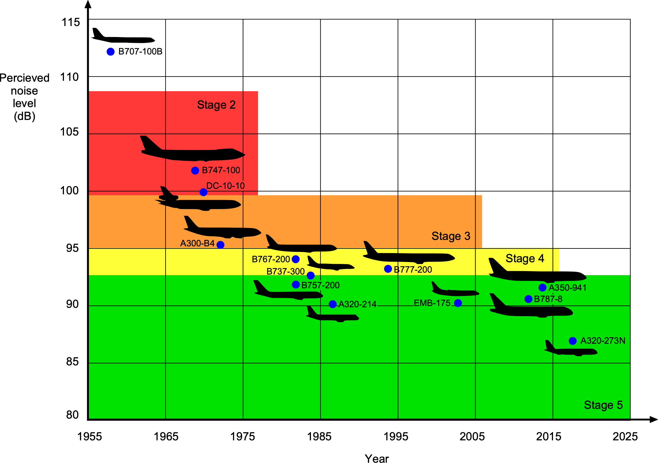
In the 1990s, the ICAO introduced the so-called “Balanced Approach” to noise mitigation. To this end, aircraft noise concerns were addressed through technological, operational, and planning measures. The approach also emphasized stronger collaboration between aircraft manufacturers, governments, and local communities. ICAO then established noise standards for aircraft, known as “Stages,” to categorize and regulate the noise emissions of different aircraft. Stage 3 noise standards were introduced in the 1970s, followed by Stage 4 standards in the 2000s, which set increasingly stricter limits on noise emissions for newly certified aircraft. Stage 5 is the current standard. As shown in the figure below, the noise levels of modern airliners are significantly quieter than those of even a generation ago, mainly because of the use of turbofan engines.

The noise levels of modern airliners have to meet much more stringent noise requirements, with many already meeting ICAO Stage 5 requirements.

During the 1900s, airframe and engine manufacturers continued to invest in research to develop technologies to reduce further noise emissions, with encouraging outcomes. In general, the pursuit of quieter aircraft remains a high priority for engine manufacturers, in particular, and the aviation industry as a whole. For example, the European Clean Sky program aims to develop cleaner air transport technologies, demonstrating and validating technologies capable of reducing greenhouse gasses and noise emissions “by 20% to 30% compared to state-of-the-art aircraft entering into service as from 2014.”

Research and development efforts continue on several fronts; the result is that newer aircraft generations have become increasingly quieter through sedulous engineering design to meet increasingly stringent noise standards, with many now reaching ICAO Stage 5 levels. Of interest to engineers is that EASA maintains a database of measured noise levels for all certified aircraft, including various airframe and engine combinations, as well as helicopters and general aviation types, that can be used for research and other purposes.

Introduction to Acoustics

Acoustics is the scientific study of sound, encompassing sound’s generation, transmission, and reception. In particular, aeroacoustics studies sound generation from aerodynamic forces, primarily those generated by lifting surfaces, and the propagation of this sound to an observer location. Sound can be described as a pressure disturbance or fluctuation in pressure that propagates as a wave through a given medium, usually air. This disturbance creates variations in the local air pressure, leading to the perception of sound by the ear. The knowledge gained by studying aeroacoustics and developing predictive computer noise models can be applied in engineering design to predict noise and help quieten aircraft.

Sound Waves

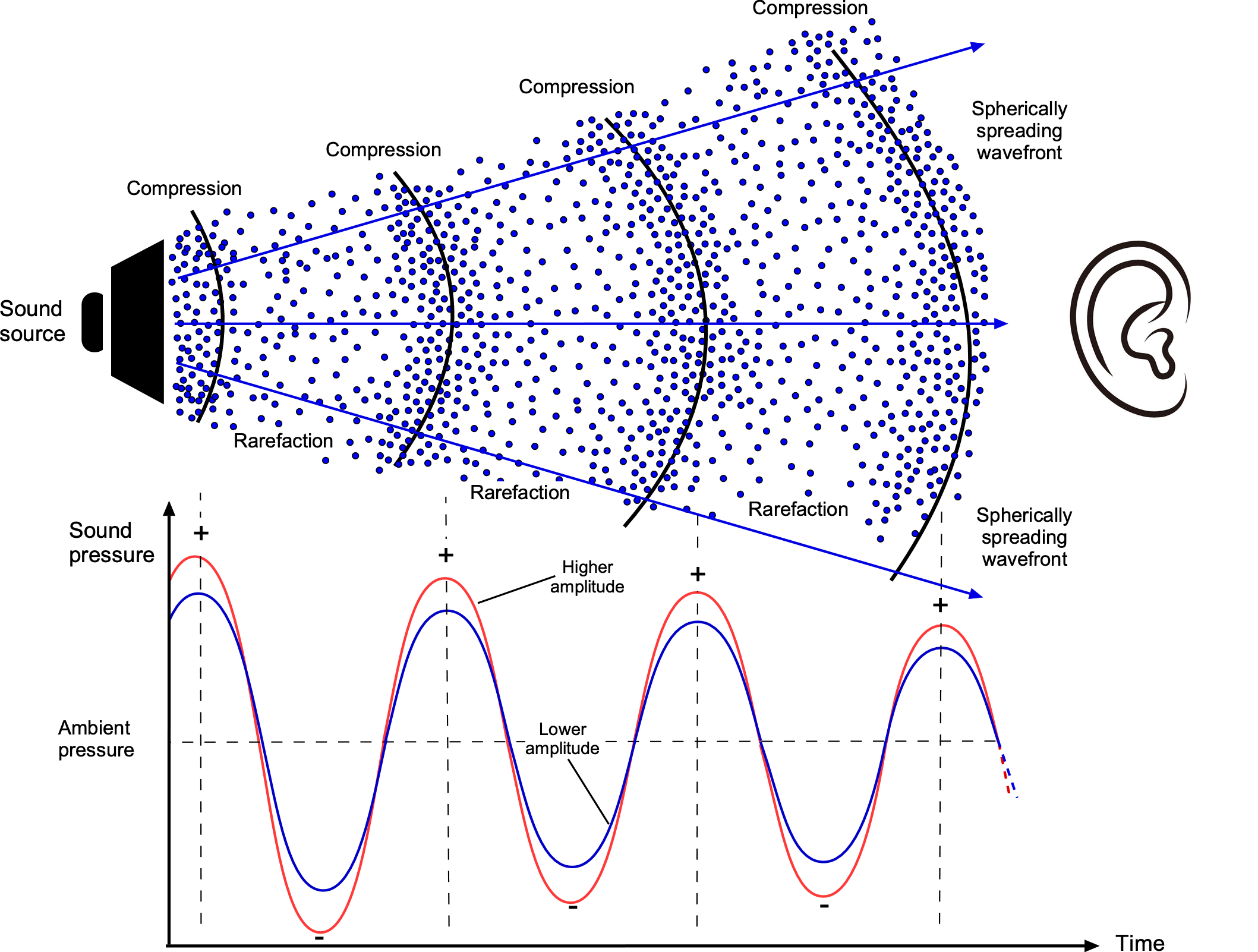
Sound is an energy wave that travels through the air by compressing and rarefying the molecules, as shown in the figure below. During compression, the air particles are pushed closer together or compressed, increasing pressure, as shown in the figure below. In a rarefaction, the particles move farther apart, resulting in a decrease in air pressure. Pressure is what the human ear responds to.

Sound is an energy wave that travels by compressing and rarefying the air molecules.

At any point along the path of wave propagation, the acoustic energy is stored in the medium through which the wave moves. The acoustic wave disrupts the molecular equilibrium and leads to a redistribution of molecular energy. For most common gases, including air, the molecular movement and relaxation are almost instantaneous to a passing sound wave. Therefore, energy is conserved to a good first approximation as the sound propagates through the air. However, in practice, molecular relaxation and viscosity effects absorb some acoustic energy in the atmosphere.

The amplitude of the pressure disturbance corresponds to the intensity or loudness of the noise an observer hears. Higher amplitude waves produce louder sounds, while lower amplitudes produce softer sounds. An observer interprets the frequency of a sound wave as its “pitch.” In this regard, the frequency of sound refers to the number of wave fronts arriving at the observer location per unit of time. Higher frequencies correspond to higher-pitched sounds, while lower frequencies result in lower-pitched sounds.

Compactness

When a body is large compared to the wavelength of the sound waves it generates, interference of wavefronts from different parts of the body produces complicated sound patterns. This behavior is especially important in the region near the body’s so-called near field. When the body is small relative to the wavelength scale of the sound it generates, or the sound is at high frequency, the phase differences between different source points are minor, and the body radiates sound energy like a point source. In acoustics, this relative size of the body at a given frequency is called its compactness, which is sometimes referred to as the compact source limit, as shown in the figure below. Therefore, a compact source radiates sound like a point source, whereas non-compact bodies in the near field must be treated in more detail.

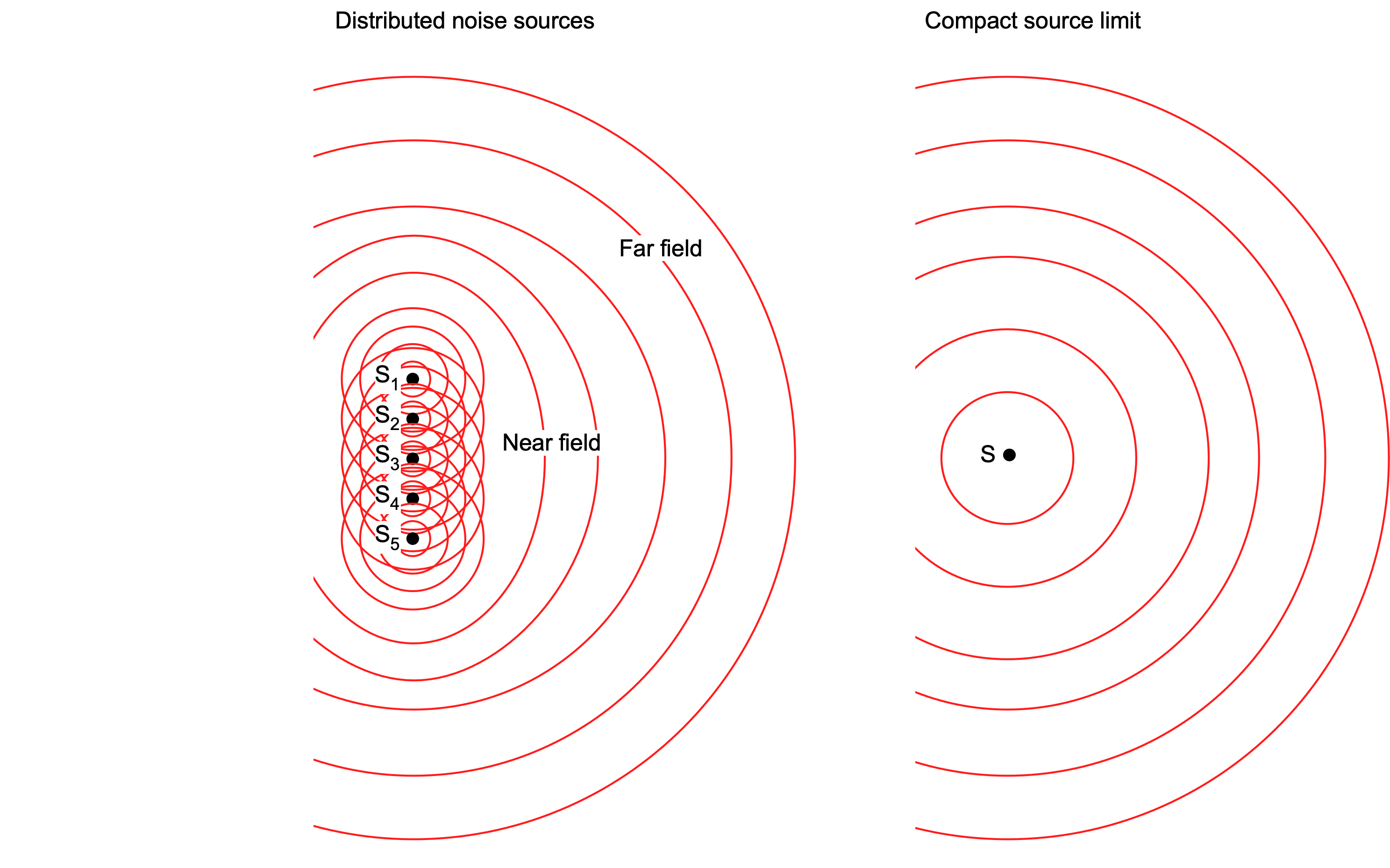
In the far field, distributed sound sources behave like a compact source.

The basic principle behind the compact source limit is that when the dimensions of the sound source are much smaller than the wavelength of the emitted sound, the source can be considered as a point or compact source. In this case, the sound waves radiate uniformly in all directions from the source, and the wavefronts are spherical. The compact source limit, therefore, allows for a simpler analysis compared to considering the detailed geometry of the acoustic sources.

Spherical Spreading

A sound disturbance from a compact or point source containing a specific sound power, $W$ , produces a spherical pressure wavefront that spreads out in time as it propagates away from the location of the original disturbance, which is called spherical spreading. Traditionally, in acoustics terminology, the sound power is given the symbol $W$ , but not to be confused with the units of power, a Watt (W). An assumption here is that the spreading occurs in a free field, which means no bounds or obstacles could affect the propagation. Sound power is the acoustic energy emitted per unit time and the rate at which the wavefront transfers sound energy.

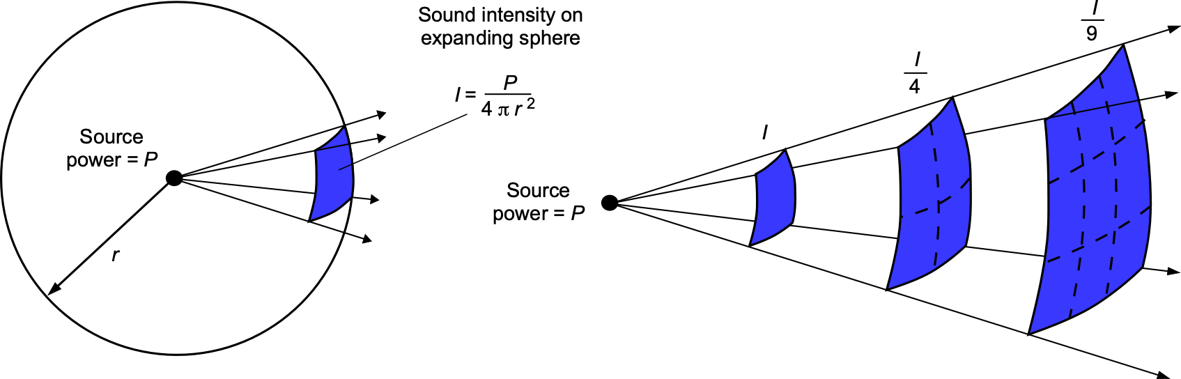
The intensity of the sound wave, $I$ , is the sound power divided by the perpendicular area over which this power is spread, i.e.,

(1) $\begin{equation*} I = \frac{W}{A} \end{equation*}$

If the spherical pressure wave has a radius, $r$ , the original power of the wavefront is now spread out over a spherical surface of area, $A = 4 \pi r^2$ . Therefore, the sound intensity, which is the power per unit area of an expanding spherical pressure wave, decreases inversely with the square of the distance, i.e., according to

(2) $\begin{equation*} I = \frac{W}{4 \pi r^2} \end{equation*}$

This result is called the inverse square law of sound, as illustrated in the figure below. Notice that sound intensity is a scalar quantity, just like pressure.

A sound disturbance produces a pressure wavefront that spreads spherically in time as it propagates away from the original disturbance.

The sound pressure of a traveling wave is proportional to the square root of its energy per unit area. The relationship between pressure and intensity is

(3) $\begin{equation*} p = \sqrt{ \frac{I}{Z}} = \sqrt{ \frac{I}{\varrho \, a}} \end{equation*}$

where $Z$ is called the impedance and measures how much the medium resists the transmission of sound waves.

The acoustic impedance depends on the density $\varrho$ and speed of sound $a$ in the medium as given by $Z = \varrho \, a$ . Therefore, substituting Eq. 2 into Eq. 3 gives

(4) $\begin{equation*} p = \sqrt{ \frac{W}{4 \pi \varrho \, a \, r^2} } = \sqrt{ \frac{W}{4 \pi \varrho \, a \, r^2} } \left( \frac{1}{r} \right) \, \propto \, \frac{1}{r} \end{equation*}$

Therefore, for a spherically traveling sound wave from a point source, the sound pressure will be proportional to $1/r$ , i.e., the pressure decreases inversely with distance. It can also be noted that sound power is proportional to the square of sound pressure, i.e., $W \, \propto \, p^2$ .

The sound pressure at point 2, a distance $r_2$ from the source, is related to the pressure at point 1, a distance $r_1$ from the source, by using

(5) $\begin{equation*} \frac{p_2}{p_1} = \frac{r_1}{r_2} \end{equation*}$

which follows the inverse distance law. Similarly, the sound intensities will be related by

(6) $\begin{equation*} \frac{I_2}{I_1} = \left( \frac{r_1}{r_2} \right)^2 \end{equation*}$

according to the inverse square law.

Multiple Sound Sources

As in most practical cases of acoustics, an aircraft is a complex noise source, with multiple interacting elements contributing to the noise field. These acoustic power sources will have different spatial locations and produce noise with various intensities and frequencies, which combine to give sound directivity to the net noise field, i.e., the directions of the flow of sound energy. The sound from any radiating body can be computed as the sum of spherical wave contributions from each source point on the body, i.e., as a superposition of spherical traveling waves. This basic principle is illustrated in the figure below, where the effects of the interfering sound waves from two separated source points can be seen to give regions of reinforcement and cancellation.

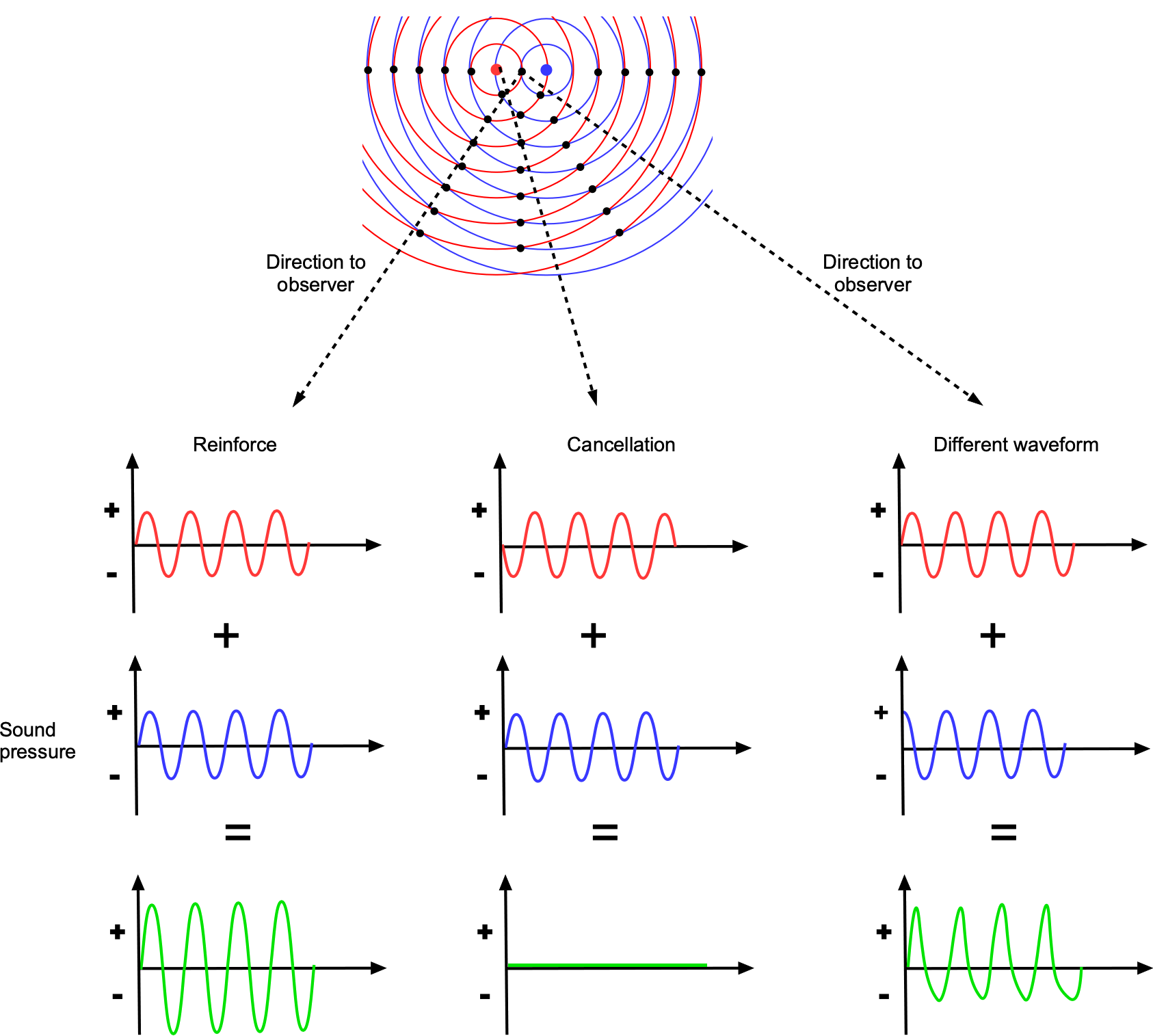
The net sound field from radiating bodies can be computed from a linear superposition of spherically traveling waves.

Therefore, different amplitudes and frequencies will be heard depending on where the observer is located in the sound field, i.e., there is a directivity pattern. Regions of wavefront reinforcement will give higher amplitude noise, i.e., acoustic hotspots, and regions of wave cancellation will result in reduced or no noise. Calculating the noise field for an actual aircraft is complicated, but the same fundamental principles apply. Simulations of this kind present numerous challenges because of the geometric complexities of aircraft and the high spatial and temporal resolution required to define the sound field.

Moving Sound Sources

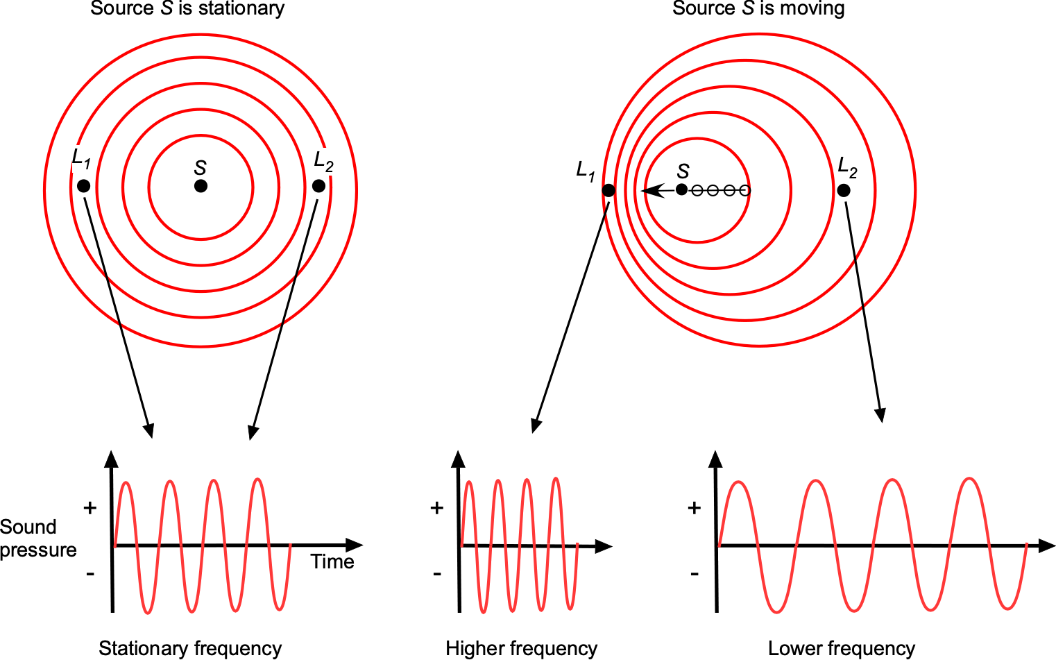
The task of predicting the sound field is complicated further by the fact that the sound sources originate at different times and are also moving with respect to an observer’s location. Sound is a pressure disturbance, and the speed of sound propagation in any gas at a given temperature will be constant. However, the perceived frequency of sound propagation will change if the location of the sound source S and the observer locations (say, L₁ and L₂) are in relative movement to each other, which is known as the Doppler effect, as illustrated in the figure below.

Illustration of the Doppler effect. — The perceived frequency of sound will depend on the relative velocity between the location of the sound source and the observer, i.e., a Doppler effect.

The frequency heard by an observer, $f_L$ , is given by

(7) $\begin{equation*} f_L = \left( \frac{a + V_L}{a + V_S} \right) f_S \end{equation*}$

where $V_S$ is the relative velocity of the source, $V_L$ is the relative velocity of the observer, and $f_S$ is the frequency of the sound source. The correct signs must be used on $V_S$ and $V_L$ ; the value of $V_S$ will be positive if the sound source moves away from the observer, and $V_L$ will be positive if the observer moves toward the source. In the figure above, the observer at $L_1$ will hear a higher frequency sound than at $L_2$ .

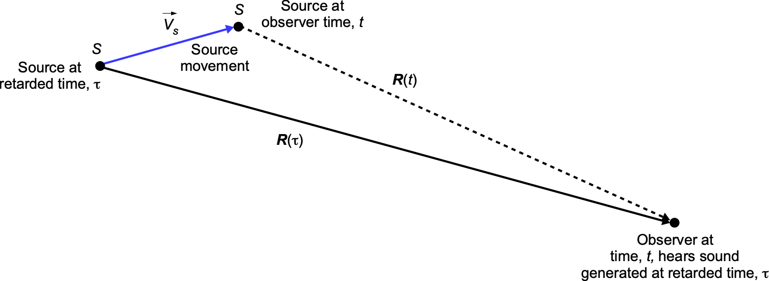
Retarded Time

As will now be apparent, a vital issue in any acoustic problem is determining the arrival time of sound waves at a given observer location in three-dimensional space. The evaluation of the resulting acoustic field requires accounting for either the time of emission of a sound wave from a source point, which in the case of an aircraft will be moving, relative to the current or observer time, i.e., a retarded time calculation. Alternatively, the arrival time of a sound wave relative to a given source time can be evaluated, i.e., an advanced time calculation.

Acoustic waves travel at the speed of sound plus or minus the local velocity of the fluid in which the waves propagate. This may be a nonuniform velocity field, which must be known a priori for the acoustics calculation. For example, in a stationary flow, the retarded time of the emission of a sound wave after it has traveled a distance $\bf{R}$ to reach the observer at time $t$ is given by

(8) $\begin{equation*} \tau = t^- = t - \frac{\bf{R}(\tau)}{a}, \end{equation*}$

or in a flow with velocity $v$ in the direction of $\bf{R}$ the retarded time is

(9) $\begin{equation*} \tau = t^- = t - \frac{\bf{R}(\tau)}{v+a}. \end{equation*}$

Therefore, the intensity of sound propagated by a moving acoustic source at any observer location must not be evaluated at the present time but according to what happened at a past or retarded time, as illustrated schematically in the figure below. This is a temporal mapping process and is fundamental to any acoustic calculation.

The intensity of sound propagated by a moving acoustic source to any observer location must be evaluated at a retarded time.

Alternatively, to avoid a retarded time calculation, the time of arrival of sound waves at the observer can be determined. This means that the future or advanced time of arrival of a wave at a given observer location is calculated using

(10) $\begin{equation*} t^+ = t + \frac{\bf{R}}{v+a}. \end{equation*}$

This approach means that all the acoustic waves must be tracked for a given source time, and the net sound field at a point in the acoustic field must be combined according to the arrival time. When using either the retarded time or advanced time formulation, the individual contributions from all wave sources from different source times are added together in amplitude and phase at each observer position and time.

Wave Tracing

These ideas of the source and arrival times of sound waves at observer locations are embodied in a process known as wave tracing. In a fixed reference frame with respect to the body, the wavefronts that propagate radially from each source point proceed at the local speed of sound plus the flow velocity component in the propagation direction. For example, for an outward-moving source point, the initial wavefront trajectory over a period $\Delta t$ can be formalized as

(11) $\begin{equation*} \vec{x} = \left\{ \begin{array}{c} x \\ y \\ z \end{array} \right\} = \left\{ \begin{array}{c} x_B \\ y_B \\ z_B \end{array} \right\} + \left[ \begin{array}{c} a t_s + u \\ a t_s + v \\ (a + w) \end{array} \right] \Delta t \end{equation*}$

where $(x_B, y_B, z_B)$ is the acoustic source point, $t_s$ of the acoustic source point, and $(u,v,w)$ can be considered as the local flow velocities relative to a defined coordinate system.

Consider an example of the sound field radiated by a rotating source with a subsonic Mach number. Assume that an acoustic source at a given radius rotates about a central point at frequency $\Omega$ . The figure below shows that the wavefronts coalesce along a spiral and move away from the source point at the speed of sound. These sound wave patterns are also similar to those produced on propellers, which are discussed later in this chapter.

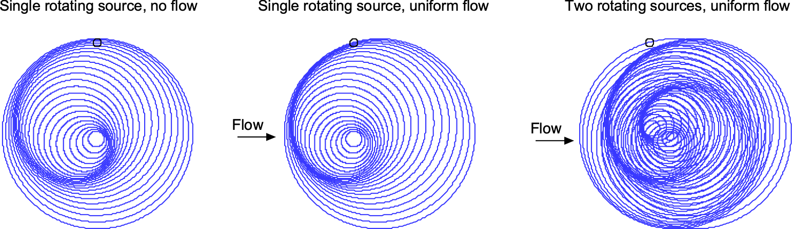
The propagating sound produced by a rotating source will coalesce along spiral wavefronts.

The addition of a flow speed, from left to right, shows that the wavefronts propagate at the speed of sound plus or minus the local flow velocity. It will be apparent that the upstream moving waves bunch closer together, and the downstream moving waves are spread further apart. As previously discussed, this is a Doppler effect, manifesting as an increase or decrease of the apparent sound frequency and intensity at upstream or downstream observer locations. Adding a second source makes the sound field somewhat more complicated, but the principles are the same.

Ffowcs Williams-Hawkings Equation

The movement of all the acoustic waves in the sound field is formally embodied in the Ffowcs Williams-Hawkings (FW-H) equation. This equation incorporates the fundamental principles of mass, momentum, and energy conservation as a wave equation. According to the F-WH equation, the acoustic pressure, $p$ , at a point $\vec{x}$ at time $t$ can be written in the form

(12) $\begin{eqnarray*} p(\vec{x},t) & = & \frac{1}{4\pi}\frac{\partial}{\partial t} \iint\limits_S \left[ \frac{\varrho v_n}{{\bf R} (1-M_{{\bf R}})}\right]_{\tau} dS + \frac{1}{4\pi a} \frac{\partial}{\partial t} \iint\limits_S \left[ \frac{l_{{\bf R}}}{{\bf R} (1-M_{{\bf R}})} \right]_{\tau} dS \nonumber \\ & & \quad \quad + \frac{1}{4\pi} \iint\limits_S \left[ \frac{l_{{\bf R}}}{{\bf R}^2 (1-M_{{\bf R}})} \right]_{\tau} dS \end{eqnarray*}$

where $l_{\bf R}$ is the total force on the fluid at each source point on a surface $S$ in the direction of the observer, and $\tau$ is the retarded time. The parameter $M_{{\bf R}}$ is the relative Mach number from the source point in the observer’s direction, accounting for the Doppler effect.

The first term in Eq. 12 is the thickness noise, which involves a determination of the perturbation velocity, $v_n$ , produced by the body as it passes through the flow. The second and third terms are the loading noise resulting from the body’s aerodynamic forces. The third term is a near-field sound term, which does not represent a propagating wave. Notice that the first part of the loading noise is related to the time rate of change of the pressure on a lifting surface.

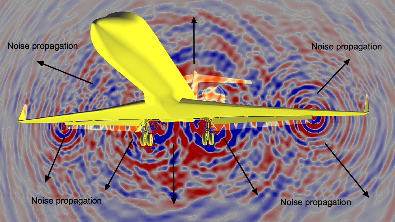
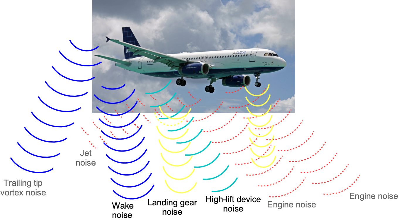
In practice, the FW-H equation is evaluated numerically, although it is mostly geometry and wave tracing, for which various computer codes are available. The most significant challenges in finding the acoustic field are describing the geometry of the body, which can be complex for an aircraft, and determining the aerodynamic loads. For example, the image below shows the plethora of sound waves generated from an airliner. The interacting wavefronts show the complexity of the sound field. Notice a concentration of sound waves from the engines (jet noise) and the vortices trailed from the outboard edges of the flaps (airframe noise). You can gain a deeper understanding of airframe noise by viewing this video.

The noise field produced by an aircraft is remarkably intricate, not least because of the complex geometry of the airframe.

Quantifying Sound Using Decibels

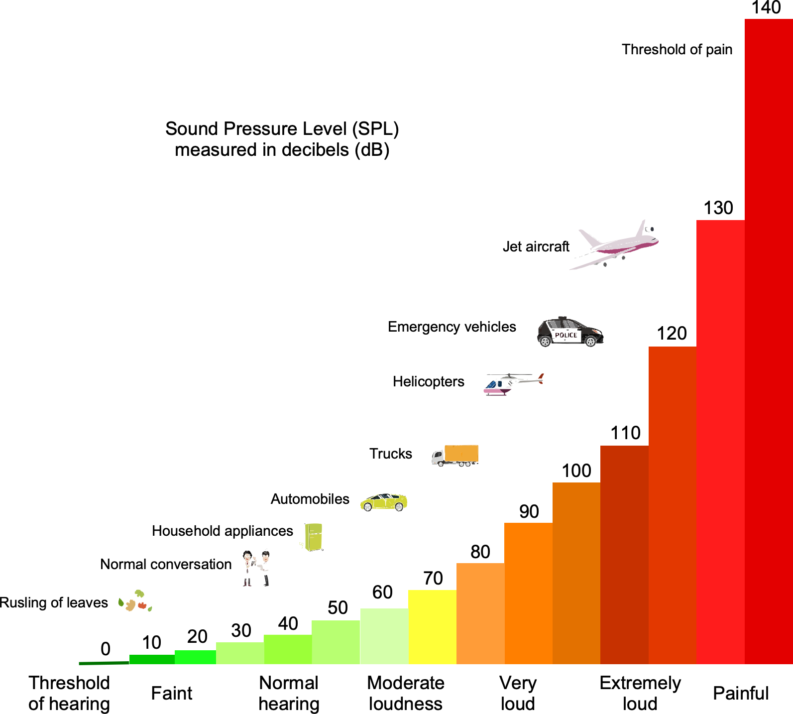
The intensity of sound and noise is quantified using the decibel (dB) scale, as illustrated in the figure below, which is a logarithmic scale. A logarithmic scale is used because it can be used to quantify the wide range of pressures that the human ear can perceive, from the faintest sound, such as the buzz of a bee, to the loudest sound that can be tolerated, such as an explosion or a gunshot. The variations in pressure between those two extremes are about six orders of magnitude.

The Bel (B) is the unit used to measure the ratio of sound power on a logarithmic scale. The sound power, $L_{W}$ , in units of Bel, is defined as

(13) $\begin{equation*} L_{W} = \log_{10} \left(\frac{W}{W_0} \right) \end{equation*}$

where $W_0$ is a reference power, which is $W_0 = 1.0 \times 10^{-12}$ Watt (W) or one pW (pica-Watt), considered as the sound power at the threshold of human hearing. Notice that the Bel is a dimensionless quantity. In terms of pressure, then

(14) $\begin{equation*} L_{W} = \log_{10} \left(\frac{p^2}{p_0^2} \right) = 2 \log_{10} \left(\frac{p}{p_0} \right) \end{equation*}$

where $p_0$ is the reference pressure, noting that $W \, \propto \, p^2$ . The reference pressure corresponding to the same hearing threshold is $p_0 = 20 \times 10^{-6}$ Pa = 20 $\mu$ Pa. To get better granularity in the numerical scale, the “deci-Bel” or decibel (dB) is used, which is just one-tenth of a Bel, so in terms of dB values, then

(15) $\begin{equation*} L_{W} = 20 \log_{10} \left(\frac{p}{p_0} \right) \end{equation*}$

Notice that the threshold of human hearing becomes 0 dB on the decibel scale. At the upper end of the decibel scale, the pain threshold is about 140 dB. The value of $L_W$ is often called the sound power level (SWL) or acoustic power level.

The corresponding relationship between the sound intensity level, $L_p$ (in dB), and intensity is

(16) $\begin{equation*} L_p = 10 \log_{10}\left(\frac{I}{I_0} \right) \end{equation*}$

where $I_0$ is the reference intensity defined as $I_0 = 1.0 \times 10^{-12}$ W m $^{-2}$ or 0.000000000001 W m $^{-2}$ , which is the threshold of hearing. The threshold of pain regarding sound intensity is about 1 W m $^{-2}$ . Because of the enormous range of intensities that the ear can perceive (12 decades), it now makes sense why the logarithmic scale is so convenient to use.

To better understand the meaning and use of the decibel scale, consider a change in sound intensity $\Delta I$ . The corresponding change in sound intensity level will be

(17) $\begin{equation*} \Delta L_p = 10 \log_{10}\left(\frac{\Delta I}{I_0} \right) \end{equation*}$

For example, if $\Delta I / I_0 = 2$ , which is a doubling of the sound intensity, then

(18) $\begin{equation*} \Delta L_p = 10 \log_{10} (2) = 3.0~\mbox{dB} \end{equation*}$

Therefore, each 3 dB increment means a doubling of sound intensity (which translates to a 6 dB increase in sound pressure), and each 3 dB decrement means a halving of sound intensity (or a 6 dB decrease in sound pressure).

Worked Example #1 – Sound intensities and decibels

What is the intensity of a 60 dB sound that produces a broadband white-noise source compared to a similar 50 dB source?

In this case, we need to rearrange the equation for $L_p$ , i.e.,

$L_p = 10 \log_{10}\left(\frac{I}{I_0} \right)$

to solve for $I$ . Using the principles of logarithms, then

$I = I_0 \, 10^{\frac{L_p}{10}}$

For the 50 dB source, then

$I_{50} = I_0 \, 10^{\frac{50}{10}} = 1.0 \times 10^{-7}~\mbox{W m$^{-2}$}$

Similarly, for the 60 dB source, then

$I_{60} = I_0 \, 10^{\frac{6}{10}} = 1.0 \times 10^{-6}~\mbox{W m$^{-2}$}$

Notice then that a 10 dB increase means the sound intensity has increased ten times.

Listen to the difference in what 10 dB makes to sound level here!

Sound Pressure Level (SPL)

The Sound Pressure Level (SPL) is the most fundamental metric for measuring sound intensity, including aircraft noise. SPL is commonly used in the same context as $L_W$ and $L_p$ because it refers to the same fundamental concepts but is a more specific term in practical applications. In many cases, engineers generally use SPL when discussing the measurement of sound or noise. The SPL is calculated using

(19) $\begin{equation*} \text{dB}_{\rm SPL} \equiv \text{SPL} = 20 \log_{10}\left(\frac{p_{\rm rms}}{p_0}\right) \end{equation*}$

where $p_{\rm rms}$ is the sound pressure’s root mean square (rms), and $p_0$ is the reference sound pressure. The root mean square value of the sound pressure is given by

(20) $\begin{equation*} p_{\rm rms} = \sqrt{ \frac{1}{(t_2 - t_1 )} \int_{t_1}^{t_2} p(t)^2 \, dt } \end{equation*}$

where $t_2 - t_1$ is the time interval over which the sound pressure is measured.

Notice that for a spherically spreading sound wave, the SPL values at two distances $r_1$ and $r_2$ will be related by

(21) $\begin{equation*} \text{SPL}_2 = \text{SPL}_1 -20 \log_{10} \left( \frac{r_2}{r_1} \right) \end{equation*}$

Therefore, if the distance is doubled such that $r_2$ = $2 r_1$ , then the change in SPL will be

(22) $\begin{equation*} \Delta \text{SPL}_2 = -20 \log_{10} (2) = 6.02~\mbox{dB} \end{equation*}$

This means the SPL decreases by about 6 dB for every doubling of the distance.

Worked Example #2 – Calculating SPL values at different distances

An observer at point O₁ at a distance $r_1$ = 3 m from a sound source measures an SPL of 72 dB. What will be the SPL at location 0₂at a distance $r_2$ = 8 m from the sound source? How far must the observer at location 0₂be from the sound source to measure an SPL of less than 58 dB? Assume spherical spreading.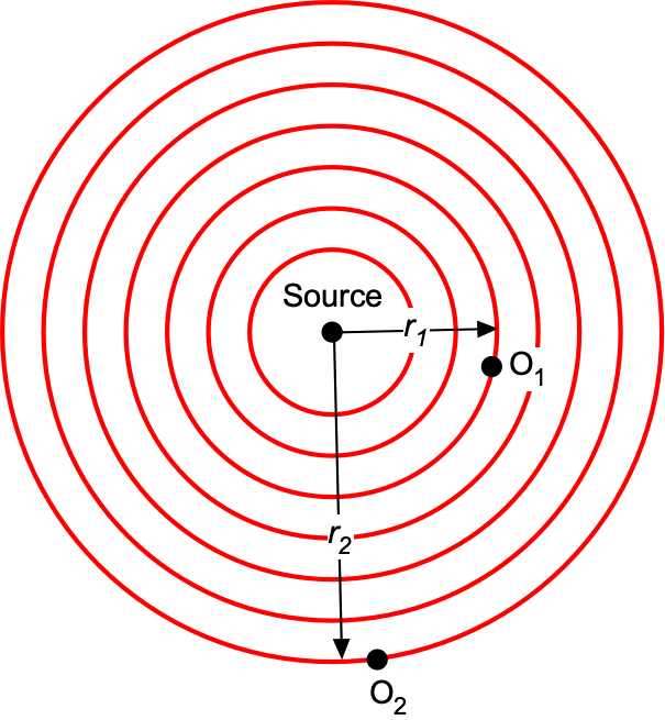

The values of the SPL will be related using the inverse distance law, i.e.,

$\text{SPL}_2 = \text{SPL}_1 -20 \log_{10} \left( \frac{r_2}{r_1} \right) = \text{SPL}_1 -20 \log_{10} \left( \frac{8}{3} \right) = 72.0 - 8.52 = 63.5~\mbox{dB}$

Therefore, the SPL at location 0₂will be 63.5 dB. If the observer now needs to move further away to obtain an SPL of less than 58 dB, then

$58.0~\mbox{dB} = \text{SPL}_2 = \text{SPL}_1 -20 \log_{10} \left( \frac{r_2}{r_1} \right) = 72.0 -20 \log_{10} \left( \frac{r_2}{3.0} \right)$

Taking antilogs gives

$r_2 = 3.0 \times 10^{ \frac{(72.0 - 58.0)}{20}} = 15.04~\mbox{m}$

Therefore, the distance needed to obtain an SPL of less than 58 dB will be at least 15 m.

Adding Sound Values

The sound levels cannot be added in decibels based on the logarithmic scale when adding sound pressure values from different sources. Therefore, the dB values must first be converted into pressure or intensity values, which can be added linearly.

Sound Pressure

Recall that in terms of pressure, then

(23) $\begin{equation*} \text{SPL} = 20 \log_{10}\left(\frac{p}{p_0}\right) \end{equation*}$

where the reference pressure is $p_0 = 20 \times 10^{-6}$ Pa. Using the principles of logarithms gives

(24) $\begin{equation*} p = p_0 \, 10^{\frac{SPL}{20}} \end{equation*}$

For $N$ sound sources with individual sound pressure values ${\rm db}_i$ , then

(25) $\begin{equation*} \text{SPL}_{\rm tot} = 20 \log_{10}\left(\frac{p_1 + p_2 + p_3 + ... p_n}{p_0}\right) \end{equation*}$

which becomes

(26) $\begin{equation*} \text{SPL}_{\rm tot} = 20 \log_{10} \left ( \frac{ p_0 \left( 10^{\frac{{\rm db}_1}{20}} + 10^{\frac{{\rm db}_2}{20}} + 10^{\frac{{\rm db}_3}{20}} + \cdots + 10^{\frac{{\rm db}_N}{20}} \right)}{p_0} \right) \end{equation*}$

With some further rearrangement, then

(27) $\begin{equation*} \text{SPL}_{\rm tot} = 20 \log_{10}\left( 10^{\frac{{\rm db}_1}{20}} + 10^{\frac{{\rm db}_2}{20}} + 10^{\frac{{\rm db}_3}{20}} + \cdots + 10^{\frac{{\rm db}_N}{20}} \right) \end{equation*}$

and finally,

(28) $\begin{equation*} \text{SPL}_{\rm tot} = 10 \log_{10}\left( 10^{\frac{{\rm db}_1}{10}} + 10^{\frac{{\rm db}_2}{10}} + 10^{\frac{{\rm db}_3}{10}} + \cdots + 10^{\frac{{\rm db}_N}{10}} \right) \end{equation*}$

noting that $10 \log_{10} \left(10^{{\rm db}/10} \right)$ is equal to $20 \log_{10} \left(10^{{\rm db}/20} \right)$ .

Sound Intensity

In terms of sound intensity, then

(29) $\begin{equation*} \text{SPL}_{\rm tot} = 10 \log_{10}\left( \frac{\left( I_1 + I_2 + I_3 + \cdots + I_N \right) }{I_0}\right) \end{equation*}$

where $I_0 = 1.0 \times 10^{-12}$ W m $^{-2}$ . Following the same approach as for the pressure, then

(30) $\begin{equation*} I = I_0 \, 10^{\frac{SPL}{10}} \end{equation*}$

so, for $N$ sound sources, then

(31) $\begin{equation*} \text{SPL}_{\rm tot} = 10 \log_{10}\left( \frac{I_0 \left( 10^{\frac{{\rm db}_1}{10}} + 10^{\frac{{\rm db}_2}{10}} + 10^{\frac{{\rm db}_3}{10}} + \cdots + 10^{\frac{{\rm db}_N}{10}} \right)} {I_0}\right) \end{equation*}$

With some further rearrangement, then

(32) $\begin{equation*} \text{SPL}_{\rm tot} = 10 \log_{10}\left( 10^{\frac{{\rm db}_1}{10}} + 10^{\frac{{\rm db}_2}{10}} + 10^{\frac{{\rm db}_3}{10}} + \cdots + 10^{\frac{{\rm db}_N}{10}} \right) \end{equation*}$

which is the same result as given previously in Eq. 28. Therefore, adding acoustic pressures is equivalent to adding acoustic intensities.

Worked Example #3 – Adding the effects of sound sources

Consider two separate sound sources producing white noise. An observer measures a sound pressure level of 80.0 dB from one source and 87.0 dB from the other. What is the resulting sound pressure level when both sources are active?

The dB values cannot be added, so it is necessary to convert the dB_1 and dB_2 values into intensities, $I_1$ and $I_2$ . For the first source, then

$I_1 = I_0 \, 10^{\frac{db_1}{10}} = 1.0 \times 10^{-12} \times 10^{\frac{80.0}{10}} = 1.0 \times 10^{-4}~\mbox{W m$^{-2}$}$

and for the second source, then

$I_2 = I_0 \, 10^{\frac{db_2}{10}} = 1.0 \times 10^{-12} \times 10^{\frac{87.0}{10}} = 5.01 \times 10^{-4}~\mbox{W m$^{-2}$}$

Therefore, the sum of the intensities is

$I_{\rm tot} = I_1 + I_2 = 1.0 \times 10^{-4} + 5.01 \times 10^{-4} = 6.01 \times 10^{-4}~\mbox{W m$^{-2}$}$

Converting back to dB values gives

$dB_{\rm tot} = 10 \log_{10} \left( \frac{I_{\rm tot}}{I_0} \right) = 10 \log_{10} \left( \frac{6.01\times 10^{-4}}{1.0 \times 10^{-12}} \right) = 87.8~\mbox{dB}$

Notice that the source producing sound at the lower level makes very little difference to the net sound, which is dominated by the second source.

Note: Try this problem again using pressures instead of intensities, and convince yourself that you get the same answer.

Human Hearing

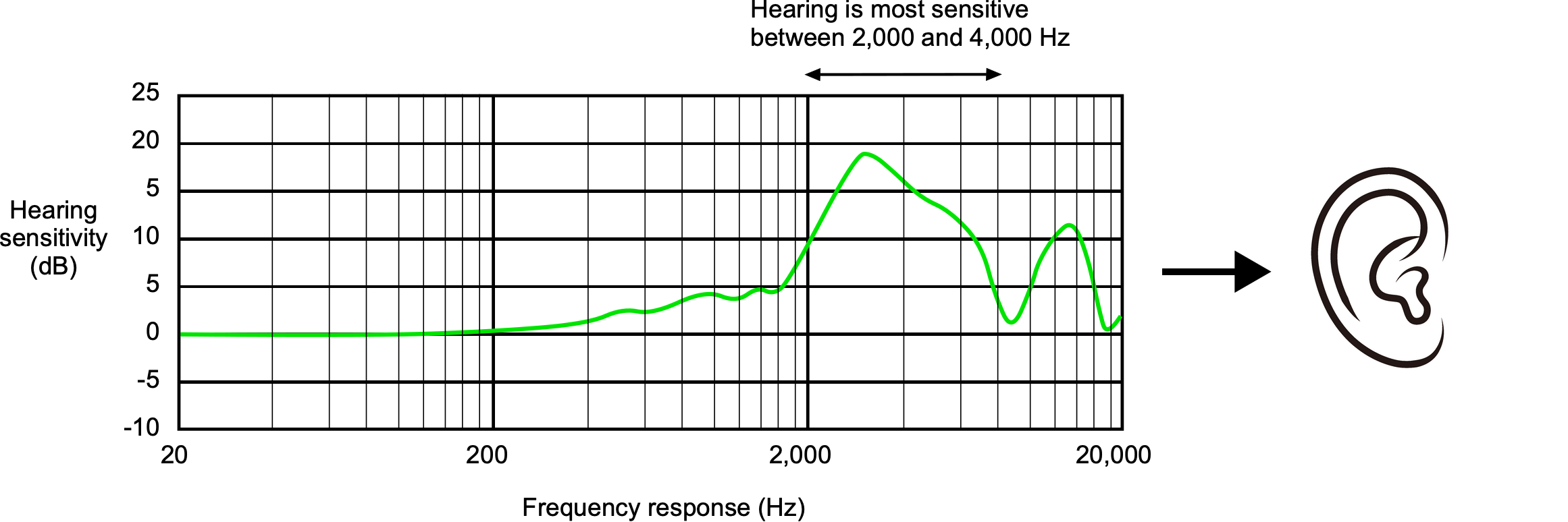
The ear’s anatomy enables the brain to perceive and interpret various sound qualities, including pitch (frequency) and loudness (intensity). However, the human ear has a nonlinear spectral sensitivity regarding frequency versus amplitude. For example, humans do not perceive low-frequencies (less than 100 Hz) or high-frequency sounds (more than 18,000 Hz). The ear is most sensitive to sounds between 1,000 Hz and 4,000 Hz, unsurprisingly the frequency range of human speech, as shown in the figure below, which is often expressed in terms of an equal-loudness contour.

The human ear’s frequency response is nonlinear and most sensitive to sounds between 1,000 and 4,000. Hz.

Because the frequency response of human hearing is nonlinear, psychoacoustic weightings have been established for measuring and comparing sound pressures. The A-weighted sound pressure is the most commonly used, given the symbol dB_A or dB(A), which is designed to mimic the human ear’s sensitivity to different frequencies that occur at lower sound levels. The weighting attenuates the contribution of low and high frequencies but emphasizes the midrange frequencies where human hearing is most sensitive.

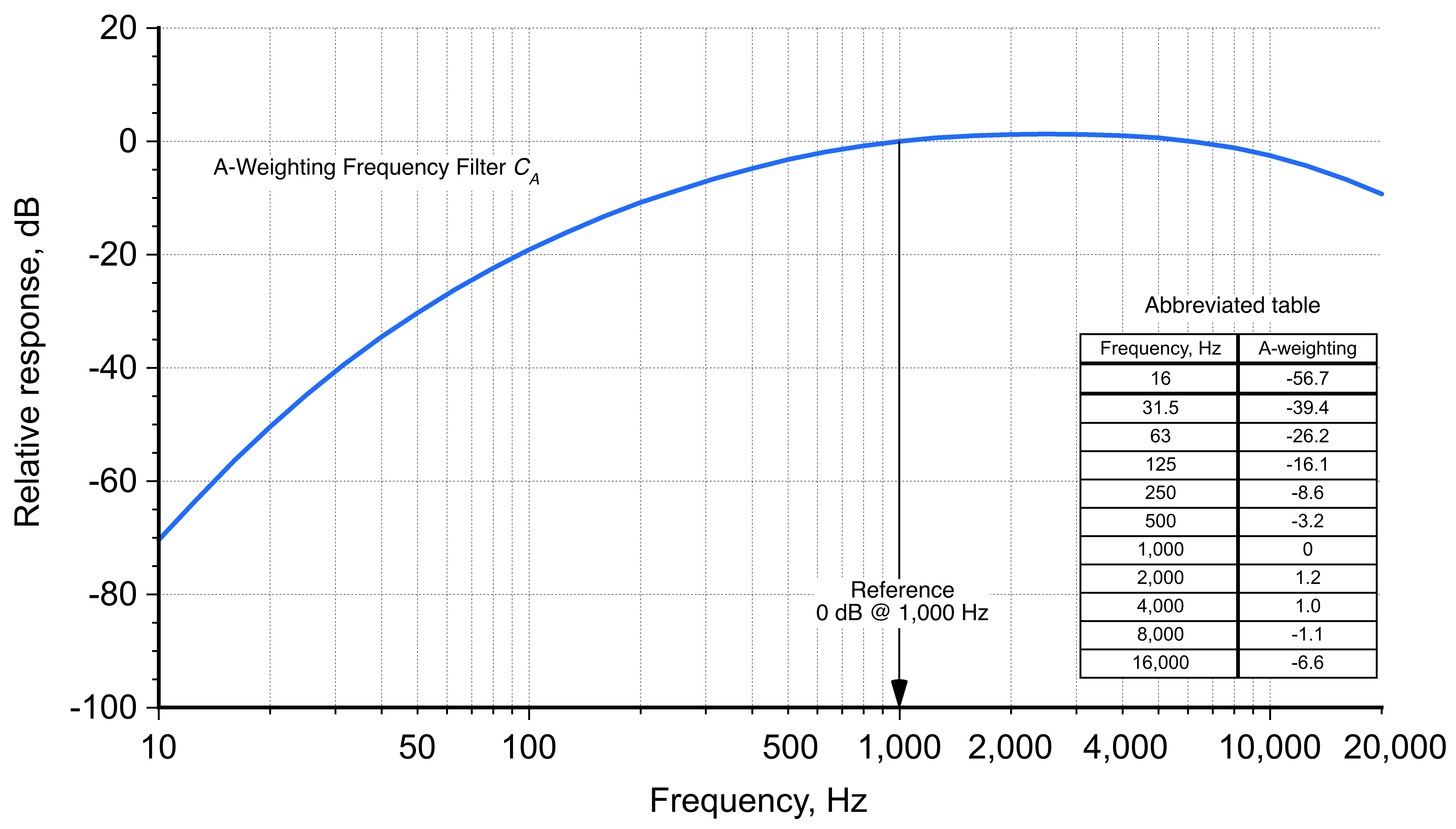
The A-weighted sound pressure dB(A) mimics the human ear’s frequency sensitivity.

The A-weighting filter can be represented by

(33) $\begin{equation*} \text{SPL}_A = \text{SPL} + C_A \end{equation*}$

where $\text{SPL}_{A}$ is the required A-weighted sound level in decibels, $\text{SPL}$ is the unweighted level at a given frequency, and $C_A$ is a frequency-dependent correction factor determined by the A-weighting curve, as shown above. The specific values of $C_A$ for different frequencies are defined by international standards, such as ISO 226:2023, but a MATLAB code is also available.

The equation used for calculating the overall A-weighted continuous sound level from measured sound levels at different frequencies is

(34) $\begin{equation*} \text{SPL}_A = 10 \cdot \log_{10} \left( \sum_{i=1}^{n} C_i \, 10^{\left(\frac{\text{SPL}_i}{10}\right)} \right) \end{equation*}$

where $\text{SPL}_A$ is the A-weighted equivalent continuous noise level, $\text{SPL}_i$ is the measured sound level at each frequency band, $C_i$ is the corresponding A-weighting filter value for each frequency band, and $N$ is the total number of frequency bands. The process can be programmed in MATLAB, as shown in the worked example below.

Worked Example #4 – Calculating A-weighted sound levels

Write a short piece of MATLAB code to calculate the A-weighted continuous SPL. To test the code, SPL values are given at eight discrete frequencies, which are 80 dB, 85 dB, 90 dB, 95 dB, 100 dB, 95 dB, 85 dB, and 80 dB, with the corresponding A-weights being -26.2 dB -16.1 dB, -8.6 dB, -3.2 dB, 0.0 dB, 1.2 dB, 1.0 dB, and -1.1 dB.

function SPLAeq = calculate_A_weighted_level(SPLs, A_weights)
% SPLs: A-weighted Sound Pressure Levels at different frequencies
% A_weights: A-weighting filter values for corresponding frequencies
% Ensure that the number of SPLs and A_weights match
SPLs = [80, 85, 90, 95, 100, 95, 85, 80];
% A-weighted SPLs in dB for each frequency band
A_weights = [-26.2, -16.1, -8.6, -3.2, 0.0, 1.2, 1.0, -1.1];
% A-weighting filter values
SPLAeq = calculate_A_weighted_level(SPLs, A_weights);
if length(SPLs) ~= length(A_weights)
error(‘Number of SPLs and A_weights must be the same.’);
end
% Calculate the A-weighted level using the formula
sum_terms = sum(10.^(SPLs / 20) .* 20.^(A_weights / 20));
PLAeq = 20 * log10(sum_terms);
end
fprintf(‘A-weighted equivalent continuous noise level: %.2f dB(A)\n’, SPLAeq);

Is it possible to have negative values of dB?

Yes! In an anechoic chamber, which is specifically designed to minimize reflections of sound waves, it is possible to measure sound pressure levels below the threshold of human hearing using a sensitive microphone. Recall that the SPL is given by

$\text{SPL} = 20 \log_{10}\left(\frac{p_{\rm rms}}{p_0}\right)$

So if the measured sound pressure, $p_{\rm rms}$ , is less than the reference sound pressure, $p_0$ , then the logarithm in this equation will be negative, resulting in a negative value of SPL. However, it should be appreciated that this result does not imply a negative sound pressure but rather a level below the threshold of normal human hearing.

Noise = Unwanted Sound

Many sounds are pleasant, e.g., music, ocean waves, gentle rain, etc. Noise is characterized as an unwanted or disruptive sound. Noise tends to be subjective, and the interpretation of noise to any individual depends on many factors, including the context in which the sound is occurring. What may be considered noise by one person might be perceived differently by another; the scientific field that studies this is called psychoacoustics. For example, aerospace engineers generally love the sound of airplanes and rockets (!), but most others find the same types of noise highly objectionable.

The duration of a noise event, whether continuous or intermittent, can also impact how noise is perceived and its potential effects on individuals. For example, an aircraft flyover at one’s residence every other hour is much less annoying than one flyover every two minutes below the approach path to a major airport. Prolonged exposure to high noise levels of any type can have many repercussions, including physiological effects, cumulative hearing damage, increased stress levels, and interference with sleep patterns.

Sources of Airplane Noise

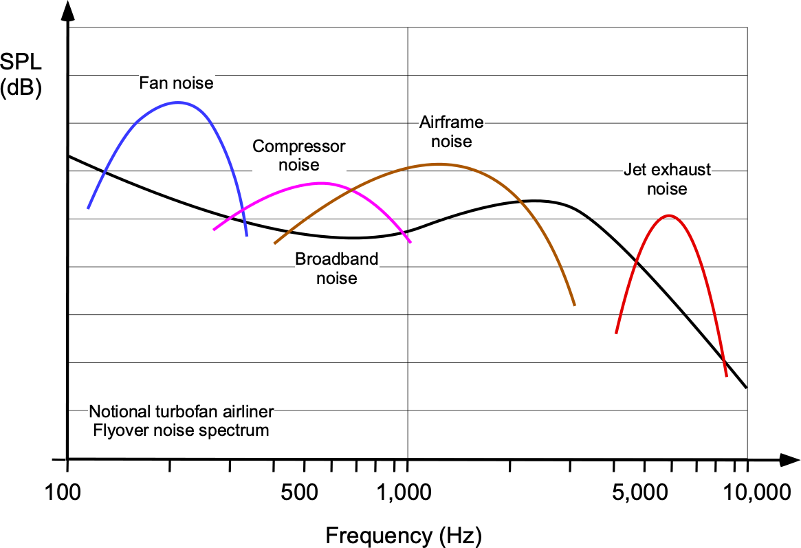
Aircraft noise originates from various sources associated with the operation and movement of an aircraft and can be broadly categorized into engine noise and airframe noise. The noise is then further classified into external noise (i.e., what an observer outside of the aircraft will hear) and internal noise (i.e., what an observer inside the aircraft will hear). The propulsion systems of aircraft, particularly jet engines, are significant contributors to external and internal noise during takeoff, climb, and landing, which usually occurs over a specific range of frequencies. Aerodynamic forces and turbulence created as the aircraft moves through the air also generate external and internal airframe noise, which again tends to appear distinctly in the overall noise spectra, a generic example being shown in the figure below.

The overall noise signature from an airplane is punctuated by specific noise sources that occur over a range of frequencies.

Airplane noise is dominated by engine noise, which contributes significantly to internal noise. Propellers can generate significant noise, especially when their tip speeds approach the speed of sound. However, the contribution of propeller-driven airplanes to the overall noise environment at airports is relatively less important than jet-powered aircraft. Airframe noise includes noise from the flow about the wings, fuselage, high lift devices such as flaps and slats, wing tips, undercarriage, and other structural components that protrude into the flow.

Jet Engine Noise

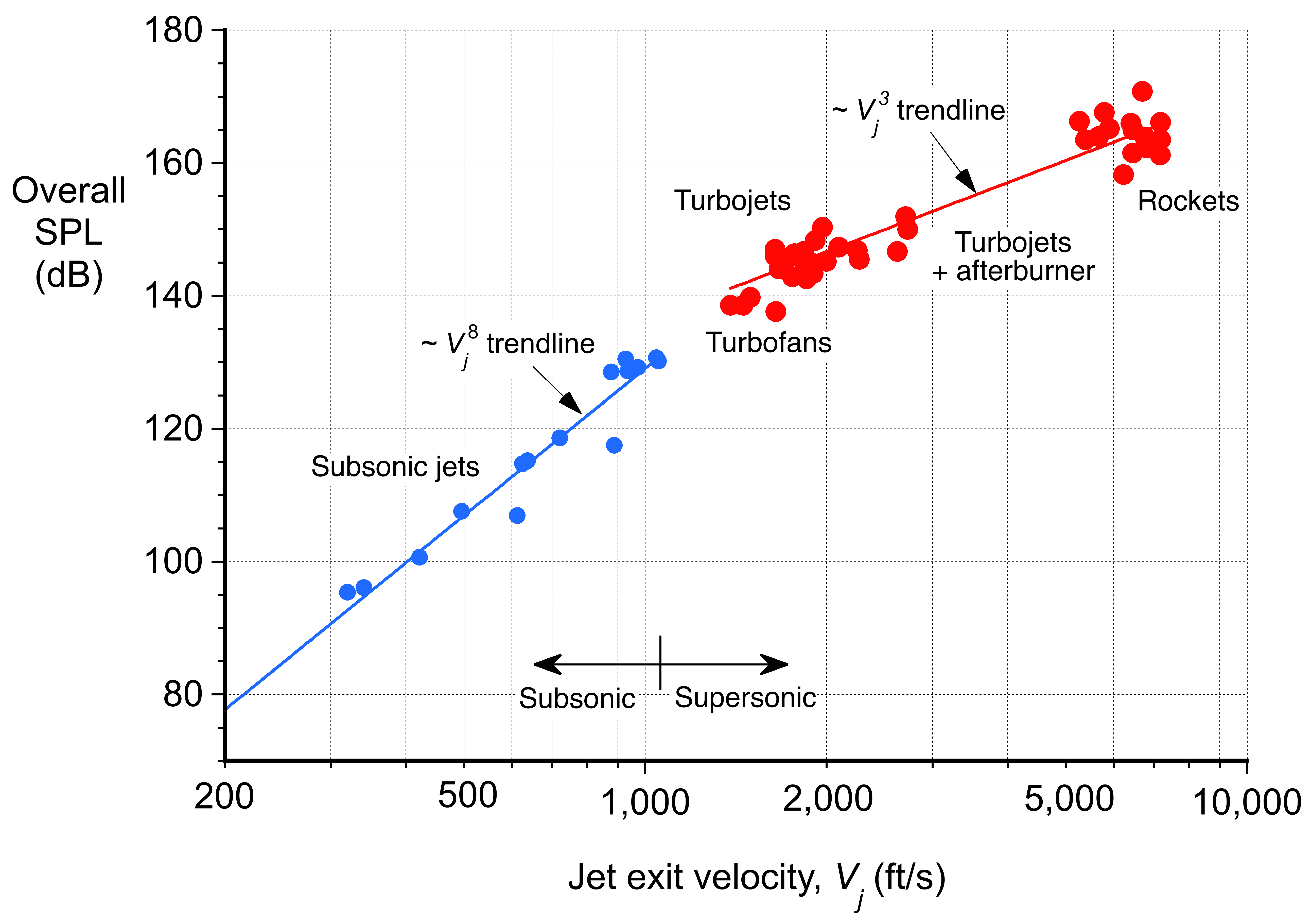
Jet engines generate most noise from the high-velocity exhaust gases expelled from the jet nozzle. It has been found that the noise generated by a turbojet increases very quickly with increasing the exhaust velocity. Research has shown that the increase in noise power is approximately proportional to the fully expanded exit velocity, $V_j$ , such that

(35) $\begin{equation*} L_W \, \propto \, V_j^n \end{equation*}$

where $n$ = 8 for subsonic jet conditions is called the eighth-power law, and $n$ = 3 for supersonic jet conditions is called the third-power law. Some measured results for turbojet and rockets are shown in the figure below, which confirm these approximate relationships. Turbojet engines also produce a more significant amount of noise in the higher-frequency range, increasing an observer’s annoyance level. While the jet velocity of a turbofan is much lower than that of a turbojet, the noise from the fan is still a significant source of low-frequency noise.

Jet engine noise for subsonic jet conditions follows an eighth-power law, and for supersonic jet conditions, a third-power law.

The differences in the design and performance of turbojet engines versus turbofans also affect the directivity of the noise from these engines, as illustrated in the figures below. The noise sources radiate as a series of overlapping radially symmetric lobes. The jet noise is directed downward and backward, whereas the intake noise from the compressor and fan is directed forward and downward. The compressor and jet turbine contribute significantly to the total noise of both types of engines. However, it can be seen that the jet exhaust noise is the dominant source for the turbojet.

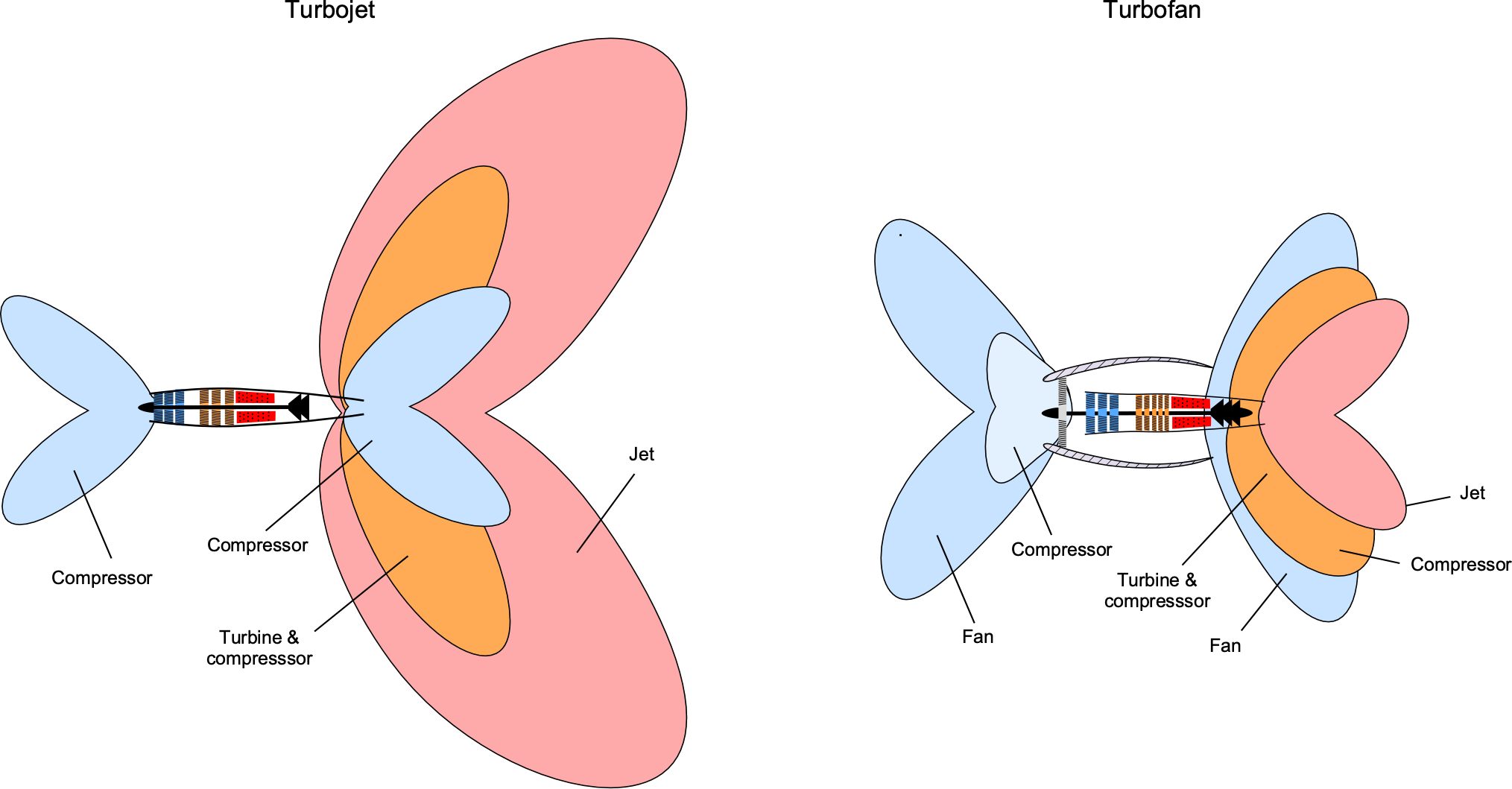
The differences in the design of turbojets versus turbofans affect the directivity of noise production.

The noise of a turbofan is distinctive for an observer on the ground listening to an airliner taking off. As the aircraft approaches, the low-frequency noise of the fan is dominant, but as the aircraft flies by, the noise is dominated by jet noise. The same effect can be noticed while sitting on the aircraft in flight. The fan noise dominates at the front of the aircraft, but at the back, the jet noise overwhelms other noise sources.

Listen to an airliner with turbofan engines taking off.

Propeller Noise

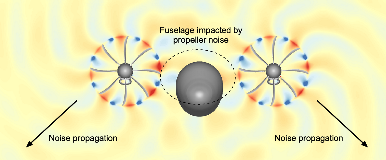
A propeller is a noisy device by any standard, although much has been done to quiet propellers on the most recent generations of aircraft. Like a helicopter rotor, the primary noise from a propeller comes from blade thickness, which produces a whishing noise, and the aerodynamic lift forces produced on the blades produce a more impulsive sound. Because these sound sources move with respect to a fixed observer, the sound waves coalesce along spiral wavefronts that radiate away from the propeller; an example is shown in the figure below.

Propellers produce noise wavefronts that spiral away from the aircraft at frequencies that can be particularly annoying to an observer.

The frequency of propeller noise relative to an observer, called the blade passage frequency (BPF), occurs at the product of the rotational frequency, $\Omega_p$ , and the number of blades, $N_b$ , $\Omega_{\rm BPF}$ , as given by

(36) $\begin{equation*} \Omega_{\rm BPF} =N_b \, \Omega_p \end{equation*}$

The sound frequency, $f_{\rm BPF}$ , will be

(37) $\begin{equation*} f_{\rm BPF} = \frac{\Omega_{\rm BPF}}{2 \pi} = \frac{N_b \, N_{\rm rpm}}{60} \end{equation*}$

where $N_{\rm rpm}$ the propeller rpm (revolutions per minute). For most propellers, the noise levels are high and occur in the frequency range where the ear is sensitive, i.e., between 500 Hz and 4,000 Hz. This is a similar range to much of the noise produced by a helicopter’s tail rotor.

Listen to what a piston-engine propeller airplane sounds like during takeoff.

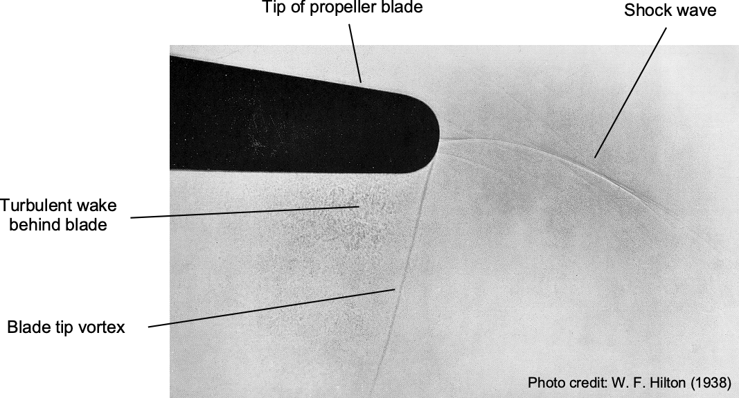
The rotational tip speed of a propeller, $V_{\Omega R}$ = $\Omega_p \, R_p$ , is also important regarding its noise production, where $R_p$ is the propeller radius. As supersonic tip Mach numbers are approached, the spiraling sound waves coalesce to become shock waves, increasing the amplitude, impulsiveness, and harshness of the propeller noise. The schlieren flow visualization image below, which is for a tip Mach number of 0.87, clearly shows the phenomenon. The tip vortex and the turbulent wake behind the blade are also visible, both of which will contribute to the noise produced by the propeller.

Schlieren flow visualization image showing the formation of a spiraling noise wave at the tip of a propeller.

Even if $V_{\Omega R}$ is kept low enough on a propeller so that the tip Mach number is significantly subsonic, as an airplane gains airspeed, $V_{\infty}$ , the helical velocity (and Mach number) at the blade tip will increase, i.e., by vector addition then

(38) $\begin{equation*} V_{\rm hel} = \sqrt{ (\Omega_p R_p )^2 + V_{\infty}^2 } \end{equation*}$

with the corresponding helical Mach number being given by

(39) $\begin{equation*} M_{\rm hel} = \frac{V_{\rm hel}}{a_{\infty}} \end{equation*}$

where $a_{\infty}$ is the local speed of sound.

Suppose the helical Mach number of the blade section exceeds the critical Mach number and becomes too close to one. In that case, noise will increase rapidly, and the propeller’s propulsive efficiency will also decrease. Measurements of propeller noise suggest that the noise in terms of SPL for a given thrust is linearly proportional to the tip Mach number, i.e.,

(40) $\begin{equation*} SPL_{\rm prop} \, \propto \, M_{\rm hel} \end{equation*}$

which seems to hold even for $M_{\rm hel} > 1$ . The main aerodynamic affecting propeller performance is shock-induced flow separation rather than the presence of shock waves. Therefore, this operating condition sets a limit to the useful operating envelope of the propeller.

Listen to what a turboprop airliner sounds like as it starts its takeoff roll.

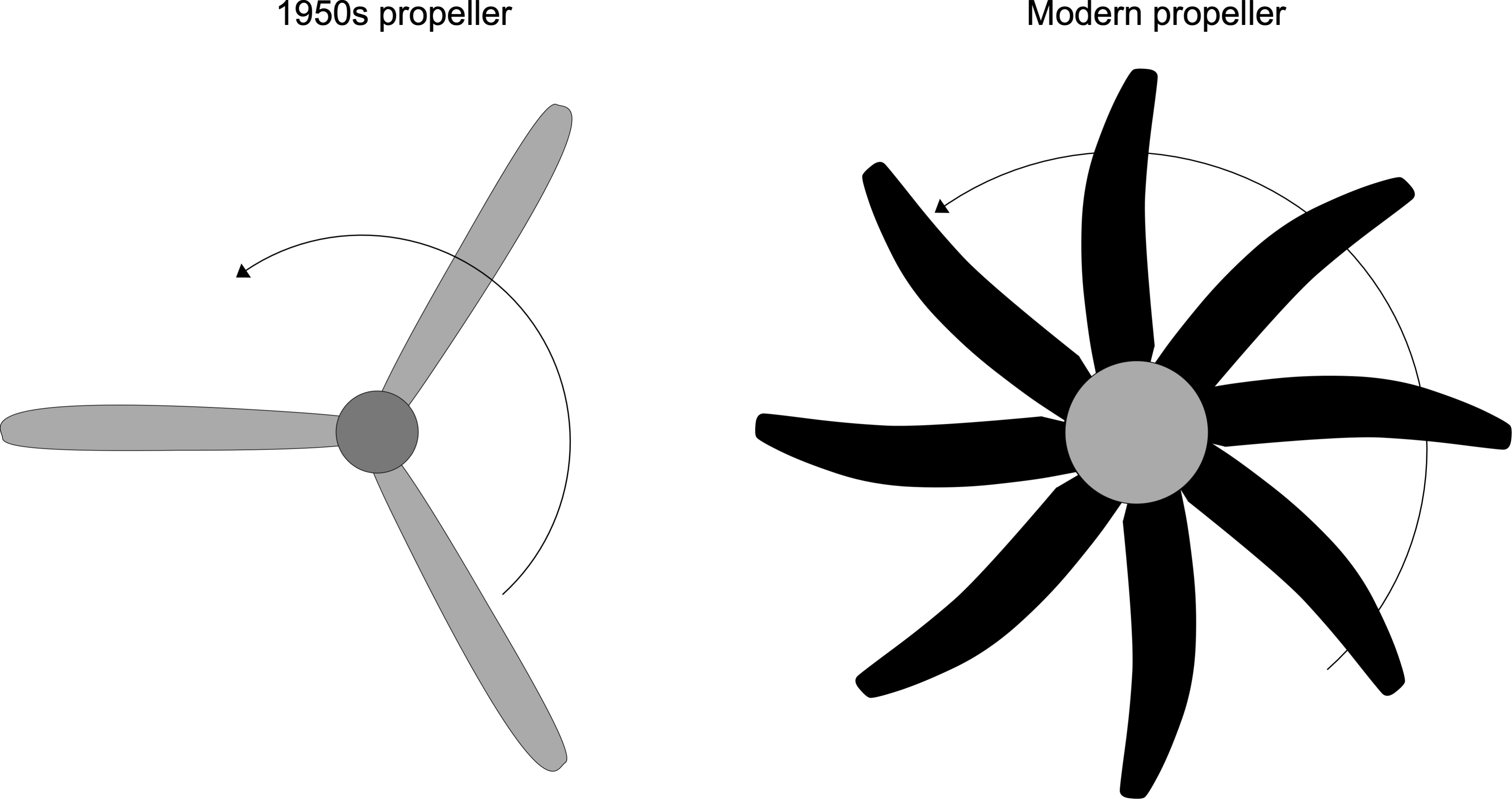
Strategies to reduce propeller noise include reducing the propeller rotational speed and increasing the number of blades. Another way to decrease noise levels is to take advantage of aerodynamics and design a swept blade, much in the manner done for helicopter blades, as shown in the figure below. The idea is that sweeping the blade reduces the incident Mach number normal to the blade’s leading edge, delaying the onset of supercritical flow and the build-up of shock waves.

Modern propellers use more blades with swept leading edges to help reduce noise and shift the noise to higher frequencies.

Airframe Noise

The deployment and retraction of flaps and slats during takeoff and landing contribute to aerodynamic noise. These devices alter the flow characteristics of the wings but also generate additional sound sources. Vortices trailed from the wing tips, flap side edges, and turbulence produced by flow separation over the flaps all contribute to noise. The undercarriage, when in the lowered position, is a significant source of turbulence and noise. During the landing and rollout, pilots may use reverse thrust to decelerate the aircraft on the runway, producing higher noise levels than during takeoff.
At cruising airspeeds at high altitudes, much of the internal cabin noise is airframe noise from the engines and the turbulent flow about the fuselage, which manifests as white noise. Various other aircraft systems and components contribute to the internal noise levels. These include noise from auxiliary power units (APUs), landing gear, hydraulic systems, air-conditioning systems, and other mechanical components.

Supersonic Noise

In recent years, there has been renewed interest in developing commercial supersonic aircraft, with startup companies exploring ways to make supersonic travel more sustainable and acceptable in terms of noise and environmental impact. Although no civil supersonic aircraft are currently flying, the high noise concerns associated with sonic booms must be addressed. Many military aircraft are capable of supersonic flight and can generate significant noise levels, including from their afterburners.

Listen to what a supersonic fighter aircraft sounds like on takeoff with its afterburner.

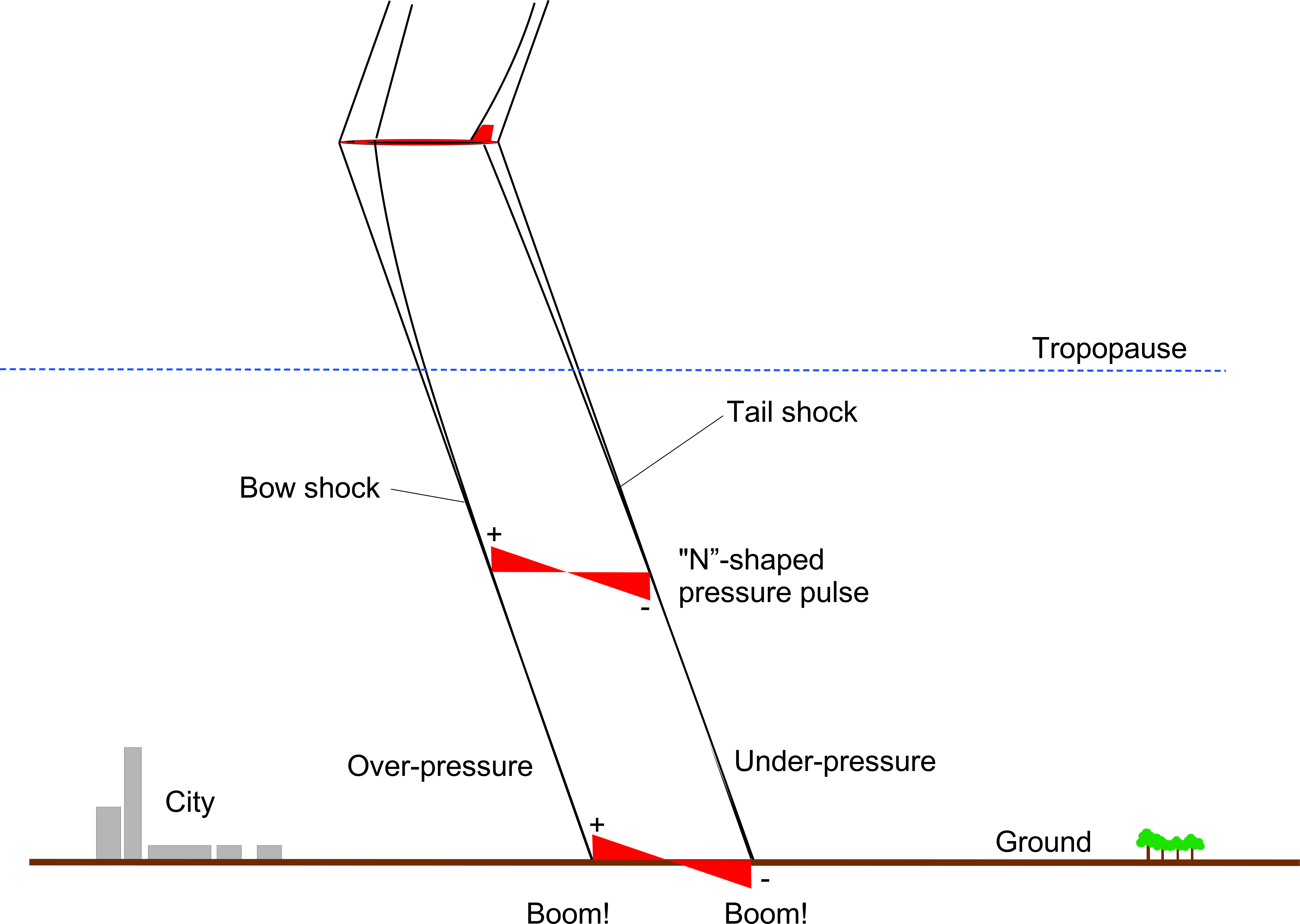
The noise produced by supersonic flight is characterized by the formation of sonic booms, as shown in the figure below. These are sudden and sharp changes in air pressure caused by the conical shock waves (called Mach waves) generated as the aircraft exceeds the speed of sound, i.e., Mach 1. When these shockwaves reach the ground, they produce a loud and distinctive “boom-boom” noise. Sonic booms are typically heard as a double “boom” because of the formation of Mach waves at both the nose and tail of the aircraft; the nose produces a compressor wave and an expansion wave at the tail. The signature of a sonic boom is intense, to the extent that the public will not tolerate it regularly.

The signature of a sonic boom is an “N” shaped pressure pulse, which can be loud and startling to an observer on the ground.

Listen to what Concorde sounded like at Mach 2 as it flew over a ship in the Atlantic Ocean.

Efforts have been made to address the environmental impact of supersonic flight, especially in terms of noise pollution. Researchers and engineers are developing technologies and aircraft designs that minimize sonic boom intensity and reduce engine noise. For example, designs like the low-boom supersonic aircraft aim to produce sonic booms at levels more acceptable to people on the ground. However, it remains to be seen if the sonic booms can be reduced to the level that would make a new generation of SST airliners realizable; limiting destinations to overwater routings will not be economically feasible for an airline.

Measuring Aircraft Noise

Several scales and metrics are used to assess and manage the noise impact of aircraft on the environment and human health. These scales consider factors such as the intensity, duration, and community impact of the noise produced by aircraft. There are two types of metrics:

Single events such as an aircraft flyover.
Cumulative events such as a day’s worth of aircraft flyovers.

Some of the metrics used for aircraft noise measurement and assessment include Sound Pressure Level (SPL), Noise Exposure Level (NEL), and Effective Perceived Noise Level (EPNL). The data obtained from these metrics also play a crucial role in developing regulations and noise abatement programs and focusing research to reduce the overall impact of aviation-related noise.

Sound Pressure Level (SPL)

As previously discussed, the Sound Pressure Level (SPL) measured in decibels (dB) is a fundamental metric for quantifying noise intensity, as given by Eq. 19. The SPL is commonly measured using a sound pressure meter (SPM), as shown in the photograph below,

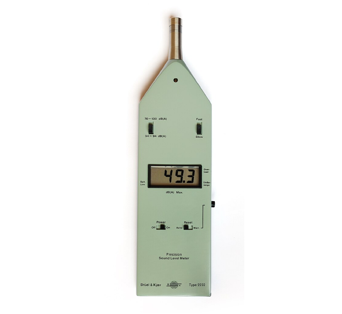
A Sound Pressure Meter (SPM) can measure noise directly in dB or dB(A). They are portable but can also be mounted.

The SPM is portable and can be placed at specific locations relative to the sound source, e.g., below an aircraft’s takeoff or landing path. The unit has a sensitive condenser microphone, which responds to changes in air pressure caused by sound waves. The voltage output from the microphone is amplified, filtered, converted to digital form, and displayed on the SPM as dB or dB(A).

Maximum Sound Level (MSL)

One single event noise metric type is the maximum sound level or $L_{\rm max}$ and is defined as the maximum sound level recorded during a specific sound exposure time. For example, consider the SPL measured below the flight path of an aircraft as it takes off, as illustrated below. The noise level will increase as the aircraft approaches, reach a maximum as it flies overhead, and then diminish as it flies away and climbs. The peak value of the SPL is called $L_{\rm max}$ .

The maximum sound level is defined as the maximum sound level recorded during a specific sound exposure time.

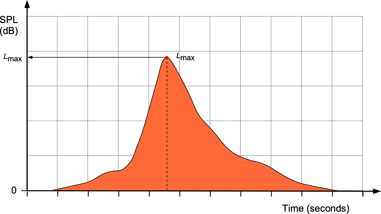
However, a limitation of using this value is that it does not account for the duration of the noise exposure, which will depend on the aircraft and how fast it is flying. The cumulative exposure to an observer will depend on how long the noise lasts, so the value of $L_{\rm max}$ conveys only limited information.

Sound Exposure Level (SEL)

This metric represents the cumulative acoustic energy (expressed in dB) of an individual noise event normalized to one second. SEL captures the noise level and the duration of a sound event in a single numerical quantity by summing all the noise energy from an event into an aggregate for one second, as shown in the figure below. This metric provides an unbiased comparison between noise events of various durations.

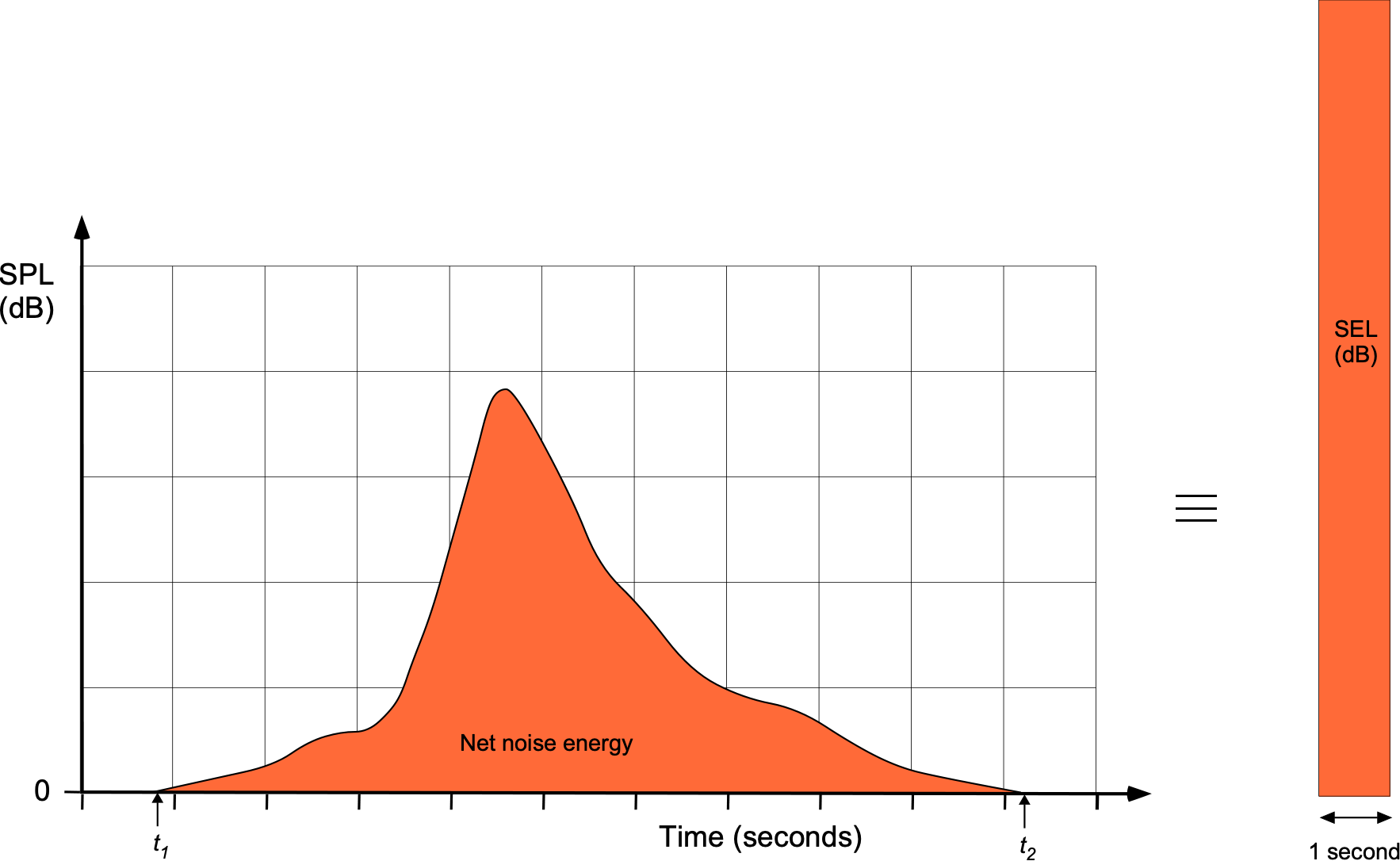
SEL captures the noise level and the duration of a sound event in a single numerical quantity by summing all the noise energy from an event into an aggregate for one second.

The value of the SEL is obtained by the integration of the time-varying sound pressure, $p(t)$ , between a start time $t_1$ and an end time $t_2$ using

(41) $\begin{equation*} \text{SEL} = 10 \log_{10}\left(\frac{1}{(t_2 - t_1)} \int_{t_1}^{t_2} p^2 (t) dt \right) \end{equation*}$

Inevitably, the pressure values are measured in dB using an SPM, so before the integration can be performed, they must be converted into linear pressure values using

(42) $\begin{equation*} p(t) = 10^{\frac{(L(t}{10}} \end{equation*}$

In practice, sound pressure values will be collected digitally at equal-spaced time points, $t_i$ , and stored in a data file for the interval $t_1$ to $t_2$ . Therefore, the value of SEL must be obtained using numerical integration. If the values of $\Delta t$ are sufficiently small, then the trapezoidal method of integration will be sufficient, i.e.,

(43) $\begin{equation*} \text{SEL} \, \approx \frac{1}{(t_2 - t_1)} \sum_{i=1}^{N} p^2(t_i) \, \Delta t \end{equation*}$

where $N$ is the number of discrete measurements, and $\Delta t$ is the time step between the measurements.

Remember that the SEL provides another form of noise measurement, in this case, to characterize total sound energy throughout the noise event. Therefore, it offers a useful way of assessing the potential impact of aircraft noise on individuals and the environment.

Single Event Noise Exposure Level (SENEL)

The single event noise exposure level (SENEL) is a variation of the SEL measurement. However, it is calculated only over the period when the level exceeds a selected threshold. But like the SEL, the SENEL is a metric that combines the intensity and duration of a single noise event. Therefore, the SENEL value allows an assessment of the impact of noise events that exceed a certain threshold, providing a more targeted evaluation of potentially disturbing or significant noise occurrences.

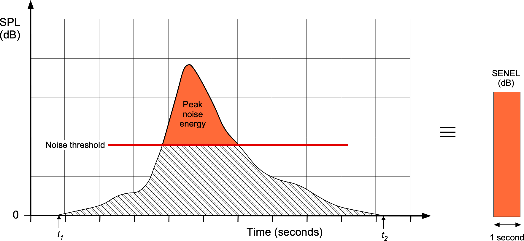
The SENEL combines the intensity and duration to assess the impact of noise above a certain dB threshold.

The relevant equation in this case is

(44) $\begin{equation*} \text{SENEL} = 10 \log_{10}\left(\frac{1}{(t_2 - t_1)}\int_{t_1}^{t_2} \max\left[p^2(t) - (L_{\text{th}})^2, 0\right] \, dt\right) \end{equation*}$

where the term $\max\left[p^2(t) - (L_{\text{th}})^2, 0\right]$ ensures that only the portions of the noise event exceeding the threshold $L_{\text{th}}$ contribute to the calculation. If the instantaneous sound pressure is below the threshold, that portion of the integral is set to zero. Again, the SENEL value would be determined by numerical integration, as previously explained for SEL.

Equivalent Continuous Noise Level (L_EQ)

The equivalent continuous noise level parameter L_EQrepresents the average continuous noise level over a specified period and is often used for environmental noise assessments. Its value can be obtained by making continuous noise measurements at frequent intervals throughout the day, as shown in the figure below. The period is often 24 hours, and the metric is denoted as L_EQ24h. However, L_EQ values for daytime and nighttime can also be determined, giving different values.

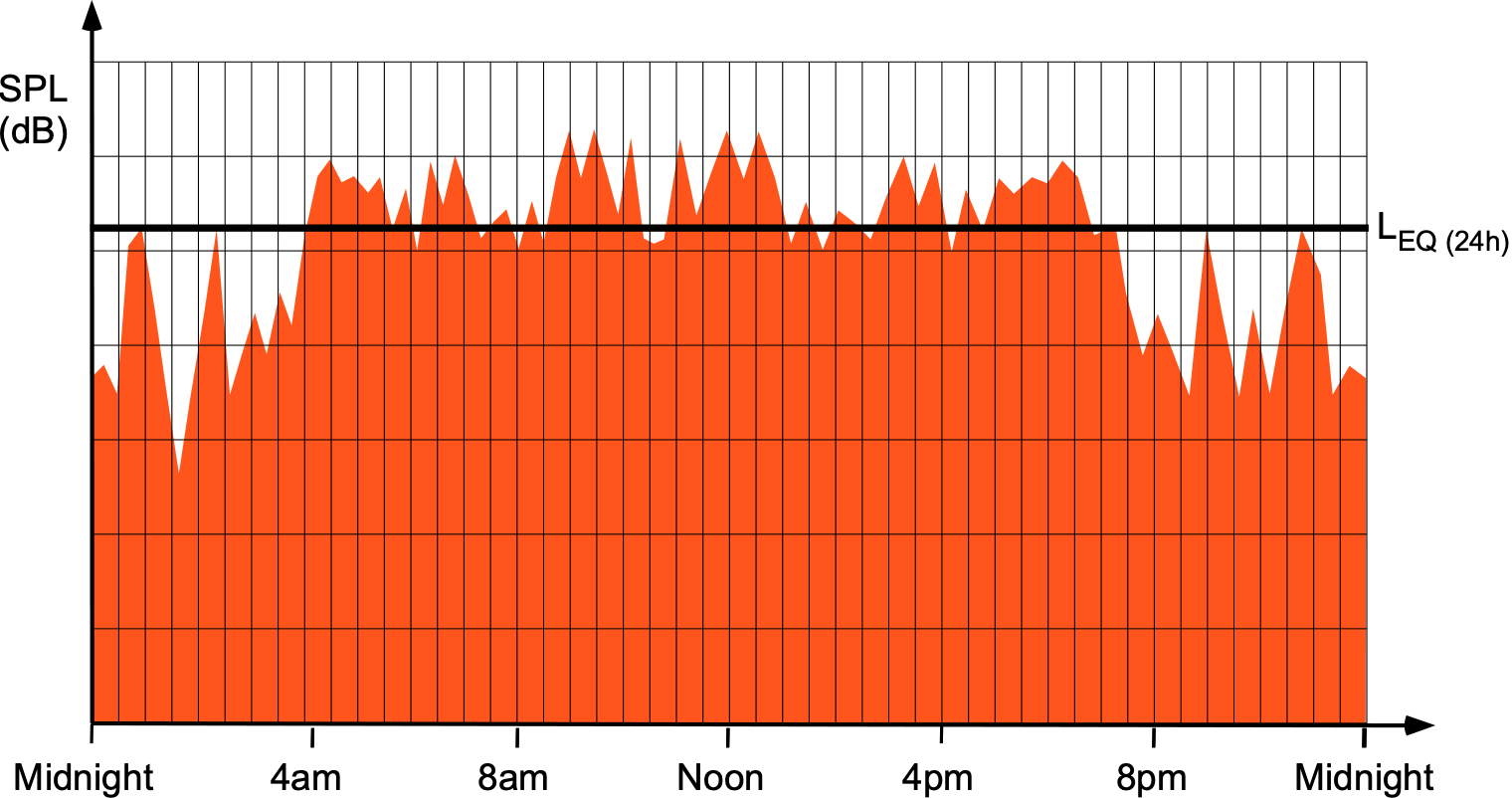
The LEQ represents the average continuous noise level over a specified period, usually a day.

For example, operations at an airport have quieter times and peak times. After midnight, passenger operations begin to slow down, except perhaps for infrequent cargo aircraft flights. Noise levels build up after 5 am, and passenger flights start for the day. There are usually several times when flight operations peak up, subsiding again after 8 pm.

The value L_EQ or L_EQ24h is calculated by integrating the square of the sound pressure over the specified time $T$ and then taking the square root, i.e.,

(45) $\begin{equation*} \text{L$_{\rm EQ}$} = \sqrt{\frac{1}{T} \int_0^T p^2(t) \, dt} \end{equation*}$

Therefore, if $T$ = 24 hours, the value of L_EQ24h will measure the average of noise over the 24 hours, delivering the same amount of noise energy as the actual, varying noise exposure. Once again, the integration would be performed numerically from discrete data.

Worked Example #5 – Calculating the Equivalent Continuous Noise Level (L_EQ)

Write a short piece of MATLAB code to show how to calculate the Equivalent Continuous Noise Level (L_EQ) in MATLAB using a set of raw dB sound level measurements. First, convert the dB values to dB(A). Hint: MATLAB has built-in functions for A-weighting, such as “A_weighting” in the Signal Processing Toolbox.

% Example sound level measurements in decibels at different time intervals
soundLevels = [80, 85, 90, 88, 92, 87, 89, 86, 91, 88];
% A-weight the sound level measurements
A_weighted_levels = A_weighting(soundLevels, ‘f’);
% Calculate the A-weighted equivalent continuous noise level (L_eq(A))
L_eq_A_weighted = 10 * log10(mean(10.^(A_weighted_levels / 10)));
% Display the result
disp([‘A-weighted Equivalent Continuous Noise Level (L_eq(A)): ‘, num2str(L_eq_A_weighted), ‘ dB’]);

Day-Night Average Sound Level (DNL)

The day-night average sound level, usually called DNL of $L_{\rm DN}$ ., is another metric used for assessing the long-term impact of noise, particularly in residential areas near airports. It is the same as LEQ but with a 10 dB penalty applied to the measurements occurring during nighttime to account for people’s increased sensitivity to noise.

Remember that one cannot add noise levels in dB, so the weighted dB measurements, usually in dB(A), must be converted to pressures or intensities. The relevant equation is

(46) $\begin{equation*} \text{DNL} \equiv L_{\rm DN} = 10 \log_{10} \frac{1}{T} \left( \int_{\rm day} 10^{ \frac{( \rm{dB(A)} + 10)}{10} } \, dt + \int_{\rm night} 10^{\frac{\rm{dB(A)}}{10}}\, dt \right) \end{equation*}$

The nighttime hours are typically from 10:00 pm to 7:00 am.

The DNL noise metric is the standard for all FAA studies of aviation noise exposure in airport communities. DNL measurements consider the amount of noise from each aircraft movement (takeoff or landing) and the total number of movements throughout the day. Therefore, a few relatively loud flight movements can result in the same DNL as large numbers of relatively quiet movements, which the FAA believes is the fairest way to assess the noise levels at any airport. The FAA uses the DNL metric to set standards and policies.

Community Noise Equivalent Level (CNEL)

The Community Noise Equivalent Level (CNEL) metric is similar to the DNL metric but with a 5 dB noise penalty added to measurements made during the evenings from 7 pm to 10 pm. The relevant equation is

(47) $\begin{equation*} \text{DNL} \equiv L_{\rm DN} = 10 \log_{10} \frac{1}{T} \left( \int_{\rm day} 10^{\frac{( \rm{dB(A)} +10)}{10}} \, dt + \int_{\rm evening} 10^{\frac{(\rm{dB(A)}+5)}{10}} \, dt + \int_{\rm night} 10^{\frac{ \rm{dB(A)}}{10}} \, dt \right) \end{equation*}$

which, yet again, would be calculated numerically from discrete noise measurements.

Effective Perceived Noise Level (EPNL)

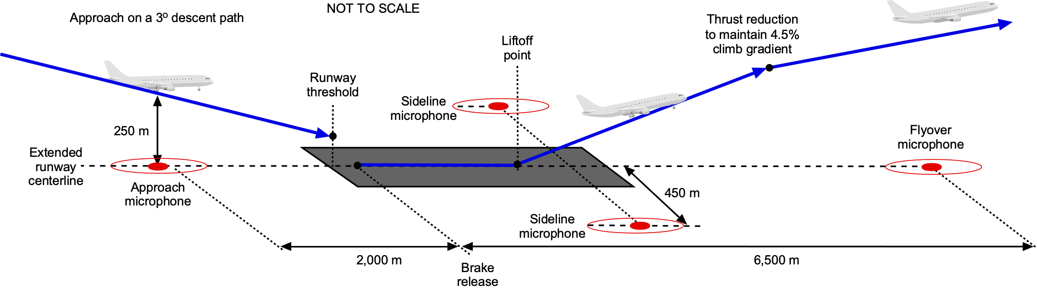
The effective perceived noise (EPN) or effective perceived noise level (EPNL) is a metric used in aircraft noise certification processes. The ICAO defines the EPNdB (EPN in units of decibels) as a single-number rating that reflects the perceived noisiness of any given aircraft. In this regard, the FARs “Part 36 – Noise Standards: Aircraft Type and Airworthiness Certification” define instrumentation requirements and test procedures for aircraft noise certification.

The instrumentation needed consists of certified microphones, recording equipment, calibrators, analysis equipment, and other items. For subsonic transports and turbojet-powered airplanes, the microphones are located at reference points on the extended centerline of the runway, 6,500 m from the start of the takeoff roll, 2,000 m from the approach threshold to the runway, and on the sidelines 450 m from the runway, as shown in the figure below. Noise levels are then measured at each point.

Summary of microphone locations used for the certification of a civil aircraft.

While there are several steps used to determine the certification value of the EPNdB, the general formula is of the form

(48) $\begin{equation*} \text{EPNL} = \int \text{A-weighted noise spectrum} + \text{corrections} \end{equation*}$

where the corrections include allowances for annoyance, tone, and duration. The final single value used for certification is then determined.

The certification noise limits depend on the aircraft, including its gross takeoff weight. Aircraft manufacturers typically work closely with aviation authorities to ensure compliance with noise certification standards during the design and certification process. Older aircraft may be “grandfathered” from the current noise limits, but constraints may be placed on where and when they can operate.

Listen to what it sounds like as a jetliner flies overhead.

The overall goal of using the EPNL as a metric is to maintain and reduce the perceived noise impact of aircraft operations near airports and in populated areas. All aircraft manufacturers must conduct noise certification tests to determine the noise levels their aircraft models produce. These tests involve measuring noise during takeoff, approach, and other conditions. The results are then used to verify the noise of the aircraft is below the required thresholds to comply with the FARs and gain aircraft certification.

Noise Contour Maps

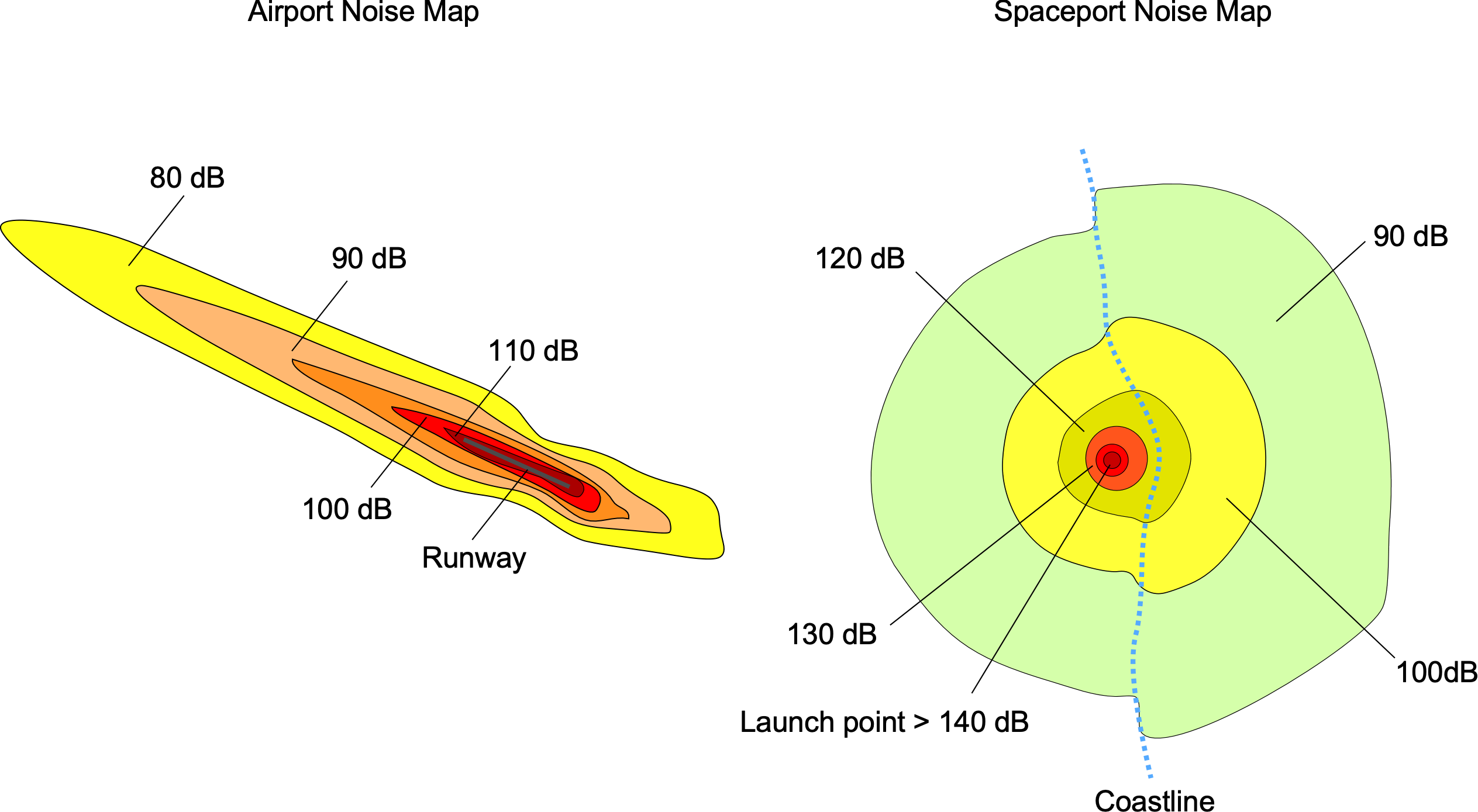
Noise contour maps visually represent the spatial distribution of noise levels around airports and spaceports. These maps use contours to indicate areas with similar noise exposure. Noise levels can be computed at individual locations of interest, but to show how noise can vary over extended regions, noise metric results like DNL are often drawn on contour maps with the same levels in dB(A), as shown in the figure below.

The shape of the noise contours at an airport depends on many factors, but they are influenced primarily by aircraft approach and departure paths. Different aircraft have varying noise profiles, and the map may consider the types and frequencies of aircraft movements. Terrain avoidance or noise abatement flight paths will change the contours so that every airport will have a different noise contour map.

Noise contour maps are often used to assess compliance with established noise standards and guidelines set by aviation authorities. Noise contour maps are crucial for planning land use around airports to minimize the impact on residents and sensitive areas. Authorities may establish zoning regulations based on noise levels to control development in high-noise areas.

Contour maps for spaceports serve a similar purpose as those for airports but focus on the spatial distribution of noise generated by space launch activities. The primary noise source at spaceports is from rocket launches. The intensity and duration of the noise generated during launch vary based on the type of rocket, propulsion system, and other factors.

Spaceports handling rocket landings or suborbital flights and sonic booms during re-entry or descent phases may also contribute to the shape and magnitude of the noise maps. With the emergence of commercial space tourism, the impact of rocket noise on both residents near launch sites and tourists in the vicinity is becoming a subject of interest. Balancing the excitement of space exploration with the need to minimize noise impact is a crucial challenge.

Noise Propagation

The propagation of aircraft noise will be a function of several factors, including relative distance and direction from the aircraft to the observer, atmospheric attenuation from wind, humidity, and temperature, and noise barriers (e.g., hills, mountains, large stands of trees, and buildings). Recall that a primary effect of noise propagation is the spherical spreading of the acoustic energy, accounting for a decrease in acoustic intensity of approximately 6 dB for each doubling of relative distance.

Water vapor in the atmosphere is relatively effective at absorbing and attenuating noise. Also, the higher noise frequencies are more readily absorbed. For this reason, high-frequency noise typically decreases with distance more rapidly than midrange or low-frequency noise. Absorption has the most significant influence on noise propagation for flying aircraft.

Atmospheric temperature gradients also affect aircraft noise propagation. During periods of average temperature gradients, where air temperature steadily decreases with increasing altitude, aircraft noise is mostly deflected upward, producing areas of little or no noise on the ground at specific distances from the aircraft. During an atmospheric temperature inversion, the reverse situation is true, and aircraft noise tends to be deflected downward, thus increasing noise at ground level.

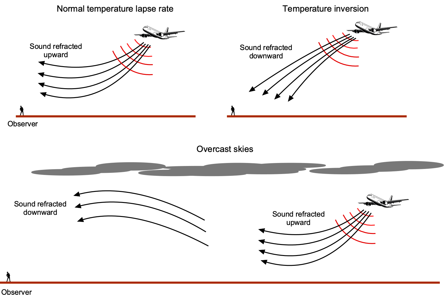
The propagation of aircraft noise will depend on the local atmospheric properties, amongst other factors, including winds and terrain.

During low-level aircraft operations, surface absorption and deflection may decrease noise levels at low observation angles. Intervening objects (e.g., hills, buildings) will also affect noise propagation and may cause echoes. Cloud layers may also affect noise propagation, reflecting and focusing it over longer distances. These effects must be considered when measuring noise and how the results are interpreted or corrected.

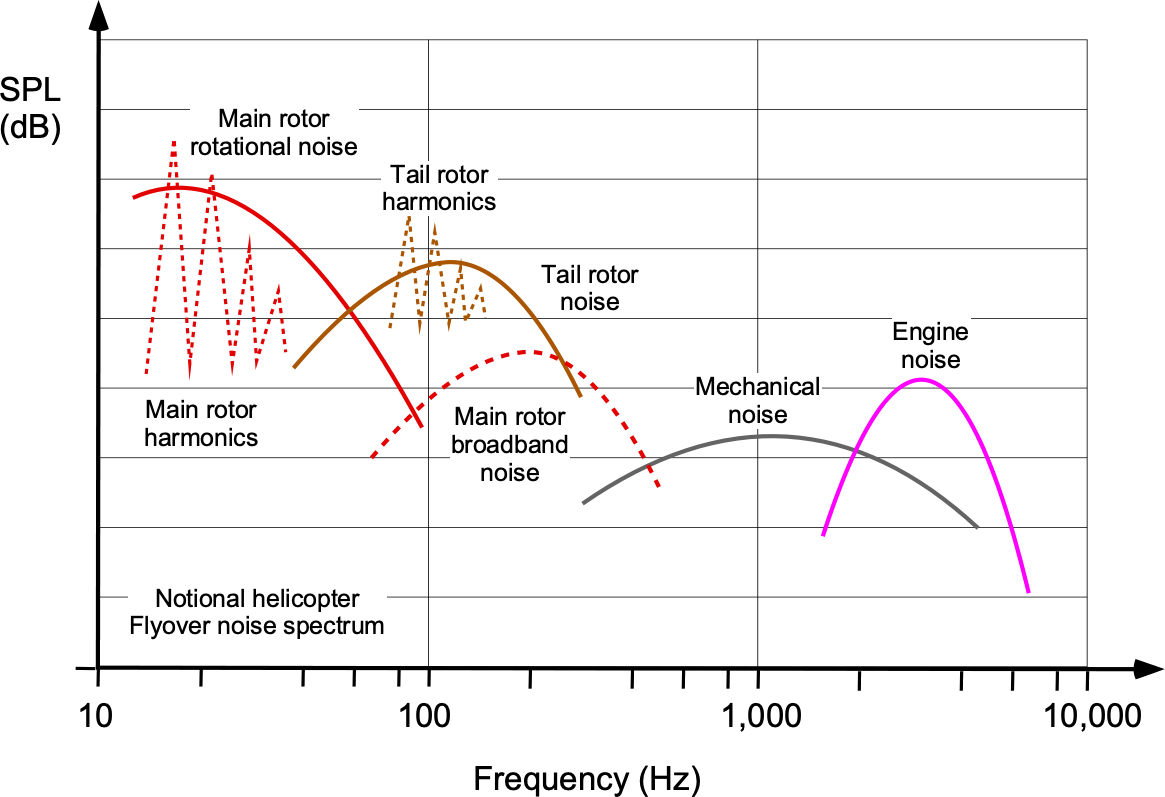
Helicopter Noise

Observers usually perceive helicopters as being a particularly noisy type of aircraft. Helicopters produce distinctive noise patterns from their main and tail rotor blades, as shown in the figure below. Helicopters typically have a primary rotor responsible for lift and thrust and a tail rotor for anti-torque to counteract the rotational forces induced by the main rotor. Both rotors contribute to the overall noise signature of a helicopter. The rotational tip speed (especially Mach number), blade design, and tip shape influence the rotational noise. Engine noise also significantly contributes to the overall noise signature of a helicopter, with the whine of turboshaft engines appearing in the higher frequency range.

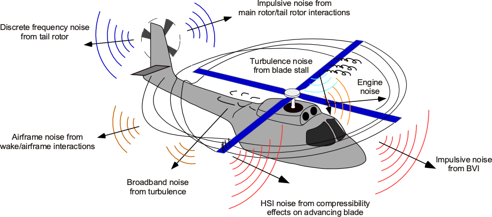
A helicopter has a plethora of source sources, which results in a complex noise field with localized regions of strong directivity.

As the rotor blades rotate, they generate lift and thrust and produce aerodynamic noise, including blade-vortex interactions (BVI) and turbulent flow. BVI occurs when the helicopter’s rotor blades interact with the vortices shed from the tips of preceding blades. This phenomenon generates distinctive impulsive noise, often described as a “thump-thump” sound, and is most pronounced during descent or low-speed flight. BVI noise is directed downward and forward away from the rotor. As the same suggests, broadband noise occurs over a broad range of frequencies and is not distinguished by discrete frequencies or individual tones.

Listen to what a helicopter sounds like.

Primary sources of discrete frequency noise come from the main and tail rotor blades, which occur at the product of their rotational frequency and the number of blades, called the blade passage frequency. For a rotor, if the rotational speed is $\Omega$ and $N_b$ is the number of blades, then

(49) $\begin{equation*} \Omega_{\rm BPF} = N_{b} \, \Omega \end{equation*}$

The resulting noise frequency, $f_{\rm BPF}$ , will be

(50) $\begin{equation*} f_{\rm BPF} = \frac{\Omega_{\rm BPF}}{2 \pi} \end{equation*}$

As shown in the figure below, the blade passage frequencies of the main rotor and tail rotor, which are different, are dominant in the overall noise spectrum. The helicopter’s main rotor noise occurs at a much lower frequency than any propeller, and the characteristic “thump-thump” noise below 100 Hz is very annoying to an observer. This is particularly true for the older helicopters with two or three blades, where the noise may be “felt” rather than heard. Such low-frequency sound waves are not absorbed much in the atmosphere, so they also propagate to long distances; one can often hear helicopters approaching an airport much further away than any airplane.

A helicopter’s main and tail rotors dominate its overall noise spectrum.

As the helicopter flies forward, the advancing blade tip will see higher flow velocities and Mach numbers, resulting in a noise source called HSI, as already mentioned. HSI noise tends to be directed forward and downward, and like BVI noise, it tends to be impulsive and occurs at the blade passage frequency, which can be very annoying.

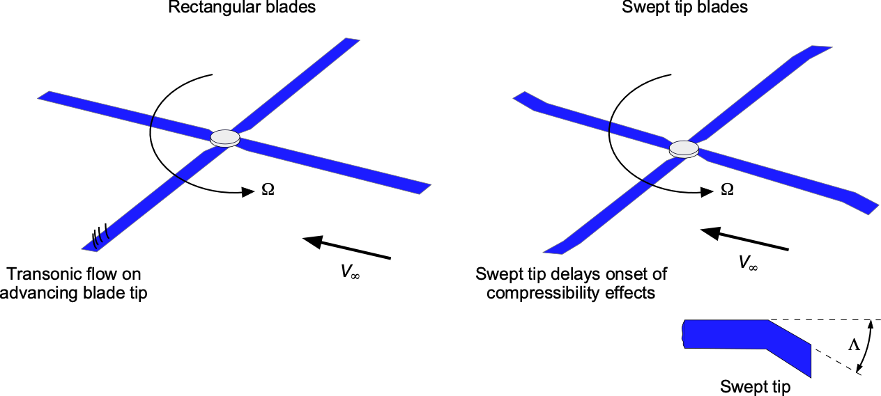
High-speed impulsive noise (HSI) can be mitigated to some extent by using rotor blades with swept tips. Most helicopter manufacturers will use variations of the basic concept.

Ongoing research and technological advancements aim to mitigate helicopter noise. These include modifications to rotor blade designs. HSI noise can be mitigated to some extent by using a swept leading edge at the tip and reduced thickness-to-chord ratio, and most modern helicopters will have such design features. This method works the same way as sweeping the wing of a high-speed jet airplane; the increased sweep near the blade’s tip delays the formation of supercritical flow and shock waves.

Noise Concerns for Military Aircraft

In military aviation, noise plays a crucial role in the detectability of aircraft. Low-noise aircraft, often designed with stealth features, provide tactical advantages by reducing their acoustic signatures. Stealth operations benefit from minimized noise emissions, enhancing the ability to approach targets covertly and maintain operational security. However, achieving complete noise elimination is a complex task, as it involves trade-offs with engine performance, and some mission requirements may necessitate operating at higher noise levels.

The continuous evolution of sensor technologies also poses challenges, as even relatively quiet military aircraft may now be detected by advanced acoustic sensors. Balancing the need for reduced noise with performance and operational capabilities remains crucial in military aircraft design and strategy.

UAV & Drone Noise

Noise mitigation is likely among the most challenging issues in the emerging Urban Air Mobility (UAM) and drone industry, i.e., those designated as Unoccupied Aerial Vehicles (UAVs). It is unrealistic to think that hundreds or thousands of drones or UAM air taxis shuttling commuters around cities and in the suburbs will not create a backlash from the general public about their noise levels. Most drones and UAVs are driven by small rotors turning at relatively high rotational speeds, creating BPF values much higher than helicopter rotors and higher than conventional propellers. These frequencies also tend to be in the range where the human ear is most sensitive, i.e., between about 1,000 Hz and 4,000 Hz, so the perception of noise is likely greater.

Listen to what a drone sounds like when it’s hovering.

For now, the standards for the noise certification of UAVs and drones will likely be based on the effective perceived noise level, or EPNL, in the same manner used by airplanes and helicopters. Even if UAVs can meet these standards, other metrics may be needed with the large number of aircraft in the airspace simultaneously and close together. The FAA will likely have to establish some new form of community noise equivalent level metric and day-night average sound level metrics specific to UAV operations. However, at this point, the noise standards for UAVs of all types still need to be defined.

Rocket Noise

Rockets are the loudest sound source humans can experience, except perhaps at an AC/DC rock concert! Rocket noise, often called launch noise or rocket acoustic environment, is generated during the various phases of rocket launches. This noise originates mainly from the high-speed ejection of gases from the rocket engines. The reason is that the exhaust plume’s interaction with the surrounding atmosphere produces Kelvin-Helmholtz instabilities (vortices) and turbulent flow, consequently creating intense acoustic pressure waves, as shown in the figure below.

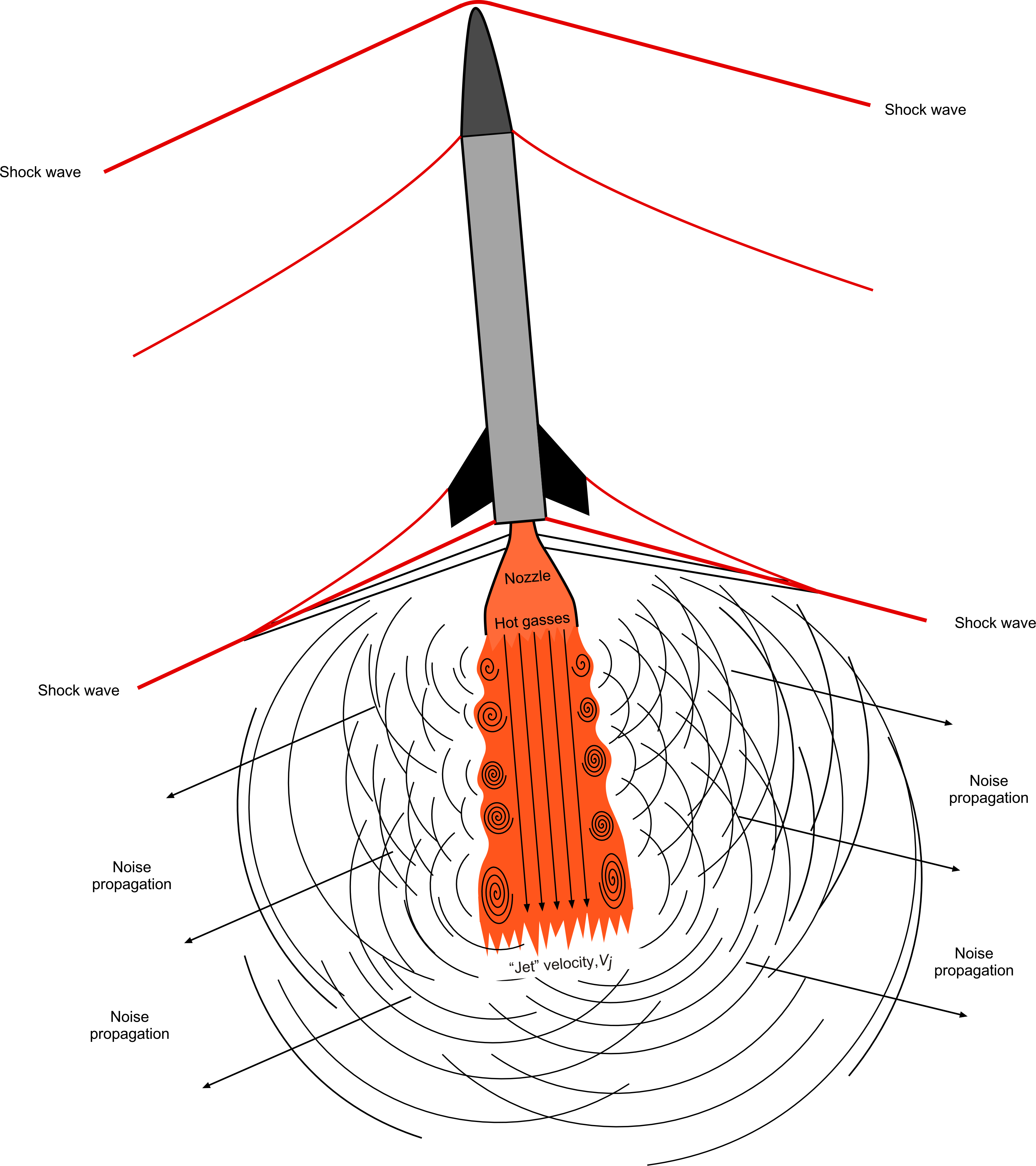
A rocket launch is a noisy affair, which originates mainly from the supersonic jet exhaust and the formation of wake instabilities.

The noise is radially directional, with the highest noise levels at an angle of about 40 to 50 degrees from the direction of the exhaust flow. The design and configuration of the launch vehicle will also influence the noise it generates, e.g., the number and type of engines, as well as the geometry of the rocket, will impact the acoustic signature during liftoff and ascent. Rocket noise is most prominent at liftoff because the rocket’s engines operate at maximum thrust, and some noise is reflected from the ground. The overall noise levels from a rocket may exceed 140 dB within several miles of the launch pad and will reach the threshold of pain. The residual noise from a launch may be heard over 50 miles (80 km) away. Noise pressure waves can also cause significant acoustically induced vibrations on the launch vehicle and the surrounding infrastructure, even damage, besides other issues.

Listen to the extreme noise produced by a NASA Space Shuttle! WARNING: Play first at a low volume.

Sonic booms from the shock waves as the vehicle exceeds Mach 1 in the atmosphere may also be produced and heard by an observer located below or near the launch path. However, these paths are usually over the ocean and will only affect a reasonably narrow region that is perhaps ten to 30 miles wide. The shock waves are more likely heard near the returning flight path of a reusable first stage. Rocket noise, particularly sonic booms, can be startling to humans but tolerable if expected.

The geographical and environmental characteristics of the launch site play a role in how rocket noise propagates. Coastal areas, for instance, can affect how sound waves travel over water, influencing the impact on nearby communities. Rocket noise may have some disruptive effects on wildlife, such as at the Kennedy Space Center, where during 2022, a launch occurred on average every six days. Like aircraft noise, rocket noise is measured using sound level meters at monitoring stations around launch sites, which routinely measure noise levels, frequency characteristics, and temporal patterns. The FAA has established guidelines and regulations to manage the environmental impact of rocket launches, including noise considerations, but does not impose noise limits or restrictions in the manner done for aircraft.

Internal Noise

Internal aircraft noise is generated within the cabin or interior during flight. Internal aircraft noise can affect the comfort and well-being of passengers and crew members, and various factors influence it. The sound of aircraft engines can penetrate the cabin, especially in smaller or older aircraft. The airflow around the aircraft, particularly during takeoff and landing, can contribute to noise inside the cabin. Changes in altitude can affect the aerodynamic and engine noise, influencing the overall noise environment in the cabin. Mechanical vibrations from various aircraft components, such as landing gear, can also be transmitted to the cabin, creating noise.

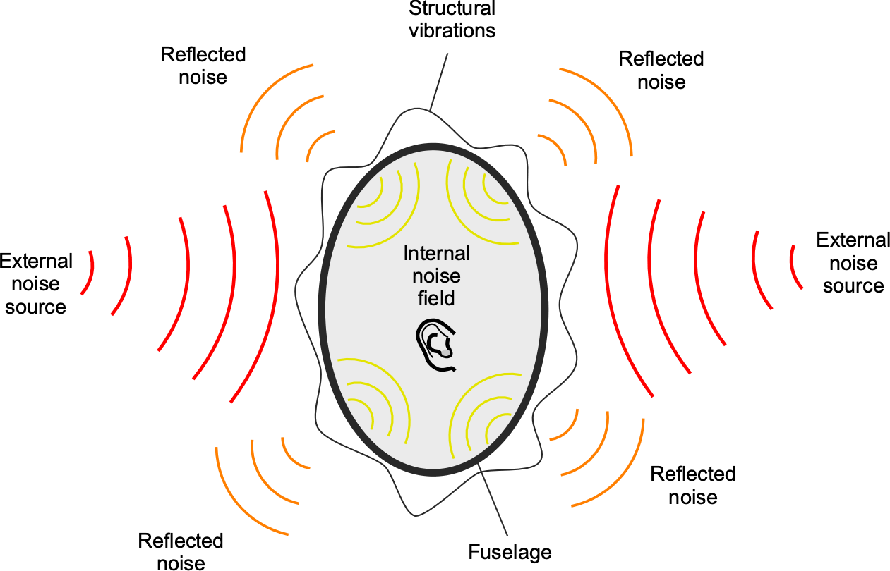
The sound transmission loss, $TL$ , is a quantity that measures the proportion of the incident sound power, $W_I$ , to the transmitted sound power, $W_T$ . It can be calculated using

(51) $\begin{equation*} TL = 10 \log_{10} \left( \frac{W^l}{W^T} \right) \end{equation*}$

Therefore, the transmission loss gives a quantifiable metric that can be used as a guideline to help quieten the inside of the fuselage. It is also a function of the frequencies of the exciting sound waves. The stiffness properties of the structure dominantly govern the low-frequency sound transmission loss through fuselage structures. Low-frequency noise, such as propeller noise, is difficult to insulate from. Hence, it is essential to identify the effects of the stiffness variables on the low-frequency sound transmission loss through the fuselage. Remember that noise insulation materials will be needed, but they also add to the aircraft’s empty weight.

During cruise flight in jet airliner, most of the noise is broadband “white” noise generated by the turbulent boundary layer along the length of the fuselage. Most passengers on long-haul flights will also use noise-canceling headphones or earplugs to enhance comfort and reduce the impact of cabin noise, which is a contributing factor to the malady known as jetlag.

Listen to what it sounds like inside a commercial jetliner during cruising flight.

The design and quality of insulation materials in the aircraft’s structure influence how much external noise enters the cabin. The materials used in the interior, such as seats, walls, and ceiling panels, can affect the transmission of noise. The overall design of the aircraft, including the fuselage structure and windows, plays a role in determining internal noise levels. New insulation materials and design features have significantly reduced external noise transmission into the cabin.

Listen to what it sounds like inside a turboprop airliner during takeoff, climb, and cruise.

Continuing attention by aircraft manufacturers is being placed on understanding and mitigating airframe and engine noise to reduce internal noise. Reducing the complexity and irregularities of the exterior surfaces can help minimize some types of airframe noise. This will likely involve optimizing the aerodynamic design of wings, fuselage, and interfering components to reduce turbulence. Active flow control technologies could also manipulate the airflow around the aircraft surfaces, although these are far from practical implementation. Using sophisticated computational tools, such as computational fluid dynamics (CFD), continues to aid in simulating and analyzing the airflow around different aircraft components to help reduce internal noise.

Aircraft Noise Mitigation & Control

Many regulations are in place to control noise emissions from aircraft. Aircraft noise is not limited to the air; ground operations, including taxiing and maintenance activities, can contribute to noise levels in and around airports. Efforts to mitigate the impact of aircraft noise often focus on addressing the sources of noise discussed in this chapter. The idea is to reduce the overall noise footprint as it would affect people on the ground without impacting other aspects of the aircraft’s performance. On the one hand, certain flight operations, such as changes in altitude or direction instructed by air traffic control, can result in more noise as the aircraft adjusts its flight path. On the other hand, operational procedures and flight path optimization can also play a role in minimizing the impact of aircraft noise.

Today, efforts to control and mitigate aircraft noise continue to involve a combination of regulatory measures and technological advancements, with noise reduction goals set by the ICAO. Regulatory bodies, such as the Federal Aviation Administration (FAA) in the United States, have established noise certification standards for all aircraft types. These standards limit the noise emissions of new aircraft to minimize the environmental impact. As with other forms of transportation, community engagement is crucial in addressing concerns related to helicopter noise. Collaborative efforts between helicopter operators, regulatory authorities, and local communities can lead to the development of effective noise abatement strategies.

Ongoing research explores the potential of emerging technologies, such as electric propulsion systems and distributed propulsion, to reduce aircraft noise. These technologies aim to provide more efficient and quieter options. In the long term, understanding and addressing aircraft noise must involve a combination of engineering advancements, regulatory measures, and operational considerations.

Summary & Closure

By most standards, aircraft, in general, are still considered by the general public as being excessively noisy. The noise generated by aircraft is particularly high near airports and military bases and has implications for the environment and human health. Much progress has been made since aircraft noise problems peaked during the 1960s after the introduction of turbojets and noise regulations were introduced. Since then, average jetliner noise levels have been reduced significantly using turbofan engines, and levels can be expected to be reduced further as new generations of turbofan engines are introduced.

However, because the impact of aircraft noise also depends on how often the noise occurs, the amount of noise reduction needed for each aircraft becomes more significant as the number of flights increases. Indeed, the aircraft community still has much work ahead to confine objectionable aircraft noise within the boundaries of an airport, which will depend on the airport’s size, aircraft fleet mix, and actual growth in air travel.

As the field continues to advance, proactive engineering efforts to minimize the impact of aircraft noise are integral to the industry’s mission to ensure that new aircraft will comply with increasingly stringent noise regulations in the future. Emerging technologies such as electric propulsion are also being explored further to mitigate the noise and environmental footprint of air travel. Reducing rocket launch noise is also an important goal but a remarkably complex challenge because of the high intensity, broad frequency spectrum, and diverse types of propulsion systems that are being used.

5-Question Self-Assessment Quickquiz

For Further Thought or Discussion

How is aircraft noise measured and characterized in terms of decibels and frequency?
What are the primary noise sources in an aircraft, and how do they contribute to overall noise levels?
Explain the concept of noise footprint and its significance in assessing the impact of aircraft noise.
Discuss the potential health effects of long-term exposure to aircraft noise on nearby communities.
What regulatory frameworks are in place to mitigate the environmental impact of aircraft noise, and how effective are they?
Explore the current advancements in aircraft noise reduction technologies.
How do innovations like quieter engines and aerodynamic modifications reduce noise levels?
Discuss the challenges associated with implementing noise reduction technologies in existing aircraft fleets.
What strategies are airports and aviation authorities using to engage with local communities affected by aircraft noise? How effective are these strategies in addressing community concerns?
How can urban planning contribute to minimizing noise exposure for residents?
Compare and contrast the approaches taken by different countries to address the issue of aircraft noise.

Other Useful Online Resources

Visit the following websites to learn more about sound and aircraft noise issues:

Understanding sound waves.
Visualizing sound waves and cymatic responses.
What is sound? The fundamental science behind sound.
An example of aircraft noise pollution in the London suburbs.
FAA Office of Environment and Energy
SFO tests system to reduce flight noise in nearby neighborhoods
ICAO Environmental Protection.
The noise produced by early jet airliners.
NASA Aeronautics Noise.
Noise produced by a Convair 990 airliner.
EASA Environment.
USAF F-16 full afterburner takeoff!
ACRP Reports.
How noisy is a glider? Not so much!
ACI World – Environment.
Yes, helicopters are noisy!
EPA Aviation Noise Reduction.
Listen to some propeller noises!
AECR Publications.
IATA Environmental Initiatives.

License

Icon for the Creative Commons Attribution-NonCommercial-NoDerivatives 4.0 International License

Introduction to Aerospace Flight Vehicles Copyright © 2022, 2023, 2024 by J. Gordon Leishman is licensed under a Creative Commons Attribution-NonCommercial-NoDerivatives 4.0 International License, except where otherwise noted.

Introduction

History of Aircraft Noise

Introduction to Acoustics

Sound Waves

Compactness

Spherical Spreading

Multiple Sound Sources

Moving Sound Sources

Retarded Time

Wave Tracing

Ffowcs Williams-Hawkings Equation

Quantifying Sound Using Decibels

Sound Pressure Level (SPL)

Adding Sound Values

Sound Pressure

Sound Intensity

Human Hearing

Noise = Unwanted Sound

Sources of Airplane Noise

Jet Engine Noise

Propeller Noise

Airframe Noise

Supersonic Noise

Measuring Aircraft Noise

Sound Pressure Level (SPL)

Maximum Sound Level (MSL)

Sound Exposure Level (SEL)

Single Event Noise Exposure Level (SENEL)

Equivalent Continuous Noise Level (LEQ)

Day-Night Average Sound Level (DNL)

Community Noise Equivalent Level (CNEL)

Effective Perceived Noise Level (EPNL)

Noise Contour Maps

Noise Propagation

Helicopter Noise

Noise Concerns for Military Aircraft

UAV & Drone Noise

Rocket Noise

Internal Noise

Aircraft Noise Mitigation & Control

Summary & Closure

License

Equivalent Continuous Noise Level (L_EQ)