Worked Examples: Bluff Body Flows

J. Gordon Leishman

doi:https://doi.org/10.15394/eaglepub.2022.1066.9

78 Worked Examples: Bluff Body Flows

Many of these worked examples have been fielded as homework problems or exam questions.

Worked Example #1

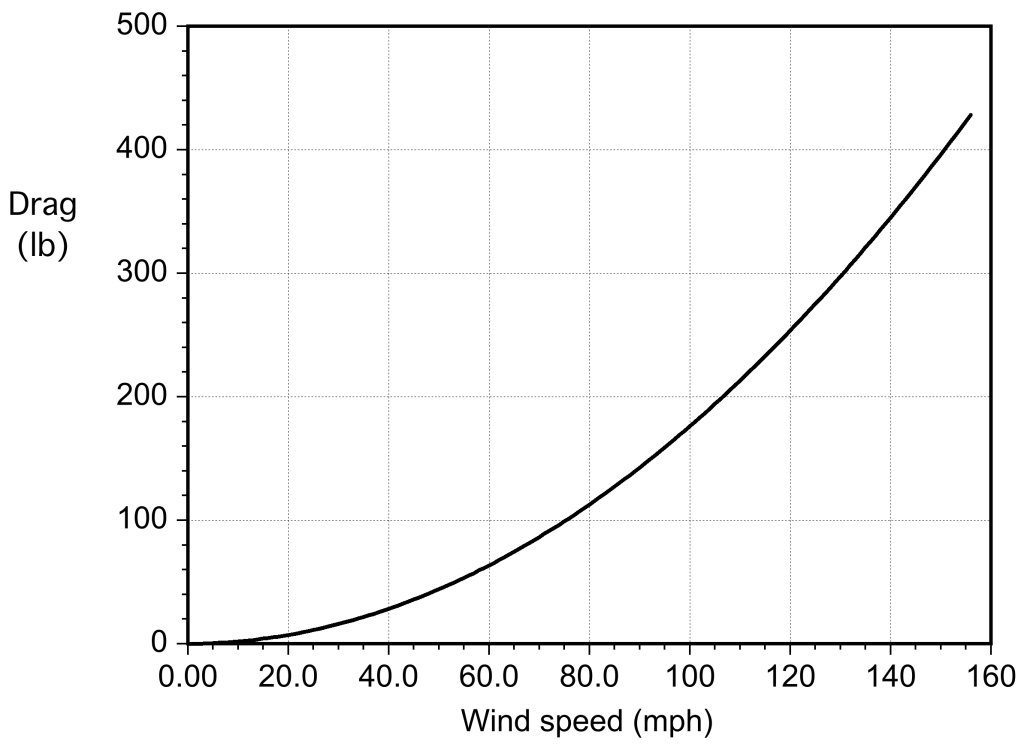
As part of the design of a building structure in Florida, a component is to be tested in a wind tunnel to measure its drag at speeds equivalent to those of a Category 5 hurricane. The component is a bluff body with an estimated drag coefficient of 0.98. The projected cross-sectional area of the component is 3.26 ft ${^{2}}$ . As part of the test plan, the component’s drag force must be estimated before mounting it on the wind-tunnel balance system. Make a plot of the estimated drag force as a function of wind speed up to 156 mph. Assume MSL ISA conditions.

The component is a bluff body with $C_D = 0.98$ and an area $S = 3.26$ ft ${^{2}}$ . The drag $D$ will be

$D = \frac{1}{2} \, \varrho_{\infty} \, V_{\infty}^2 \, S \, C_D$

where $\varrho_{\infty} = 0.002378$ slugs/ft ${^3}$ based on MSL ISA conditions. Therefore,

$D = \frac{1}{2} \times 0.002378 \times \left(1.467 V_{\infty}\right)^2 \times 3.26 \times 0.98 = 0.008175 V_{\infty}^2$

remembering that to convert from mph to ft/s, we must multiply by 1.467. Therefore, it is now a matter of plotting $D$ (in pounds) versus wind speed (in miles per hour) over the specified range using the previous equation, as shown in the plot below.

Worked Example #2

A payload crate is dropped by parachute from a military transport airplane 2,000 m above the ground. The parachute quickly opens, and the crate descends vertically toward the ground. The crate has a mass of 76 kg, a projected cross-sectional area of 0.4 m ${^{2}}$ , and a drag coefficient of 1.5 based on this area. The parachute has an area of 52 m ${^{2}}$ and a drag coefficient of 1.87 based on its projected area. You may assume the average air density during the descent is 1.19 kg/m ${^3}$ . (a) Determine the vertical airspeed at which the crate will parachute to a landing. (b) How long will it take (approximately) for the crate to reach the ground?

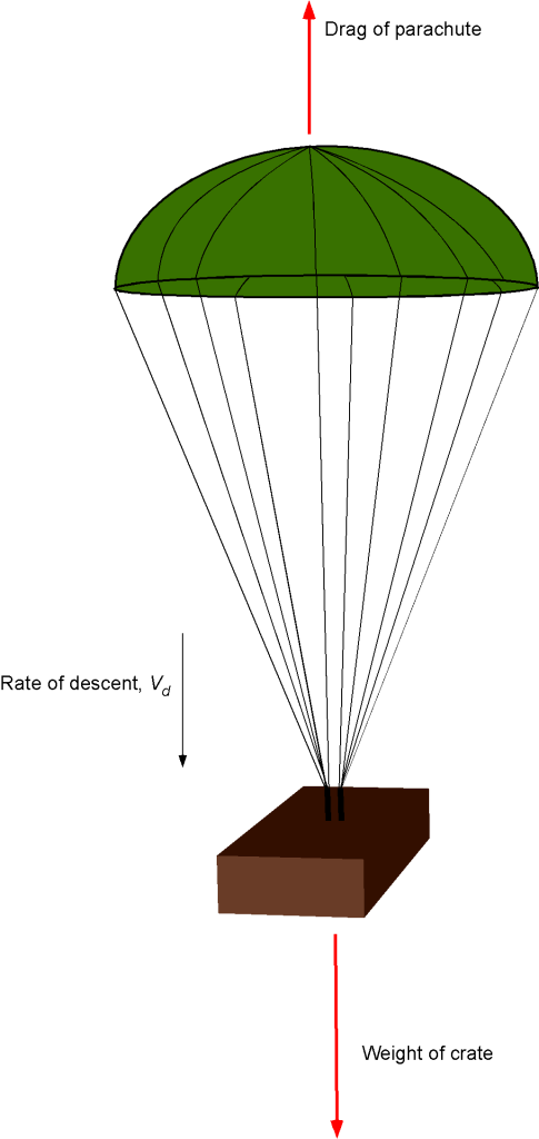
(a) In a steady descent, the net drag will be the sum of the drag produced by the parachute plus the drag of the crate, and this net drag must equal the weight of the crate, i.e.,

$D = W = M \, g = \frac{1}{2} \, \varrho \, V^2 \, S_{\rm body} \, C_{D_{1}} + \frac{1}{2} \, \varrho \, V^2 \, S_{\rm parachute} \, C_{D_{2}}$

where $C_{D_{1}}$ is the drag coefficient of crate and $C_{D_{2}}$ is the drag coefficient of the parachute. We are asked to solve for the vertical airspeed so

$W = M g = \frac{1}{2} \varrho \, V^2 \left( S_{\rm body} \, C_{D_{1}} + S_{\rm parachute} \, C_{D_{2}} \right)$

Rearranging and solving for the airspeed gives

$V = \sqrt{ \frac{2 \, M \, g}{\varrho \left( S_{\rm body} \, C_{D_{1}} + S_{\rm parachute} \, C_{D_{2}} \right) } }$

Inserting the known values gives

$V = \sqrt{ \frac{2 \times 76.0 \times 9.81}{1.19 \times \left( 0.4 \times 1.5 + 52.0 \times 1.87 \right) } } = 3.58~\text{m/s}$

(b) The time $t$ for the descent is found using

$t \approx \frac{2000.0}{3.58} = 559~\text{seconds} = 9.3~\text{minutes}$

Worked Example #3

The wings of older airplanes were often stiffened by wires that provided cross-bracing, as shown in the figure below. Suppose the drag coefficient for the wing is $C_{D_{wing}} = 0.034$ based on the planform wing area ( $S = 180.0$ ft ${^{2}}$ ), determine the ratio of the drag from the wire bracing relative to the drag of the wing when the airplane is flying at 90 mph. Comment on your results. Assume MSL ISA conditions.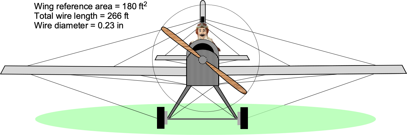

Hint: Obtain the drag coefficient of the wire by using the Reynolds number plot related to a smooth circular cylinder.

The drag of the wing is given by

$D_{\rm wing} = \frac{1}{2} \, \varrho_{\infty} \, V_{\infty}^2 \, S_{\rm wing} \, C_{D_{\rm wing}}$

where $S$ = 180.0 ft ${^{2}}$ and $C_{D_{\rm wing}}$ = 0.034. The drag of the bracing wires is given by

$D_{\rm wire} = \frac{1}{2} \, \varrho_{\infty} \, V_{\infty}^2 \, S_{\rm wire} \, C_{D_{\rm wire}}$

The reference area of the wires is their total projected frontal area, so

$S_{\rm wire} = l \, D = 266.0 \times \left( \dfrac{0.23}{12} \right) = 5.1~\text{ft${^{2}}$}$

where ${l}$ is the total length of the bracing wires, and $D$ is the wire diameter. The determination of the drag of the wires requires the calculation of the Reynolds number of the wire, which is

$Re = \frac{\varrho_{\infty} \,V_{\infty} D}{\mu_{\infty}} = \frac{ 0.002378 \times 90.0 \times 1.467 \times (0.23/12)}{3.737 \times 10^{-7}} \approx 16,100$

noting that 1.467 is the conversion factor from miles per hour (mph) to feet per second (ft/s). From the drag coefficient versus Reynolds number for a circular cylinder, at $Re$ = 16,100, the drag coefficient is about 1.4. Therefore, the total drag of the bracing wires relative to the drag of the wing is

$\frac{D_{\rm wire} }{D_{\rm wing}} = \frac{\frac{1}{2} \, \varrho_{\infty} \, V_{\infty}^2 \, S_{\rm wire} \, C_{D_{\rm wire}}}{\frac{1}{2} \varrho_{\infty} \, V_{\infty}^2 \, S_{\rm wing} \, C_{D_{\rm wing}} } = \frac{S_{\rm wire} \, C_{D_{\rm wire}}}{S_{\rm wing} \, C_{D_{\rm wing}}}$

Inserting the numerical values gives

$\dfrac{D_{\rm wire} }{D_{\rm wing}} = \frac{5.1 \times 1.4}{180.0 \times 0.034} = 1.16$

Notice that the drag of the bracing wire is about the same as that of the unbraced wing. This was a major issue with early externally braced aircraft, significantly limiting their speed. Later, improvements in structural design and stiffer wings led to significant increases in monoplane flight performance.

Notice also that the ratio of the drag values is NOT the ratio of the drag coefficients. This is because the definition of the drag coefficient depends on the reference area. For a wing, the reference area is the planform area; for a wire, the drag coefficient is based on the projected frontal area. Therefore,

$\dfrac{D_{\rm wire} }{D_{\rm wing}} \ne \dfrac{C_{D_{\rm wire}}}{C_{D_{\rm wing}}}$

The ratio of the products of the drag coefficients and the reference areas is

$\dfrac{D_{\rm wire} }{D_{\rm wing}} = \dfrac{S_{\rm wire} \, C_{D_{\rm wire}}}{S_{\rm wing} \, C_{D_{\rm wing}}} = \dfrac{f_{\rm wire}}{f_{\rm wing}}$

where the “ ${\scriptstyle{f}}$ ” values are known as the equivalent drag areas.

Worked Example #4

A general aviation airplane is equipped with a ballistic parachute recovery system for enhanced safety in the event of a severe emergency. Consider a scenario where the airplane’s pilot must deploy this parachute system from an altitude of 3,000 meters. Assume the airplane has a net mass of 1,200 kg, a projected cross-sectional area of 25 m ${^{2}}$ , and a corresponding drag coefficient of 1.8 based on this area. The parachute has an area of 150 m ${^{2}}$ and a drag coefficient of 1.5 based on this area. During the descent, assume an average air density of 1.01 kg \, m ${^{-3}}$ . Disregard the weight of the parachute. Determine the vertical airspeed at which the airplane will parachute to a landing. Approximately how long will the descent take?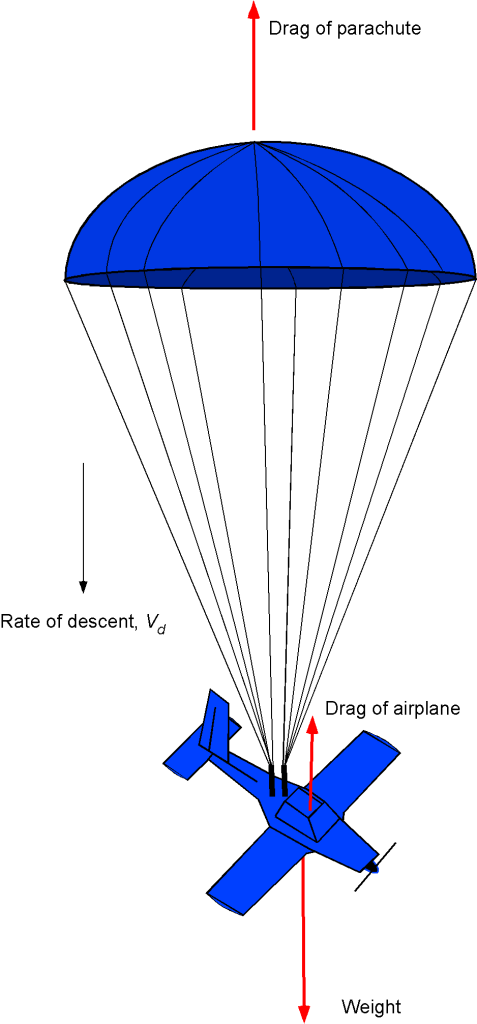

The airplane’s given drag coefficient is two orders of magnitude greater than expected during normal flight. The airplane is streamlined during normal flight, with minimal pressure drag and minimal boundary-layer separation. However, during descent with a parachute, the airplane behaves as a bluff body, with extensive flow separation and corresponding pressure drag. During a steady descent, the net vertical drag on the airplane will equal its weight. The net drag will be the sum of the drag produced by the parachute and the drag of the airplane.

The net drag on the airplane and parachute will be equal to the weight, so

$W = M \, g = \frac{1}{2} \, \varrho \, V_d^2 \, S_a \, C_{D_{a}} + \frac{1}{2} \, \varrho V_d^2 \, S_p \, C_{D_{p}}$

where $V_d$ is the rate of descent, $S_a$ is the projected cross-sectional area of the airplane, $C_{D_{a}}$ is the drag coefficient of the airplane based on this reference, $S_p$ is the projected cross-sectional area of the parachute, $C_{D_{p}}$ is the drag coefficient of the parachute based on this reference area. Simplifying gives

$M \, g = \frac{1}{2} \, \varrho \, V_d^2 \left( S_a \, C_{D_{a}} + S_p \, C_{D_{p}} \right)$

and rearranging to solve for $V_d$ gives

$V_d = \sqrt{ \frac{2 \, M \, g}{\varrho \left(S_a \, C_{D_{a}} + S_p \,C_{D_{p}} \right)}}$

Substituting in the known numerical values gives

$V_d = \sqrt{ \frac{2 \times 1,200.0 \times 9.81 }{1.01 \times \left(25.0 \times 1.8 + 150.0 \times 1.5 \right)} } = 9.29~\text{m/s}$

To compute the descent time $t_d$ , we can assume that the aircraft travels at this vertical speed for the entire change in altitude, so that

$t_d = \frac{h}{V_d} = \frac{3,000}{9.29} = 323~\text{secs} = 5.4~\text{mins}$

Worked Example #5

A re-entry spacecraft weighs 7,000 lb. At an altitude of 2,000 ft, a certain number of parachutes ${N_p}$ (to be determined) must open, each with a diameter ${d}$ of 115 ft as the vehicle descends into the ocean. Based on their projected area, these parachutes have a drag coefficient $C_D$ of 1.6. Assume that after the parachutes are deployed, the spacecraft quickly reaches a descent equilibrium velocity of $V_d$ . During this time, the average air density is $\varrho =$ 0.0023 slug ft ${^{-3}}$ . Ignore drag forces on the spacecraft itself.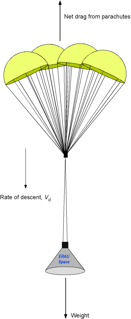

Determine an equation for the spacecraft’s rate of descent with the parachutes open. For example, if the maximum allowable impact speed of the spacecraft with the ocean is 10 ft/s, how many parachutes are required?

During a steady descent, the net vertical drag on the re-entry vehicle from the ${N_p}$ parachutes must equal the vehicle’s weight, i.e., $N_p \, D = W$ , where $D$ is the drag of any one parachute. The aerodynamic drag on any one parachute (a bluff body) will be

$D = \frac{1}{2} \, \varrho \, V_d^2 \, S \, C_{D}$

where $V_d$ is the rate of descent, $S$ is the projected cross-sectional area of any parachute, and $C_D$ is the drag coefficient of the parachute based on this reference area. The net drag on the ${N_p}$ parachutes will be equal to the weight of the vehicle, so the force equilibrium equation is

$W = M \, g = N_p \left( \frac{1}{2} \, \varrho \, V_d^2 \, S \, C_{D} \right) = \frac{1}{2} \varrho \, V_d^2 \, S \, C_{D} \, N_p$

Rearranging to solve for $V_d$ gives

$V_d = \sqrt{ \frac{2 \, M \, g}{\varrho \, S \, C_D \, N_p} }$

which will determine the descent rate for a given number of parachutes.

We are given the maximum allowable rate of descent, so further rearranging the force equilibrium equation to solve for ${N_p}$ gives

$N_p = \frac{ 2 \, W}{\varrho \, V_d^2 \, S \, C_D} = \frac{ 2 \, M \, g}{\varrho \, V_d^2 (\pi \, d^2/4) C_D}$

Substituting in the known numerical values gives

$N_p = \frac{ 2 \times 7,000}{0.0023 \times 10.0^2 \, \pi \times (115.0^2/4.0) \times 1.6} = 3.66$

So, we will need four (4) parachutes to reduce the rate of descent to 10 ft/s.

Worked Example #6

As part of the design of a utility plant in Florida, a solid hemisphere must be tested in a wind tunnel to measure its drag at hurricane speeds. The hemisphere has a diameter of 19 inches. It is to be tested under two conditions: the first with the rounded side into the wind, and the second with the flat side into the wind. As part of the test plan, the drag force on the hemisphere must be estimated before mounting it on the wind-tunnel balance. Make a plot of the estimated drag force on this hemisphere, in both conditions, as a function of wind speed up to 145 mph. You may assume MSL ISA conditions.

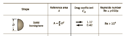
The drag on the hemisphere will be given by the usual formula, i.e.,

$D = \frac{1}{2} \, \varrho \, V^2 \, A_{\rm ref} \, C_D$

where the reference area $A_{\rm ref}$ is

$A_{\rm ref} = \frac{ \pi \, D^2}{4} = \frac{ \pi (19/12)^2}{4} = 1.97~\text{ft${^{2}}$}$

The drag is to be measured in two orientations, the first with the rounded side to the wind, i.e.,

$D_1 = \frac{1}{2} \varrho \, V^2 \, A_{\rm ref} \, C_{D_{1}}$

where according to information given ${C_{D_{1}}}$ = 0.42. In the second case, with the flat side into the wind, then

$D_2 = \frac{1}{2} \, \varrho \, V^2 \, A_{\rm ref} \, C_{D_{2}}$

where $C_{D_{2}} = 1.17$ .

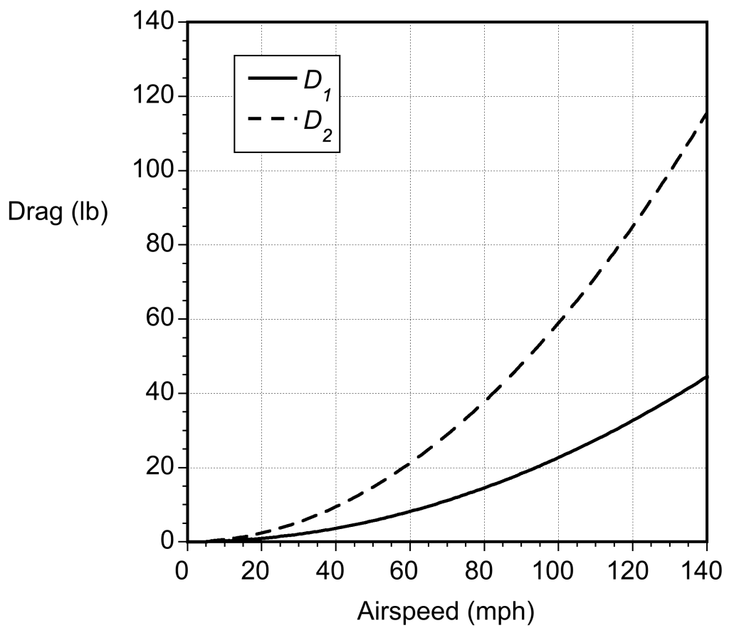
We are told that the airspeed range is up to 145 mph, corresponding to 212.67 ft/s. Therefore, we must plot two curves for $D_1$ and $D_2$ as a function of airspeed. Substituting the numbers and using MSL ISA conditions that $\varrho$ = 0.002378 slugs/ft ${^3}$ gives

$D_1 = \frac{1}{2} \, \varrho \, V^2 \, A_{\rm ref} \, C_{D_{1}} = \frac{1}{2} \times 0.002378 \times 1.97 \times 0.42 V^2 = 0.000984 V^2$

and

$D_2 = \frac{1}{2} \, \varrho \, V^2 \, A_{\rm ref} \, C_{D_{2}} = \frac{1}{2} \times 0.002378 \times 1.97 \times 1.17 V^2 = 0.00274 V^2$

where $V$ would be in units of ft/s. The plot below shows that drag will vary from approximately 45 lb with the rounded side facing the wind to approximately 115 lb with the flat side into the wind. Notice that the wind speed has been converted back to mph for plotting purposes.

Worked Example #7

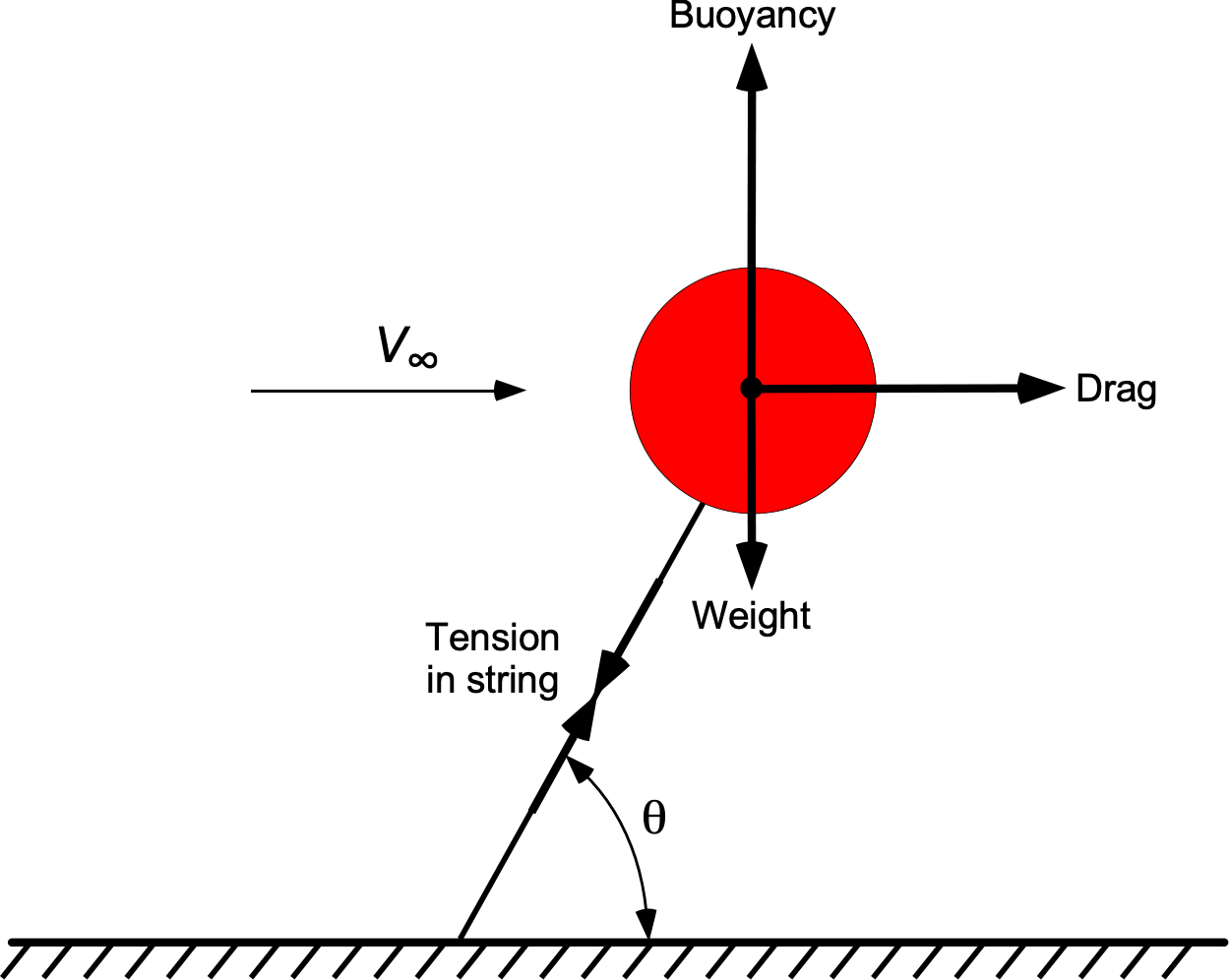
A helium-filled, spherical-shaped balloon with a smooth surface is tethered in a horizontal wind flow of $V_\infty =$ 10.3 mph, as shown in the figure below. The diameter of the balloon is 55 cm, and the mass of the balloon material (not including the gas inside) is 20 grams. The pressure inside the balloon is 120 kPa. Assume MSL ISA atmospheric ambient conditions and for helium $R_{\rm He}$ = 2,077.0 J kg $^{-1}$ K $^{-1}$ .

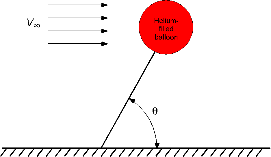
Draw a free-body diagram to show the forces acting on the balloon at its equilibrium condition.
Determine the density of the helium contained inside the balloon at its equilibrium condition.
What is the Reynolds number $Re$ for the flow around the balloon?
Determine the balloon’s drag coefficient, $C_D$ . Hint: Use the chart for $C_D = f (Re)$ for a sphere.
Calculate the value of the equilibrium angle $\theta$ .

The buoyancy force, weight, aerodynamic drag, and tension in the string can be represented in a free-body diagram, as shown below.

2. Using the equation of state, the density of the helium gas in the balloon at 15 $^\circ$ C or 288.15 K is

$\varrho_{He} = \frac{p}{R_{He} \, T} = \frac{120,000}{2,077 \times 288.15} = 0.201~\mbox{kg\,m${^{-3}}$}$

3. The wind speed in base units of m/s is

$V_\infty = 10.3\times 0.447 = 4.60~\mbox{m/s}$

Therefore, the Reynolds number based on the diameter of the balloon and the wind speed is

$Re_{_{D}} = \frac{\varrho_{\rm air} \, V_\infty D}{\mu_{\rm air}} = \frac{1.225 \times 4.60 \times (55.0/100.0)}{1.789 \times 10^{-5}} \approx 173,000$

4. At $Re \approx 173,000$ , the value of $C_D$ is approximately 0.39, per the standard drag chart for a sphere.

5. The projected frontal cross-sectional area of the balloon is

$A = \frac{\pi \, D^2}{4} = \frac{3.14 \times 0.55^2}{4} = 0.2376~\mbox{m${^{2}}$}$

This means that the drag force on the balloon is

$D = \frac{1}{2}\, \varrho_{\rm air} \, V_\infty^2 \, A \, C_D = 0.5 \times 1.225 \times 4.60^2 \times 0.2376 \times 0.39 = 1.20~\mbox{N}$

The volume of the spherical balloon is

${\cal{V}} = \frac{4}{3} \, \pi \left(\frac{D}{2} \right)^3 = 0.0871~\mbox{m${^3}$}$

In the vertical direction, the upward buoyancy force $F_{\rm up}$ and weight $W$ must be considered. The buoyancy force is

$F_{\rm up} = \varrho_{\rm air}\, g \, {\cal{V}} = 1.225 \times 9.81 \times 0.0871 = 1.05~\mbox{N}$

The weight of the balloon, $W_b$ , including the helium gas inside, is

$W = W_{b} + W_{\rm He} = M_{b} \, g + \varrho_{\rm He} \, g \, {\cal{V}}$

Inserting the known numerical values gives

$W = (20.0/1000.0) \times 9.81 + 0.201 \times 9.81 \times 0.0871 = 0.20 + 0.17 = 0.37~\mbox{N}$

Finally, the equilibrium angle $\theta$ is determined from

${ \tan \theta = \frac{F_{\rm up} - W}{D} = \frac{1.05 - 0.37}{1.20} = 0.57 }$

Therefore, $\theta = 29.4^\circ$ .

Worked Example #8

A regulation golf ball has a diameter of 42.67 mm and a mass of 45.9 grams. A golfer drives the ball at 125 mph. Assume MSL ISA atmospheric conditions, i.e., $\varrho_\infty = 1.225$ kg m $^{-3}$ and $\mu_\infty = 1.7894 \times 10^{-5}$ kg m $^{-1}$ s $^{-1}$ .

Determine the Reynolds number for the ball immediately after impact with the club.
Using the appropriate drag chart for a rough sphere or golf ball, estimate a representative value of the drag coefficient, $C_D$ .

1. The launch speed in SI units is $V_0 = 125 \times 0.44704 = 55.88~\mbox{m/s}$ . The Reynolds number based on the ball diameter is

$Re_D = \frac{\varrho_\infty \, V_0 \, D}{\mu_\infty} = \frac{1.225 \times 55.88 \times 0.04267}{1.7894 \times 10^{-5}} = 1.63 \times 10^5$

Therefore, the ball initially flies at a Reynolds number of approximately $1.6 \times 10^5$ .

2. From the standard drag chart for a rough sphere or golf ball, a representative value at this Reynolds number is $C_D \approx$ 0.5. The dimples on a golf ball act as distributed surface roughness and can trip the boundary layer, shifting the drag-crisis behavior to lower Reynolds numbers than for a smooth sphere. The precise value of $C_D$ depends on the ball geometry, spin rate, and Reynolds number, so the value used here should be regarded as an estimate read from the drag chart.

Worked Example #9

A golf ball of diameter 42.67 mm and mass 45.9 grams leaves the clubface with a speed of 50 m/s while spinning with sufficient backspin to produce a lift coefficient of $C_L = 0.18$ . Assume MSL ISA atmospheric conditions, i.e., $\varrho_\infty = 1.225$ kg m $^{-3}$ .

Calculate the lift force on the golf ball.
Compare this lift force with the weight of the ball.
Explain briefly why backspin increases the flight distance of a golf ball.

1. The projected frontal area of the golf ball is

$A = \frac{\pi \, D^2}{4} = \frac{\pi (0.04267)^2}{4} = 1.43 \times 10^{-3}~\mbox{m$^2$}$

The aerodynamic lift force is

$L = \frac{1}{2}\, \varrho_\infty \, V^2 \, A \, C_L = \frac{1}{2} \times 1.225 \times 50.0^2 \times (1.43 \times 10^{-3}) \times 0.18 = 0.394~\mbox{N}$

So the lift force is approximately 0.39 N.

2. The weight of the golf ball is

$W = m \, g = 0.0459 \times 9.81 = 0.450~\mbox{N}$

Therefore,

$\frac{L}{W} = \frac{0.394}{0.450} = 0.876$

and so the lift force is about 88% of the ball’s weight.

3. Because the lift produced by backspin acts upward, which is the Magnus effect, it offsets the weight of the ball, increasing its rate of climb and reducing its rate of descent. Therefore, the ball remains in the air longer, which increases the horizontal distance traveled. This is one of the main reasons why a spinning golf ball flies much farther than a non-spinning ball struck at the same initial speed.

Worked Example #10

A golf ball of mass 45.9 grams and diameter 42.67 mm is struck at 160 mph with a launch angle of 20 $^\circ$ . Assume MSL ISA atmospheric conditions, a representative drag coefficient of $C_D = 0.40$ , and neglect the effects of backspin. Use the approximate equations of motion for quadratic drag acting primarily on the horizontal motion.

Show that the approximate range of the ball may be written as
$R \approx \frac{2 \, m}{\varrho \, A \, C_D}\, \ln\left(1+\frac{\varrho \, A \, C_D \, V_0^2 \sin(2\theta)}{2\, m\, g}\right)$
Calculate the approximate range of the golf ball, and convert the range to yards.

Let the horizontal speed be $u$ . If the drag is assumed to act primarily on the horizontal motion, then

$m\frac{du}{dt} = -\frac{1}{2}\, \varrho \, A \, C_D \, u^2$

Writing

$k = \frac{1}{2}\, \varrho \, A \, C_D$

gives

$m \, \frac{du}{dt} = -k \, u^2$

If the initial horizontal speed is

$u_0 = V_0 \, \cos\theta$

then integration gives

$u(t) = \frac{u_0}{1 + \dfrac{k \, u_0}{m} t}$

Integrating once more, the horizontal distance is

$x(t) = \frac{m}{k}\ln\left(1+\frac{k \, u_0}{m}t\right)$

If the vertical motion is assumed to remain approximately ballistic, then the time of flight is

$t_f \approx \frac{2\, V_0\sin\theta}{g}$

Substituting $u_0 = V_0 \, \cos\theta$ and $t = t_f$ gives

$R \approx \frac{m}{k}\ln\left(1+\frac{k \, V_0^2\, \sin(2\theta)}{m\, g}\right)$

and because $k = \dfrac{1}{2} \, \varrho \, A \, C_D$ , then

$R \approx \frac{2\, m}{\varrho \, A \, C_D}\, \ln\left(1+\frac{\varrho \, A \, C_D \, V_0^2 \sin(2\theta)}{2 \, m\, g}\right)$

as required.

2. The launch speed is $V_0 = 160 \times 0.44704 = 71.53~\mbox{m/s}$ . The projected frontal area of the golf ball is

$A = \frac{\pi \, D^2}{4} = \frac{\pi (0.04267)^2}{4} = 1.43 \times 10^{-3}~\mbox{m$^2$}$

Therefore,

$R \approx \frac{2 \times 0.0459}{1.225 \times (1.43\times10^{-3}) \times 0.40} \ln\left(1+\frac{1.225 \times 1.43\times10^{-3} \times 0.40 \times (71.53)^2 \times \sin 40^\circ}{2 \times 0.0459 \times 9.81}\right) \approx 166~\mbox{m}$

Converting to yards gives $R = 166 \times 1.094 = 182 \mbox{yd}.$ Therefore, the approximate range of the golf ball is about 166 m, or approximately 182 yards. Because backspin has been neglected, an actual well-struck golf shot would generally travel farther than this value.

Worked Example #11

A golf ball of diameter 42.67 mm and mass 45.9 grams is struck with a speed of 60 m/s and a backspin rate of 3,000 rpm. Assume MSL ISA atmospheric conditions, i.e., $\varrho_\infty = 1.225$ kg m $^{-3}$ . A reasonable approximation for the lift coefficient of a spinning sphere is

$C_L \approx 1.6 \, S$

where the spin parameter is

$S = \frac{\omega \, R}{V}$

Here, $\omega$ is the angular velocity in rad/s, $R$ is the radius of the ball, and $V$ is the translational speed.

Determine the spin parameter, $S$ .
Estimate the lift coefficient, $C_L$ .
Calculate the lift force acting on the golf ball.
Compare the lift force with the weight of the ball.

1. The angular velocity corresponding to 3,000 rpm is

$\omega = 3,000 \times \frac{2\pi}{60} = 314.16~\mbox{rad/s}$

The radius of the ball is

$R = \frac{D}{2} = \frac{0.04267}{2} = 0.02134~\mbox{m}$

Therefore, the spin parameter is

$S = \frac{\omega \, R}{V} = \frac{314.16 \times 0.02134}{60.0} = 0.112$

2. The lift coefficient is approximated by

$C_L \approx 1.6 \, S = 1.6 \times 0.112 = 0.179 \approx 0.18$

3. The projected frontal area of the golf ball is

$A = \frac{\pi \, D^2}{4} = 1.43 \times 10^{-3}~\mbox{m$^2$}$

The lift force is

$L = \frac{1}{2}\, \varrho_\infty \, V^2 \, A \, C_L = \frac{1}{2} \times 1.225 \times 60.0^2 \times (1.43 \times 10^{-3}) \times 0.18 = 0.56~\mbox{N}$

4. The weight of the golf ball is

$W = m \, g = 0.0459 \times 9.81 = 0.450~\mbox{N}$

Therefore,

$\frac{L}{W} = \frac{0.56}{0.45} \approx 1.24$

So the lift force exceeds the ball’s weight. This result shows that the Magnus effect can produce a lift force comparable to or greater than the golf ball’s weight, thereby significantly increasing its time of flight and, consequently, its range.

Worked Example #12

A box-shaped delivery truck is traveling at a speed of 65 mph on a highway. The frontal area of the truck is 8.0 m $^2$ , and its length is 8.0 m. Assume MSL ISA atmospheric conditions, i.e., $\varrho_\infty = 1.225$ kg m $^{-3}$ and $\mu_\infty = 1.7894 \times 10^{-5}$ kg m $^{-1}$ s $^{-1}$ .

Determine the Reynolds number for the flow around the truck.
Estimate a representative drag coefficient, $C_D$ , for the truck.
Calculate the aerodynamic drag force acting on the truck.
Determine the power required to overcome this drag.

1. The velocity in SI units is $V = 65 \times 0.44704 = 29.06~\mbox{m/s}$ . The Reynolds number based on the length of the truck is

$Re_L = \frac{\varrho_\infty \, V \, L}{\mu_\infty}$

so that

$Re_L = \frac{1.225 \times 29.06 \times 8.0}{1.7894 \times 10^{-5}} = 1.59 \times 10^7$

Therefore, the flow is fully turbulent.

2. A box-shaped truck is a classic angular bluff body with large-scale flow separation, almost independent of Reynolds number. A representative drag coefficient for this shape is $C_D \approx 1.0$ .

3. The drag force is

$D = \frac{1}{2}\, \varrho_\infty \, V^2 \, A \, C_D = \frac{1}{2} \times 1.225 \times 29.06^2\times 8.0 \times 1.0 = 4.13 \times 10^3~\mbox{N}$

4. The power required to overcome this drag is

$P = D \, V = (4.13 \times 10^3) \times 29.06 = 1.20 \times 10^5~\mbox{W} \approx 120~\mbox{kW}$

Worked Example #13

A team of AIAA DBF students is required to design a banner to be towed behind a small electric airplane. The banner must have a fixed aspect ratio of $AR=5$ , but maximum points are awarded for the largest possible banner. Assume the airplane tows the banner at a speed of 20 m\,s $^{-1}$ at MSL ISA conditions, i.e., $\varrho_\infty = 1.225$ kg m $^{-3}$ . The airplane can supply at most 150 W of additional power to tow the banner.

Write down the relationship between the drag of the banner and the towing power.
Determine an estimate for the maximum allowable banner area and corresponding banner dimensions.

1. The drag force on the banner is

$D = \frac{1}{2}\,\varrho_\infty \, V_\infty^2 \, A \, C_D$

and the additional power required to tow the banner is $\Delta P = D\, V_\infty$ . Therefore,

$\Delta P = \frac{1}{2}\,\varrho_\infty \, V_\infty^3 \, A \, C_D$

2. Based on wind tunnel tests of banners, for which results are given in the main text, a practical design estimate for a banner of aspect ratio 5 is $C_D \approx 0.20$ , which will be used in the remainder of the problem. Solving for the banner area gives

$A = \frac{2 \, \Delta P}{\varrho_\infty \, V_\infty^3 \, C_D}$

so that in this case

$A = \frac{2 \times 150}{1.225 \times 20^3 \times 0.20} = 0.153~\mathrm{m}^2$

The aspect ratio is $AR = \dfrac{l}{w} = 5$ and the area is $A = l\,w$ . Because $l = 5w$ , then $A = 5w^2$ , so that

$w = \sqrt{\frac{A}{5}} = \sqrt{\frac{0.153}{5}} = 0.175~\mathrm{m}$

and $l = 5w = 0.875~\mathrm{m}.$ Therefore, the DBF team will want to use a banner of dimensions $w \approx$ 0.18 m and $l \approx$ 0.88 m. Flight testing will determine whether these estimates are valid.

Worked Example #14

A general aviation airplane of weight 2,020 lb with a lift-to-drag ratio of 10 has a fixed tricycle undercarriage consisting of two main wheels and one nose wheel. Each main wheel has a diameter of 18 in and a width of 6 in, and the nose wheel has a diameter of 14 in and a width of 5 in. The airplane cruises at 120 mph at MSL ISA conditions. Assume that the wheels may be treated as bluff bodies based on their projected frontal area, and that the drag coefficient of each exposed wheel is $C_D = 0.40$ . If the wheels are fitted with streamlined wheel spats, assume that the corresponding drag coefficient becomes $C_D = 0.08$ .

Estimate the total drag of the wheels when they are fully exposed to the flow.
Estimate the total drag when the wheels are fitted with wheel spats.
Determine the drag reduction produced by the wheel spats.
Estimate the corresponding reduction in power required at the cruise speed.
Estimate the new cruise speed when wheel spats are installed, assuming that the available power remains the same.

1. For a bluff body, the drag is

$D = \frac{1}{2}\,\varrho_{\infty}\,V_{\infty}^{2}\,C_D\,S$

where $\varrho_{\infty} = 0.002378$ slugs/ft $^3$ at MSL ISA conditions. The cruise speed is

$V_{\infty} = 120 \times 1.467 = 176.0 \;\mathrm{ft/s}$

The projected area of each main wheel is

$S_m = d_m \, w_m = 1.5 \times 0.5 = 0.75 \;\mathrm{ft}^2$

because 18 in = 1.5 ft and 6 in = 0.5 ft. Therefore, the projected area of the two main wheels is

$2S_m = 1.50 \;\mathrm{ft}^2$

The projected area of the nose wheel is

$S_n = d_n w_n = 1.167 \times 0.417 = 0.487 \;\mathrm{ft}^2$

because 14 in = 1.167 ft and 5 in = 0.417 ft. Hence, the total projected area of the three wheels is

$S_{\mathrm{tot}} = 1.50 + 0.486 = 1.987 \;\mathrm{ft}^2$

For the exposed wheels, using $C_D = 0.40$ ,

$D_{\mathrm{exp}} = \frac{1}{2} \times 0.002378 \times (176.0)^2 \times 0.40 \times 1.986$

which gives

$D_{\mathrm{exp}} = 29.3 \;\mathrm{lb}$

2. For the wheels fitted with spats, using $C_D = 0.08$ , then

$D_{\mathrm{spat}} = \frac{1}{2}\times 0.002378 \times (176.0)^2 \times 0.08 \times 1.986 = 5.86 \;\mathrm{lb}$

3. Therefore, the drag reduction produced by the wheel spats is

$\Delta D = D_{\mathrm{exp}} - D_{\mathrm{spat}} = 29.3 - 5.86 = 23.4 \;\mathrm{lb}$

4. The power associated with this drag reduction is

$\Delta P = \Delta D\,V_{\infty} = 23.4 \times 176.0 = 4118 \;\mathrm{ft\, lb/s}$

Because 1 hp = 550 ft lb/s, then

$\Delta P = \frac{4118}{550} = 7.49 \;\mathrm{hp}$

5. Notice that the total airplane drag at 120 mph with exposed wheels will be $W/(L/D)$ = 2,020/10 = $D_{\mathrm{tot,exp}} =$ 202 lb. With wheel spats installed, the total drag at the same speed becomes $D_{\mathrm{tot,spat}} = 202 - 23.4 = 178.6 \;\mathrm{lb}$ . Assuming the available power remains the same and that the change is primarily in parasite drag, then $P \propto V^3$ , so that

$\frac{V_{\mathrm{spat}}}{V_{\mathrm{exp}}} = \left(\frac{D_{\mathrm{tot,exp}}}{D_{\mathrm{tot,spat}}}\right)^{1/3}$

Therefore,

$V_{\mathrm{spat}} = 120\left(\frac{202}{178.6}\right)^{1/3}$

which gives $V_{\mathrm{spat}} = 125.0 \;\mathrm{mph}$ . Hence, the use of wheel spats increases the cruise speed by approximately $\Delta V = 125.0 - 120.0 = 5.0 \;\mathrm{mph}$ . This result shows that although the wheel spats affect only a small part of the airplane, they can produce a worthwhile reduction in parasite drag, reduce the power required by about 7.5 hp at cruise, and increase the cruise speed by about 5 mph.

Worked Example #15

A simple 3-cup anemometer consists of three identical hemispherical cups mounted on arms of length $R$ , where $R$ is the distance from the axis of rotation to the center of each cup. Each cup has a projected frontal area $A$ . The wind has a freestream speed ${V_{\infty}}$ , and the cups rotate with angular velocity $\Omega$ . Let $\psi$ denote the azimuth angle of a cup measured from the upstream wind direction. The air density is $\varrho_{\infty}$ . Assume that the drag coefficient of a hemispherical cup depends on its orientation to the flow: it is $C_{D,c}$ when the concave side faces the wind and $C_{D,v}$ when the convex side faces the wind. Assume negligible bearing friction, negligible arm drag, no aerodynamic interference between cups, and steady rotation.

(a) Explain why the anemometer rotates, and develop an expression for the mean aerodynamic torque over one complete revolution.

(b) Using $C_{D,c} = 1.17$ and $C_{D,v} = 0.42$ , find an expression for the wind speed in terms of the rotational speed of the anemometer by imposing the steady-state condition that the mean aerodynamic torque over one revolution is zero.

(a) A cup anemometer rotates because a hemispherical cup has a larger drag coefficient when its concave side faces the wind than when its convex side faces the wind. This drag difference produces a net aerodynamic torque. For a cup at azimuth angle $\psi$ , the tangential component of the relative wind is

$V_t = \Omega \, R + V_{\infty}\, \sin\psi$

and the relative speed as

$V_{\rm rel} = \left( (\Omega \, R)^2+V_{\infty}^2 + 2\Omega \, R \, V_{\infty}\sin\psi \right)^{1/2}$

The instantaneous torque from one cup is

$Q(\psi) = -\frac{1}{2} \, \varrho_{\infty} \,A \,R \,C_D(\psi)\,V_{\rm rel}\,V_t$

so the mean torque from the three cups is

$\overline{Q} = -\frac{3}{2}\,\varrho_{\infty} \,A \,R \, \frac{1}{2\pi} \int_0^{2\pi} C_D(\psi) \left( (\Omega \,R)^2 + V_{\infty}^2 + 2\Omega \, R \, V_{\infty}\, \sin\psi \right)^{1/2} \left(\Omega \,R + V_{\infty}\, \sin\psi\right) \,d\psi$

(b) The drag from the cups can be expressed as

$C_D(\psi) = \overline{C_D} - \frac{\Delta C_D}{2}\sin\psi$

where

$\overline{C_D} = \frac{1.17+0.42}{2} = 0.795$

and

$\Delta C_D = 1.17 - 0.42 = 0.75$

Therefore,

$C_D(\psi) = 0.795 - 0.375\sin\psi$

Then the steady-state condition $\overline{Q}=0$ becomes

$\int_0^{2\pi} \left(0.795-0.375\sin\psi\right) \left(1+\mu^2+2\,\mu\, \sin\psi\right)^{1/2} \left(\mu + \sin\psi\right) \,d\psi =0$

where $\mu=\dfrac{\Omega \, R}{V_{\infty}}$ . Numerical solution gives $\mu=\dfrac{\Omega R}{V_{\infty}}\approx 0.16$ , so $\Omega R \approx 0.16 V_{\infty}$ and $\Omega \approx \dfrac{0.16 V_{\infty}}{R}$ .

License

Icon for the Creative Commons Attribution-NonCommercial-NoDerivatives 4.0 International License

Introduction to Aerospace Flight Vehicles Copyright © 2022–2026 by J. Gordon Leishman is licensed under a Creative Commons Attribution-NonCommercial-NoDerivatives 4.0 International License, except where otherwise noted.

Digital Object Identifier (DOI)

https://doi.org/https://doi.org/10.15394/eaglepub.2022.1066.9

License

Digital Object Identifier (DOI)

Share This Book