Introduction

Fluid dynamics is a discipline of engineering that describes the behavior of moving fluids, i.e., the mechanism of how fluids flow from one place to another. Fluids can be either liquids or gases. Of particular interest to aerospace engineers is the field of aerodynamics, which is the study of airflow. In general, gas dynamics (or gasdynamics) is the study of the flow of gases other than air. Hydrodynamics is the study of liquids in motion, although the name hydrodynamics may be applied to fluids in a broader context.

The solution to fluid dynamic problems usually involves predicting or measuring the properties of the fluid, such as its flow velocity, pressure, density, temperature, viscosity, etc. These properties are called macroscopic fluid properties because they apply to a sizeable finite group of molecules of measurable dimensions, i.e., under the assumption of a continuum. The term “measurable dimensions” can be considered equivalent to the diameter of the tip of one’s pen or pencil, about 0.5 mm or 0.02 (twenty thousandths) of an inch. Such fluid properties may be functions of the position (i.e., what is called spatial location) and, perhaps, of time (i.e., an unsteady flow). However, as a primer to understanding and predicting aerodynamic flows, it is first necessary to define the types of fluid flows encountered in engineering practice, including laminar versus turbulent flows, steady versus unsteady flows, and incompressible versus compressible flows.

Laminar & Turbulent Flows

Fluid flows can be classified into two primary types: laminar and turbulent. There is no mixing between fluid layers in a laminar flow; they move smoothly in layers or laminas. Laminar flows, however, transition naturally after some time (or some downstream flow distance) and become turbulent; such behavior is inevitable and predictable, at least in a naturally occurring flow environment. In a turbulent flow, the fluid layers mix, and the action of viscosity creates internal shear stresses that result in the formation of spinning fluid elements and the creation of eddies and turbulence, as shown in the flow visualization image below.

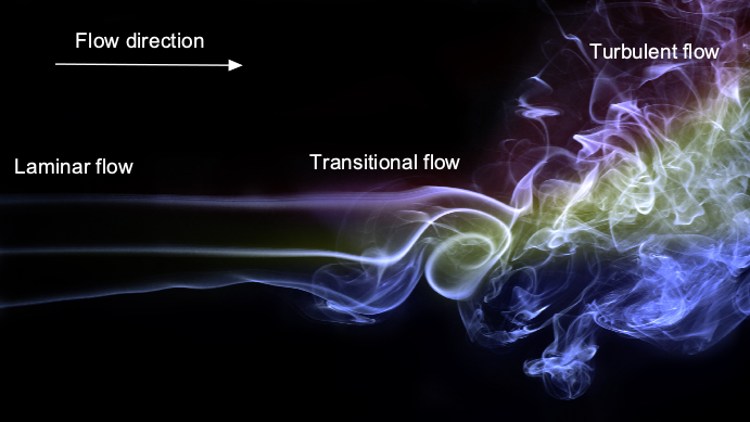
Turbulent flows are the most common flows encountered in practice, but laminar flows can exist under some specific circumstances, at least briefly after the flow is first formed. The third flow type can be classified as a transitional flow in that this flow is neither completely laminar nor thoroughly turbulent. Laminar flows will “transition” through this state before becoming fully turbulent, which is a process, not a sudden event, hence the name.

Consider now a classic flow experiment to examine the difference between laminar and turbulent flows, an investigation first conducted by Osborne Reynolds, where a dye was ejected into a pipe flow, as illustrated in the figure below. Reynolds found that it exited in a smooth or laminar flow form when the dye was introduced at low speeds. However, after a short distance, the flow naturally started to mix between the fluid layers, and then, after some further distance, the flow became more fully mixed. This mixed flow is called a turbulent flow, which is filled with random turbulent eddies of various sizes and intensities. Reynolds noted that the higher the flow velocity, the quicker the flow transitioned to a turbulent flow – see here for flow visualization of the process. He also determined that the process depended on the properties of the fluid, specifically its density and viscosity.

Turbulent flows are not easy to describe from the perspective of measurement or calculation, and statistical methods must be used. A turbulent flow is often called stochastic or non-deterministic because of its random nature. The formal concept of a stochastic process is classically called a random process. Osborne Reynolds found that this behavior was related to the flow velocity, the type of fluid in the pipe, as well as the diameter of the pipe. He obtained a non-dimensional parameter involving the flow velocity, , its density, , dynamic viscosity, , and the pipe diameter, , now known as the Reynolds number. The Reynolds number is given the symbol , and the equation is

(1)  

In general, the Reynolds number is defined as

(2)  

where is a characteristic length scale for that flow.

The numerical value of the Reynolds number is used as a measure of the relative significance of viscous effects in a fluid. For Reynolds numbers of less than 2,000, then flows are generally laminar. When the Reynolds number exceeds about 4,000 to 5,000, the flow transitions from its laminar state and becomes turbulent. The transition from laminar to turbulent flow is not a fixed point but a process, and so it occurs in the range of Reynolds numbers between these values. External influences may influence the transition Reynolds number range – upstream turbulence or external pressure disturbances tend to lower the Reynolds number at which transition occurs.

Ideal Flow

A fluid that is not subjected to the action of viscosity or compressibility and does not flow in a turbulent manner is called an ideal or inviscid fluid. Further qualifications for an ideal (or perfect) fluid include no surface tension effects, and if a liquid, it does not vaporize. In general, an ideal fluid flow has no internal dissipation of energy or other losses associated with the effects of viscosity and turbulence. In reality, no fluid can ever really be entirely ideal. However, under some circumstances, fluid behavior approaches the ideal, for which the analysis is much easier than if the flow was considered viscous and turbulent. Such ideal flows are often referred to as potential flows, for which a large body of technical literature exists. Such potential flows are also used as exemplars for those learning fluid dynamics.

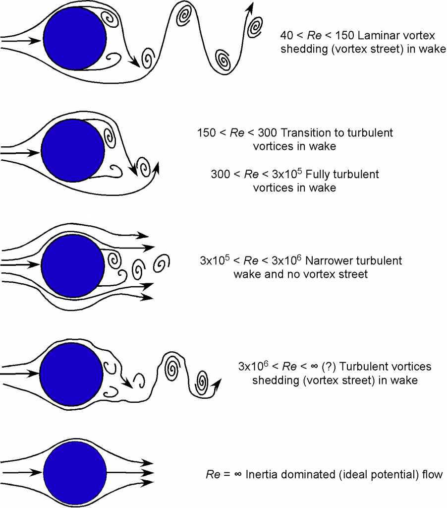
For example, the figure below shows the diversity of different flow patterns obtained to varying values of the Reynolds number, which measures the relative effects of inertia to viscous effects. At low values of , the inertia in the flow is flow, so the effects of viscosity are more important. In this case, the flow experiences flow separation and the formation of swirling flows called vortices and turbulence. In the limiting case, when , the inertia effects in the flow dominate over viscous effects, and the flow approaches an ideal flow, free of vortices and turbulence. The further implications of the Reynolds number parameter on fluid flows are considered later.

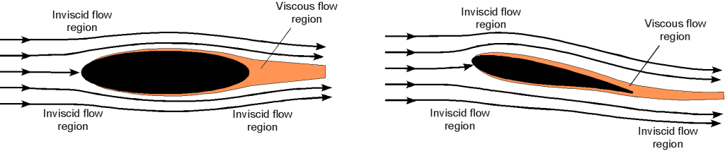
Because turbulence makes problem-solving in fluids much more difficult, it is often convenient to divide real fluid flows into different flow regions or zones, which may be considered either predominantly ideal and inviscid or predominantly viscous and turbulent. Such a division or zonal decomposition is often used to analyze aerodynamic problems, primarily when the regions with a turbulent flow are confined to small parts of the entire flow field, as shown in the figure below. The near-wall flows over surfaces or around bodies are inevitably viscous-dominated because of the shearing effects produced in the flow. The critical part of this decomposition approach is how the regions (zones) are coupled computationally, i.e., how information is passed between the zones. A flow simulation with a zonal method costs more (computationally) than one for an entirely inviscid solution. However, it is still generally much less time-consuming than a full viscous simulation.

Steady Versus Unsteady Flows

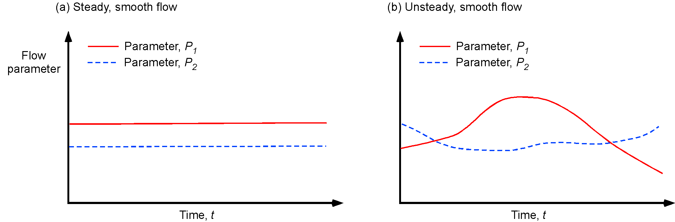
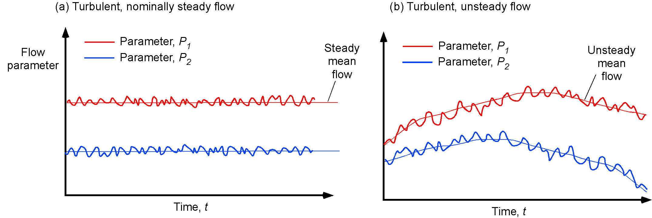
A flow with properties that do not change as a function of time is called a steady flow. A steady-state flow refers to the condition where the macroscopic flow properties, such as the velocity and pressure at a point, do not change with respect to time, as shown in the figure below on the left. However, in a time-dependent flow, also known as an unsteady flow, the flow properties at a point will change with time, as shown in the figure below on the right. Mathematically, for steady flows, then

(3)  

where is any fluid property such as pressure, temperature, velocity, density, etc.

Unsteady flow phenomena are encountered in many engineering applications. Examples include the flows in turbomachinery and piston engines, helicopter aerodynamics, and aeroacoustics. A turbulent flow is an unsteady flow, by definition. However, a turbulent flow can be statistically steady. This definition means that the average flow velocity and other quantities are constant with respect to time, and all the statistically varying properties, such as the component of the fluctuating velocity, are constant with respect to time.

One reason it is helpful to distinguish between steady and unsteady flows is that the former is often more tractable to understand, as well as to predict. To this end, eliminating time from the solution of the equations that govern a fluid flow problem usually results in a significant simplification of the relevant governing equations as well as the mathematical and/or numerical techniques needed to solve these equations.

Reynolds Decomposition

The figure below shows the difference between a statistically steady mean turbulent flow and a statistically unsteady flow. A flow property can be decomposed into a mean or average part, , and a statistically mean fluctuating part, , i.e.,

(4)  

Notice that and are functions of time and space, but the averages is a function of space only. This process has a particular name, which is called a Reynolds decomposition. Reynolds decomposition can also be extended to three dimensions, where each quantity can be separately decomposed into its mean and fluctuating components.

The mean values can be obtained by averaging the flow properties over a long period, say , so that for a given spatial location in the flow, say , then

(5)  

How long needs to be to obtain the desired information depends on the flow. The general rule is that must be long enough for statistical convergence, which often means as long as practically possible within the times and constraints of any experiment. Formal convergence studies may also need to be performed so that the results are within accepted statistical bounds.

Therefore, the turbulent part is

(6)  

from which the root mean square (rms) or “strength” of the turbulent flow can be defined as

(7)  

In practice, these averaged values are found from discrete values (i.e., flow measurements made at discrete time intervals), so summations replace the integrals. For a discretely sampled time-history of values, then performing Reynolds decomposition gives the mean component as

(8)  

where is the number of contiguous measurements. To ensure validity, the value of must be sufficiently large that statistical convergence is obtained, typically needing thousands of samples.

Reduced Frequency

One important parameter used to help categorize whether a flow is steady or unsteady is the reduced frequency, given the symbols, , and defined as

(9)  

where is a characteristic physical frequency of the unsteady flow, is a characteristic length scale, and is a reference flow velocity. For a wing or airfoil, the reduced frequency is normally defined in terms of its semi-chord, i.e., , and the free-stream velocity.

For = 0, the flow is steady. For 0 0.05, the flow can be considered quasi-steady; that is, unsteady effects are generally minor, and for some problems, they may be neglected completely. However, such bounds are subjective and not based on rigorous analysis. In quasi-steady flows, the behavior can be evaluated by applying the principles of steady flow under the instantaneous boundary conditions, i.e., it is assumed that flow adjustments take place instantaneously.

Flows with characteristic reduced frequencies of 0.05 and above are generally considered unsteady, so the flow physics begins to change, and quasi-steady assumptions become invalid. Problems with characteristic reduced frequencies of 0.2 and above are considered highly unsteady, and the unsteady effects will begin to dominate the flow characteristics. Such problems are much more difficult to determine because the local flow properties also depend on the previous time, i.e., what has happened in the time history of the lift and other aerodynamic forces.

Compressible Versus Incompressible Flows

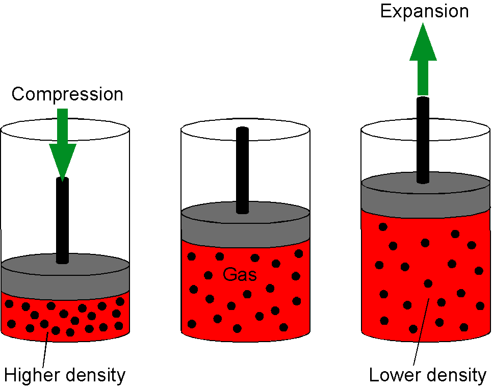
The term “compressibility” applied to a fluid means that a fluid can be compressed, squeezing the fluid and bringing the molecules closer together. Gases are easily compressed because the molecules are relatively far apart, but liquids are incompressible. The volume and density of a gas can be easily changed by changing its pressure or by changing the volume, thereby changing the density, e.g., by squeezing it or otherwise compressing it.

In this regard, consider a simple experiment with a gas in a sealed cylinder, as shown in the figure below. As the piston moves downward and decreases the volume and the pressure, the gas is compressed, and the molecules are now closer together, i.e., the density of the gas increases, and more molecules impact over a smaller area of the cylinder. Because work is also done on the gas to compress it, its temperature will also increase. Similarly, if the piston moves upward, the volume and pressure decrease, so the gas density and temperature both decrease. Therefore, it can be concluded that a gas flow in which the density, , varies in either space and/or time is called a compressible flow. In contrast, a flow where the density is constant everywhere is called an incompressible flow.

All gas flows are compressible to a lesser or greater degree. However, many gas-dynamic and aerodynamic problems can be modeled as incompressible without significant accuracy loss. This distinction is important because solving problems involving compressibility effects is generally much more complicated than those classified as incompressible.

Gases are always compressible because they have molecules that are relatively far apart, so there is plenty of space to squeeze them closer together. Therefore, the density of gases changes readily with even modest changes in temperature and pressure. In a gas, the density is related to temperature and pressure by the ideal gas law, given by . The change in pressure in a fluid, , may be written as

(10)  

where is the bulk compression modulus of the particular fluid. The minus sign indicates that a decrease in volume accompanies increased pressure. The bulk compression modulus is a material property characterizing the compressibility of the gas, i.e., how easily a unit volume of a gas can be changed when changing the pressure acting upon it. Furthermore, the speed of sound can be calculated from the bulk modulus and the fluid density using

(11)  

Liquids, however, are difficult to compress because the molecules are closer together (but they are still very mobile), and for most problems, liquids may be considered entirely incompressible. It is necessary to consider the physics of compressibility in liquids only when sound propagation effects need to be considered. For a liquid, the density is related to temperature as a coefficient of expansion, just as in a solid.

Under flow conditions that involve only slight changes in velocity or pressure, even gases may be considered incompressible. This assumption is usually appropriate for low-speed flow or what might be called low subsonic flows, i.e., flows where the flow velocities are much less than the speed of sound. However, the flow must always be considered compressible for flows at higher subsonic speeds, especially those involving shock waves.

Mach Number Effects

The Mach number is often used to measure the significance of compressibility effects. The study of compressible flows is relevant to problems associated with high-speed aircraft, jet engines, rocket engines, rockets, spacecraft exiting and re-entering the atmosphere, etc. The figure below schematically shows the flow about a wing’s cross-section; the free-stream Mach number varies from low subsonic to supersonic. It is apparent that the effects of the Mach number are significant, and the flow patterns about the wing change significantly.

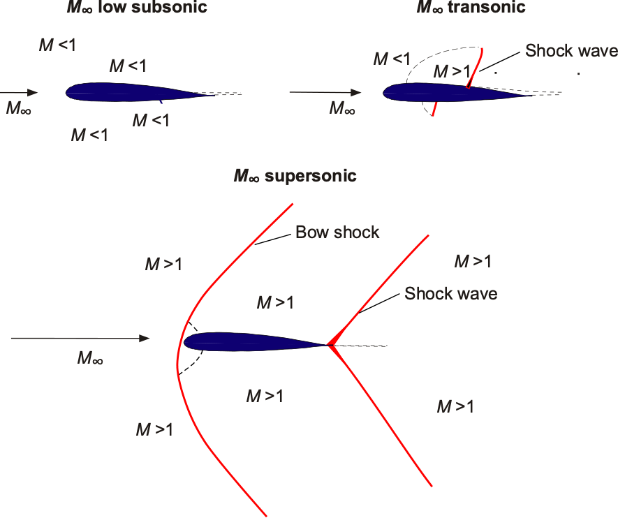
It should be clear why the Mach number can be used to measure compressibility effects in a flow. First, however, it is essential to note that the free-stream Mach number by itself is not a reliable indicator of whether the local flow can be considered incompressible. This is because as the flow approaches and passes around a body, such as an airfoil, it will be locally accelerated, and its local velocity (particularly near its leading edge or nose) will increase. For example, suppose the free-stream Mach number is 0.3. As the flow accelerates over the upper surface of an airfoil, the local Mach number may be as high as 0.5 or 0.6, or even higher, depending on the airfoil’s angle of attack.

However, the flow may be treated as essentially incompressible for flows around wings and bodies where the local value of is less than about 0.3. To verify this, consider a fluid element initially at rest, which has density . If this flow is accelerated to some velocity and some Mach number , the density of the fluid can be assumed to change according to the isentropic relationship

(12)  

where for air, the result in Eq. 12 being plotted in the figure below.

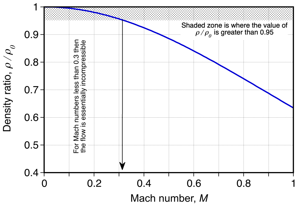
Notice that the variation of from unity is negligible at low Mach numbers. Therefore, for local Mach numbers below a threshold of about 0.3, i.e., the density varies less than 5% for , the flow can usually be treated as incompressible, and it is convenient to make this simplifying assumption in flow analysis. However, this incompressible flow assumption cannot be easily made for higher Mach numbers without introducing significant errors in predicting the flow properties. Therefore, in the case of compressible flows, the thermodynamic equation of state must be used to relate the flow properties.

The corresponding isentropic flow equations for pressure and temperature are also helpful to consider. For the pressure ratio, then

(13)  

and for the temperature

(14)  

Another critical difference between incompressible and compressible flows is because of temperature changes. For an incompressible flow, any temperature changes are generally small. However, in a compressible flow, significant temperature changes may occur. The threshold is that if , the flow can usually be treated as incompressible.

Swirling Vortex Flows

Vortex flows are characterized by swirling motion, where fluid rotates around a central axis and forms cylindrical shapes. They can be found in many natural phenomena, such as hurricanes, tornadoes, whirlpools, and wingtip vortices from airplanes and other flight vehicles. The formation of vortices is complicated and depends on many factors, including changes in fluid velocity, pressure gradients, and the presence of boundaries.

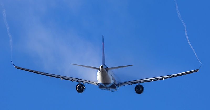
Aeronautical engineers are particularly interested in wing tip vortices, which are the vortices formed and trailed in the wake behind the wingtips of an aircraft as it flies. These vortices are created from the difference in pressure between the upper and lower surfaces of the wing, which creates a tightly swirling flow of air that rotates around the wing tip. Wing tip vortices can also be a significant source of drag on the aircraft, which is called “induced drag.” If the aircraft has a winglet, as shown in the photograph below, the vortex typically trails from the tip of the winglet. Besides the drag caused by the wingtip vortices, they can also pose a hazard to following aircraft, which may get caught up in the wake and may experience a wake-induced upset.

Vortex flows can also be studied in the wind tunnel. In the image below on the left, a vortex flow is identified using smoke particles injected into the flow and illuminated by a thin laser sheet. The center of the vortex can be identified by the darker circular region, which contains less smoke; wherever the local velocities are high enough to cause centrifugal forces on the smoke particles, they will spiral radially outward, no matter how tiny. The particles will only reach a radial equilibrium location when the centrifugal and pressure forces are balanced.

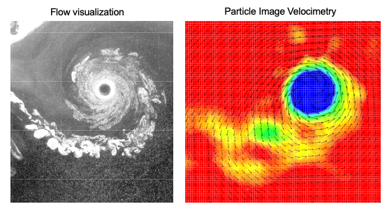
A closer inspection shows that the vortex flow is predominantly laminar near the inner or core region, marked by a very smooth flow region with no interactions between adjacent fluid layers. A more detailed study shows that any turbulence present inside this region will be either relaminarized or suppressed; even substantial eddies will not be able to penetrate this vortex boundary. Moving radially outward from the darker void, it can be seen that this smooth region is followed by a transitional region with regions of both smooth flow and turbulent flow with eddies of different sizes. Further outside this transition zone is a more highly turbulent region. This multi-region vortex structure concept differs from the descriptions assumed by mathematical models in that the flow is neither completely laminar nor thoroughly turbulent.

The second image above is a velocity field measurement of the swirling vortex flow, the velocity vectors shown by the arrows. The measurements were made using the Particle Image Velocimetry (PIV) technique, which uses thin sheets of high-energy laser light to illuminate the flow region of interrogation. The flow must be seeded first with tiny smoke particles, which are injected into the flow. The lasers flash in quick succession (micro-seconds separate the beams), and digital cameras capture images of the movement of the smoke particles, which, on first examination, look like star fields. The images can then be processed numerically to determine the particle movements and the resulting velocity field.

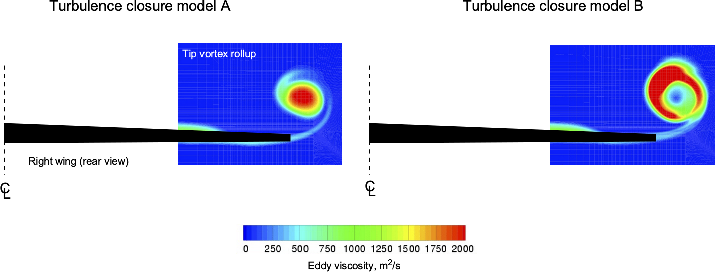
These observations and measurements are critical to the verification and validation (V & V) of computational methods, i.e., computational fluid dynamics or CFD. For example, the figure below shows CFD predictions of the wing tip vortex rollup using two different turbulence models, called turbulent closure models. Even though both solutions give similar bulk flow properties, different detailed quantitative properties and turbulence levels are obtained. As to which results are “correct” can only be reconciled with respect to detailed measurements made in experiments, such as in the wind tunnel. Even then, more measurements may be needed to ensure that the CFD predicts the correct physical behavior for the proper reasons.

Summary & Closure

The ability to classify fluid flows is the first step in understanding flows and developing mathematical models to solve for such fluid flows. Classifications of fluid flows include fully laminar or turbulent flow and/or steady or unsteady flow. The solution of laminar flows is relatively straightforward compared to turbulent flows and can be solved using deterministic mathematical models. However, including the dimension of time in the solution of fluid flows makes analyzing such unsteady flows commensurately more difficult. Turbulent flows are generally the most difficult to understand and predict because they are unsteady and non-deterministic, so statistical methods must be used to describe them. Most practical problems in aerodynamics involve turbulent flows of one kind or another, which contain eddies of various scales. Accurately predicting turbulent flows remains a challenge, but progress continues to be made in this area, and researchers are working to improve the understanding of turbulence and its role in aerodynamics.