Turbulent Flows

J. Gordon Leishman

31 Turbulent Flows

Introduction

Turbulent or mixing flows can occur in all types of fluids. The creation of turbulence results from natural instabilities that quickly form in a smooth laminar flow. The attainment of a certain specific or critical Reynolds number, a parameter named after the pioneering work of Osborne Reynolds, determines the conditions for the natural transition from laminar to turbulent flows. However, other external factors can also influence the onset of turbulence, the amount of turbulence generation, and its eventual dissipation. 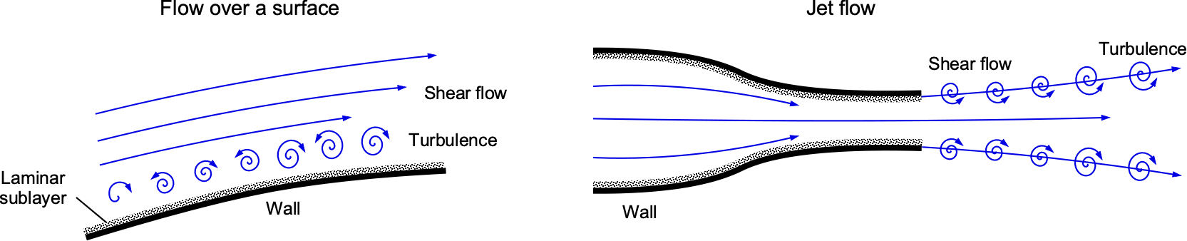Turbulence results from shearing stresses created by velocity gradients in a viscous fluid, e.g., stresses such as $\mu (\partial u/ \partial y)$ , $\mu (\partial v / \partial x)$ , etc. Shear flows and the corresponding shear stresses will be produced near any solid boundary (i.e., walls) because of the no-slip condition on the walls, as shown in the figure below. Shear stresses also occur at interfaces between fluid streams flowing at different velocities, e.g., at the edges of wakes and jets.

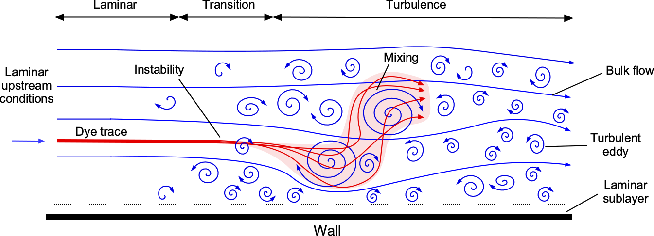
Turbulence will be produced in flows near solid boundaries and other sheared flows.

A random, irregular motion of the fluid elements is a characteristic of turbulent flows. In fluid dynamics, the term “turbulent flows” is usually used instead of “turbulence,” but both terms can be used synonymously in most contexts. The creation of turbulent flows or turbulence is often referred to as a “chaotic” or stochastic process. It involves changes in local flow velocity and pressure fluctuations from the formation of vortices and eddies, as shown in the schematic below. In a laminar flow, the fluid particles follow the streamlines precisely, as indicated by the linear dye trace in the laminar region. Turbulent flow involves the superposition of the effects of eddies of various sizes onto the mean flow. The dye’s path, therefore, is influenced by both the bulk or mean flow (i.e., the time-averaged or mean streamlines) and the location and strength of the eddies. Larger eddies can carry the dye across the mean streamlines, introducing considerable mixing in the flow. Additionally, smaller eddies will contribute to further mixing, causing the dye to diffuse quickly.

Turbulence creates eddies, generating more eddies in a cascading mixing process.

One of the characteristic features of turbulent flows is its multi-scale nature – the bigger eddies generate smaller eddies and then increasingly smaller eddies, a process postulated by Kolmogorov’s hypothesis. Therefore, turbulent flows about airplanes consist of a hierarchy of eddy scales, from the order of the scale of the wing chord down to those of a few millimeters. The smaller-scale eddies, such as those remaining residual in a flow after a disturbance has ended, eventually spin down and dissipate their rotational and translational energy as heat under the action of shear forces caused by viscosity. Richard Feynman described “turbulence” as one of classical physics’s most important unsolved problems.^[1]. However, explaining turbulence is probably the most important unsolved problem in mathematics, not physics.

Engineers attempt to mathematically model turbulent flows, such as within the framework of the Navier-Stokes equations, because the consequences of turbulent flows come into the solution of so many real-world problems. Turbulent flow modeling is needed to optimize aircraft performance, predict the weather, and better understand chemical reactions and energy production. Turbulence comes into play in most aerodynamic problems, as well as combustion, heat transfer, fluid-structure interactions, and noise generation. Turbulent flows cause increased drag on aircraft, mainly from the higher skin friction produced by turbulent boundary layers. Turbulent flows also cause thicker boundary layers, which increases the pressure drag on lifting surfaces. However, turbulent flows are also specifically harnessed in engineering applications, such as fuel mixing in engines and combustion processes and efficient heat transfer in industrial processes. Turbulent flows can also be used in some cases to keep flows attached to lifting surfaces where otherwise they would separate, i.e., the use of vortex generators, a form of flow control.

Learning Objectives

Understand the physical nature of turbulent flows, which are inherently unsteady.
Appreciate why the effects of turbulent flows are challenging to model within the governing equations of fluid behavior.
Know the meaning of Reynolds decomposition and how it is used.
Understand how to develop the Reynolds-Averaged Navier-Stokes (RANS) equations.
Appreciate the concept of eddy viscosity and how it can represent turbulent flows.

Visualizing Turbulent Flows

In the 16th century, the great polymath Leonardo da Vinci made sketches of turbulent flows, two of which are shown below, taken from his famous notebooks (codex). He described the existence of whirlpools and “whorls” or eddies and wrote, “Observe the motion of the surface of the water, resembling that of hair, which has two motions, of which one is caused by the weight of the hair, the other by the direction of the whorls; thus the water has whorling motions, one part of which is from the principal current, the other to random and reverse motion.”^[2] In other words, Leonardo da Vinci explains the essence of a turbulent flow, with whorls and vortices of various sizes formed, causing some level of ordered three-dimensional fluid motion, usually referred to as the bulk flow, and some level of disordered or random motions, which is now referred to as “turbulence.”

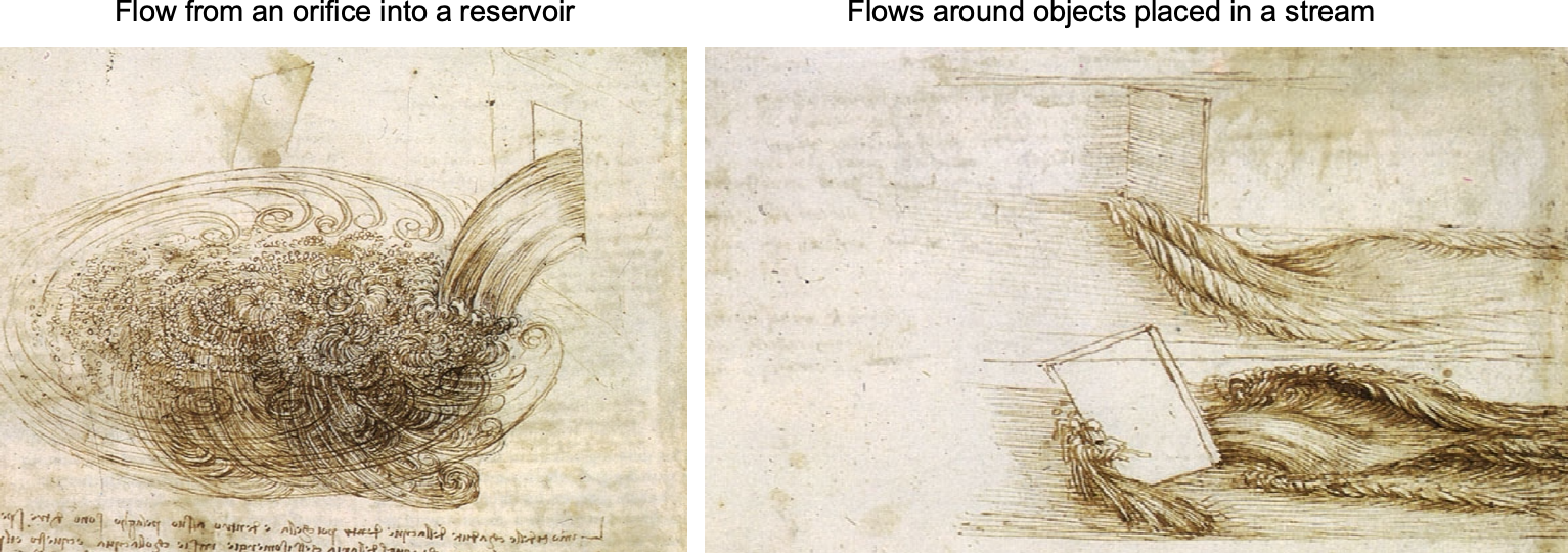
Sketches made by Leonardo da Vinci of turbulent flows. From the “Atlantic Codex.”

Da Vinci also noted, “The small whorls are almost numberless, and large things are rotated only by large whorls and not by small ones, but both turn small whorls.” Da Vinci also states, “So moving water strives to maintain the course under the power which occasions it and, if it finds an obstacle in its path, completes the span of the course it has commenced by a circular and revolving movement.” These profound observations, perhaps the first documented flow visualizations of turbulence, have since formed a basis for scientifically and describing turbulent flows in terms of mathematics.

The visualization image below shows another example that documents the fascinating natural creation of a turbulent flow. The refractive or schlieren effects originate from a heat source (a candle in this case), which initially causes a flow to rise vertically upward as a smooth laminar jet. At some point downstream, depending on the Reynolds number, the flow begins to transition to turbulent flow. This process is characterized by forming relatively large eddies, which causes increasing mixing levels in the flow.

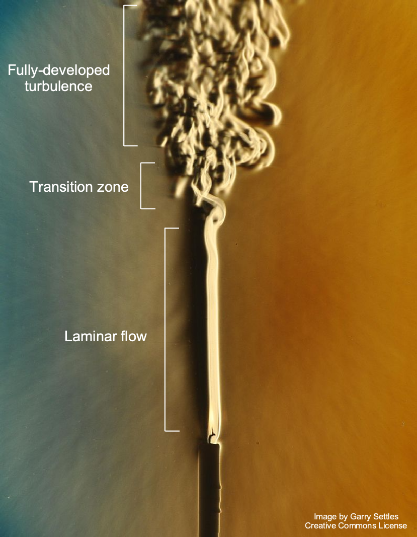
Schlieren flow visualization of the transition of a smooth laminar flow to one with turbulence.

Notice from the image above that the mixing proceeds very quickly as the flow develops, soon becoming more turbulent and the boundaries of the thermal jet rapidly expanding. The expansion occurs because the turbulent mixing slows the average bulk flow, so mass conservation (continuity) means the wake expands. Images such as these confirm that turbulent flows involve energy transfer across various physical scales; the initial larger-scale eddies, on average, break down into medium and then ever-smaller eddies. This energy cascade continues until it reaches the smallest scales, where the energy is eventually dissipated under the action of viscosity. Recall that viscosity is the property of a fluid that resists deformation, so it acts as a dissipative energy mechanism. Therefore, the kinetic energy in the turbulence is ultimately converted into heat through shear and viscous dissipation.

What is the difference between an “eddy” and a “vortex”?

An eddy and a vortex are fluid dynamics phenomena with vorticity and circulation, but they usually refer to different swirling fluid motions. An eddy is a swirling fluid that moves in a circular or spiral manner. Eddies, sometimes called whorls, are typically found in the wake of obstacles or areas where fluid flow is sheared, causing swirling motion. Still, they are relatively small-scale compared to vortex phenomena. A vortex is a more general term for any swirling flow and can encompass larger-scale phenomena such as wing-tip vortices, tornadoes, and hurricanes.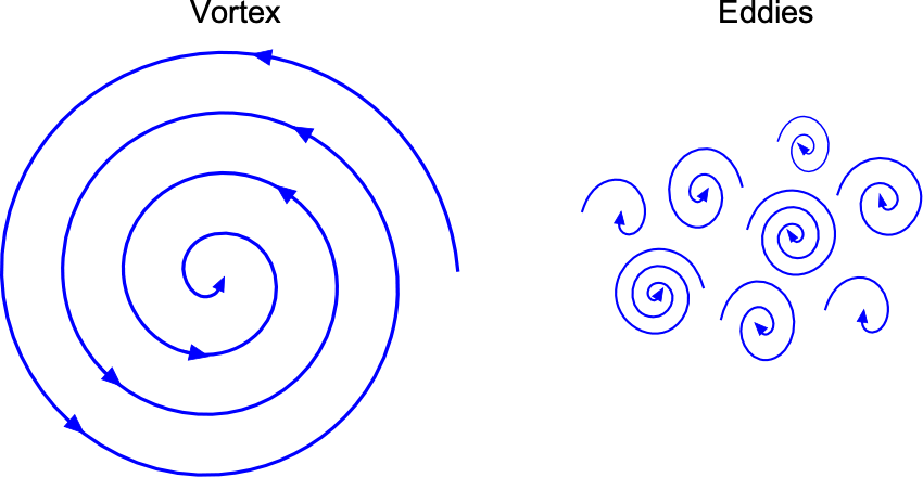

Reynolds Decomposition

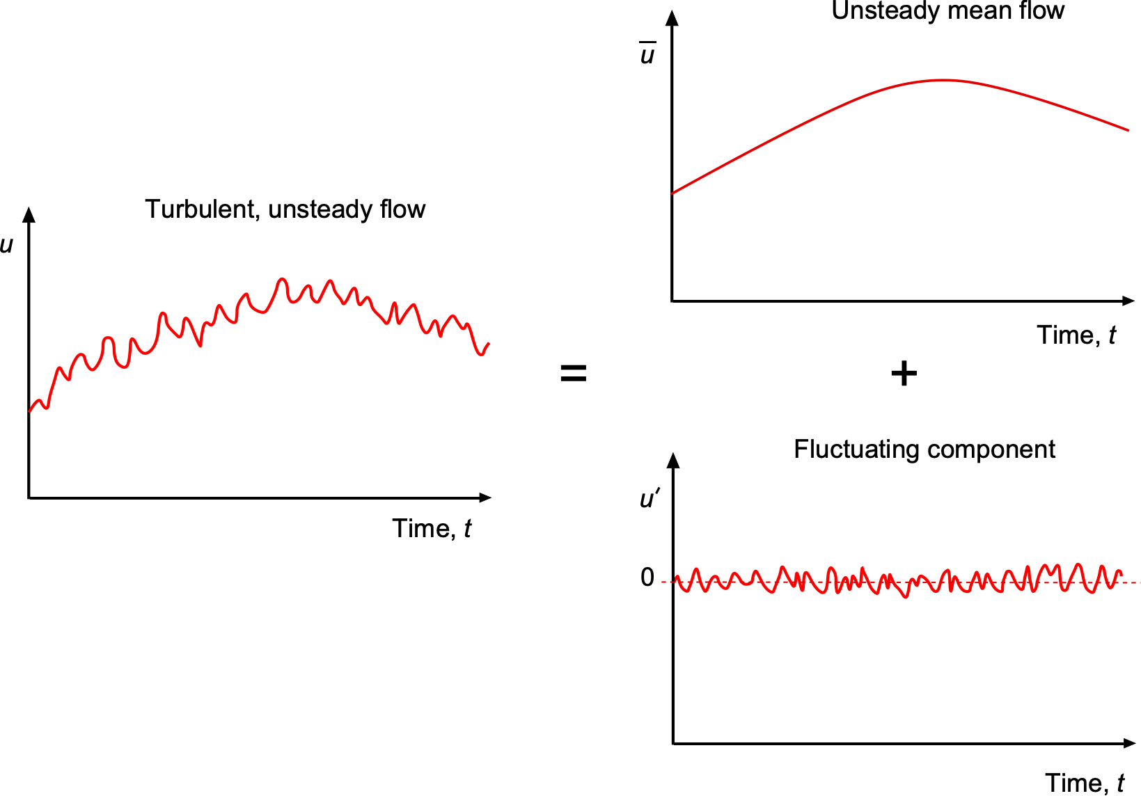
One of the techniques by which engineers model turbulent flows is by using a Reynolds decomposition. In this method, an instantaneous flow property such as a velocity, $u(t)$ , is decomposed into a mean value of velocity, $\overline{u}$ , with an associated fluctuating component, $u'$ , i.e., the flow velocity can be expressed as $u = \overline{u} + u'$ , as shown in the figure below. Each fluctuation of $u'$ is associated with an eddy or group of eddies in the flow, which may cause the local flow velocity to increase or decrease depending on the sign of rotation of the eddy, i.e., clockwise or counterclockwise, and the proximity of the eddy to the measurement point. Reynolds decomposition is a critical concept in the mathematical models used to describe turbulent flows, resulting in a set of very useful governing equations to solve for the flow properties called the Reynolds-Averaged Navier-Stokes (RANS) equations.

Reynolds decomposition can also be extended to three dimensions, where each velocity component or scalar quantity can be separately decomposed into its own mean and fluctuating component. This approach leads to a more complete description of the three-dimensional turbulent flow and enables a better understanding of the fluid transport phenomena that occur in turbulent flows. For example, if Reynolds decomposition is applied to the three components of the flow velocity, then

(1) $\begin{eqnarray*} u(x, y, z, t) & = & \overline{u(x, y, z)} + u' (x, y, z, t) \\[8pt] v(x, y, z, t) & = & \overline{v(x, y, z)} + v' (x, y, z, t) \\[8pt] w(x, y, z, t) & = & \overline{w(x, y, z)} + w' (x, y, z, t) \end{eqnarray*}$

where the $\overline{u}$ , $\overline{v}$ , and $\overline{w}$ terms are the mean values of the flow velocity, and the $u'$ , $v'$ , and $w'$ terms are the associated fluctuating components from the mean, respectively. Notice that the $u$ , $v$ , and $w$ as well as $u'$ , $v'$ , and $w'$ are functions of time and space but the averages $\overline{u}$ , $\overline{v}$ , and $\overline{w}$ are functions of space only.

The mean values can be obtained by averaging the flow properties over a long period, say $T$ , so that for a given spatial location in the flow, say $(x, y, z)$ , then

(2) $\begin{eqnarray*} \overline{u(x, y, z)} & = & \left( \frac{1}{T} \right)\lim_{T \rightarrow \infty} \, \left( \int_t^{t + T} u(x, y, z, t) \ d t \right) \\[8pt] \overline{v(x, y, z)} & = & \left( \frac{1}{T} \right) \lim_{T \rightarrow \infty} \, \left( \int_t^{t + T} v(x, y, z, t) \ d t \right) \\[8pt] \overline{w(x, y, z)} & = & \left( \frac{1}{T} \right) \lim_{T \rightarrow \infty} \, \left( \int_{t}^{t + T} w(x, y, z, t) \ d t \right) \end{eqnarray*}$

How long $T$ needs to be to obtain the desired information depends on the flow. The general rule is that $T$ must be long enough for statistical convergence, which often means as long as practically possible within the times and constraints of any experiment. Formal convergence studies may also need to be performed so that the results are within accepted statistical bounds. Therefore, the turbulent parts of the flow velocities are

(3) $\begin{eqnarray*} {u'(x, y, z, t)} & = & {u(x, y, z, t)} - \overline{u(x, y, z)} \\[8pt] {v'(x, y, z, t)} & = & {v(x, y, z, t)} - \overline{v(x, y, z)} \\[8pt] {w'(x, y, z, t )} & = & {w(x, y, z, t)} - \overline{w(x, y, z)} \end{eqnarray*}$

from which the root mean square (rms) or “strength” of the turbulent flow can be defined as

(4) $\begin{eqnarray*} {u_{\rm rms}(x, y, z)} & = & \sqrt{\, \overline{u'(x, y, z, t)^2}} \\[8pt] {v_{\rm rms}(x, y, z)} & = & \sqrt{\, \overline{v'(x, y, z, t)^2}} \\[8pt] {w_{\rm rms}(x, y, z)} & = & \sqrt{\, \overline{w'(x, y, z, t)^2}} \end{eqnarray*}$

In practice, these averaged values are found from discrete values (i.e., flow measurements made at discrete time intervals), so summations replace the integrals. For a discretely sampled time-history of $N$ values on statically correlated three-component measurements of velocity $(u, v, w)$ , then performing Reynolds decomposition gives the mean velocity components as

(5) $\begin{eqnarray*} \overline{{u}(x, y, z)} & = & \left( \frac{1}{N} \right) \sum_{n=1}^N {u}_n(x, y, z, t) \\[8pt] \overline{{v}(x, y, z)} & = & \left( \frac{1}{N} \right) \sum_{n=1}^N {v}_n (x, y, z, t) \\[8pt] \overline{{w}(x, y, z)} & = & \left( \frac{1}{N} \right) \sum_{n=1}^N {w}_n (x, y, z, t) \end{eqnarray*}$

where $N$ is the number of contiguous measurements to ensure statistical validity. The value of $N$ must be sufficiently large that statistical convergence is obtained, typically needing thousands of samples. Some turbulent events may occur sporadically and/or have brief durations, so contiguous measurements are essential to capture their behavior fully. For unsteady flows, especially periodic flows, phase-averaging may be needed; in this process, the mean flow values are obtained by summing the measured values over many cycles in phase based on some periodic trigger or other defined event.

Reynolds’ Rules of Averaging

The rules of statistical averaging are important when setting up the form of the RANS equations that will allow their solution. If $a$ and $b$ are fluctuating quantities varying in time such that

(6) $\begin{equation*} a = \overline{a} + a' \quad \mbox{\small and} \quad b = \overline{b} + b' \end{equation*}$

then certain rules called the Reynolds averaging rules, which are given below, will apply. These rules follow statistical precedents from mathematics, and it is a straightforward exercise to prove that they follow from Eq. 6.

The average of the sum is the sum of the averages, i.e.,

(7) $\begin{equation*} \overline{a + b} = \overline{a} + \overline{b} \end{equation*}$

The average of the turbulent values is zero, so

(8) $\begin{equation*} \overline{a'} = \overline{b'} = 0 \quad \mbox{\small and } \quad \overline{a'} + \overline{b'} = 0 \end{equation*}$

Constants do not affect and are not affected by averaging, i.e.,

(9) $\begin{equation*} \overline{k \, a} = k \, \overline{a} \quad \mbox{\small where $k$ is a constant.} \end{equation*}$

The average of the product is the sum of the averages

(10) $\begin{equation*} \overline{a \, b} = \overline a \, \overline b + \overline{a' \, b'} \end{equation*}$

Averaging products also leads to

(11) $\begin{equation*} \overline{a \, a} = \overline a \, \overline a + \overline{a' \, a'} \quad \mbox{\small so that} \quad \overline{a^2} = \overline a^2 + \overline{a'}^2 \end{equation*}$

In terms of the derivatives found in the Navier-Stokes equations, then the average of the time or space derivative of a quantity is equal to the corresponding derivative of the average, i.e.,

(12) $\begin{equation*} \dfrac{\overline{\partial a}}{\partial t} = \dfrac{\partial \overline{a}}{\partial t} \quad \mbox{ \small and } \quad \dfrac{\overline{\partial a}}{\partial x} = \dfrac{\partial \overline{a}}{\partial x} \end{equation*}$

Navier-Stokes Equations

Recall that the incompressible form of the Navier-Stokes equations can be written as

(13) $\begin{equation*} \varrho \frac{D \vec{V}}{Dt} = -\nabla p + \mu \nabla^2 \,\vec{V} \end{equation*}$

where $\nabla^2$ is the vector Laplacian. Notice that

(14) $\begin{equation*} \nabla^2 \,\vec{V} = \nabla \bigcdot \nabla \vec{V} \end{equation*}$

so the viscous terms are shear terms that depend on the velocity gradients in the flow, i.e., $\partial u/\partial y$ , $\partial w/\partial x$ , etc. These terms can be referred to as the Newtonian shear stresses. The Navier-Stokes equations can also be written in the form

(15) $\begin{equation*} \frac{D \vec{V}}{Dt} = -\frac{1}{\varrho} \nabla p + \left( \frac{\mu}{\varrho} \right) \nabla^2 \,\vec{V} = -\frac{1}{\varrho} \nabla p + \nu \nabla^2 \,\vec{V} \end{equation*}$

where $\nu$ is the kinematic viscosity; this latter form is the most common way of writing the Navier-Stokes equations.

Notice that there is nothing in the assumptions and derivation of the Navier-Stokes equations to suggest that they are limited to laminar flows. However, as they stand in their most basic form, they are not helpful for application to turbulent flows because the appropriate initial and boundary conditions cannot be defined. However, this dilemma can be resolved with the use of Reynolds averaging. Proceeding by expanding out the substantial derivative in Eq. 13 gives

(16) $\begin{equation*} \varrho \left(\frac{\partial \vec{V}}{\partial t} + \vec{V} \bigcdot \nabla \, \vec{V}\right) = -\nabla p + \mu \nabla^2 \,\vec{V} \end{equation*}$

and in terms of their scalar components, then

(17) $\begin{eqnarray*} \varrho \left(\frac{\partial u}{\partial t} + u \bigcdot \nabla u \right) & = & -\frac{\partial p}{\partial x} + \mu \left(\frac{\partial^2 u}{\partial x^2} + \frac{\partial^2 u}{\partial y^2} + \frac{\partial^2 u}{\partial z^2}\right) \\[8pt] \varrho \left(\frac{\partial v}{\partial t} + v \bigcdot \nabla v \right) = & = & -\frac{\partial p}{\partial y} + \mu \left(\frac{\partial^2 v}{\partial x^2} + \frac{\partial^2 v}{\partial y^2} + \frac{\partial^2 v}{\partial z^2}\right) \\[8pt] \varrho \left(\frac{\partial w}{\partial t} + w \bigcdot \nabla w \right) & = & -\frac{\partial p}{\partial z} + \mu \left(\frac{\partial^2 w}{\partial x^2} + \frac{\partial^2 w}{\partial y^2} + \frac{\partial^2 w}{\partial z^2}\right) \end{eqnarray*}$

which become

(18) $\begin{eqnarray*} \varrho \left(\frac{\partial u}{\partial t} + u \frac{\partial u}{\partial x} + v \frac{\partial u}{\partial y} + w \frac{\partial u}{\partial z}\right) & = & -\frac{\partial p}{\partial x} + \mu \left(\frac{\partial^2 u}{\partial x^2} + \frac{\partial^2 u}{\partial y^2} + \frac{\partial^2 u}{\partial z^2}\right) \\[8pt] \varrho \left(\frac{\partial v}{\partial t} + u \frac{\partial v}{\partial x} + v \frac{\partial v}{\partial y}+ w \frac{\partial v}{\partial z}\right) & = & -\frac{\partial p}{\partial y} + \mu \left(\frac{\partial^2 v}{\partial x^2} + \frac{\partial^2 v}{\partial y^2} + \frac{\partial^2 v}{\partial z^2}\right) \\[8pt] \varrho \left(\frac{\partial w}{\partial t} + u \frac{\partial w}{\partial x} + v \frac{\partial w}{\partial y}+ w \frac{\partial w}{\partial z}\right) & = & -\frac{\partial p}{\partial z} + \mu \left(\frac{\partial^2 w}{\partial x^2} + \frac{\partial^2 w}{\partial y^2} + \frac{\partial^2 w}{\partial z^2}\right) \end{eqnarray*}$

For steady flows, then the equations are reduced to

(19) $\begin{equation*} \varrho \left( \vec{V} \bigcdot \nabla \, \vec{V}\right) = -\nabla p + \mu \nabla^2 \,\vec{V} \end{equation*}$

and in terms of the scalar components, they are

(20) $\begin{eqnarray*} \varrho \left(u \frac{\partial u}{\partial x} + v \frac{\partial u}{\partial y} + w \frac{\partial u}{\partial z}\right) & = & -\frac{\partial p}{\partial x} + \mu \left(\frac{\partial^2 u}{\partial x^2} + \frac{\partial^2 u}{\partial y^2} + \frac{\partial^2 u}{\partial z^2}\right) \\[8pt] \varrho \left(u \frac{\partial v}{\partial x} + v \frac{\partial v}{\partial y}+ w \frac{\partial v}{\partial z}\right) & = & -\frac{\partial p}{\partial y} + \mu \left(\frac{\partial^2 v}{\partial x^2} + \frac{\partial^2 v}{\partial y^2} + \frac{\partial^2 v}{\partial z^2}\right) \\[8pt] \varrho \left( u \frac{\partial w}{\partial x} + v \frac{\partial w}{\partial y}+ w \frac{\partial w}{\partial z}\right) & = & -\frac{\partial p}{\partial z} + \mu \left(\frac{\partial^2 w}{\partial x^2} + \frac{\partial^2 w}{\partial y^2} + \frac{\partial^2 w}{\partial z^2}\right) \end{eqnarray*}$

Including Turbulent Flow Effects

Reynold decomposition and the averaging rules can now be applied to the continuity and momentum equations. The outcome will be the Reynolds-Averaged Navier-Stokes equations or RANS equations. This form of the Navier-Stokes equations forms the basis of most CFD simulations of complex flows.

Continuity

For a steady, incompressible flow, the continuity equation is

(21) $\begin{equation*} \nabla \bigcdot \vec{V} = \frac{\partial u}{\partial x} + \frac{\partial v}{\partial y} + \frac{\partial w}{\partial z} = 0 \end{equation*}$

so, in terms of the Reynolds decomposition, then

(22) $\begin{equation*} \frac{\partial (\overline{u} + u')}{\partial x} + \frac{\partial (\overline{v} + v')}{\partial y} + \frac{\partial (\overline{w} + w')}{\partial z} = 0 \end{equation*}$

Taking only the mean value of Eq. 23 gives

(23) $\begin{equation*} \frac{\partial \overline{u}}{\partial x} + \frac{\partial \overline{v} }{\partial y} + \frac{\partial \overline{w} }{\partial z} = 0 \end{equation*}$

and subtracting Eq. 23 from Eq. 21 gives

(24) $\begin{equation*} \frac{\partial u'}{\partial x} + \frac{\partial v'}{\partial y} + \frac{\partial w'}{\partial z} = 0 \end{equation*}$

Therefore, the mean or bulk flow $(\overline{u}, \overline{v}, \overline{w} )$ in terms of Eq. 23 and the fluctuating flow $(u', v', w' )$ in terms of Eq. 24 both satisfy continuity.

Momentum

The momentum terms can now be considered. By first multiplying Eq. 21 by $u$ and adding it to the left-hand-side of the $x$ component of the momentum equation in Eq. 20, then

(25) $\begin{equation*} {\rm LHS} = \varrho \left(u \frac{\partial u}{\partial x} + v \frac{\partial u}{\partial y} + w \frac{\partial w}{\partial z} \right) + \varrho \, u \left( \dfrac{\partial u}{\partial x} + \dfrac{\partial v}{\partial y} + \dfrac{w}{\partial z} \right) \end{equation*}$

Therefore, the mathematics leads to

(26) $\begin{equation*} 0 = \frac{\partial}{\partial x} \left( -p + \mu \frac{\partial u}{\partial x} - \varrho u^2 \right) + \frac{\partial}{\partial y} \left( \mu \frac{ \partial u}{\partial y } - \varrho u v \right) + \frac{\partial}{\partial z} \left( \mu \frac{\partial u}{\partial z} - \varrho u w \right) \end{equation*}$

The pressure is $\overline{p} + p'$ , and the three velocities are $\overline{u} + u'$ , $\overline{v} + v'$ , $\overline{w} + w'$ , respectively. Therefore, assuming a steady flow and taking only the mean values gives

(27) $\begin{equation*} 0 = -\frac{\partial \overline{p}}{\partial x} + \mu \nabla^2 \left( \overline{\overline{u} + u '} \right) - \varrho \left( \frac{\partial (\overline{u}^2)}{\partial y} + \frac{\partial (\overline{u v})}{\partial z} + \frac{\partial (\overline{u w})}{\partial z} \right) \end{equation*}$

and so

(28) $\begin{equation*} 0 = -\frac{\partial \overline{p}}{\partial x} + \mu \nabla^2 \,\overline{u} - \varrho \left( \frac{\partial (\overline{u}^2)}{\partial x} + \frac{\partial (\overline{u} \overline{v})}{\partial y} + \frac{\partial (\overline{u w})}{\partial z} \right) - \varrho \left( \frac{\partial (\overline{u' u' })}{\partial x} + \frac{\partial (\overline{u' v'})}{\partial y} + \frac{\partial (\overline{u' w'})}{\partial z} \right) \end{equation*}$

Then subtracting $\varrho \, \overline{u}$ times Eq. 23 from the first term in parentheses on the left-hand-side in Eq. 28 gives

(29) $\begin{equation*} 0 = -\frac{\partial \overline{p}}{\partial x} + \mu \nabla^2 \,\overline{u} - \varrho \left( \overline{u} \frac{\partial \overline{u}}{\partial x} + \overline{v} \frac{\partial \overline{u}}{\partial y} + \overline{w}\frac{\partial \overline{u}}{\partial z} \right) - \varrho \left( \frac{\partial (\overline{u' u'})}{\partial x} + \frac{\partial (\overline{u' v'})}{\partial y} + \frac{\partial (\overline{u' w'}) }{\partial z} \right) \end{equation*}$

or

(30) $\begin{equation*} \varrho \left( \overline{u} \frac{\partial \overline{u}}{\partial x} + \overline{v} \frac{\partial \overline{u}}{\partial y} + \overline{w} \frac{\partial \overline{u}}{\partial z} \right) = -\frac{\partial \overline{p}}{\partial x} + \mu \nabla^2 \,\overline{u} -\varrho \left( \frac{\partial (\overline{u' u' })}{\partial x} + \frac{\partial (\overline{u' v'})}{\partial y} + \frac{\partial ( \overline{u' w'}) }{\partial z} \right) \end{equation*}$

The corresponding equations for the $y$ and $z$ directions are

(31) $\begin{equation*} \varrho \left( \overline{u} \frac{\partial \overline{v}}{\partial x} + \overline{v} \frac{\partial \overline{v}}{\partial y} + \overline{w} \frac{\partial \overline{v}}{\partial z} \right) = -\frac{\partial \overline{p}}{\partial y} + \mu \nabla^2 \,\overline{v} - \varrho \left( \frac{\partial (\overline{v' u' })}{\partial x} + \frac{\partial (\overline{v' v'})}{\partial y} + \frac{\partial (\overline{v' w'})}{\partial z} \right) \end{equation*}$

and

(32) $\begin{equation*} \varrho \left( \overline{u} \frac{\partial \overline{w}}{\partial x} + \overline{v} \frac{\partial \overline{w}}{\partial y} + \overline{w} \frac{\partial \overline{w}}{\partial z} \right) = -\frac{\partial \overline{p}}{\partial z} + \mu \nabla^2 \,\overline{v} - \varrho \left( \frac{\partial (\overline{w' u' })}{\partial x} + \frac{\partial (\overline{w' v'})}{\partial y} + \frac{\partial (\overline{w' w'})}{\partial z} \right) \end{equation*}$

which can finally be written in the elegant vector form of the Navier-Stokes equation as

(33) $\begin{equation*} \varrho \left( \vec{\overline{V}} \bigcdot \nabla \, \vec{\overline{V}}\right) = -\nabla \overline{p} + \mu \nabla^2 \,\vec{\overline{V}} -\nabla \bigcdot \tau^R \end{equation*}$

which are called the Reynolds-Averaged Navier Stokes (RANS) equations. Recalling the original form of the Navier-Stokes equations, i.e., their “laminar” form without the turbulent flow terms, then

(34) $\begin{equation*} \varrho \left( \vec{V} \bigcdot \nabla \, \vec{V}\right) = -\nabla p + \mu \nabla^2 \,\vec{V} \end{equation*}$

so it can be seen that Eq. 33 differs from the original form of the Navier-Stokes equation in Eq. 34 because of the addition of the $\nabla \bigcdot \tau^R$ term on the right-hand side, which is called the Reynolds stress tensor. The stress tensor, which is a matrix of stress terms, accounts for the additional effects of turbulent flow on the momentum transfer and can be expressed as

(35) $\begin{equation*} \tau^R = \begin{bmatrix} \tau_{xx} & \tau_{xy} & \tau_{xz} \\[12pt] \tau_{yx} & \tau_{yy} & \tau_{yz} \\[12pt] \tau_{zx} & \tau_{zy} & \tau_{zz} \end{bmatrix} = \varrho \begin{bmatrix} \overline{ u' u'} & \overline{ u' v'} & \overline{ u' w'} \\[12pt] \overline{ v' u'} & \overline{ v' v'} & \overline{ v' w'} \\[12pt] \overline{ w' u'} & \overline{ w' v'} & \overline{ w' w'} \end{bmatrix} \end{equation*}$

Therefore, the terms $\varrho \, \overline{ u' u'} = \tau_{xx}$ , $\varrho \, \overline{ u' v'} = \tau_{yx}$ , $\varrho \, \overline{ u' w'} = \tau_{zx}$ , etc., play a role of contributing additional stresses in the flow over and above that caused by viscosity alone. However, out of the nine total Reynolds stresses, only six are distinct or unique because the stress tensor is symmetric, i.e., $\overline{ u' v'} = \overline{ v' u'}$ , $\overline{ u' w'} = \overline{ w' u'}$ , and $\overline{ v' w'} = \overline{ w' v'}$ . Notice that the diagonal terms in the matrix represent the normal compressive stresses in the fluid, and the off-diagonal terms are the shear stresses.

The preceding equations describe the motion of a turbulent flow, albeit approximately within the statistical approximations that have been assumed. However, the appearance of the six Reynolds stresses means that the number of unknowns has, in effect, increased to ten (pressure, three components of the flow velocity, and six Reynolds stress terms), while only four equations are available, so the properties cannot be uniquely solved. Further progress requires additional equations to relate the Reynolds stresses to the flow velocity components. Indeed, the fundamental problem of turbulence modeling within the framework of the RANS equations is to find six additional mathematical relations to close out the system of these four equations.

What are the units of the Reynolds stress terms?

The units of terms such as $\varrho \, \overline{ u' u'}$ will be

$\left[ \varrho \, \overline{ u' u'} \right] = \rm \left( M L^{-3} \right) \left(L T^{-1} \right) \left(L T^{-1} \right) = M L^{-1} T^{-2} = \frac{M L T^{-2}}{L^2} \equiv \frac{\mbox{\small Force}}{\mbox{\small Area}}$

A force per unit area is a stress, so these terms are indeed stresses.

Eddy Viscosity Models

Notice that the viscous stresses can all be written in the form

(36) $\begin{equation*} {\nu}\frac{\partial^2 \overline{u}}{\partial y^2}-\frac{\partial}{\partial y}(\overline{u' v'}) = \frac{\partial}{\partial y} \left( \nu\frac{\partial \overline{u}}{\partial y}- (\overline{u' v'}) \right) = \frac{\partial \left( \tau_l + \tau_t \right)}{\partial y} \end{equation*}$

Therefore, the sum of a laminar shear stress component and a turbulent shear stress component, in effect, replaces the “laminar” viscous stresses. This means that

(37) $\begin{equation*} \tau_t = - \overline{u' v'} = \mu_t \left( \frac{\partial \overline{u}}{\partial y} \right) \end{equation*}$

where $\mu_t$ is called the eddy viscosity, i.e., the extra effective level of viscosity caused by turbulence. Therefore, the turbulence models that attempt to represent the variations of eddy viscosity in the flow are called eddy viscosity models. In an eddy viscosity model, higher levels of turbulent stresses are produced by augmenting the otherwise effects of pure molecular viscosity with a turbulent or “eddy'” viscosity coefficient, i.e., the total effective stresses can be represented as

(38) $\begin{equation*} \tau_e = \left( \mu + \mu_t \right) \nabla \vec{\overline{V}} \end{equation*}$

where it is assumed that the turbulent stress tensor is proportional to the mean strain rate tensor multiplied by a constant.

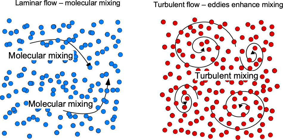
This latter assumption is called the Boussinesq Hypothesis, after Joseph Boussinesq, although never referred to as a hypothesis by Boussinesq himself. However, the assumption or “hypothesis” is reasonable because it assumes that the exchange of turbulent energy in the cascading process of eddies is analogous to the effects of molecular viscosity, as illustrated in the figure below. Experiments and other observations of turbulent flows support such behavior. Therefore, the Boussinesq hypothesis means that the turbulent flow can be modeled as an effective total viscosity that varies with the local flow conditions.

The concept of “eddy” viscosity augments the laminar molecular viscosity from the effects of eddies and mixing caused by turbulence.

The Boussinesq hypothesis is a widely used assumption in fluid mechanics that relates the eddy viscosity, a measure of the turbulent transport of momentum, to the rate of strain tensor in the Navier-Stokes equations. Therefore, with the addition of turbulence in the form of eddy viscosity, the Navier-Stokes equations are now modified into the form

(39) $\begin{equation*} \varrho \left( \vec{\overline{V}} \bigcdot \nabla \, \vec{\overline{V}}\right) = -\nabla \overline{p} + \left( \mu + \mu_t \right) \nabla^2 \,\vec{\overline{V}} \end{equation*}$

Experience has shown that the preceding approach for modeling turbulence within the framework of the Navier-Stokes equations works quite well for certain classes of flow problems, particularly those involving homogeneous mixing and dimensional symmetry and those with relatively isotropic turbulence levels.

Turbulence Scales & Turbulent Kinetic Energy

Eddy viscosity models are in a class of so-called “turbulence models” or “turbulence closure models,” which provide a mathematical basis for solving the mean flow field as well as the turbulent flow quantities. Many different turbulent flow models are available, especially for use within the framework of CFD, and the choice of the “best” or most suitable turbulence model requires careful consideration regarding the problem. The best way to represent the turbulent viscosity and make the decision on the most suitable turbulence model depends on several factors, including the specific flow application, the desired level of accuracy, and the available computational resources.

Deciding on the types of turbulence models that can be expected to give good predictive capability depends on understanding the length and time scales of the specific flow problem in hand. It should be appreciated that turbulent flows exhibit a wide range of spatial scales, each of which plays a vital role in the overall behavior of the flow. The spatial scales of turbulence can be broadly classified into three categories: large, intermediate, and small eddies, as illustrated in the figure below. Therefore, there is no “one size fits all” turbulence model. The different scales of turbulence interact with each other in a complex manner, and a wide range of phenomena, such as vorticity, turbulence intensity, and Reynolds stress, all characterize their behavior. Modeling these scales is crucial for predicting the behavior of turbulent flows, which is a critical challenge in turbulence modeling.

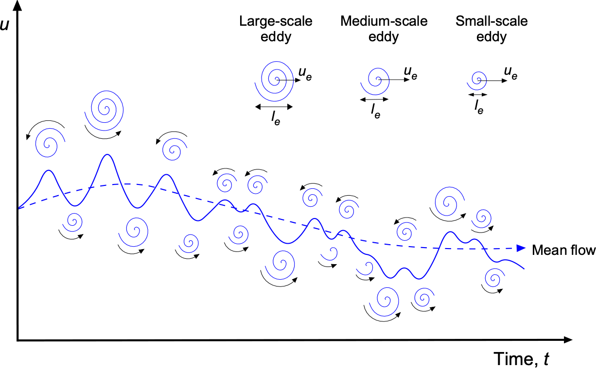
Eddies of different scales and velocities will affect the local flow properties and cause positive and negative fluctuations.

Large-scale eddies are the most significant structures in a turbulent flow. They transport bulk momentum and energy and can cause substantial fluctuations in the local flow properties.
Intermediate-scale eddies: These eddies are smaller than the large-scale eddies but larger than the smallest scales. They are essential in transferring energy from the large-scale eddies to the smallest scales through the “energy cascade” process.
Small-scale eddies: These are the smallest structures, and their linear scales are typically of the order of millimeters or less. They are responsible for energy dissipation and convert the kinetic energy in the flow into thermal energy through viscous shear effects.

Eddy Turnover Time

In turbulent flows, different velocity scales are relevant for understanding the behavior of the flow. These velocity scales are related to the flow’s different lengths and time scales and reflect the different physical phenomena that may occur. They can also be used to classify the overall behavior of the flow. One important time scale in turbulent flows is the eddy turnover time. This time scale is related to the size of the eddies in the flow and reflects how quickly the eddies are breaking down and reforming. The eddy turnover time, $t_e$ , is given by

(40) $\begin{equation*} T_e = \frac{L_e}{U} \end{equation*}$

where $L_e$ is the characteristic length scale of the eddy, and $U$ is the characteristic velocity scale of the eddy. It measures the average time for energy-containing eddies to complete their rotational motion. This time scale is important in the context of the larger turbulent cascade, where energy is transferred from larger to smaller eddy scales.

Eddy Turnover Velocity

The term eddy turnover velocity refers to the characteristic velocity associated with the rotation of eddies in a turbulent flow. In a turbulent fluid motion, eddies are swirling, rotating fluid structures. The eddy turnover velocity measures how quickly these eddies rotate or change their orientation. The eddy turnover velocity is often related to the size and timescale of the eddies by using

(41) $\begin{equation*} U_e = \frac{L_e}{T_e } \end{equation*}$

The turnover velocity provides insight into the nature of the turbulence and the speed at which energy is transferred between different scales of turbulent motion.

Turbulence Intensity

Turbulent intensity measures the turbulence level in a fluid flow, typically expressed as a percentage of the mean flow property. It is defined as the root-mean-square (rms) of the fluctuating property divided by the mean value. In the case of the $u$ component of flow velocity, then

(42) $\begin{equation*} I = \frac{u'_{\rm rms}}{U} \times 100 \quad \mbox{(\small in units of \% of $U$)} \end{equation*}$

where $u'_{\rm rms}$ is the rms of the fluctuating flow component, and $U$ is the mean flow velocity. The mean flow velocity will often be the free-stream reference flow, i.e., $U = U_{\infty}$ or $U = V_{\infty}$ .

The turbulent intensity, $I$ , provides one measure of turbulence “strength” in a fluid flow. Higher intensity values generally indicate more turbulent flows with more significant velocity fluctuations. Measuring turbulent intensity uses techniques such as hot-wire anemometry (HWA) and particle image velocimetry (PIV), which can accurately measure these fluctuations with good temporal resolution. Low turbulence intensities (<1%) are found in the external flow around aircraft. Most wind tunnels have low turbulence levels of less than 1%. Medium turbulence intensities ( about 5%) are found in propellers, fans, and fully developed internal flows. High-speed flows, such as inside turbines and jets, will have greater than 10% turbulence relative to the mean flow.

Turbulent Kinetic Energy

The turbulent kinetic energy, $k$ , also known as the TKE, is an important parameter in fluid dynamics and is often used to characterize the intensity of turbulence in a flow. It is defined by the equation

(43) $\begin{equation*} {\rm TKE} = k = \frac{1}{2} \left( \overline{u'^2} + \overline{v'^2} + \overline{w'^2} \right) \end{equation*}$

TKE is generated when a fluid encounters surfaces, obstacles, or otherwise changes in velocity, with the conversion of mean flow energy into turbulent energy facilitated by turbulent eddies.

The numerical values of the TKE are often used as a validation metric for comparing CFD simulations against flow measurements made in wind tunnels or against other types of CFD models. While not the only validation metric, the TKE provides an excellent basis for assessing the performance of turbulence models. However, uncertainty quantifications of measurements and calculations are needed to ensure valid comparisons and meaningful decisions.

Turbulence Spectra

The kinetic energy contained in turbulence, denoted by $E$ , ranges across a wide range of energy and length scales. This information is usually plotted as a log-log plot of $E(\kappa)$ versus $\kappa$ , as shown in the figure below, for which $\kappa$ is the so-called wave number, as given by

(44) $\begin{equation*} \kappa = \frac{2 \pi}{\mbox{\small Eddy diameter}} = \frac{2 \pi}{l_e} \end{equation*}$

Notice, therefore, that bigger eddies have lower wave numbers, and the smaller eddies have larger wave numbers. The basic idea of this form of presentation is to show the contribution of the turbulent kinetic energy at a particular wave number, $\kappa$ , which results from eddies with characteristic diameter, $l_e$ , and corresponding wavelength $2 \pi/\kappa$ . The use of the wave number originates from the mathematical development of the Kolmogorov universal equilibrium theory, which is one way of characterizing the distribution of turbulence over different lengths and time scales.

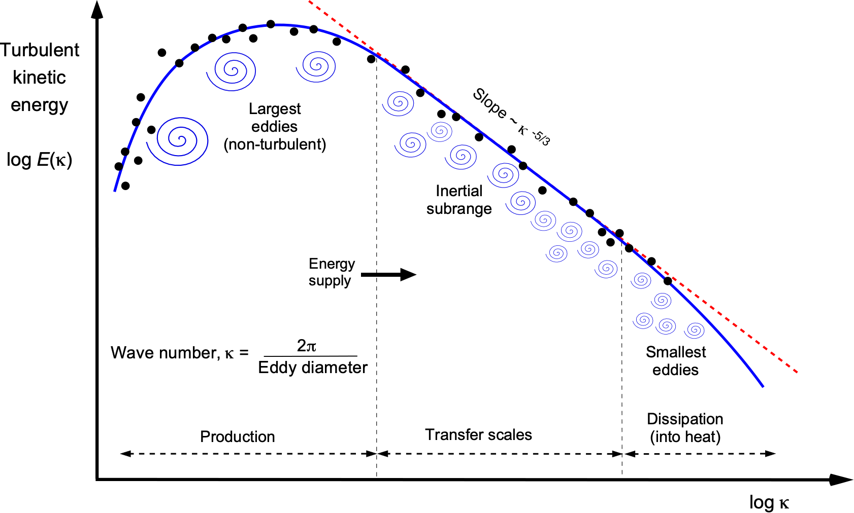
The kinetic energy spectra of turbulence range across many energy and length scales.

The lower left limit of the energy plot corresponds to the length scales at which turbulence is initially generated, i.e., from the biggest eddies. As new eddies are formed and gain energy from the bulk flow, they begin to generate smaller eddies, which then create even smaller eddies in a so-called cascading process. The spectrum of spatial or temporal eddy sizes then reaches a “fully developed” state in which energy is continuously fed from the mean flow into more eddies. This so-called inertial region contains a large portion of the total energy in the turbulence spectrum, which experiments have shown is independent of viscosity, i.e., Reynolds number variations.

The slope in this inertial region is $\kappa^{-5/3}$ , as described by the Kolmogorov theory, as shown by the dashed line in the figure above. This latter behavior, which is characteristic of turbulent flows and occurs in many practical contexts, can also help prescribe the power spectra for turbulence modeling within the framework of a CFD solution, for example. The energy cascading process eventually ends because the smaller eddies continue to break down and become small enough that viscosity causes them to spin down; their remaining kinetic energy then becomes converted to heat.

Wall-Bounded Turbulent Flows

Turbulent boundary layers encapsulate more mixing between the fluid layers and bring higher momentum fluid nearer the wall. Therefore, steeper velocity gradients exist near the wall, with higher shear stresses on the fluid. This is the reason why surfaces like airfoils and wings experience higher drag with turbulent boundary layer flows than with laminar boundary flows. Unfortunately, laminar boundary layers are easily disturbed and quickly develop into turbulent boundary layers, especially at the higher Reynolds numbers typical of actual flight vehicles. In fact, for most airplanes, except perhaps for high-performance sailplanes, laminar boundary layers exist only over very small parts of the leading edges of their wings before they quickly transition into turbulent boundary layers.

Turbulent Boundary Layer Equations

Applying the process of Reynolds decomposition of a turbulent flow gives an alternative subset form of the boundary layer equations, i.e.,

(45) $\begin{eqnarray*} \frac{\partial \overline{u}}{\partial x}+\frac{\partial \overline{v}}{\partial y} & = & 0 \\ \overline{u}\frac{\partial \overline{u}}{\partial x}+\overline{v}\frac{\partial \overline{u}}{ \partial y} & = & -\frac{1}{\varrho} \frac{\partial \overline{p}}{\partial x}+ \nu \left(\frac{\partial^2 \overline{u}}{\partial x^2}+\frac{\partial^2 \overline{u}}{\partial y^2}\right)-\frac{\partial}{\partial y}(\overline{u' v'})-\frac{\partial}{\partial x}(\overline{u'^2}) \\[8pt] \overline{u}\frac{\partial \overline{v}}{\partial x}+\overline{v}\frac{\partial \overline{v}}{ \partial y} & = & -\frac{1}{\varrho} \frac{\partial \overline{p}}{\partial y}+\nu \left(\frac{\partial^2 \overline{v}}{\partial x^2}+\frac{\partial^2 \overline{v}}{\partial y^2}\right)-\frac{\partial}{\partial x}(\overline{u' v'})-\frac{\partial}{\partial y}(\overline{v'^2}) \end{eqnarray*}$

which, like the RANS equations, has created Reynolds stress quantities in terms of the fluctuating velocity components. Notice the pressure is also replaced by a mean value, i.e., $p = \overline{p}$ .

Using the same approach as before with the laminar form of the equation, where the orders of magnitude of the relevant terms in the boundary layer region at the wall were obtained, the form of turbulent boundary layer equations become

(46) $\begin{eqnarray*} \frac{\partial \overline{u}}{\partial x}+\frac{\partial \overline{v}}{\partial y} & = & 0 \\[8pt] \frac{\partial \overline{p} }{ \partial y} & = & 0 \\[8pt] \overline{u}\frac{\partial \overline{u}}{ \partial x}+\overline{v}\frac{\partial \overline{u} }{\partial y} & = & -\frac{1}{\varrho} \frac{\partial \overline{p}}{ \partial x}+{\nu}\frac{\partial^2 \overline{u}}{\partial y^2}-\frac{\partial}{\partial y}(\overline{u' v'}) \end{eqnarray*}$

Again, it can be seen from a comparison with the “laminar” form of the boundary layer equations that the time-averaged values $\overline{u}$ , $\overline{v}$ , and $\overline{p}$ have replaced $u$ , $v$ , and $p$ , respectively. Still, there are also the Reynolds shear stresses to consider in the boundary layer. Reynolds stresses behave in specific ways in boundary layers, and suitable turbulence models must be developed to predict their effects on wings and bodies. The ability to predict, and for the correct reason, is fundamental to the design process.

Mixing Length Theory

It should be appreciated that all of the components of turbulent stresses must approach zero (and hence, so does the eddy viscosity) at solid boundaries (i.e., walls). So, the only stresses that act near the wall are the viscous stresses caused by laminar flows. However, this statement does not imply that the shear stress on the wall is the same as that in a fully laminar boundary layer because they are not. The boundary conditions that must be satisfied are then expressed in terms of the mean velocity components, similar to what is done for a laminar flow. The thin sublayer of the boundary layer next to the wall behaves as a laminar flow, known as a laminar sublayer, where no turbulence exists. In boundary layer problems, the Prandtl mixing-length approach can be used. The assumption is that the turbulence varies in intensity as a function of distance from the wall, $y$ , i.e., turbulence is lower near and higher away from the wall. As shown in the figure below, the definition of mixing length implies that fluid elements migrating from level $a$ to level $b$ carry with them, on average, a velocity differential given by

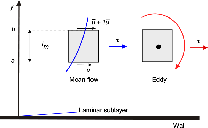
(47) $\begin{equation*} u' = \delta \overline{u} = l_m \frac{\partial \overline{u}}{\partial y} \end{equation*}$

The concept of the mixing length for a near-wall flow.

If it is also assumed that $u'$ and $v'$ are of the same order of magnitude, then turbulent shear stress is

(48) $\begin{equation*} \tau_t = - \varrho \, \overline{ u' v'} = \varrho \, l_m^2 \left|\frac{\partial u}{\partial y}\right| \frac{\partial u}{\partial y} \end{equation*}$

The simplest assumption for the mixing length, $l_m$ , is given by

(49) $\begin{equation*} l_m = k \, y \end{equation*}$

where $k$ is some constant. The mixing length can be considered the distance over which the fluid elements retain their original momentum as they move from one level to another within the turbulent boundary layer. Therefore, the eddy viscosity $\mu_t$ is given by

(50) $\begin{equation*} \mu_t = \varrho \, l_m^2 \left|\frac{\partial u}{\partial y}\right| \end{equation*}$

or in terms of the kinematic viscosity

(51) $\begin{equation*} \nu_t = l_m^2 \left| \frac{\partial u}{\partial y} \right| \end{equation*}$

The values of both of these latter parameters depend on the type and class of flow problem and are not known a priori, i.e., they are postdictive rather than predictive. Following the order of magnitude reduction approach done for laminar flows then, one form of the turbulent boundary layer equation is

(52) $\begin{eqnarray*} u \frac{\partial u}{\partial x} + v \frac{\partial u}{\partial y} & = & - \frac{1}{\varrho} \frac{\partial p}{\partial x} + (\nu+\nu_t) \frac{\partial^2 u}{\partial x^2} \\[8pt] \frac{\partial p}{\partial y} & = & 0 \label{two} \\[8pt] \frac{\partial u}{\partial x} + \frac{\partial v}{\partial y} & = & 0 \label{three} \end{eqnarray*}$

where the unknowns are $u$ and $v$ for a given pressure gradient $\partial p / \partial x$ and $\nu+\nu_t$ is the effective total kinematic viscosity. However, modeling turbulence in boundary layers is generally far more difficult because of its non-homogeneous and non-isotropic nature. Much of the past and current research work in turbulent boundary layer flows has to do with describing mathematically the nature of the turbulence.

Law of the Wall

The mixing length model leads to another model for the flow of a turbulent boundary layer called the law of the wall. This law has been proven for wall-bounded turbulent flows that develop in mild pressure gradients without flow separation. It helps to characterize and model the effects of turbulent flows near walls, which is crucial in many aerospace applications, such as in the design of airfoils, wings, and entire flight vehicles.

The law of the wall states that the velocity of a turbulent fluid flowing near a solid boundary exhibits a logarithmic relationship with the distance from the boundary. This type of relationship arises as a result of the complex interactions between the fluid and the boundary, which result in turbulent fluctuations in velocity, a result verified by experiments. Mathematically, the law of the wall, which is an empirical construct, can be expressed as

(53) $\begin{equation*} \dfrac{1}{{\cal{K}}} \ln(y_+) + B \end{equation*}$

as shown in the figure below in terms of $u_+$ and $y_+$ , which are dimensionless parameters called wall units. This is a classic presentation in the field of boundary layers, although initially perhaps somewhat nonintuitive. Nevertheless, this is one of the most famous empirically determined relationships for turbulent flows over solid boundaries.

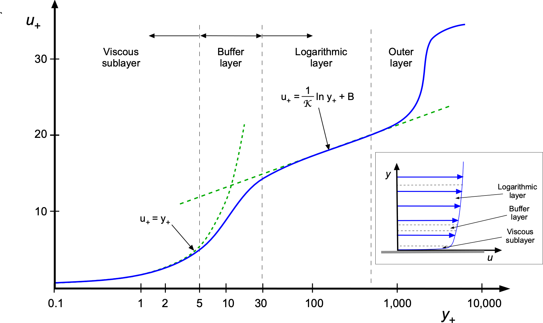
The “law of the wall” describing the turbulent boundary layer over a solid surface is an accepted and valuable concept in aerodynamics.

The value of $u_+$ is a dimensionless velocity, defined as $u/u_*$ , where $u$ is the velocity of the fluid and $u_*$ is the so-called friction velocity, $u_*$ . Because the shear stress on the wall, $\tau_w$ , is

(54) $\begin{equation*} \tau_w = \varrho u_*^2 \end{equation*}$

then, the friction velocity is defined by

(55) $\begin{equation*} u_* = \sqrt{ \dfrac{\tau_w}{\varrho}} \end{equation*}$

which is just an alternative measure of the shear stress. The value of $y_+$ is defined as

(56) $\begin{equation*} y_+= \dfrac{u_* \, y}{\nu} \end{equation*}$

where $y$ is the distance from the wall and $\nu$ is the kinematic viscosity of the fluid. It will be apparent that the value of $y_+$ is effectively a Reynolds number, so it becomes a measure of the relative importance of inertial or turbulent transport effects in the flow to the viscous effects as a function of the distance away from the wall. In this regard, a presentation of $u_+$ versus $y_+$ now becomes more meaningful.

The laminar sublayer model is valid for $y_+ < 5$ . However, this value can vary between 10 and 3, depending on the flow. The transition or the “buffer layer” occurs for $5 \le y_+ \le 30$ . The logarithmic profile is valid further away in the outer layer where the flow is turbulent. The parameter ${\cal{K}}$ is known as the von Kármán constant, which has an accepted empirical value of 0.41. However, this value could change as higher fidelity measurements in turbulent boundary layers become available. Finally, the value of $B$ is a constant that depends on the particular flow configuration and external boundary conditions, which must also be derived empirically. Although semi-empirical, the law of the wall provides a valuable mathematical framework for understanding and predicting the effects of turbulent flows near solid boundaries.

Notice that the values of $u_+$ and $y_+$ depend on a knowledge of the wall stress, $\tau_w$ . There are various ways of measuring and calculating $\tau_w$ . If the flow velocities near the wall are available, then a direct approach would be to calculate the velocity gradient. However, to do this with CFD requires a very fine grid near the wall, which may not be possible because of grid size or computational limitations. Likewise, it can be challenging with experiments to make enough flow velocity measurements very close to a surface to determine a gradient. Alternatively, indirect methods, such as a Stanton tube, Preston tube, or hot-film sensor, can be used to determine shear stress through calibration.

There’s turbulence in my coffee!

When you pour milk into a cup of coffee, the collisions between the descending milk stream and the rising coffee create turbulence that helps mix the milk and coffee more effectively and enhances the release of aromatic compounds.

Stirring with a spoon creates an eddy the size of the cup. This large eddy generates smaller eddies that, in turn, generate even smaller ones, and so on. Turbulence can also lead to the introduction of air into the liquid, creating a layer of microfoam on the surface. The heat exchange between the hot coffee and the cooler milk helps equalize temperatures more rapidly.

Turbulence Models

The Boussinesq hypothesis is commonly used in developing turbulence models for solving the RANS equations to determine the value of $\mu_t$ . These models can be utilized to simulate turbulent flows in practical engineering applications. This hypothesis provides a simple and computationally efficient way to incorporate the effects of turbulence into the Navier-Stokes equations, allowing for the prediction of the mean flow behavior and turbulence statistics. However, it must be recognized that the Boussinesq hypothesis is just an approximation of turbulent flows, including that they are isotropic (i.e., the properties are the same in all spatial dimensions) and homogeneous (i.e., uniformly mixed).

In more complex turbulent flows, the Boussinesq hypothesis may need to be modified or replaced by more advanced turbulence models, especially considering turbulence is often anisotropic. Various turbulence models are available to determine $\mu_t$ , each with its own assumptions and levels of complexity. Some commonly used turbulence models in RANS simulations include:

The Spalart-Allmaras (SA) turbulence model is a one-equation model that directly solves for the eddy viscosity. It is known for its simplicity and efficiency and is widely used, especially as a benchmark.
k-epsilon or $k$ – $\epsilon$ models solve for two transport equations, one for the turbulent kinetic energy $k$ and another for the turbulent dissipation rate $\epsilon$ . Variations of this model include the RNG $k$ – $\epsilon$ and Realizable $k$ – $\epsilon$ .
k-omega or $k$ – $\omega$ models also solve for two equations but use different variables, turbulent kinetic energy $k$ and specific dissipation rate $\omega$ . Variations include the SST $k$ – $\omega$ and BSL $k$ – $\omega$ models.
Reynolds Stress Models (RSM) resolve the Reynolds stresses directly, providing more detailed information about the turbulence field. They are designed for application to flows with anisotropic turbulence, flow separation, and recirculation. However, RSM is computationally more expensive than other models.

In addition, two other methods of solving the Navier-Stokes equations are worth mentioning, namely LES and DNS.

Large Eddy Simulation (LES) is not a RANS model but is worth mentioning. LES focuses on capturing the larger, energy-containing eddies while modeling the effects of the smaller, dissipative eddies. It is a computationally expensive method but provides more accurate results for complex flows.
DNS stands for Direct Numerical Simulation, a computational technique used in fluid dynamics to simulate turbulent flows. In DNS, all the scales of motion in a turbulent flow are resolved numerically without any turbulence modeling. This means that even the smallest eddies and fluctuations in the flow are explicitly simulated. However, these simulations are limited to elementary geometries and small geometric scales.

The engineer’s choice of turbulence model depends on the specific characteristics of the simulated flow, the available computational resources, and the desired level of accuracy. However, the lack of generality of such models to all types of flows limits the ability to predict turbulent flow properties, especially the development of turbulent boundary layers. Developing better turbulence models is still a goal in modern fluid dynamics, although these models are considered postdictive (i.e., after the fact) rather than predictive. It is common for engineers and researchers to perform sensitivity analyses using different turbulence models to assess the impact on simulation results and to compare them to benchmark solutions if available. These benchmarks may include both experiments and other theories.

Numerical Solution of the RANS Equations

Solving RANS equations numerically involves discretizing the governing equations into a set of algebraic equations that can be solved on a computer. The RANS equations consist of the continuity and momentum equations, typically solved using finite volume or finite difference methods.

As shown below, the first step is to divide the computational domain into a fine grid (or mesh) of finite volumes or cells for a lifting surface. The Navier-Stokes equations are then discretized over these cells using numerical methods. The numerical method must also be discretized into time steps to resolve the temporal evolution of the flow.

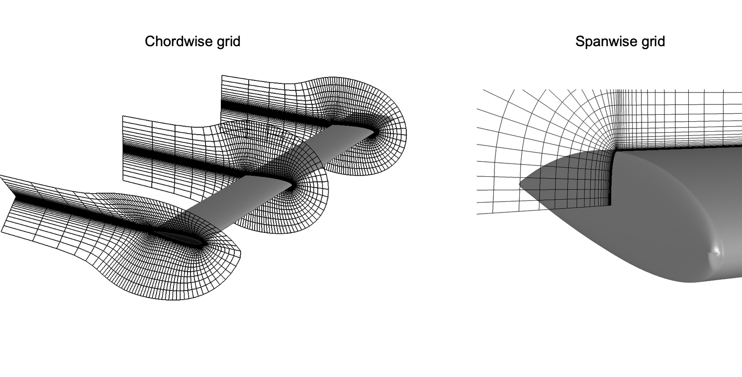
Examples of computational grids used to solve for the flow about a wing.
Apply the conservation equations (continuity and momentum) to each control volume. This involves discretizing the spatial and temporal derivatives in the equations. Typical schemes for solving the equations for the flow velocities and pressures include explicit and implicit time-stepping methods.
The resulting discretized equations form a system of linear algebraic equations. This system is solved iteratively at each time step until convergence is achieved. Implicit methods involve solving a system of equations at each time step, while explicit methods update the solution based on the current values.
Implement the selected turbulence model within the selected numerical framework. This step involves solving additional equations for turbulence quantities, such as a turbulence closure model.
Apply appropriate boundary conditions to represent the physical boundaries of the problem. This may include specifying inlet, wall, and outlet conditions.
Iterate through the time steps until a steady state or a time-accurate solution is reached. Monitor convergence criteria and adjust the solution until the changes between iterations are within acceptable tolerances or other criteria.
Analyze and post-process the numerical results to extract relevant information such as velocity profiles, pressure distributions, Reynolds stresses, TKE, and other turbulence quantities. The examples below show RANS predictions of the wing tip vortex rollup using two different turbulence models. Even though both solutions give similar bulk flow properties, different detailed quantitative properties and turbulence levels are obtained.

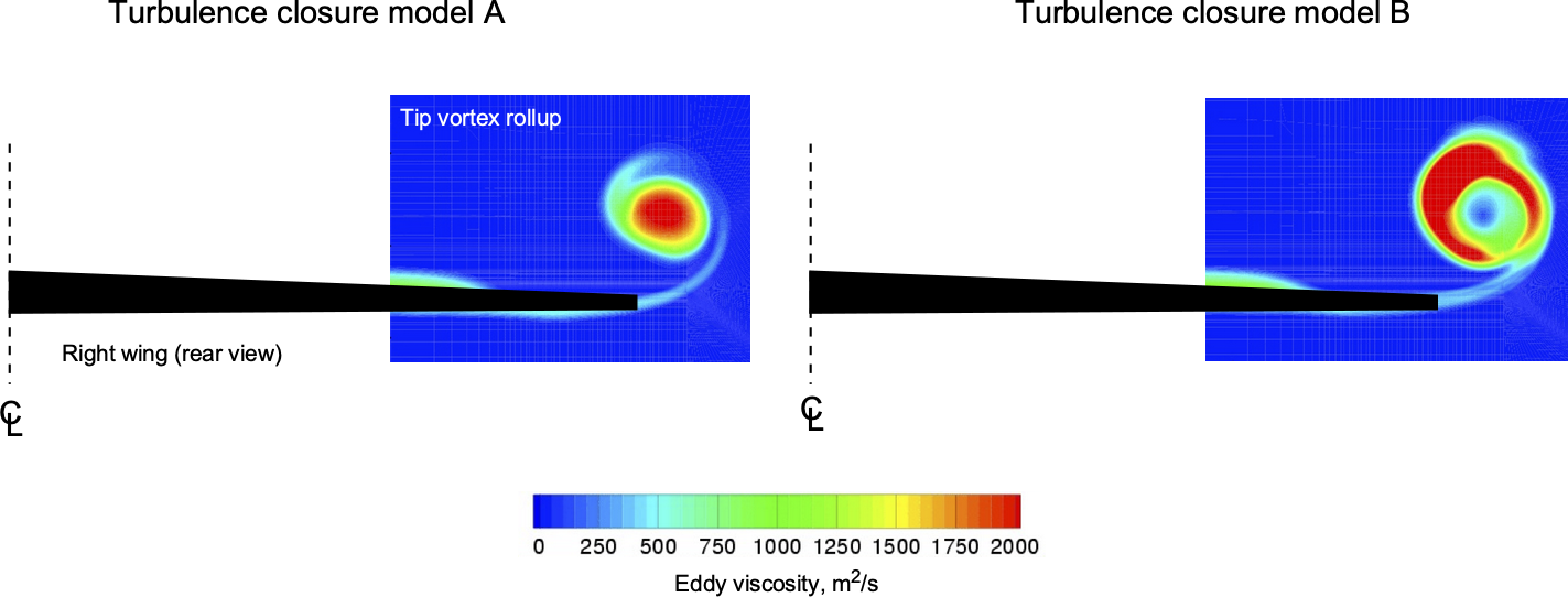
RANS predictions of the rollup and formation of the vortex at the tip of a wing using two different turbulence models. The differences may have to be reconciled with reference to experiments.

Numerical solvers for RANS equations can be found in various computational fluid dynamics (CFD) software packages. They often include pre-processing tools for mesh generation, turbulence model setup, and post-processing tools for visualization and analysis of the results. The choice of numerical method and solver depends on factors such as the complexity of the flow, computational resources, and desired outcomes in terms of resolution and accuracy. While the CFD prediction of the flow about an entire aircraft may still be beyond the state-of-the-art, as shown in the figure below, the confidence in such predictions is still 90% or better.

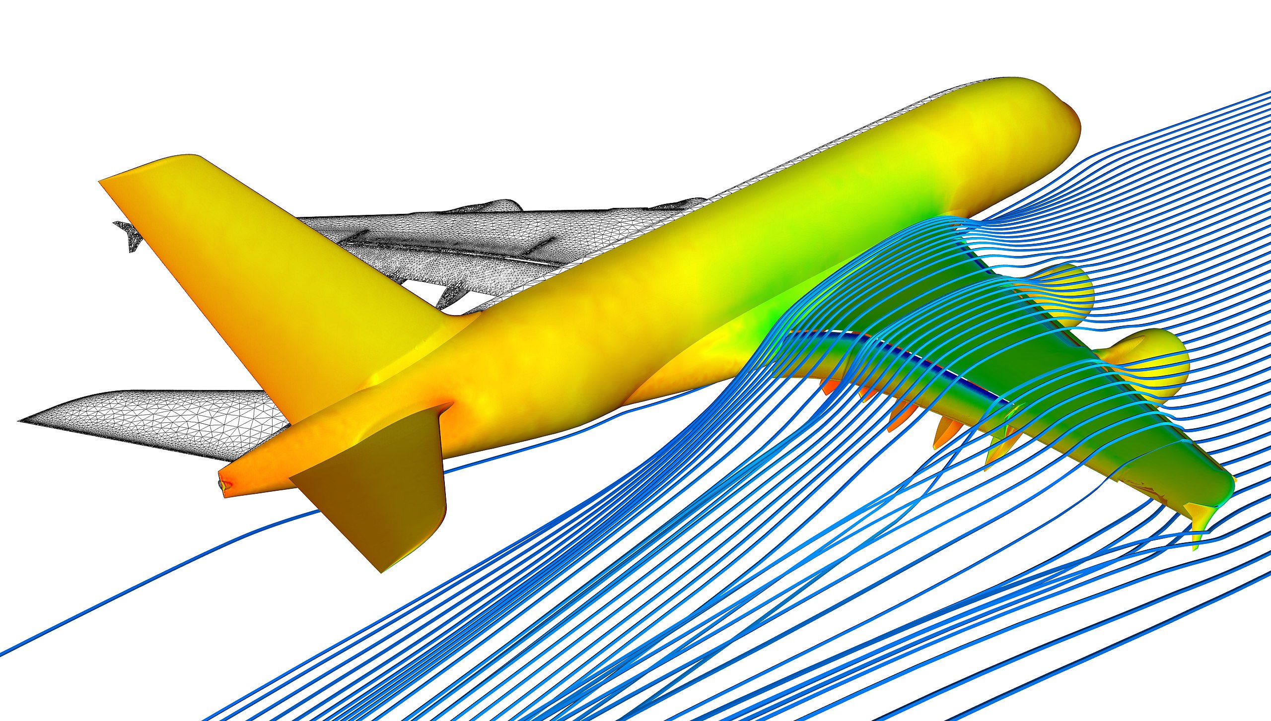
CFD solution for the flow about a complete aircraft.

Remember that the turbulence models used for CFD are postdictive, i.e., after-the-fact solutions, so they do not lead to any extra understanding of the mechanisms of turbulence. Solving the flow field numerically leads to irregular solutions that generally look like turbulence, but the outcomes are still an artifact of how mathematics is used to simulate turbulence. Nevertheless, remarkable details of the flows above complete aircraft can now be computed. In the end, however, all CFD solutions must be considered tentative and must be validated against experiments or another benchmark, one way or another.

Turbulence & Combustion

In many instances, turbulence is a desirable outcome in fluid dynamics, one being the combustion processes. In this regard, understanding fuel/oxidizer combustion processes in piston, jet, and rocket engines is essential. The creation of turbulence generates kinetic energy, forcing the mixing of fuel and oxidizer across various length scales. This turbulent mixing enhances the combustion rates and efficiency by increasing the interfacial area between reactants and promoting molecular collisions, mixing, and turbulence, as shown in the schematic below.

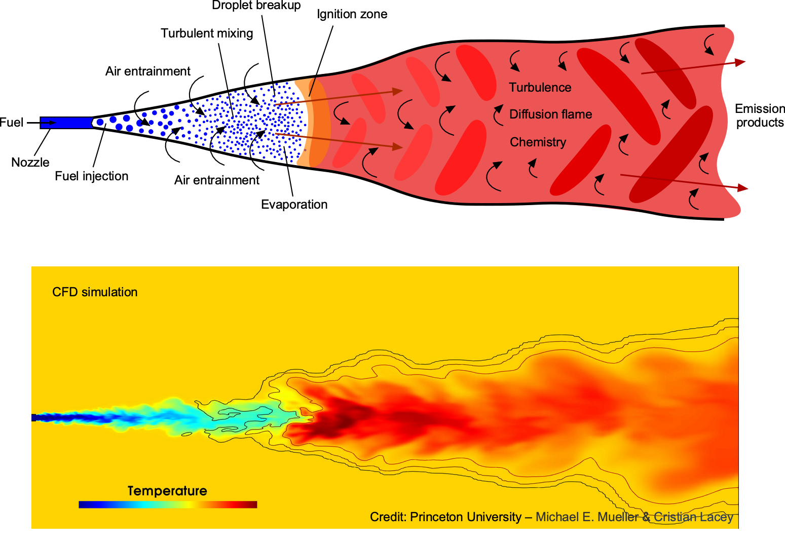
The combustion of a fuel and an oxidizer is a complex process, but the creation of turbulence and mixing plays a vital part in the efficiency of heat and energy production.

The interaction between turbulence and chemical reactions can also stabilize flame fronts and prevent combustion instabilities that may cause the engine to malfunction. Today, computational and experimental methods are employed synergistically to study turbulent combustion phenomena, aiding in developing advanced combustion systems that increase power and thrust generation while minimizing fuel consumption, i.e., reducing specific fuel consumption.

Reducing Turbulence

Turbulence intensity reductions can be achieved using “turbulence screens,” a staple in wind tunnel operations. These screens, also known as “anti-turbulence screens,” are made from fine wire mesh of various gages and grid spacings, as shown in the figure below. Positioned before the contraction to the test section, they break the larger turbulent eddies into progressively smaller ones that decay rapidly over short downstream distances. This process ensures a smoother and less turbulent flow in the test section, a prerequisite for high-quality measurements. However, it is important to note that the screens themselves may also introduce some small-scale turbulence, depending on the Reynolds number of the wires.

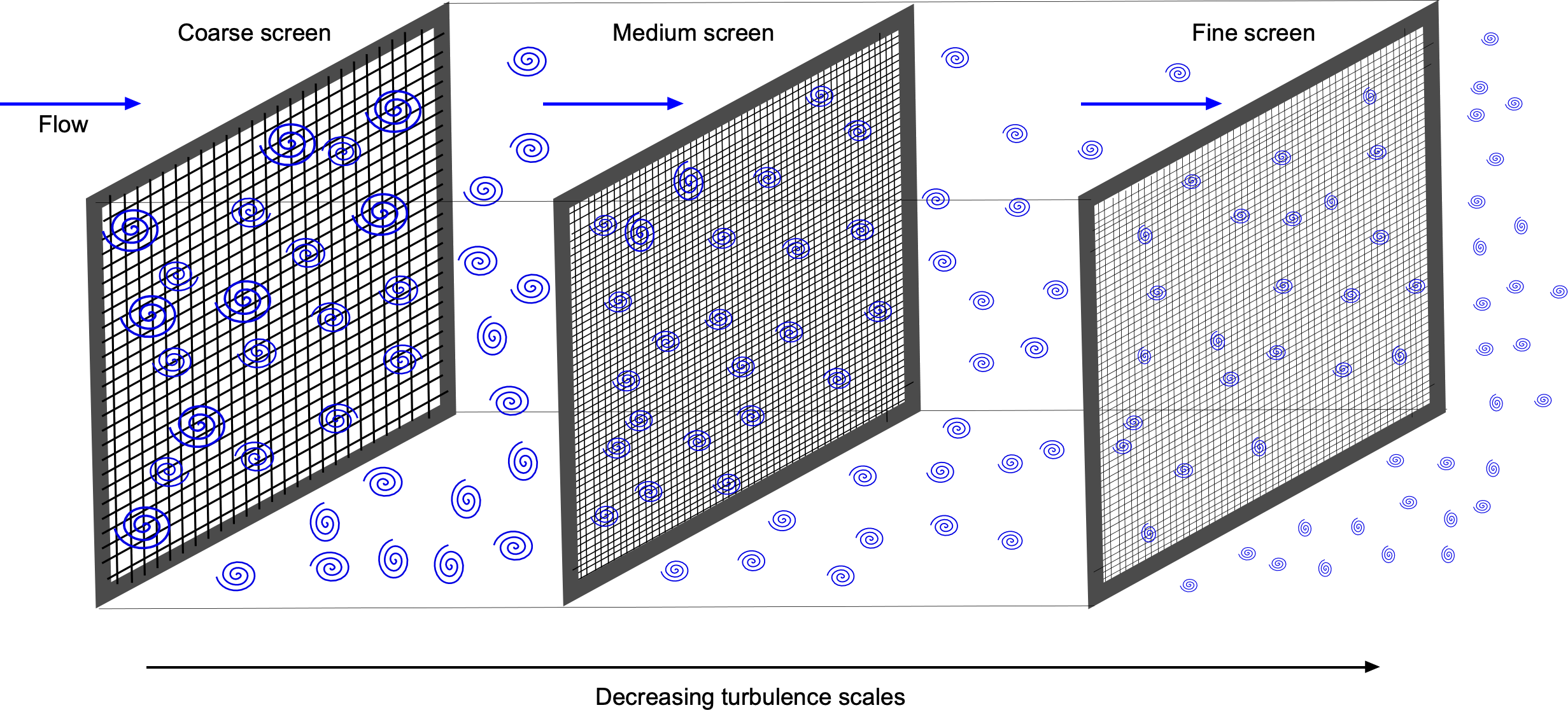
A “settling chamber” downstream of the last turbulence screen reduces the turbulence further and also allows it to reach an equilibrium state with more homogeneous turbulence levels. As the flow passes through a contraction section, the remaining turbulence is effectively squeezed out, and the flow entering the test section becomes almost laminar, but not entirely. Turbulence levels of less than 0.1% of the free-stream velocity are considered good enough to represent the flow in the higher atmosphere.

Summary & Closure

A turbulent flow, by definition, is an unsteady flow because the fluid properties at a given point in the flow continuously change over time. This behavior contrasts with a smooth, laminar flow, where the fluid moves in layers with minimal mixing. Turbulent flows are more complex and challenging to analyze than laminar flows, requiring alternative mathematical models and computational methods. In aerospace engineering, turbulent flows constitute a fundamental behavior that significantly influences the performance of all flight vehicles. Turbulence is characterized by random flow velocity and pressure fluctuations. Therefore, it poses a significant challenge for engineers to understand and model as it might affect the performance and characteristics of flight vehicles. In particular, the intricate interplay of Reynolds stresses vorticity generation and flow separation requires further understanding to mitigate adverse effects.

Mathematical models like the Navier-Stokes equations can be used to describe turbulent flows. However, solving these equations accurately for all turbulence scales remains challenging. Engineers can employ advanced computational fluid dynamics (CFD) simulations in conjunction with wind tunnel testing to comprehend and predict the effects of turbulence on the aerodynamics of flight vehicles. However, because of the complex, nondeterministic nature of turbulence, CFD simulations such as RANS and experiments must be undertaken synergistically to study and analyze turbulent flows. It is essential to choose an appropriate turbulence model based on the specific characteristics of the flow, as well as the computational resources available. Different turbulence models have their strengths and limitations, and the choice depends on factors such as the flow conditions, the geometry about which the flow developed, and the desired level of accuracy. What is clear, however, is that continuing to understand the complex characteristics of turbulence is essential for optimizing future aircraft designs and improving fuel efficiency.

5-Question Self-Assessment Quickquiz

For Further Thought or Discussion

Research examples of natural phenomena where turbulence may play a significant role.
Discuss the importance of understanding turbulence in aerodynamics and aircraft design.
What are the challenges in predicting and modeling turbulence?
How might turbulence affect heat transfer in various applications?
Why does the Reynolds number affect the onset and development of turbulent flow?
Have there been any engineering technologies that have been specifically developed to harness turbulence?

Other Useful Online Resources

To learn more about turbulent flows, take a look at some of these online resources:

Video on understanding laminar and turbulent flows.
Turbulent flows are MORE awesome than laminar flows.
Great flow visualization on the transition from laminar to turbulent flow – repeating Reynolds’s experiment.
What is turbulence? Turbulent fluid dynamics are everywhere!

However, modern physicists have minimal interest in turbulence over subjects like quantum mechanics. ↵
It is not quite a literal translation from Da Vinci's unique Latin form, but it is close enough. ↵

License

Icon for the Creative Commons Attribution-NonCommercial-NoDerivatives 4.0 International License

Introduction to Aerospace Flight Vehicles Copyright © 2022, 2023, 2024 by J. Gordon Leishman is licensed under a Creative Commons Attribution-NonCommercial-NoDerivatives 4.0 International License, except where otherwise noted.