Energy Equation & Bernoulli’s Equation

J. Gordon Leishman

doi:https://doi.org/10.15394/eaglepub.2022.1066.n18

22 Energy Equation & Bernoulli’s Equation

Introduction

Energy is defined as the ability to do work, which is a beneficial descriptive physical property in science and engineering. There are many types of energy, including potential, kinetic, chemical, electrical, and nuclear energy. For thermodynamic analyses, energy can be classified into two categories: macroscopic energy and microscopic energy. Macroscopic energy is the energy that a whole system possesses with respect to a fixed external reference, and in thermodynamics, this includes both potential and kinetic energies. Microscopic energy refers to the energy contained within a system at the molecular level. A “system” in this context can be defined as a collection of matter of fixed identity.

When developing the energy equation for a fluid flow, the applicable physical principle is a thermodynamic one in that energy cannot be created or destroyed but only converted from one form to another. This principle is formally embodied in the first law of thermodynamics applied to a system of a given (fixed) mass, i.e.,

(1) $\begin{equation*} Q - W = \Delta E \end{equation*}$

where $Q$ is the change in the heat added to the system (such as from a thermal source), $W$ is the change in the work done on the system (such as mechanical work), and $\Delta E$ is the change in internal energy of the mass inside that system. Notice that $Q$ is positive when heat is added to the system and negative when heat is lost. Likewise, $W$ is positive when work is done on the system and negative when the system does work on the fluid.

Internal energy can be considered the sum of the macroscopic kinetic and potential energies of the molecules comprising the fluid, as well as their microscopic internal energy, such as temperature effects. Indeed, when dealing with thermodynamic relations, the internal energy of a perfect gas is a function of temperature alone. Therefore, another way of writing the first law of thermodynamics for a fixed system is

(2) $\begin{equation*} ( Q_{\rm in} - Q_{\rm out} ) + ( W_{\rm in} - W_{\rm out} ) = \Delta E \end{equation*}$

as shown in the figure below.

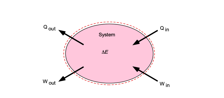
The first law of thermodynamics states that the change in internal energy of a fixed system is equal to the net heat added minus the net work done on that system.

If the system does no external work, all the heat added will manifest as an increase in internal energy, e.g., an increase in temperature. Of course, heat and work can be added to or subtracted from an engineering system, i.e., transferred across the system’s boundaries. If $Q$ is the heat added, and $W$ is the work done, then the conservation of energy in this differential form can be written as

(3) $\begin{equation*} \underbrace{ \frac{\partial Q}{\partial t}}_{\begin{tabular}{c} \scriptsize Time rate of \\[-3pt] \scriptsize change of heat \\[-3pt] \scriptsize into the system.\end{tabular}} + \underbrace{ \frac{\partial W}{ \partial t}}_{\begin{tabular}{c} \scriptsize Time rate of \\[-3pt] \scriptsize change of work \\[-3pt] \scriptsize into the system.\end{tabular}} = \underbrace{ \frac{dE}{dt}}_{\begin{tabular}{c} \scriptsize Time rate of \\[-3pt] \scriptsize change of energy \\[-3pt] \scriptsize inside the system.\end{tabular}} \end{equation*}$

By convention, heat added to the system and the rate of work done on the system are defined as positive contributions. The system’s energy can also be viewed as being associated with that system’s specific amount of mass. Therefore, for a fluid flow, the energy terms in the resulting equations are usually written as an energy per unit mass, i.e., in the spirit of the differential calculus, then

(4) $\begin{equation*} \frac{\partial q}{\partial t} + \frac{\partial w}{ \partial t} = \frac{de}{dt} \end{equation*}$

This latter approach is also consistent with the previous derivations of the equations that applied to the conservation of mass and momentum.

Learning Objectives

Set up the most general form of the energy equation in integral form.
Know how to simplify the energy equation into various, more practical forms.
Understand how to derive a surrogate for the energy equation for steady, incompressible, inviscid flow, called the Bernoulli equation.
Learn how to solve fundamental engineering problems using the energy equation.

Setting Up the Energy Equation

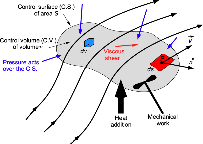
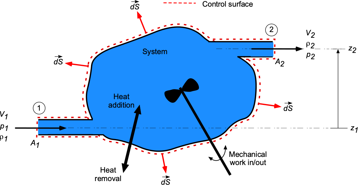
As before, regarding the development of the equations governing the conservation of mass and momentum, consider a fluid flow through a fixed finite control volume (C.V.) of volume ${\cal {V}}$ , bounded by a control surface (C.S.) of area, $S$ , as shown in the figure below. The flow velocity is $\vec{V}$ at any point inside the C.V. or on the C.S. At a point on the C.S., the unit normal, $\vec{{n}}$ , and the unit normal vector area, $d\vec{S}$ , can be defined. Also, let $d{\cal {V}}$ be an elemental fluid volume inside the C.V., which will contain a fluid of elemental mass $\varrho \, d{\cal {V}}$ .

A finite control volume fixed in space as used to establish the energy equation in its most general form.

The objective is to develop an analogous equation to the continuity and momentum equations for energy conservation as they apply to a fluid flow. As will be shown, however, the resulting energy equation describes a power balance equation for the fluid system, i.e., a balance of the rate of work done on the flow versus the rate of energy added to the flow and/or conversion from one form of energy in the flow to another.

Heat Addition

An increment in energy, ${de}$ , can be added to the elemental fluid volume $d{\cal{V}}$ in the form of heat, $dq$ , so that $de = dq$ . Heat energy can be added (or subtracted) by conduction, convection, or radiation, e.g., because of a temperature difference. However, heat energy is often added to a system through combustion, e.g., the liberation of heat energy from stored chemical energy in a fuel. Therefore, the rate of volumetric heat addition will be

(5) $\begin{equation*} \mbox{Rate of volumetric heat addition to the C.V.} = \oiiint_{\rm C.V.} \overbigdot{q} \, \varrho \, d{\cal{V}} = \oiiint_{\cal{V}} \overbigdot{q} \, \varrho \, d{\cal{V}} \end{equation*}$

If the flow is viscous, then frictional effects can also add heat. This latter effect can be important on a high-speed (supersonic) aircraft or a spacecraft during re-entry into the Earth’s atmosphere. While viscous heating effects must be recognized as a complicated process involving the consideration of shear stresses and thermal effects from shock wave formation in a high-speed fluid flow, for now, the effects can be cumulatively denoted by $\overbigdot{Q}_{\mu}$ . Therefore, for the volume of fluid, then

(6) $\begin{equation*} \mbox{Total rate of heat addition to C.V.} = \oiiint_{\rm C.V.} \overbigdot{q} \, \varrho \, d {\cal{V}} + \overbigdot{Q}_{\mu} = \oiiint_{\cal{V}} \overbigdot{q} \, \varrho \, d {\cal{V}} + \overbigdot{Q}_{\mu} \end{equation*}$

Alert: Symbol conflict!

Symbol conflict is common between branches of engineering. In the situation just examined, $Q$ is used for heat, and $\overbigdot{Q}$ means the rate of heat addition. In other contexts, $Q$ can also mean volume flow rate. It is essential to avoid such conflicts, which can be done by redefining a new symbol. For example, the volume flow rate can be defined as ${\overbigdot{{\cal{V}}}}$ to avoid any ambiguity.

Work

If some work is done on the system, i.e., $dw$ per unit mass, the system’s energy will increase further. Work can be done by the effects of forces resulting from the action of pressure, body forces, viscous shear, and/or mechanical work. Remember that work is equivalent to a force times a distance, and power is the rate of doing work; therefore, power is equivalent to the product of a force and a velocity. In deriving the energy equation, one will notice that the terms have units of power, so the energy equation is a power equation.

In the case of pressure effects, a pressure force arises from the pressure acting over an area, i.e., for a point on the C.S. then $-p \, d\vec{S}$ , the minus sign indicating that the pressure force acts inward for an outward-pointing $d\vec{S}$ (by convention). Therefore, following the same type of process used for the derivation of the momentum equation, the work done by the pressure forces can be expressed as

(7) $\begin{equation*} \mbox{Rate of doing work on the C.S. by pressure forces} = -\oiint_{\rm C.S.} (p \, d\vec{S}) \bigcdot \vec{V} = -\oiint_{S} (p \, d\vec{S}) \bigcdot \vec{V} \end{equation*}$

Similarly, the effects of body forces can be written as

(8) $\begin{equation*} \mbox{Rate of doing work on the C.V. by body forces} = \oiiint_{\rm C.V.} ( \varrho \, \vec{f}_b \, d{\cal{V}} ) \bigcdot \vec{V} = \oiiint_{\cal{V}} ( \varrho \, \vec{f}_b \, d{\cal{V}} ) \bigcdot \vec{V} \end{equation*}$

In the case of viscous work, this latter contribution can be written as $\overbigdot{W}_{\mu}$ for the same reason as heat addition from viscous effects. This term is the rate of work done by viscous stresses acting on the C.S. over the C.S. If the viscous stresses are denoted by $\vec{\tau}$ , then

(9) $\begin{equation*} \mbox{Rate of doing work on the C.S. by viscous forces} = \oiiint_{\rm C.S.} \vec{\tau} \bigcdot d\vec{S} = \oiiint_{S} \vec{\tau} \bigcdot d\vec{S} = \overbigdot{W}_{\mu} \end{equation*}$

Finally, some mechanical work could be added to the system, say ${\overbigdot{W}_{\rm mech}}$ , an example being the work done by a pump. Work can also be extracted from a fluid flow, such as with a turbine, fan, or propeller. Therefore, adding all the contributions together gives

(10) $\begin{equation*} \mbox{Total rate of doing work} = -\oiint_{S} (p \, d\vec{S}) \bigcdot \vec{V} + \oiiint_{\cal{V}} ( \varrho \, \vec{f}_b \, d{\cal{V}} ) \bigcdot \vec{V} + \oiiint_{S} \vec{\tau} \, \bigcdot \, d\vec{S} + \overbigdot{W}_{\rm mech} \end{equation*}$

Internal Energy

The next step is to examine the internal energy within the C.V. Energy can do work, making this an important part of the energy equation. This form of energy will comprise some “temperature” energy or the microscopic kinetic energy per unit mass of the fluid molecules, ${e}$ , some macroscopic kinetic energy per unit mass of the fluid, $V^2/2$ , and some macroscopic potential energy per unit mass, $g z$ . In general, internal energy can be written as

(11) $\begin{equation*} \mbox{Energy per unit mass inside the C.V.} = e + \frac{V^2}{2} + g z \end{equation*}$

where the resultant velocity $V$ is obtained from $V^2 = u^2 + v^2 + w^2$ .

Notice that the microscopic energy of the fluid molecules, ${e}$ , can be considered as a sum of their translational kinetic, rotational, and vibrational energy, as suggested in the schematic below. The internal potential energy at the molecular level also contributes to total internal energy, e.g., molecular bonding, chemical, and nuclear energy. However, it is unnecessary to consider such latter effects at the present level of analysis. The best way of thinking about the internal energy of a fluid is in terms of its temperature.

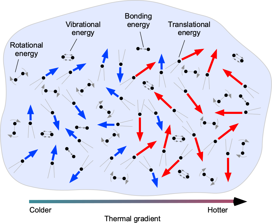The microscopic energy of the fluid molecules, ${e}$ per unit mass, can be considered as the sum of their translational energy, rotational energy, and vibrational energy.

The temperature of the fluid, $T$ , is proportional to the average total energy of the molecules, $E$ . This molecular relationship is usually written as $E = (3/2) k_B \, T$ , where ${k_B}$ is known as Boltzmann’s constant. In this latter form, however, it strictly holds for monoatomic gases because they have three degrees of translational freedom, i.e., kinetic energy only. A thermal gradient, for example, causes the molecules to move faster toward higher temperatures. Thermal energy will be transferred from the hotter part of the gas to the cooler part, basically a statement of the second law of thermodynamics, i.e., energy flows “downhill” toward a thermodynamic equilibrium.

Diatomic gases, such as nitrogen and oxygen, which comprise approximately 98% of air, also exhibit two degrees of rotational motion and two degrees of vibrational motion, the latter being significant only at higher temperatures. Therefore, their total internal energy will be related using $E = (5/2) k_B \, T$ at lower temperatures and $E = (7/2) k_B \, T$ at higher temperatures.

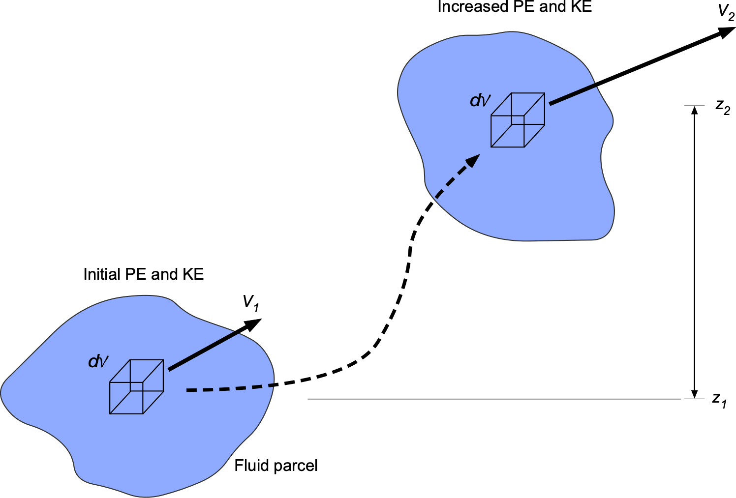
The macroscopic kinetic energy per unit mass of the fluid per unit mass, $V^2/2$ , and potential energy per unit mass, $g z$ , can be interpreted within the framework of a continuum model, as shown in the schematic below. Increasing the velocity of the fluid volume or parcel increases its bulk kinetic energy, and increasing the height of the fluid or its pressure “head” increases its bulk potential energy. Some work on the fluid must be done to increase either, which also requires energy.

The macroscopic kinetic and potential energy of the fluid can be interpreted within the framework of a continuum model.

Energy In & Out of Control Volume

The total energy will then be obtained by integration over the entire mass of fluid contained within the C.V., remembering that mass can also flow across the C.S. from the C.V. Across the element $dS$ , the mass flow rate will be $\varrho \, \vec{V} \bigcdot d\vec{S}$ . Therefore, the total energy flow rate across the entire surface of the C.V. then follows by integration, i.e.,

(12) $\begin{equation*} \mbox{Net flow of energy across the C.S.} = \oiint_{\rm C.S.} (\varrho \, \vec{V} \bigcdot d\vec{S}) \left( e + \frac{V^2}{2} + g z\right) = \oiint_{S} (\varrho \, \vec{V} \bigcdot d\vec{S}) \left( e + \frac{V^2}{2} + g z\right) \end{equation*}$

In addition, unsteady effects may be present so that the energy in the system can change because of temporal variations of the flow field properties inside $\cal{V}$ . For this contribution, then, the total energy inside the C.V. is

(13) $\begin{equation*} \mbox{Total energy inside the C.V.} = \oiiint_{\rm C.V.} \varrho \left( e + \frac{V^2}{2} + g z\right) d{\cal{V}} = \oiiint_{\cal{V}} \varrho \left( e + \frac{V^2}{2} + g z\right) d{\cal{V}} \end{equation*}$

and so the time rate of change of energy inside the C.V. will be

(14) $\begin{equation*} \text{Time rate of change of energy inside C.V.} = \frac{\partial}{\partial t} \oiiint_{\rm C.V.} \varrho \left( e + \frac{V^2}{2} + g z\right) d{\cal{V}} = \frac{\partial}{\partial t} \oiiint_{\cal{V}} \varrho \left( e + \frac{V^2}{2} + g z\right) d{\cal{V}} \end{equation*}$

Finally, adding these two latter terms together (Eqs. 12 and 14) gives

(15) $\begin{equation*} \mbox{Total rate of change in energy} = \frac{\partial}{\partial t} \oiiint_{\cal{V}} \varrho \left( e + \frac{V^2}{2} + g z \right) d{\cal{V}} + \oiint_{S} (\varrho \, \vec{V} \bigcdot d\vec{S}) \left( e + \frac{V^2}{2} + g z \right) \end{equation*}$

Final Form of the Energy Equation

Now, all of the parts that make up the final form of the energy equation are available in its integral form. To this end, the principle of conservation of energy has been applied to a fluid flowing through a finite C.V. that may have heat added or removed, and/or mechanical work is done on the fluid or extracted from it, i.e.,

(16) $\begin{eqnarray*} \underbrace{\oiiint_{\cal{V}} \overbigdot{q} \, \varrho \, d {\cal{V}}}_{\begin{tabular}{c} \scriptsize Net flow rate\\[-3pt] \scriptsize of heat\\[-3pt] \scriptsize into C.V. \end{tabular}} & + & \underbrace{\overbigdot{Q}_{\mu}}_{\begin{tabular}{c} \scriptsize Rate of heat\\[-3pt] \scriptsize added into C.V. \\[-3pt] \scriptsize from viscous effects \end{tabular}} -\underbrace{ \oiint_{S} (p \, d\vec{S}) \bigcdot \vec{V}}_{\begin{tabular}{c} \scriptsize Work done \\[-3pt] \scriptsize on the C.S. by \\[-3pt] \scriptsize pressure forces \end{tabular}} \quad + \quad \underbrace{\oiiint_{\cal{V}} ( \varrho \, \vec{f}_b \, d{\cal{V}}) \bigcdot \vec{V}}_{\begin{tabular}{c} \scriptsize Work done \\[-3pt] \scriptsize on the C.V. by \\[-3pt] \scriptsize body forces \end{tabular}} \\[12pt] & & + \underbrace{\overbigdot{W}_{\mu}}_{\begin{tabular}{c} \scriptsize Work done \\[-3pt] \scriptsize on the C.V. \\[-3pt] \scriptsize by viscous forces \end{tabular}} + \underbrace{\overbigdot{W}_{\rm mech}}_{\begin{tabular}{c} \scriptsize Work done \\[-3pt] \scriptsize on the C.V. by \\[-3pt] \scriptsize mechanical sources \end{tabular}} \\[18pt] \hspace*{-200mm} = & \hspace*{-1mm} & \hspace*{-5mm} \underbrace{\frac{\partial}{\partial t} \oiiint_{\cal{V}} \varrho \left( e + \frac{V^2}{2} + g z\right) d{\cal{V}}}_{\begin{tabular}{c} \scriptsize Time rate of \\[-3pt] \scriptsize change of energy \\[-3pt] \scriptsize inside C.V. \end{tabular}} \quad + \quad \underbrace{\oiint_{S} (\varrho \, \vec{V} \bigcdot d\vec{S}) \left( e + \frac{V^2}{2} + g z\right) }_{\begin{tabular}{c} \scriptsize Net flow of energy \\[-3pt] \scriptsize out of C.V. per \\[-3pt] \scriptsize unit time \end{tabular}} \end{eqnarray*}$

which is mathematically the most general form of the energy equation.

Because energy is conserved, then in words, it can be stated that: “The rate of heat added plus the rate of doing work on the flow will be equal to the total rate of change of energy of the flow,” i.e.,

(17) $\begin{equation*} \Delta \overbigdot{Q} + \Delta \overbigdot{W} = \Delta \overbigdot{E} \end{equation*}$

which is just the first law of thermodynamics, where $\Delta Q$ is positive when heat is added to the system, and $\Delta W$ is positive when work is done on the system.

Rewriting the energy equation again, without the components being identified, gives

(18) $\begin{eqnarray*} \oiiint_{\cal{V}} \overbigdot{q} \, \varrho \, d {\cal{V}} + \overbigdot{Q}_{\mu} -\oiint_{S} (p \, d\vec{S}) \bigcdot \vec{V} + \oiiint_{\cal{V}} ( \varrho \, \vec{f}_b \, d{\cal{V}}) \bigcdot \vec{V} + \overbigdot{W}_{\mu} + \overbigdot{W}_{\rm mech} = & & \nonumber \\[8pt] \frac{\partial}{\partial t} \oiiint_{\cal{V}} \varrho \left( e + \frac{V^2}{2} + g z\right) d{\cal{V}} + \oiint_{S} (\varrho \, \vec{V} \bigcdot d\vec{S}) \left( e + \frac{V^2}{2} + g z\right) \end{eqnarray*}$

This latter equation (Eq. 18) now completes the set of three conservation equations, i.e., mass (continuity), momentum, and energy.

Recall, for completeness, that the continuity equation is

(19) $\begin{equation*} \underbrace{\frac{\partial}{\partial t}\oiiint_{\cal{V}} \varrho \, d {\cal{V}}}_{\begin{tabular}{c} \scriptsize Time rate of \\ [-3pt] \scriptsize change of mass \\[-3pt] \scriptsize inside C.V. \end{tabular}} + \underbrace{ \oiint_S \varrho \, \vec{V} \bigcdot d\vec{S}}_{\begin{tabular}{c} \scriptsize Net mass \\[-3pt] \scriptsize flow rate \\[-3pt] \scriptsize out of C.V. \end{tabular}} = 0 \end{equation*}$

and the momentum equation is

(20) $\begin{flalign*} \!\!\!\!\!\!\!\! \vec{F} = \underbrace{\oiiint_{\cal{V}} \varrho \, \vec{F} _b \, d{\cal{V}}}_{\begin{tabular}{c} \scriptsize Sum of \\[-3pt] \scriptsize body forces \\[-3pt] \scriptsize acting on C.V. \end{tabular}} - \!\!\!\!\! \underbrace{\oiint_S p \, d\vec{S}}_{\begin{tabular}{c} \scriptsize Sum of \\[-3pt] \scriptsize pressure forces \\[-3pt] \scriptsize acting on C.S. \end{tabular}} + \!\!\!\! \underbrace{ \vec{F}_{\mu}}_{\begin{tabular}{c} \scriptsize Sum of \\[-3pt] \scriptsize viscous forces \\[-3pt] \scriptsize acting on C.V. \end{tabular}} \!\!\!\!\!\! = \underbrace{ \frac{\partial}{\partial t}\oiiint_{\cal{V}} \varrho \, \vec{V} \, d {\cal{V}}}_{\begin{tabular}{c} \scriptsize Time rate of \\[-3pt] \scriptsize change of momentum \\[-3pt] \scriptsize inside C.V. \end{tabular}} + \underbrace{\oiint_S (\varrho \, \vec{V} \bigcdot d\vec{S}) \vec{V}}_{\begin{tabular}{c} \scriptsize Net flow of \\[-3pt] \scriptsize momentum \\ \scriptsize out of C.V. \\[-3pt] \scriptsize per unit time \end{tabular}} \end{flalign*}$

In such collective equations, the unknown parameters may include the velocities, pressures, densities, and temperatures, although not all quantities may be unknown or required in any given problem. A fourth equation is also available to round out the set, namely the equation of state $p = \varrho R T$ , which is “handy” because it reduces the number of unknown properties by one.

Simplifications of the Energy Equation

The general form of the energy equation in Eq. 18 may look somewhat forbidding, and it is if written out in its entirety. Nevertheless, as with the other conservation equations, the general form can be written in various simplified forms depending on the assumptions that might be made (and justified!), e.g., steady flow, absence of body forces, no heat added to the system, no mechanical work, no viscous forces, one-dimensional flow, etc. However, because thermodynamic principles are applied here, caution must be exercised when using the energy equation to ensure that all necessary terms are retained in all potential simplification processes. Remember that in engineering problem solving, any oversimplification of the governing equations without careful justification will likely result in disastrous predictive outcomes.

Single Stream System

To illustrate the steps involved in simplifying the energy equation, it is essential to recognize that many practical engineering problems involve fluid systems with a single inlet and a single outlet, where the mass flow rate through such a system is constant, and are sometimes referred to as single-stream systems. A general depiction of such a single-stream system is shown in the figure below, where some flow comes in at one side of the system and exits on the other. Notice that, in general, there could be a difference in the heights of the inlet and the outlet, so the gravitational potential energy or “head” terms must be retained.

For such a single-stream system, the general form of the energy equation can be reduced to the form

(21) $\begin{equation*} { \overbigdot{Q} + \overbigdot{W}_{\rm shaft} = \overbigdot{m} \left( (e_2 - e_1) + \frac{V_2^2 - V_1^2}{2} + g ( z_2 - z_1 ) + \left( \frac{p_2}{\varrho_2} - \frac{p_1}{\varrho_1} \right) \right) } \end{equation*}$

where the subscripts 1 and 2 refer to the inlet and outlet conditions, respectively.

Look carefully at Eq. 18 and consider how Eq. 21 is obtained. As you do that, remember that a mass flow rate or the “ $\overbigdot{m}$ term” is always viewed as the flow velocity times the density of the flow times the area through which the flow passes. Notice also the form of the pressure term. The rate of doing work by the pressure forces is equivalent to the product of the pressure times an area times a velocity, so the pressure term in Eq. 21 becomes equivalent to a net pressure contribution times the mass flow rate divided by density.

The left-hand side of the preceding equation represents the energy input, and the right-hand side represents the energy output. The energy input, in this case, comes from the rate of heat transfer to the fluid ${\overbigdot{Q}}$ , the rate of mechanical work being done on the fluid ${\overbigdot{W}_{\rm mech}}$ (such as through a shaft driven from outside of the system by a pump), as well as any work done by the pressure forces.

In such a system, the mass flow through the system is conserved (mass inside the system is constant if the flow is steady), so

(22) $\begin{equation*} \overbigdot{m} = \varrho_1 A_1 V_1 = \varrho_2 A_2 V_2 \end{equation*}$

Based on per unit mass, which means dividing the terms in the equations by $\overbigdot{m}$ , Eq. 21 becomes

(23) $\begin{equation*} q + w_{\rm shaft} = e_2 - e_1 + \frac{V_2^2 - V_1^2}{2} + g ( z_2 - z_1) + \left( \frac{p_2}{\varrho_2} - \frac{p_1}{\varrho_1} \right) \end{equation*}$

which is a common form of the steady flow energy balance in thermodynamics. Rearranging this equation gives

(24) $\begin{equation*} w_{\rm shaft} = \frac{V_2^2 - V_1^2}{2} + g ( z_2 - z_1 ) + \left( \frac{p_2}{\varrho_2} - \frac{p_1}{\varrho_1} \right) + ( e_2 - e_1 - q ) \end{equation*}$

The latter term in Eq. 24 can be viewed as the sum of the frictional losses, i.e., the value of $(e_2 - e_1 - q) > 0$ in accordance with the second law of thermodynamics. Such losses can be considered unavailable energy, most likely lost from a system as heat conduction, radiation, or viscosity.

Another way to write this previous equation is just

(25) $\begin{equation*} w_{\rm shaft} = \frac{V_2^2 - V_1^2}{2} + g ( z_2 - z_1 ) + \left( \frac{p_2}{\varrho_2} - \frac{p_1}{\varrho_1} \right) + \mbox{losses} \end{equation*}$

and with rearrangement, then

(26) $\begin{equation*} \frac{p_1}{\varrho_1} + \frac{V_1^2}{2} + g z_1 + w_{\rm shaft} = \frac{p_2}{\varrho_2} + \frac{V_2^2}{2} + g z_2 + \mbox{losses} \end{equation*}$

which is often referred to as the mechanical energy equation in terms of work per unit mass.

What are the units of Eq. 26? For this equation to be dimensionally homogeneous, the units of each of the terms must be the same, i.e.,

$\left[ \frac{p}{\varrho} \right] = \frac{ \rm M L T^{-2} (\rm L^{-2}) }{\rm M L^{3}} = \rm L^2 T^{-2}$

and

$\left[ \frac{V^2}{2} \right] = ( \rm L T^{-1})^2 = \rm L^2 T^{-2}$

and

$\left[ g z \right] = (\rm L T^{-2}) L = \rm L^2 T^{-2}$

Therefore, the equation is confirmed to be dimensionally homogeneous with units of L ${^{2}}$ T $^{-2}$ . Remember that work, $W$ , has units of $[W]$ = M L ${^{2}}$ T $^{-2}$ , therefore, units of L ${^{2}}$ T $^{-2}$ represent work per unit mass.

Particular Case: No Losses

The total energy must be conserved if the flow is ideal, with no irreversible processes such as turbulence, friction, or viscosity. Then the energy loss term $(e_2 - e_1 - q) \equiv 0$ , i.e., in that case, the internal energy does not change from frictional effects. Now, an even simpler form of the energy conservation equation is available, i.e.,

(27) $\begin{equation*} \frac{p_1}{\varrho_1} + \frac{V_1^2}{2} + g z_1 + w_{\rm shaft} = \frac{p_2}{\varrho_2} + \frac{V_2^2}{2} + g z_2 \end{equation*}$

or in terms of power, so bringing the $\overbigdot{m}$ back, gives

(28) $\begin{equation*} \overbigdot{m} \bigg( \frac{p_1}{\varrho_1} + \frac{V_1^2}{2} + g z_1 \bigg) + \overbigdot{W}_{\rm shaft} = \overbigdot{m} \bigg( \frac{p_2}{\varrho_2} + \frac{V_2^2}{2} + g z_2 \bigg) \end{equation*}$

Mechanical Work

Remember that when adding or subtracting mechanical work, $W_{\rm shaft}$ , to a flow is standard in aerospace thermodynamic systems, such as utilizing a pump, fan, turbine, or propeller, so that $W_{\rm shaft}$ can be positive or negative. The addition or subtraction of mechanical work to or from the system may appear as a change in the flow’s kinetic energy and/or the potential energy of the flow and/or the internal temperature and/or pressure in the system, or any combination.

In the case of a basic pump, which adds energy and does work on the fluid system, then

(29) $\begin{equation*} { \overbigdot{W}_{\rm shaft} = P_{p} } \end{equation*}$

where ${P_p}$ is the input power, and for the turbine, which takes energy and work from the fluid system to produce mechanical work and power output at a shaft, then

(30) $\begin{equation*} { -\overbigdot{W}_{\rm shaft} = P_{t} } \end{equation*}$

where $P_t$ is the output power. Therefore, another way of writing the energy equation is

(31) $\begin{equation*} \underbrace{ \overbigdot{m} \bigg( \frac{p_1}{\varrho_1} + \frac{V_1^2}{2} + g z_1 \bigg) }_{\begin{tabular}{c} \scriptsize Rate of energy \\[-3pt] \scriptsize entering C.V. \end{tabular}}+ \underbrace{ P_{p}}_{\begin{tabular}{c} \scriptsize Power added \\[-3pt] \scriptsize by pump \end{tabular}}= \underbrace{\overbigdot{m} \bigg( \frac{p_2}{\varrho_2} + \frac{V_2^2}{2} + g z_2 \bigg) }_{\begin{tabular}{c} \scriptsize Rate of energy\\[-3pt] \scriptsize leaving C.V. \end{tabular}} + \underbrace{ P_{t}}_{\begin{tabular}{c} \scriptsize Power subtracted \\[-3pt] \scriptsize by turbine \end{tabular}} \end{equation*}$

Finally, if the fluid is assumed to be incompressible, i.e., $\varrho_1 = \varrho_2 = \varrho$ , then

(32) $\begin{equation*} \overbigdot{m} \bigg( \frac{p_1}{\varrho} + \frac{V_1^2}{2} + g z_1 \bigg) + P_{p} = \overbigdot{m} \bigg( \frac{p_2}{\varrho} + \frac{V_2^2}{2} + g z_2 \bigg) + P_{t} \end{equation*}$

or in terms of per unit mass (again, divide by $\overbigdot{m}$ ), then

(33) $\begin{equation*} \frac{p_1}{\varrho} + \frac{V_1^2}{2} + g z_1 + {w}_{p} = \frac{p_2}{\varrho} + \frac{V_2^2}{2} + g z_2 + {w}_{t} \end{equation*}$

which is called the extended Bernoulli equation.

Energy Equation in Terms of “Head”

Civil and hydraulic engineers, who deal primarily with liquids rather than gases, often express the energy equation in terms of pressure head and specific weight. The pressure head or the static pressure head, ${h}$ , is the height of a liquid column corresponding to a particular pressure value, so that it will have units of length, i.e., meters or feet. After doing some problems with the energy equation, it will be apparent that using a pressure head is convenient.

Specific Weight

The specific weight is the weight of a unit volume of a fluid. The symbol ${\gamma}$ is often used to represent specific weight; however, this choice causes a symbol conflict with aerospace and mechanical engineers, who use ${\gamma}$ to represent the ratio of specific heats. Therefore, specific weight can be denoted by the symbol ${w}$ , i.e.,

(34) $\begin{equation*} w = \frac{\mbox{\small Weight~of~fluid}}{\mbox{\small Volume~of~fluid}} = \frac{ \varrho \, {\cal{V}} \, g}{{\cal{V}}} = \varrho \, g \end{equation*}$

or by rearrangement, then

(35) $\begin{equation*} \varrho = \frac{w}{g} \end{equation*}$

Using the specific weight, which can be obtained by dividing through Eq. 38 by $g$ , the incompressible energy equation in terms of the pressure head can be written as

(36) $\begin{equation*} \frac{p_1}{\varrho \, g} + \frac{V_1^2}{2g} + z_1 + {h}_{p} = \frac{p_2}{\varrho \, g} + \frac{V_2^2}{2g} + z_2 + {h}_{t} \end{equation*}$

or

(37) $\begin{equation*} \frac{p_1}{w} + \frac{V_1^2}{2g} + z_1 + {h}_{p} = \frac{p_2}{w} + \frac{V_2^2}{2g} + z_2 + {h}_{t} \end{equation*}$

where the units of all terms are now length (m or ft). If frictional losses are included, which can also be expressed in terms of head, i.e., ${h}_{l}$ , then

(38) $\begin{equation*} \frac{p_1}{w} + \frac{V_1^2}{2g} + z_1 + {h}_{p} = \frac{p_2}{w} + \frac{V_2^2}{2g} + z_2 + {h}_{t} + {h}_{l} \end{equation*}$

Pressure Head of a Pump or Turbine

The power, $P$ , of a pump or turbine can be expressed as

(39) $\begin{equation*} P = \overbigdot{m} \, g \, h \end{equation*}$

The mass flow rate, $\overbigdot{m}$ , is

(40) $\begin{equation*} \overbigdot{m} = \varrho \, {\overbigdot{{\cal{V}}}} \end{equation*}$

where ${\overbigdot{{\cal{V}}}}$ is the volume flow rate. Therefore,

(41) $\begin{equation*} P = w \, {\overbigdot{{\cal{V}}}} \, h \end{equation*}$

Of course, no pump or turbine can be 100% efficient, so if the efficiency is $\eta$ , then the power is

(42) $\begin{equation*} P = \frac{w \, {\overbigdot{{\cal{V}}}} \, h}{\eta} \end{equation*}$

Therefore, in the case of a pump (energy in) of power ${P_p}$ , then

(43) $\begin{equation*} h_p = \frac{ \eta_p \, P_p}{ w \, {\overbigdot{{\cal{V}}}}} \end{equation*}$

In the case of a turbine (energy out) of power $P_t$ , then

(44) $\begin{equation*} h_t = \frac{ \eta_t \, P_t}{ w \, {\overbigdot{{\cal{V}}}}} \end{equation*}$

Caution: Do not confuse the pressure head for a pump, $h_p$ , with horsepower units, denoted by “hp.” Conventionally, units are never italicized, so the distinction should be clear.

Check Your Understanding #1 – Using the energy equation to calculate pumping power

Apply conservation of energy principles to calculate the power required by a hydraulic pump to deliver fluid (oil) from one location to another. The pump is 75% efficient in converting mechanical input work to pressure. The inlet pressure, $p_1$ , is 100 kPa, and the outlet pressure, $p_2$ , is 500 kPa. The diameter of the inlet pipe, ${d_1}$ , is 10 cm, and the outlet pipe, ${d_2}$ , is 5 cm. The flow rate, ${\overbigdot{{\cal{V}}}}$ , is 60 m³/hr. The height difference, $z_2 - z_1$ , is 3.2 m. The density of the hydraulic fluid is 850 kg/m³. Assume the internal fluid losses are equivalent to 1.4 m of static pressure head.

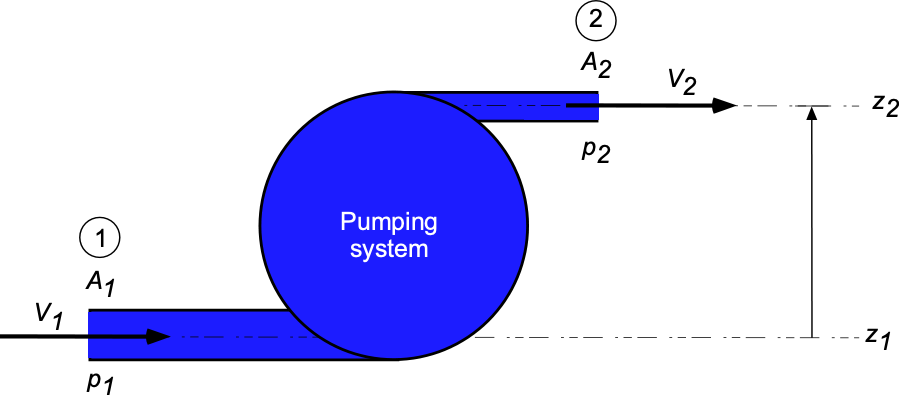
Show solution/hide solution.

First, it is necessary to find the inlet and outlet velocities, ${V_1}$ and ${V_2}$ , respectively, i.e.,

$V_1 = \frac{\overbigdot{{\cal{V}}}}{A_1} = \frac{4 {\overbigdot{{\cal{V}}}}}{\pi d_1^2} = \frac{4 \times 60.0/3,600}{\pi \times 0.1^2} =2.12~\mbox{m/s}$

and for ${V_2}$ , then

$V_1 = \frac{\overbigdot{{\cal{V}}}}{A_2} = \frac{4 {\overbigdot{{\cal{V}}}}}{\pi d_2^2} = \frac{4 \times 60.0/3,600}{\pi \times 0.05^2} =8.49~\mbox{m/s}$

The relevant form of the energy equation is

$\frac{p_1}{\varrho \, g} + \frac{V_1^2}{2g} + z_1 + {h}_{p} = \frac{p_2}{\varrho \, g} + \frac{V_2^2}{2g} + z_2 + h_l$

So, solving for $h_p$ gives

$h_{p} = \frac{p_2 - p_1}{\varrho \, g} + \frac{V_2^2 - V_1^2}{2g} + (z_2 - z_1) + h_l$

Inserting the known values gives

$h_{p} = \frac{(500.0 - 100.0) \times 10^3}{850.0 \times 9.81} + \frac{8.49^2 - 2.12^2}{2.0 \times 9.81} + 3.2 + 1.4 = 56.15~\mbox{m}$

The power required from the pump is

$P_p = \frac{ \varrho \, g \, {\overbigdot{{\cal{V}}}} \, h_p}{\eta_p}$

Inserting the numerical values gives

$P_p = \frac{ 850.0 \times 9.81 \times (60.0/3,600) \times 56.15}{0.75} = 10.41 ~\mbox{kW}$

Bernoulli’s Equation

By assuming incompressible flow and that no mechanical work is introduced into or taken out of the fluid system, then ${w}_{p} = {w}_{t} = 0$ , and so Eq. 38 becomes

(45) $\begin{equation*} \frac{p_1}{\varrho} + \frac{V_1^2}{2} + g z_1 = \frac{p_2}{\varrho} + \frac{V_2^2}{2} + g z_2 \end{equation*}$

This latter equation can then be rearranged into the form

(46) $\begin{equation*} p_1 + \frac{1}{2} \varrho V_1^2 + \varrho g z_1 = p_2 + \frac{1}{2} \varrho V_2^2 + \varrho g z_2 \end{equation*}$

or simply that

(47) $\begin{equation*} p + \frac{1}{2} \varrho \, V^2 + \varrho g z = \mbox{constant} \end{equation*}$

which is known as the Bernoulli equation or Bernoulli’s principle after Daniel Bernoulli.

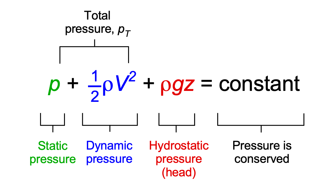
Note that the Bernoulli equation has units of pressure, not energy. For this reason, the Bernoulli equation is often referred to as a surrogate for the energy under the conditions of steady, incompressible flow without energy addition. It will be apparent that the Bernoulli equation remains a statement of energy conservation, as a fluid exchanges kinetic energy for pressure, either static or potential, with the specific kinetic energy being the kinetic energy per unit volume, as illustrated in the figure below. Notice that the sum of the static and dynamic pressures is referred to as the total pressure.

The terms in the Bernoulli equation are static, dynamic, and hydrostatic pressure, which are conserved.

A more general form of the Bernoulli equation, which often appears in many sources, is to leave it in an unintegrated form, i.e.

(48) $\begin{equation*} { \frac{dp}{\varrho} + \frac{1}{2} d( V^2 ) + g z = 0 } \end{equation*}$

After integration then

(49) $\begin{equation*} \int \frac{dp}{\varrho} + \frac{1}{2} V^2 + g z = \mbox{constant} \end{equation*}$

Assuming incompressible flow gives

(50) $\begin{equation*} \frac{p}{\varrho} + \frac{1}{2} V^2 + g z = \mbox{constant} \end{equation*}$

or

(51) $\begin{equation*} p + \frac{1}{2} \varrho \, V^2 + \varrho g z = \mbox{constant} \end{equation*}$

as has been written down previously.

The Bernoulli equation is one of the most famous equations in fluid mechanics, and it can be used to solve numerous practical problems. It has been derived here as a particular degenerate case of the general energy equation for a steady, inviscid, incompressible flow. Still, it can also be derived in several other ways. Remember that it is not an energy equation per se, as it has units of pressure; therefore, it is often referred to as a surrogate for the energy equation.

Another Derivation of Bernoulli’s Equation

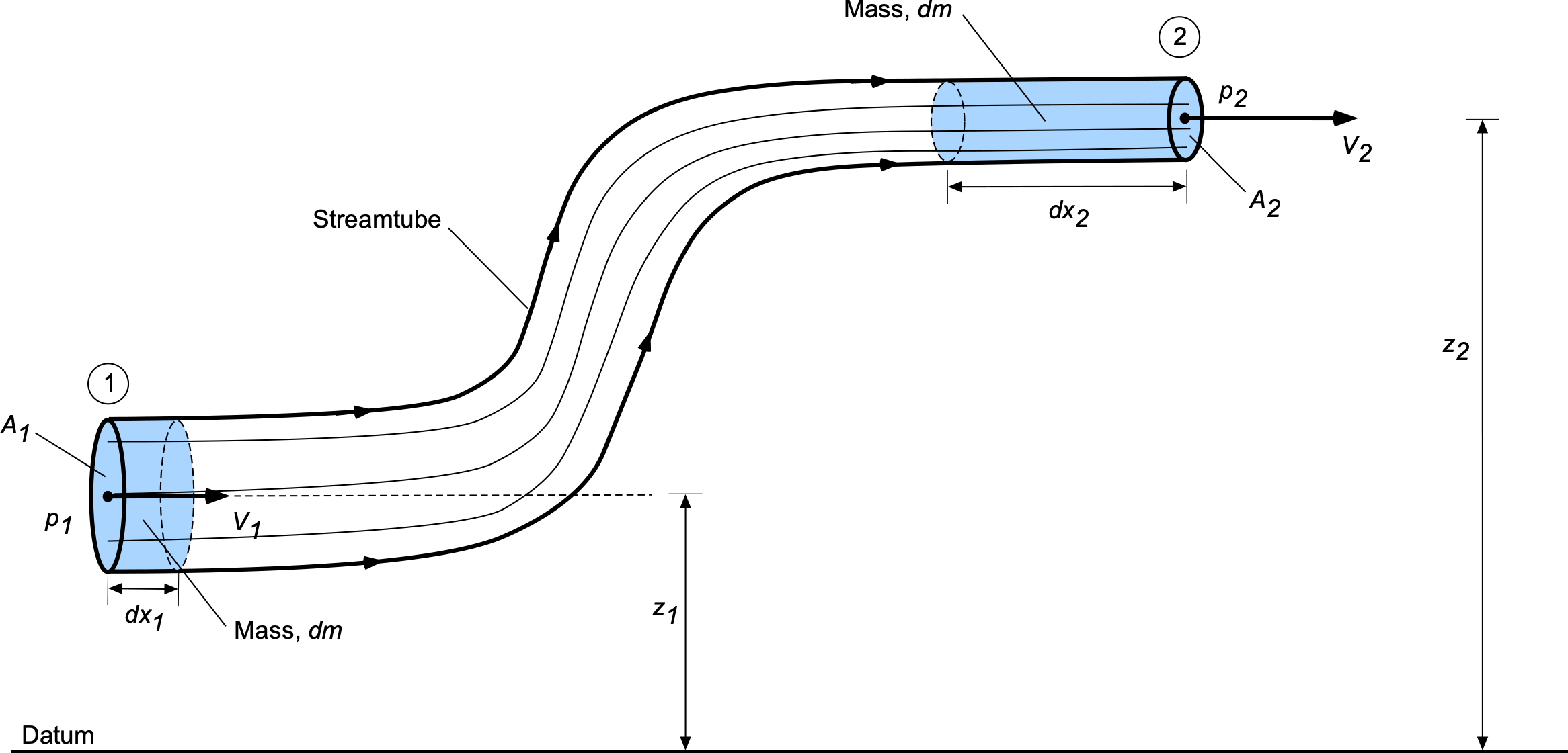
In terms of another physically intuitive derivation of the Bernoulli equation, consider the figure below, which represents a streamtube flow of an ideal fluid that is steady, incompressible, and inviscid. At the inlet to the streamtube, the cross-sectional area is $A_1$ with flow velocity ${V_1}$ and at a height ${z_1}$ from a reference (datum) level. At the outlet, the area is $A_2$ , and the velocity is ${V_2}$ at a height of ${z_2}$ . In a given time, a mass of fluid, $dm$ , can be considered to have moved in the streamtube from the inlet to the outlet.

Streamtube flow model used for the derivation of the Bernoulli equation.

Let $p_1$ be the pressure acting uniformly at the inlet at station 1. Because pressure acts inward, it creates a force that pushes the fluid downstream toward the outlet. The work done by the pressure force here will be

(52) $\begin{equation*} W_1 = \left( p_1 \, A_1 \right) \, dx_1 \end{equation*}$

remembering that work is equal to force times distance. Let $p_2$ be the pressure acting uniformly at the outlet at station 2. In this case, the work done by the pressure force will be

(53) $\begin{equation*} W_2 = -\left( p_2 \, A_2 \right) \, dx_2 \end{equation*}$

Notice that the minus sign here indicates that the pressure force acts upstream in the opposite direction to the fluid flow. In addition, there will be work done under gravity, which will be

(54) $\begin{equation*} W_g = -dm \, g \left( z_2 - z_1 \right) = - \varrho \, d{\cal{V}} \, g \left( z_2 - z_1 \right) \end{equation*}$

where the mass $dm = \varrho \, d{\cal{V}}$ , and the minus sign means that work must be put into the fluid system to increase its potential energy. Therefore, the total external work is

(55) $\begin{equation*} W_1 + W_2 + W_g = p_1 \, A_1 \, dx_1 - p_2 \, A_2 \, dx_2 - \varrho \, d{\cal{V}} \, g \left( z_2 - z_1 \right) \end{equation*}$

The kinetic energy of the flow must now be taken into account. The change in kinetic energy of the fluid as it moves through the streamtube is

(56) $\begin{equation*} \Delta KE = \frac{1}{2} \, dm \, V_2^2 - \frac{1}{2} \, dm \, V_1^2 = \frac{1}{2} \, \varrho \, d {\cal{V}} \, V_2^2 - \frac{1}{2} \, \varrho \, d{\cal{V}} \, V_1^2 \end{equation*}$

The application of the principle of conservation of energy requires that

(57) $\begin{equation*} W_1 + W_2 + W_g = \Delta KE \end{equation*}$

so that

(58) $\begin{equation*} p_1 \, A_1 \, dx_1 - p_2 \, A_2 \, dx_2 - \varrho \, d{\cal{V}} \, g \left( z_2 - z_1 \right) = \frac{1}{2} \, \varrho \, d{\cal{V}} \, V_2^2 - \frac{1}{2} \, \varrho \, d{\cal{V}} \, V_1^2 \end{equation*}$

Notice also that conservation of mass (the continuity equation) requires that

(59) $\begin{equation*} \varrho \, d{\cal{V}} = \varrho \left( A_1 \, dx_1 \right) = \varrho \left( A_2 \, dx_2 \right) \end{equation*}$

or just

(60) $\begin{equation*} A_1 \, dx_1 = \, A_2 \, dx_2 \end{equation*}$

Therefore, inserting the various terms gives

(61) $\begin{equation*} \left( p_1 - p_2 \right) d{\cal{V}} - \varrho \, d{\cal{V}} \, g \, \left( z_2 - z_1 \right) = \frac{1}{2} \, \varrho \, d{\cal{V}} \, \left( V_2^2 - V_1^2 \right) \end{equation*}$

Cancelling out the volume $d{\cal{V}}$ and rearranging this latter equation gives

(62) $\begin{equation*} p_1 + \frac{1}{2} \, \varrho V_1^2 + \varrho \, g \, z_1 = p_2 + \frac{1}{2} \, \varrho V_2^2 + \varrho \, g \, z_2 \end{equation*}$

or

(63) $\begin{equation*} p + \frac{1}{2} \, \varrho \, V^2 + \varrho \, g \, z = \mbox{constant} \end{equation*}$

which, again, is the Bernoulli equation.

Caution: Remember that in the derivation of the Bernoulli equation, the flow has been assumed to be steady and incompressible with negligible frictional or viscous losses (i.e., an ideal fluid), and where no mechanical work is added or subtracted. While the Bernoulli equation is found to have many practical applications, it is essential to remember that it has been derived based on certain prior assumptions. Therefore, its practical use requires considerable justification and caution in actual applications.

Check Your Understanding #2 – Pressure change in a contraction

Air flows at low speed through a pipe with a volume flow rate of 0.135 m ${^3}$ /s. The pipe has an inlet section diameter of 21 cm and an outlet section diameter of 9 cm. A water manometer measures the pressure difference between the inlet and outlet sections. Assuming no frictional losses, determine the differential height $\Delta h$ shown on the manometer. Take the density of air to be 1.21 kg/m ${^3}$ and the density of water to be 1,000 kg/m ${^3}$ . Make any assumptions you feel are justified.

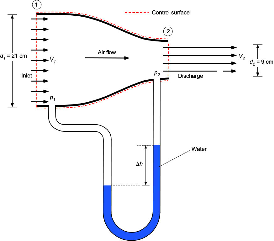
Show solution/hide solution.

Based on the information, assuming a one-dimensional, steady, incompressible, and inviscid flow seems reasonable. The flow rates, velocities, and Mach numbers are low enough that compressibility effects can be neglected. Let the inlet be condition 1 and the outlet condition 2. The continuity equation relates the inlet and outlet conditions, i.e.,

$\overbigdot{m} = \varrho A_1 V_1 = \varrho A_2 V_2 = \mbox{constant}$

Or because the flow is assumed incompressible, then just

${\overbigdot{{\cal{V}}}} = A_1 V_1 = A_2 V_2 = \mbox{constant} = 0.135~\mbox{m${^3}$/s}$

It follows that

$V_1 = \frac{{\overbigdot{{\cal{V}}}} }{A_1}$

and

$V_2 = \frac{{\overbigdot{{\cal{V}}}} }{A_2}$

Calculating the areas gives

$A_1 = \frac{\pi d_1^2}{4} = \frac{\pi \, 0.21^2}{4} = 0.0346~\mbox{m${^{2}}$}$

and

$A_2 = \frac{\pi d_2^2}{4} = \frac{\pi \, 0.09^2}{4} = 0.00636~\mbox{m${^{2}}$}$

Now the velocities can be calculated, i.e.,

$V_1 = \frac{{\overbigdot{{\cal{V}}}} }{A_1} = \frac{0.135}{0.0346} = 3.90~\mbox{m/s}$

and

$V_2 = \frac{{\overbigdot{{\cal{V}}}} }{A_2} = \frac{0.135}{0.00636} = 21.22~\mbox{m/s}$

which are much lower than a Mach number of 0.3, so the assumption of incompressible flow is justified.

The pressure difference between points 1 and 2 is required, which necessitates the use of some form of the energy equation. Using the Bernoulli equation is justified because the given information pertains to an incompressible, frictionless flow. The Bernoulli equation is

$p_1 + \frac{1}{2} \varrho V_1^2 = p_2 + \frac{1}{2} \varrho V_2^2$

so

$p_1 - p_2 = \frac{1}{2} \varrho V_2^2 - \frac{1}{2} \varrho V_1^2 = \frac{1}{2} \varrho \left( V_2^2 - V_1^2 \right)$

Inserting the values for $\varrho$ , ${V_1}$ and ${V_2}$ gives

$p_1 - p_2 = \frac{1}{2} \varrho \left( V_2^2 - V_1^2 \right) = \frac{1}{2} \times 1.21 \left( 21.22^2 - 3.9^2 \right) = 263.25~\mbox{Pa}$

In terms of ${h}$ , which is the differential height on the manometer, then

$p_1 - p_2 = \varrho_{\rm H_2 0} \, g \, h = 263.25~\mbox{Pa}$

so solving for ${h}$ , gives

$h = \frac{p_1 - p_2 }{\varrho_{\rm H_2 0} \, g} = \frac{263.25}{1,000 \times 9.81} = 0.0268~\mbox{m} = 2.68~\mbox{cm}$

Other Forms of the Bernoulli Equation

Other forms of the Bernoulli equation are used. For example, the unintegrated form of the Bernoulli equation is

(64) $\begin{equation*} \int \frac{dp}{\varrho} + \frac{1}{2} V^2 + g z = \mbox{constant} \end{equation*}$

Recall that for an incompressible flow, the first term is

(65) $\begin{equation*} \int \frac{dp}{\varrho} = \frac{p}{\varrho} \end{equation*}$

so the classic Bernoulli equation is recovered, i.e.,

(66) $\begin{equation*} p + \frac{1}{2} \varrho \, V^2 + \varrho g z = \mbox{constant} \end{equation*}$

Isothermal Process

For an isothermal process, $T$ = constant along a streamline in the flow, so from the equation of state, then

(67) $\begin{equation*} \frac{p}{\varrho} = R \, T = \mbox{constant} = C_1 \end{equation*}$

or

(68) $\begin{equation*} \varrho = \frac{p}{C_1 } \end{equation*}$

Therefore,

(69) $\begin{equation*} \int \frac{dp}{\varrho} = C_1 \ln p = \frac{p}{\varrho} \ln p \end{equation*}$

And so the Bernoulli equation for an isothermal flow is

(70) $\begin{equation*} \frac{p}{\varrho} \ln p + \frac{1}{2} V^2 + g z = \mbox{constant} \end{equation*}$

or between two points 1 and 2 (which are on the same streamline), then

(71) $\begin{equation*} \frac{p_1}{\varrho_1} \ln p_1 + \frac{1}{2} V_1^2 + g z_1 = \frac{p_2}{\varrho_2} \ln p_2 + \frac{1}{2} V_2^2 + g z_2 \end{equation*}$

Adiabatic Process

Another case of a compressible flow is an adiabatic process characterized by the relationship

(72) $\begin{equation*} \frac{p}{\varrho^{\gamma}} = C_2 = \mbox{constant} \end{equation*}$

where ${\gamma}$ is the ratio of specific heats. Solving for the density $\varrho$ gives

(73) $\begin{equation*} \varrho = C_2^{(-1/\gamma)} p^{1/\gamma} \end{equation*}$

As previously derived, the unintegrated form of the Bernoulli equation can be written as

(74) $\begin{equation*} \int \frac{dp}{\varrho} + \frac{1}{2} V^2 + g z = \mbox{constant} \end{equation*}$

Substituting for $\varrho$ into the first term gives

(75) $\begin{equation*} \int \frac{dp}{\varrho} = \int C_2^{(1/\gamma)} p^{(-1/\gamma)} dp = \left( \frac{\gamma}{\gamma - 1} \right) \frac{p}{\varrho} \end{equation*}$

Therefore, another form of the Bernoulli equation for the steady, adiabatic, compressible flow of a gas becomes

(76) $\begin{equation*} \left( \frac{\gamma}{\gamma - 1} \right) \frac{p}{\varrho} + \frac{1}{2} V^2 + g z = \mbox{constant} \end{equation*}$

Quasi-Steady Effects

The Bernoulli equation can also be used for certain classes of quasi-steady flows. A quasi-steady flow refers to a flow that is considered to change slowly over time, allowing for some unsteady effects to be accounted for. The assumption is that the unsteady changes occur smoothly and gradually, without large, rapid fluctuations, i.e., in this case, $V = V(t)$ so $\partial V/\partial t \ne 0$ . This situation allows the Bernoulli equation to remain applicable, albeit with a time-dependent term. The so-called “unsteady form” of the equation can be written as

(77) $\begin{equation*} \varrho \dfrac{\partial V}{\partial t} + dp + \dfrac{1}{2} \varrho \, d(V^2) + g dz = 0 \end{equation*}$

where the first term is equivalent to the additional energy involved in accelerating the fluid along the streamline. Such effects usually appear in quasi-steady aerodynamics problems, appearing as “apparent” or added “mass in the forces and moments acting on a body. In true unsteady flow situations, where rapid changes occur (such as in turbulent flows, flows with strong vortices, or flows with large-scale unsteadiness, the Bernoulli equation cannot be applied. A more general form of the energy equation would be needed in such cases.

This quasi-steady form of the Bernoulli equation can be integrated between two points, say point 1 (located at a distance $s_1$ along the length of the streamline) and point 2 (located at a distance $s_1$ ), to give

(78) $\begin{equation*} p_1 + \frac{1}{2} \varrho V_1^2 + \varrho g z_1 = \varrho \int_{s_1}^{s_2} \dfrac{\partial V}{\partial t} ds + p_2 + \frac{1}{2} \varrho V_2^2 + \varrho g z_2 \end{equation*}$

Notice that the “unsteady” pressure term, accounting for acceleration effects in the flow in the direction of $s$ along a streamline, is

(79) $\begin{equation*} \mbox{Unsteady~term} = \varrho \int_{s_1}^{s_2} \dfrac{\partial V}{\partial t} ds \end{equation*}$

In practice, this unsteady term is not easy to calculate except in some simple unsteady flows.

For example, consider an accelerating flow where the velocity at a point changes linearly with time, i.e., constant acceleration, where the velocity is given by

(80) $\begin{equation*} V(t) = V_0 + a \, t \end{equation*}$

where $V_0$ is the initial velocity at $t = 0$ and $a$ is the (constant) acceleration, i.e..

(81) $\begin{equation*} \frac{\partial V}{\partial t} = a \end{equation*}$

To find the unsteady contribution, it must be integrated along a streamline from point $s_1$ to point $s_2$ , i.e.,

(82) $\begin{equation*} \varrho \int_{s_1}^{s_2} \frac{\partial V}{\partial t} \, ds = \varrho \int_{s_1}^{s_2} a \, ds \end{equation*}$

In this case, $a$ is constant, so the integral simplifies to

(83) $\begin{equation*} \varrho \int_{s_1}^{s_2} a \, ds = \varrho a \int_{s_1}^{s_2} ds \end{equation*}$

Notice that

(84) $\begin{equation*} \int_{s_1}^{s_2} ds = s_2 - s_1 \end{equation*}$

so the unsteady term for this flow becomes

(85) $\begin{equation*} \mbox{Unsteady~term} = \varrho \int_{s_1}^{s_2} a \, ds = \varrho \, a (s_2 - s_1) \end{equation*}$

This result is simply part of the flow’s energy balance, accounting for its acceleration.

Energy Equation from the RTE

The Reynolds Transport Theorem (RTE) for the total energy $E$ within a C.V. of volume $\mathcal{V}$ is expressed as

(86) $\begin{equation*} \frac{D}{Dt} \oiiint_{\mathrm{sys}} E \, \varrho \, d\mathcal{V} = \frac{\partial}{\partial t} \oiiint_{\mathcal{V}} E \, \varrho \, d\mathcal{V} + \oiint_{S} E \, \varrho (\vec{V}_{\mathrm{rel}} \bigcdot d\vec{S}) \end{equation*}$

where $E$ is the total energy contained within the C.V. Using the divergence theorem for the surface integral gives

(87) $\begin{equation*} \frac{D}{Dt} \oiiint_{\mathrm{sys}} (E \, \varrho) \, d\mathcal{V} = \oiiint_{\mathcal{V}} \frac{\partial}{\partial t} (E \, \varrho) \, d\mathcal{V} + \oiiint_{\mathcal{V}} (E \, \varrho) (\vec{V} \bigcdot \nabla) \vec{V} \, d\mathcal{V} \end{equation*}$

Furthermore,

(88) $\begin{equation*} \frac{\partial}{\partial t} (E \, \varrho) = \varrho \, \frac{\partial E}{\partial t} + E \frac{\partial \varrho}{\partial t} \end{equation*}$

For an incompressible flow, $\dfrac{\partial \varrho}{\partial t} = 0$ , so

(89) $\begin{equation*} \frac{\partial}{\partial t} (E \, \varrho) = \varrho \, \frac{\partial E}{\partial t} \end{equation*}$

Therefore, the energy equation in differential form is

(90) $\begin{equation*} \varrho \frac{D e}{Dt} = \varrho \, \frac{\partial e}{\partial t} + \varrho (\vec{V} \bigcdot \nabla) e = \frac{\partial}{\partial t} (\varrho \, e) + (\varrho \, e) (\vec{V} \bigcdot \nabla) \vec{V} \end{equation*}$

where $\dfrac{D e}{Dt}$ is the substantial derivative of specific internal energy ${e}$ , i.e.,

(91) $\begin{equation*} \frac{D e}{Dt} = \frac{\partial e}{\partial t} + (\vec{V} \bigcdot \nabla) e \end{equation*}$

This equation represents energy conservation for a fluid, accounting for changes in internal energy ${e}$ from both convective transport and local changes in time and space.

From the energy equation, then

(92) $\begin{equation*} \varrho \frac{D e}{Dt} = \frac{\partial}{\partial t} (\varrho \, e) + (\varrho \, e) (\vec{V} \bigcdot \nabla) \vec{V} \end{equation*}$

Assuming steady, inviscid flow where $\dfrac{\partial}{\partial t} = 0$ and neglecting viscosity effects ( $\mu \, \nabla^2 \vec{V} = 0$ ), the energy equation simplifies to

(93) $\begin{equation*} { \varrho \frac{D e}{Dt} = 0 } \end{equation*}$

This result implies that the specific internal energy ${e}$ remains constant along a streamline in inviscid flow. Therefore, integrating along a streamline gives

(94) $\begin{equation*} \varrho \left( \frac{V^2}{2} + e + g \, z \right) = \text{constant} \end{equation*}$

Assuming constant density, i.e., $\varrho$ = constant, then the Bernoulli equation can be expressed in terms of pressure $p = \varrho \, e$ as

(95) $\begin{equation*} p + \frac{1}{2} \varrho \, V^2 + \varrho g \, z = \text{constant} \end{equation*}$

Once again, this is the Bernoulli equation for steady, inviscid, and incompressible flow.

Summary & Closure

Applying the principle of energy conservation to fluid flow results in a rather formidable-looking equation in its more general form. The energy equation is derived from thermodynamic principles, specifically the first law of thermodynamics, and utilizes the concepts of heat, work, and power. The types of energy involved in most fluid problems are internal, potential, and kinetic energy. The energy equation is a power equation based on its units, i.e., the rate of doing work. When thermodynamic principles are involved in fluid flow problems, the equation of state is also helpful in establishing the relationships between the known and unknown quantities.

The most common application of the energy equation is to so-called single-stream systems, in which a certain amount of fluid energy comes into a system where work is added or extracted. Then, the energy can exit the system in another form. Further simplifying the energy equation to incompressible, inviscid flows without energy addition yields the Bernoulli equation, which can be successfully applied to many practical problems to relate pressures and flow velocities. The Bernoulli equation is also a statement of energy conservation, i.e., fluid exchanges its specific kinetic energy for static or potential pressure. Nevertheless, the Bernoulli equation must be used carefully and consistently applied within the assumptions and limitations of its derivation.

5-Question Self-Assessment Quickquiz

For Further Thought or Discussion

The energy equation is often referred to as a redundant equation for analyzing incompressible, inviscid flows. Why?
What are the three main assumptions used in deriving the Bernoulli equation?
The flow through the turbine blades of a jet engine can be modeled using the incompressible form of the Bernoulli equation. True or false? Explain.
In conjunction with the conservation of mass and momentum, the Bernoulli equation can be used to analyze the flow through a propeller operating at low flow speeds. Could you explain how to do that?

Additional Online Resources

To learn more about the energy equation, as well as the Bernoulli equation and its uses, check out some of these online resources:

A good video on the first law of thermodynamics and internal energy.
Video sequence from Dr. Biddle’s YouTube channel on fluid mechanics.
A video lecture describing the derivation of the energy equation for a fluid.
Video on conservation of energy in control volume form.
This is an excellent video on better understanding the Bernoulli equation.
The use of graphics in this video reinforces the meaning of the Bernoulli equation.
Another good video describing the applications of the Bernoulli equation.

License

Icon for the Creative Commons Attribution-NonCommercial-NoDerivatives 4.0 International License

Introduction to Aerospace Flight Vehicles Copyright © 2022–2025 by J. Gordon Leishman is licensed under a Creative Commons Attribution-NonCommercial-NoDerivatives 4.0 International License, except where otherwise noted.

Digital Object Identifier (DOI)

https://doi.org/https://doi.org/10.15394/eaglepub.2022.1066.n18