Equations of Fluid Motion

J. Gordon Leishman

18 Equations of Fluid Motion

Introduction

Solving problems in fluid dynamics and aerodynamics requires that appropriate mathematical models of the flow field be set up correctly. The derivation of the mathematical equations that describe fluid dynamics and aerodynamic flows is relatively straightforward because it is a systematic process that has become well-established in engineering practice. However, all practical problems will inevitably require some assumptions and approximations to the equations to obtain solutions, a common (and valid) assumption being that air behaves as an ideal gas. Other assumptions include two-dimensional, steady, inviscid, and incompressible flow. Part of the skill in solving problems in fluid dynamics and aerodynamics problems is understanding what reference frames and sets or subsets of equations are needed.

Learning Objectives

Understand how the conservation principles are applied to solve fluid dynamic and aerodynamic problems.
Appreciate the various types of flow models that can be used to solve fluid problems.
Understand the concepts of mass flux and mass flow.
Know how to set up a finite control volume model of a fluid flow.
Appreciate how the Reynolds Transport Equation (RTE) is derived and its uses.

Setting up Flow Models

Setting up flow models in fluid dynamics and aerodynamics involves creating mathematical representations of fluid behavior to analyze and predict fluid flow patterns such as streamlines, pressures, velocities, and other related parameters. These flow models are a foundation for understanding and solving real-world engineering problems in aerospace engineering and other disciplines.

Problem Definition: The first step is clearly defining the problem to be solved, which inevitably raises questions. Try to identify the type of fluid flow – is it incompressible or compressible, steady or unsteady, laminar or turbulent? What is the geometry of the fluid system, the boundary conditions, and the desired outcomes, e.g., flow rates, flow, velocities, pressure distributions, etc.?
Governing Equations: Select the appropriate governing equations likely to describe fluid flow behavior. These typically include the continuity, momentum, and energy equations. If justified, additional equations, such as the equation of state, may be applied to specific problems.
Assumptions and Simplifications: Make any assumptions and simplifications that might reduce the complexity of the equations while ensuring that they remain relevant to the problem. Typical assumptions include neglecting specific forces (e.g., viscosity) or considering steady-state conditions.
Boundary Conditions: Specify appropriate boundary conditions at the system’s boundaries. These conditions can include prescribed velocities, pressures, temperature, and any other relevant parameters. Boundary conditions will be crucial in determining fluid behavior within and out of the system.
Post-Processing: Analyze the results obtained from the flow model. If needed, generate plots, tables, and other visualizations to gain insights into the flow behavior and validate the model against experimental measurements.

Conservation equations

The three fundamental conservation principles of mechanics must be applied to solve the fluid dynamic or aerodynamic problem, namely:

Conservation of mass, i.e., mass is neither created nor destroyed.
Conservation of momentum, i.e., a force acting on a mass equals its time rate of change of momentum.
Conservation of energy, i.e., energy is neither created nor destroyed and can only be converted from one form into another.

The resulting mathematical equations should then describe the fluid dynamic or aerodynamic behavior of the flow of interest, at least within the bounds of the stated assumptions and approximations. The solution to these equations can proceed analytically, numerically, or both, hopefully giving an engineer the desired results.

Flow Models

There are two basic approaches used in fluid dynamics and aerodynamics:

An integral or finite control volume approach in which the equations are developed as they apply to a finite control volume surrounding the problem.
The differential or infinitesimal fluid element approach in which the relevant equations apply at every flow point.

In both approaches, the control volume or the fluid element may be fixed in space, and the flow moves through it, or it may move with the flow, containing the same group of fluid molecules. The former approach (i.e., fixed in space) is called an Eulerian model, as shown in the figure below, and the latter (i.e., moves with the flow) is called a Lagrangian model. Each of these modeling approaches has certain advantages and disadvantages when applied to solving specific problems in aerodynamics. In most cases, there will be a preferred approach for each problem.

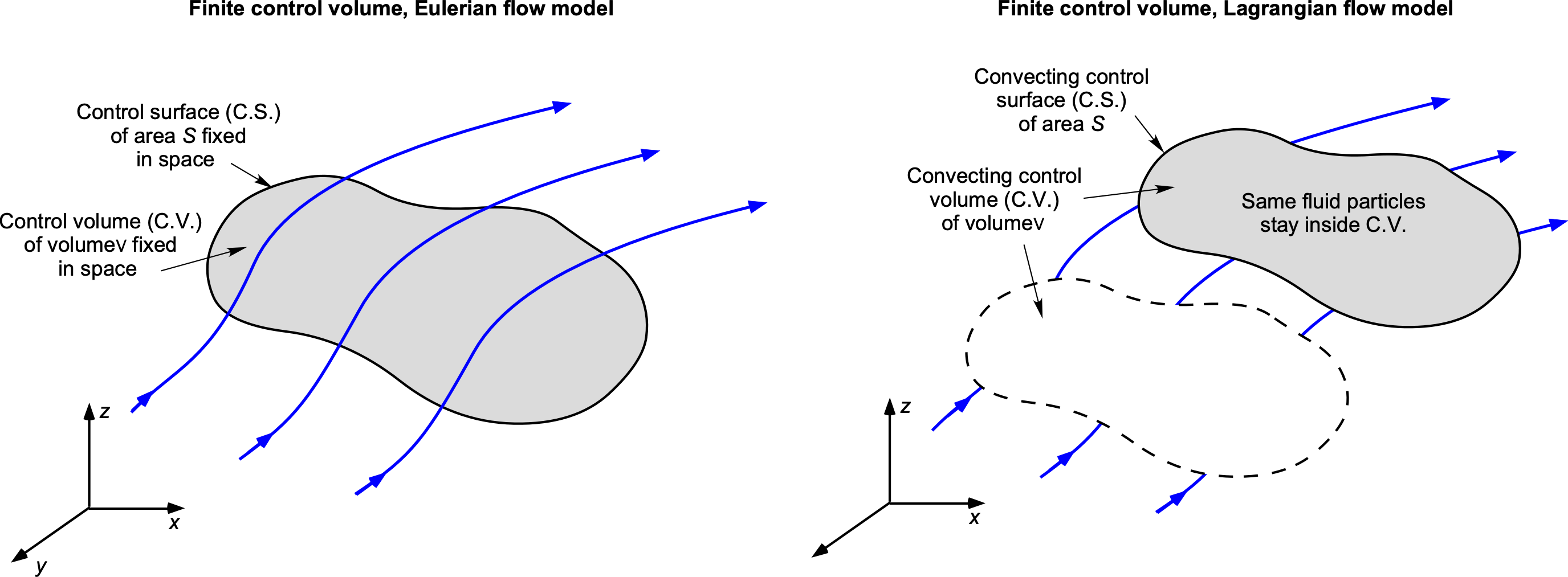
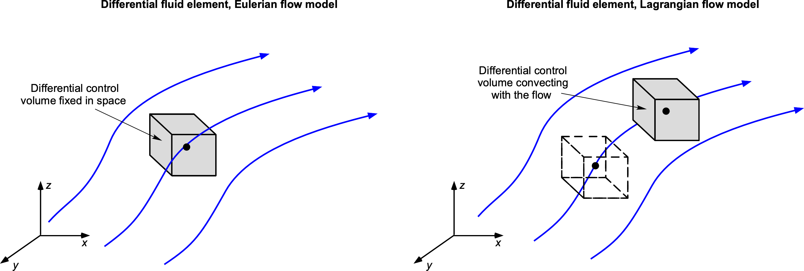
Control volume approach to solve aerodynamic problems. An Eulerian representation is a fixed control volume in space with the fluid elements flowing in and out of the control volume. A convecting control volume carrying the same fluid elements is called a Lagrangian representation.

For example, on the one hand, an integral approach could be used to find total effects, such as the forces on a body in the flow, but without necessarily solving for all of the point properties in the flow. Knowing what the fluid is doing at the flow at every point may not be necessary, and an integrated approach may be more appropriate. On the other hand, the differential approach, as shown in the figure below, would be needed if the local distributions of flow velocity and pressure at points in the flow and over the surface of a body were the desired outcome.

Differential fluid element approach to solving aerodynamic problems. A fixed elemental volume in space with the fluid flowing in and out is called an Eulerian representation, the convecting volume being a Lagrangian representation.

Likewise, a Lagrangian approach might be adopted over an Eulerian approach because it makes the problem description more manageable in modeling the physical problem and/or from a mathematical description and/or solution methodology. Part of the skills needed in fluid dynamics and aerodynamics problem solving (and engineering problem solving, in general) is to decide which type of basic model to apply to specific problems. Sometimes, such decisions may not be obvious even for an experienced engineer, and different approaches may need to be tried tentatively before deciding.

For example, it may be desired to predict the velocity and pressure distribution over the surface of an airfoil or wing, as shown in the figure below. The question is then: What basic form of the aerodynamic model should be used? In this case, the answer is a differential model in that point properties such as flow velocity, streamlines, and pressures could be determined. Integral forms of the equations would be appropriate only when the overall or integrated aerodynamic effects are needed. The total lift on the wing is an integral quantity because it arises from the effects of the pressure distribution when it is resolved and integrated over the wing’s surface.

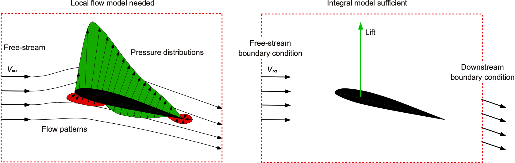
Point flow properties require a local flow model, but integrated quantities can be determined from a control volume approach.

In practice, the integral approach is usually easier to learn and work with, at least from a mathematics and/or numerical perspective. The differential form of the equations would be appropriate when the distributive quantities, such as when the velocity and pressure distributions over the wing’s surface, are needed, which are usually more computationally expensive. Again, the relative cost of obtaining a solution for the flow properties may need to be factored into the final choice of the model.

Finite Control Volume Approach

To introduce the conservation laws of fluid dynamics, it is convenient to focus on finite control volume or integral models, which are helpful in that they can be used to relate the global properties of the fluid. The concern is with the fluid properties coming into the control volume versus what changes to the properties come out. However, in many other practical problems, fluid properties at a point in the flow may be required, so using the differential (fluid element) model and applying this modeling approach to problem-solving is usually necessary.

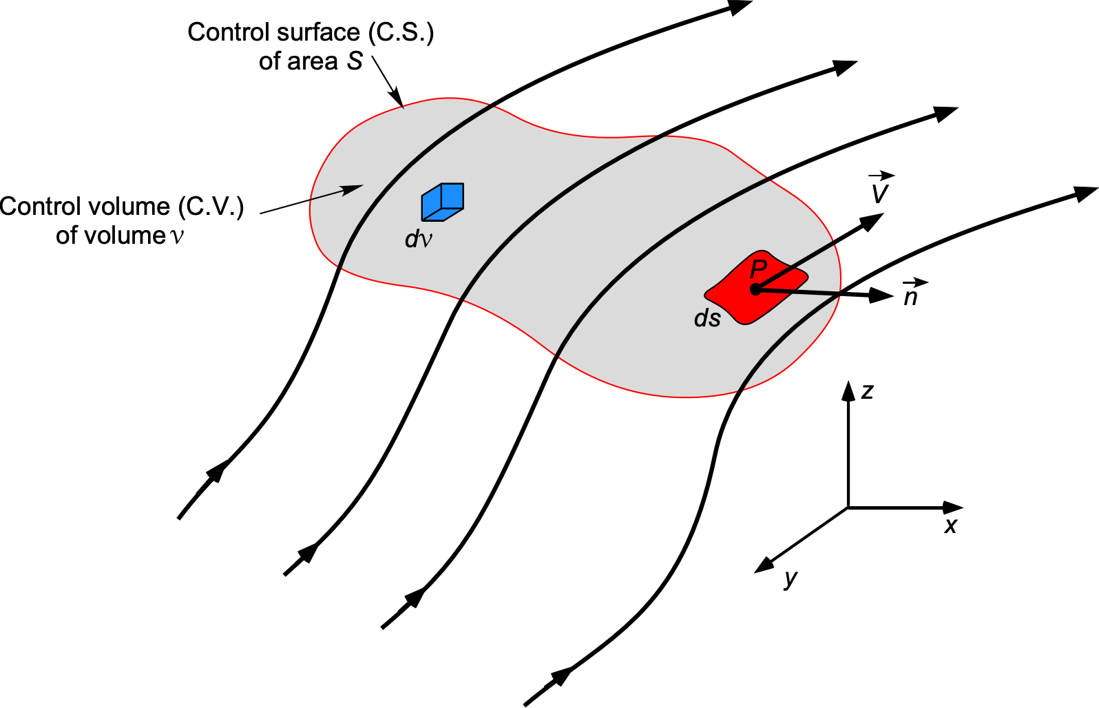
In the finite control volume approach, a closed surface is drawn to contain a specific flow volume, as shown in the figure below. The symbol $S$ defines the area of the closed surface that bounds the control volume containing a fluid of volume $\cal{V}$ . The control volume is abbreviated to “C.V.” (denoted by ${\cal{V}}$ in the mathematics) and the control surface to “C.S.” denoted by $S$ in the mathematics). This control surface (and control volume) must be large enough to contain the domain of the entire problem. In some cases, the needed control volumes may be required to cover only part of the domain if certain flow conditions are known or defined elsewhere, which is common in practice. One of the problem-solving techniques that engineers must develop is to determine the most suitable control surface/volume so that the governing equations can be applied and the correct solutions for the flow properties can be obtained.

A finite control volume, fixed in space, with the fluid flowing in and out across a control surface.

All fluid properties can and must be allowed to vary with spatial location (i.e., with respect to $x$ , $y$ , and $z$ ) and in time $t$ so that

(1) $\begin{eqnarray*} \varrho & = & \varrho ( x, y, z, t ) \\[6pt] \vec{V} & = & \vec{V} (x, y, z, t) \end{eqnarray*}$

As previously described, $dS$ is a small elemental area of the control surface, and the vector $\vec{n}$ is the unit normal vector. Because the product $\vec{n} \, dS$ appears in the resulting equations for the flow, the unit normal vector area is defined as $d\vec{S} = \vec{n} \, dS$ . Remember that by convention $\vec{n}$ , and so also $d\vec{S}$ , always points outward from the control volume perpendicular to the control surface. For example, if the surface is oriented perpendicular to the flow in the $x$ direction (i.e., in the $y$ – $z$ plane), then $\vec{n} = (1, 0, 0)$ and if the surface is oriented perpendicular to the $z$ direction (i.e., in the $x$ – $y$ plane) then $\vec{n} = (0, 0, 1)$ .

Notice: Be cautious not to confuse the symbol for velocity (a vector $\vec{V}$ or $\bf V$ with the symbol for volume $\cal{V}$ or a “curly V.” Sometimes the symbol $\volume$ is used rather than $\cal{V}$ , but the meaning (volume) is the same.

Mass Flow and Mass Flux

Before deriving the fundamental equations used in fluid dynamics or aerodynamics, one must examine a concept vital to all these equations: mass flow. Consider a small, fully permeable surface of differential area $dS$ that is oriented at some angle in a flow, as shown in the figure below.

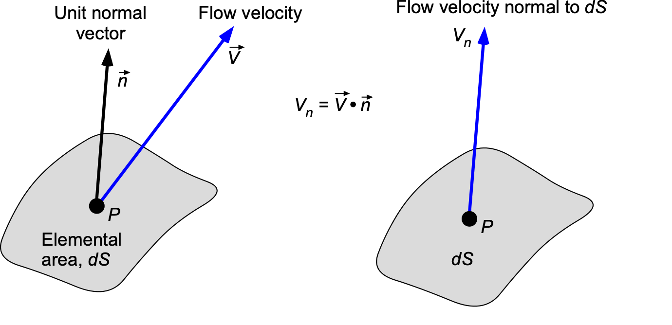The mass flow through an area $dS$ requires the calculation of the flow velocity normal to the surface.

Let the area $dS$ be small enough so that the velocity of the flow is constant across it, i.e., in the spirit of the differential calculus. Then, consider the orientation of the small surface to be defined in terms of a unit normal vector $\vec{n}$ . The normal unit vector $\vec{n}$ establishes the orientation of the surface where $\vec{n}$ is perpendicular to the curvature of the surface and points away from the surface. The mass flow $d\overbigdot{m}$ through the surface $dS$ per unit time (the mass flow rate) will be given by

(2) $\begin{equation*} d\overbigdot{m} = \varrho V_{n} dS = \varrho ( \vec{V} \bigcdot \vec{n} ) dS \end{equation*}$

where $V_n$ is the magnitude of the resultant flow velocity normal to the surface. Remember that if $\vec{V}$ is the velocity of the flow through the surface, then the component of the resultant flow velocity normal (perpendicular) to the surface is given by the dot-product

(3) $\begin{equation*} | V_n | = \vec{V} \bigcdot \vec{n} \end{equation*}$

The concept is better visualized in two dimensions, as shown in the figure below. Notice that the unit normal vector area is defined as $d\vec{S} = \vec{n} dS$ , so that

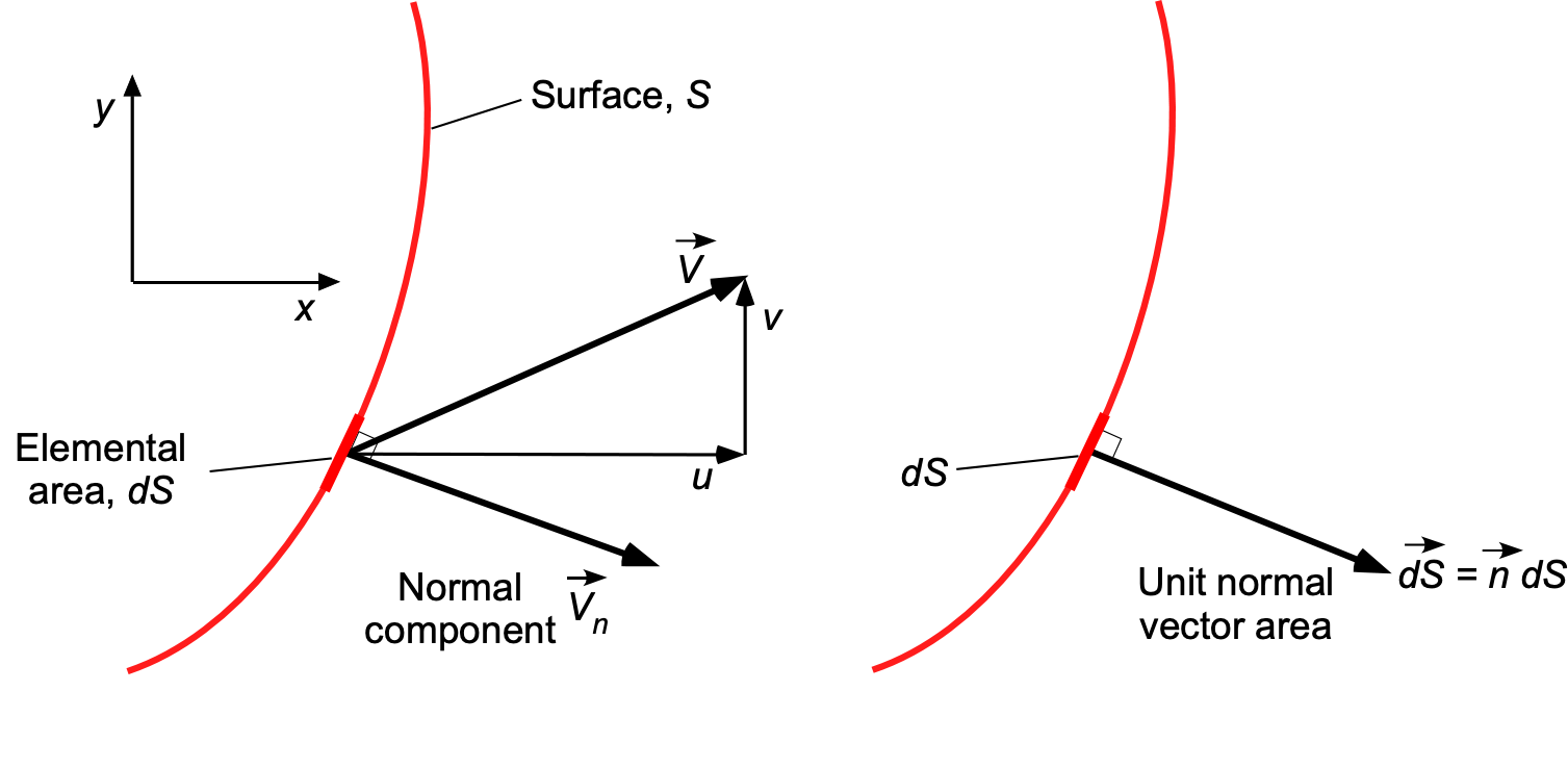
(4) $\begin{equation*} d\overbigdot{m} = \varrho ( \vec{V} \bigcdot \vec{n} ) dS = \varrho ( \vec{V} \bigcdot d\vec{S} ) \end{equation*}$

The velocity component acting normal to a surface is represented in two dimensions. The standard method of representing the normal vector in the fluid equations uses the unit normal vector area.

In this two-dimensional case, then

(5) $\begin{equation*} \vec{V} = u \, \vec{i} + v \, \vec{j} \end{equation*}$

and

(6) $\begin{equation*} \vec{n} = n_x \, \vec{i} + n_y \, \vec{j} \end{equation*}$

so

(7) $\begin{equation*} | V_n | = \left( u \vec{i} + v \vec{j} \right) \bigcdot \left( n_x \vec{i} + n_y \vec{j} \right) = u \, n_x + v \, n_y \end{equation*}$

In general, the total mass flow rate, $\overbigdot{m} =$ , over a surface $S$ , is given by

(8) $\begin{equation*} \overbigdot{m} = \int_S \varrho ( \vec{V} \bigcdot \vec{n} ) dS = \int_S \varrho ( \vec{V} \bigcdot d\vec{S} ) \end{equation*}$

Mass flow rate has dimensions ( $\rm M L^{-3}$ ) ( $\rm L T^{-1}$ ) ( $\rm L^2$ ) = $\rm M T^{-1}$ and so the units will be in kg s $^{-1}$ in SI units or slugs s $^{-1}$ in USC units.

The mass flux is defined as

(9) $\begin{equation*} \frac{d\overbigdot{m}}{dS} = \varrho V_{n} = \varrho ( \vec{V} \bigcdot \vec{n} ) \end{equation*}$

which has has dimensions ( $\rm M L^{-3}$ ) ( $\rm L T^{-1}$ ) = $\rm M T ^{-1} L^{-2}$ and so units of kg s $^{-1}$ m $^{-2}$ or slugs s $^{-1}$ ft $^{-2}$ . The mass flux terms like $\varrho u,\varrho v,\varrho w$ , etc., frequently occur in fluid dynamic problem solving, so the meaning of these terms should be understood. The concepts of mass flux and unit normal vector area are also used in deriving the governing equations for fluid dynamics and aerodynamic flows.

Momentum & Energy Flow Rates

The corresponding momentum and energy flow rates can also be derived. The momentum flow $d \overline{m} /dt$ through the surface $dS$ per unit time (the momentum flow rate) will be

(10) $\begin{equation*} \frac{ d \overline{m}}{dt} = \varrho \, ( \vec{V} \bigcdot d\vec{S}) \, \vec{V} \end{equation*}$

Therefore, the total momentum flow rate, $\overbigdot{\overline{m}}$ , over a surface, $S$ , is given by

(11) $\begin{equation*} \overbigdot{\overline{m}} = \int_S \varrho \, ( \vec{V} \bigcdot d\vec{S} ) \, \vec{V} \end{equation*}$

which is a vector equation with three components in Cartesian space. Momentum flow rate has dimensions of ( $\rm M L^{-3}$ ) ( $\rm L T^{-1}$ ) $^2$ ( $\rm L^2$ ) = $\rm M L T^{-2}$ and so its units will be kg m s $^{-2}$ in SI units or slugs ft s $^{-2}$ in USC units.

The kinetic energy flow $d(\overbigdot{KE})$ through the surface $dS$ per unit time (the kinetic energy flow rate) will be

(12) $\begin{equation*} d(\overbigdot{KE}) = \frac{1}{2} \varrho \, ( \vec{V} \bigcdot d\vec{S} ) \, \vec{V}^2 \end{equation*}$

Therefore, the total flow rate of kinetic energy, $\overbigdot{m} \vec{V}$ , over a surface $S$ , is given by

(13) $\begin{equation*} \overbigdot{KE} = \frac{1}{2} \int_S \varrho \, ( \vec{V} \bigcdot d\vec{S} ) \, \vec{V}^2 \end{equation*}$

Kinetic energy flow rate has dimensions ( $\rm M L^{-2}$ ) ( $\rm L T^{-1}$ ) ( $L^2$ ) ( $\rm L T^{-1})^2 = M L^{2} T^{-3}$ and so the units will be those of power, i.e., so kg m s $^{-3}$ or J s $^{-1}$ or Watts (W) in SI units or lb-ft s $^{-1}$ in USC units.

Extensive & Intensive Properties

The conservation laws involve the rates of change of extensive properties, which are proportional to the mass of fluid contained within the control volume. The three extensive properties, which are all transportable by the flow, are those previously considered, i.e., mass, momentum, and energy, so that

(14) $\begin{eqnarray*} \mbox{Mass:} \ m & = m (1) \\[6pt] \mbox{Momentum:} \ m \vec{V} & = m (\vec{V}) \\[6pt] \mbox{Energy:} \ E & = m (e) \end{eqnarray*}$

where $e$ is called the specific energy.

The extensive properties, i.e., $m$ , $m \vec{V}$ , and $E$ , which depend on the extent of the system, are designated by the general symbol $B$ . The corresponding intensive properties, denoted by $1$ , $\vec{V}$ , and $e$ , are generally expressed as “per unit mass” and designated by the symbol $\beta$ . The extensive and intensive properties are related by

(15) $\begin{equation*} \beta = \frac{B}{m} \end{equation*}$

Because the density of a fluid can change from point to point, it is always best to express the governing equations as per unit mass. The intensive properties do not depend on the mass or extent of the system.

Reynolds Transport Theorem

The Reynolds Transport Theorem (RTT) or Reynolds Transport Equation (RTE) allows one to derive the governing equations of fluid motion and convert from Lagrangian to Eulerian reference systems, a valuable problem-solving tool. Because the RTE connects governing equations in separate reference systems, it is sometimes called a link equation.

The approach to its derivation proceeds by defining a control system (sys) of fluid and a control volume (C.V.), as previously discussed, as shown in the figure below. The system is a collection of fluid molecules of density $\varrho(x, y, z, t)$ that sweeps into and out of the C.V. At some time, $t - \delta t$ , the system moves toward the C.V. At the time, $t$ , the system, and the C.V. are coincident, i.e., they occupy the same space. At some later time, $t + \delta t$ , the fluid system moves out of the C.V. Therefore, this means that some of the fluid moves out of the C.V., some of the fluid remains inside the C.V., and some fluid comes into the C.V. to replace the fluid and properties that has moved out. In the derivation of the RTT, it becomes a matter of tracking and formally quantifying where all of this fluid goes.

Flow model used to derive the Reynolds Transport Theorem (RTT).

Consider a small element of volume $d {\cal{V}}$ as shown in the figure below. The density of the flow is $\varrho = \varrho ( x, y, z, t )$ and the flow velocity relative to the C.V. is $\vec{V} = \vec{V} (x, y, z, t)$ . If $\beta$ is one of the transportable intensive quantities, i.e., mass, momentum, and energy, then the corresponding extensive properties inside the small value are

(16) $\begin{equation*} dB_{\rm sys} = \beta \, \varrho \, d {\cal{V}} \end{equation*}$

The net value of the extensive property can be obtained by integrating over the entire control volume.

Integrating over the entire system volume then gives

(17) $\begin{equation*} B_{\rm sys} = \oiiint_{\rm sys} \beta \, \varrho \, d {\cal{V}} \end{equation*}$

Similarly, integrating over the C.V. gives

(18) $\begin{equation*} B_{{\cal{V}}} = \oiiint_{{\cal{V}}} \beta \, \varrho \, d {\cal{V}} \end{equation*}$

Notice that at time $t$ , then

(19) $\begin{equation*} B_{\rm sys}(t) = B_{{\cal{V}}}(t) \end{equation*}$

but at time $t +\delta t$ , then

(20) $\begin{equation*} B_{S}(t + \delta t) \ne B_{{\cal{V}}}(t + \delta t) \end{equation*}$

Let $B_{\rm in}$ be an extensive property of the fluid coming into the C.V. and $B_{\rm out}$ be the same extensive property of fluid coming out of the C.V., as shown in the figure below. It will be apparent then that

(21) $\begin{equation*} B_{{\cal{V}}}(t + \delta t) = B_{\rm sys}(t + \delta t) - B_{\rm out}(t + \delta t) + B_{\rm in}(t + \delta t) \end{equation*}$

After rearrangement then

(22) $\begin{equation*} B_{{\cal{V}}}(t + \delta t) - B_{\rm sys}(t) = B_{S}(t + \delta t) - B_{\rm sys}(t ) - B_{\rm out}(t + \delta t) + B_{\rm in}(t + \delta t) \end{equation*}$

Principle of the inward and outward flow of the extensive property from the control volume.

Recall that $B_{\rm sys}(t) = B_{{\cal{V}}}(t)$ , so

(23) $\begin{equation*} B_{{\cal{V}}}(t + \delta t) - B_{{\cal{V}}}(t) = B_{\rm sys}(t + \delta t) - B_{\rm sys}(t ) + B_{\rm out}(t + \delta t) + B_{\rm in}(t + \delta t) \end{equation*}$

and dividing by $\delta t$ gives

(24) $\begin{equation*} \frac{B_{{\cal{V}}}(t + \delta t) - B_{{\cal{V}}}(t)}{\delta t} = \frac{ B_{\rm sys}(t + \delta t) - B_{\rm sys}(t )}{\delta t} - \frac{B_{\rm out}(t + \delta t)}{\delta t} + \frac{B_{\rm in}(t + \delta t)}{\delta t} \end{equation*}$

which begins to look like a differential equation. Notice that the last two terms in Eq. 24 can also be expressed as

(25) $\begin{equation*} \frac{B_{\rm out}(t + \delta t)}{\delta t} = \frac{B_{\rm out}(t + \delta t) - B_{\rm out}(t)}{\delta t} \end{equation*}$

because $B_{\rm out}(t) = 0$ , and

(26) $\begin{equation*} \frac{B_{\rm in}(t + \delta t)}{\delta t} = \frac{B_{\rm in}(t + \delta t) - B_{\rm in}(t)}{\delta t} \end{equation*}$

because $B_{\rm in}(t) = 0$ .

In the limit as $\delta t \rightarrow dt$ then Eq. 24 becomes

(27) $\begin{equation*} \frac{d}{dt} \left( B_{{\cal{V}}} \right) = \frac{d}{dt} \left( B_{\rm sys} \right) - \frac{d}{dt} \left( B_{\rm out} \right) + \frac{d}{dt} \left( B_{\rm in} \right) \end{equation*}$

or by rearrangement, then

(28) $\begin{equation*} \frac{d}{dt} \left( B_{\rm sys} \right) = \frac{d}{dt} \left( B_{{\cal{V}}} \right) + \frac{d}{dt} \left( B_{\rm out} - B_{\rm in} \right) \end{equation*}$

which is a differential equation. Substituting for $B_{\rm sys}$ from Eq. 17 and $B_{{\cal{V}}}$ from Eq. 18 gives

(29) $\begin{equation*} \\[4pt] \frac{d}{dt} \oiiint_{\rm sys} \beta \, \varrho \, d {\cal{V}} = \frac{d}{dt} \oiiint_{{\cal{V}}} \beta \, \varrho \, d {\cal{V}} + \frac{d}{dt} \left( B_{\rm out} - B_{\rm in} \right) \end{equation*}$

This previous equation helps connect fluid properties from a Lagrangian flow perspective, i.e., the fluid system that is moving with the flow, to the properties in an Eulerian perspective, i.e., the properties in a C.V. fixed in the flow. However, the C.V. does not have to be of fixed size, so its shape and size could change over time.

The last term in Eq. 29 now requires further attention. It is apparent from the adopted flow model that some fluid comes into and out of the C.V., so there must be some net relative velocity of the fluid out of the C.V. Consider a small area of the control surface, C.S., of area $dS$ , its orientation specified by the unit normal vector $\vec{n}$ , as shown in the figure below. The relative velocity of the flow out of the C.V. over the C.S. will be

(30) $\begin{equation*} \vec{V}_{\rm rel} = \vec{V}_{\rm sys} - \vec{V}_{\rm C.V.} = \vec{V}_{\rm sys} - \vec{V}_{{\cal{V}}} \end{equation*}$

While many problems in fluid dynamics and aerodynamics will have a fixed C.V. in space and time, it is still possible that the C.V. can be deforming, hence the existence of a component $\vec{V}_{{\cal{V}}}$ .

Calculating the net mass flux requires the consideration of the relative flow velocities of the C.V. and the system.

The volumetric flow rate $dQ$ over the surface will be the product of the component of flow velocity $V_{\rm rel}$ that is normal the area $dS$ over which it flows, i.e.,

(31) $\begin{equation*} dQ = \left( \vec{V}_{\rm rel} \bigcdot \vec{n} \right) \, dS = \vec{V}_{\rm rel} \bigcdot d\vec{S} \end{equation*}$

The dot or scalar product gives the component of the volume flow that is normal to the surface. The corresponding mass flow rate is then found by multiplying by the local flow density, i.e.,

(32) $\begin{equation*} d\overbigdot{m} = \varrho (\vec{V}_{\rm rel} \bigcdot d\vec{S} ) \end{equation*}$

In terms of intensive properties, then

(33) $\begin{equation*} d\overbigdot{B}_{\rm net} = \beta \, \varrho ( \vec{V}_{\rm rel} \bigcdot d\vec{S}) \end{equation*}$

Integrating over the control surface gives

(34) $\begin{equation*} \overbigdot{B}_{\rm net} = \oiint_{S} d\overbigdot{B}_{\rm net} \end{equation*}$

Therefore,

(35) $\begin{equation*} \frac{d}{dt} \left( B_{\rm out} - B_{\rm in} \right) = \frac{d}{dt} \left( B_{\rm net} \right) = \overbigdot{B}_{\rm net} = \oiint_{S} d\overbigdot{B}_{\rm net} = \oiint_{S} \beta \, \varrho ( \vec{V}_{\rm rel} \bigcdot d\vec{S} ) \end{equation*}$

Finally, after updating the terms and organizing everything, then

(36) $\begin{equation*} \frac{d}{dt} \oiiint_{\rm sys} \beta \, \varrho \, d {\cal{V}} = \frac{d}{dt} \oiiint_{{\cal{V}}} \beta \, \varrho \, d {\cal{V}} + \iint_{S} \beta \, \varrho ( \vec{V}_{\rm rel} \bigcdot d\vec{S} ) \end{equation*}$

which is called the Reynolds Transport Equation (RTE). In other words, this equation states that the time rate of change of an extensive flow property, $B$ , in the system is equal to the time rate of change of $B$ in the control volume plus the rate at which $B$ is leaving through the control surface, i.e.,

(37) $\begin{equation*} \underbrace{\frac{D}{Dt} \oiiint_{\mathrm{sys}} \beta \, \varrho \, d\mathcal{V}}_{\begin{tabular}{c} \scriptsize Time rate of \\[-3pt] \scriptsize change of $B$ \\[-3pt] \scriptsize inside the system.\end{tabular}} = \underbrace{\frac{\partial}{\partial t} \oiiint_{\mathcal{V}} \beta \, \varrho \, d\mathcal{V}}_{\begin{tabular}{c} \scriptsize Time rate \\[-3pt] \scriptsize of change of $B$ inside\\[-3pt] \scriptsize the control volume.\end{tabular}} + \underbrace{\oiint_{S} \beta \, \varrho ( \vec{V}_{\mathrm{rel}} \bigcdot d\vec{S}) }_{\begin{tabular}{c} \scriptsize Rate at which $B$ is \\ [-3pt]\scriptsize leaving through the \\[-3pt] \scriptsize control surface.\end{tabular} } \end{equation*}$

Traditionally, the lowercase “ $d$ ” on the left-hand side of Eq. 36 is replaced by “ $D$ ,” implying that it is the time rate of change of properties in a “system.” This derivative is often called the material or substantive derivative. Notice that the first term on the right-hand side of Eq. 36 is now replaced by the partial derivative because, generally, $\beta = \beta (x, y, z, t)$ .

Remember that the RTE allows one to relate flows in Lagrangian and Eulerian reference systems. It also helps to derive the conservation laws of fluid dynamics and aerodynamics for mass, momentum, and energy. For these reasons, it is called a “link” equation because it connects the governing equations in both reference systems.

What are the units of the Reynolds Transport Equation?

The Reynolds Transport Equation (RTE) relates to the time rate of change of an extensive flow property, $B$ . The three extensive properties are mass, momentum, and energy. Therefore, the units of the RTE depend on the property being considered. However, in each case, the units are the units of the property per unit time, e.g., for mass, the units would be $M T^{-1}$ .

Summary & Closure

Setting up flow models involves creating mathematical representations of fluid behavior, which is necessary to analyze and predict where the fluid flows and its related properties. Control volume approaches are fundamental concepts in fluid dynamics and are used to analyze and understand the behavior of fluids in various systems. A control volume is a fixed region in space that encloses a specific volume of fluid, and it is used to study the flow of mass, momentum, and energy across its boundaries. The control volume can be of any shape or size, depending on the problem.

The differential or infinitesimal fluid element is another approach, which the relevant equations apply at every flow point. In both cases, the control volume or the fluid element may be fixed in space, and the flow moves through it, or it may move with the flow containing the same group of fluid molecules. The Reynolds Transport Equation (RTE) is very important (i.e., a “star” equation) in fluid dynamics and aerodynamics. It can be used to connect the flow physics of Lagrangian and Eulerian flow models.

5-Question Self-Assessment Quickquiz

For Further Thought or Discussion

How might the physical fluids problem to be solved impact the choice of flow models? Discuss.
How might flow models be used in interdisciplinary fields like biomedical engineering? What challenges arise when applying flow models across different disciplines?
Research the Internet for examples of applications in which flow models have significantly contributed to solving real-world fluid dynamics and/or aerodynamic problems.
A Pitot probe is used on an airplane to measure dynamic pressure. Is this a Lagrangian or an Eulerian measurement? Explain.
Put yourself in the position of a course instructor. What might be effective ways to teach students about setting up flow models? How might instructors better balance theoretical concepts with practical applications?
Consider specific flow scenarios or complex geometries where setting up accurate flow models remains challenging. How might researchers tackle these challenges?

Additional Online Resources

Navigate here to watch a video from the National Science Foundation on types of flow models.
Watch this video to learn more about the Lagrangian and Eulerian flow models.
This is an excellent video on the derivation of the Reynolds Transport Equation (RTE).
Video: Fluid Mechanics: Reynolds Transport Theorem.

License

Icon for the Creative Commons Attribution-NonCommercial-NoDerivatives 4.0 International License

Introduction to Aerospace Flight Vehicles Copyright © 2022, 2023, 2024 by J. Gordon Leishman is licensed under a Creative Commons Attribution-NonCommercial-NoDerivatives 4.0 International License, except where otherwise noted.