Worked Examples: Airfoils & Wings

J. Gordon Leishman

doi:https://doi.org/10.15394/eaglepub.2022.1066.9

71 Worked Examples: Airfoils & Wings

These worked examples have been fielded as homework problems or exam questions.

Worked Example #1

The diagram below shows pressure distribution on an airfoil at 10 $^\circ$ angle of attack. The questions involve answers and annotations.

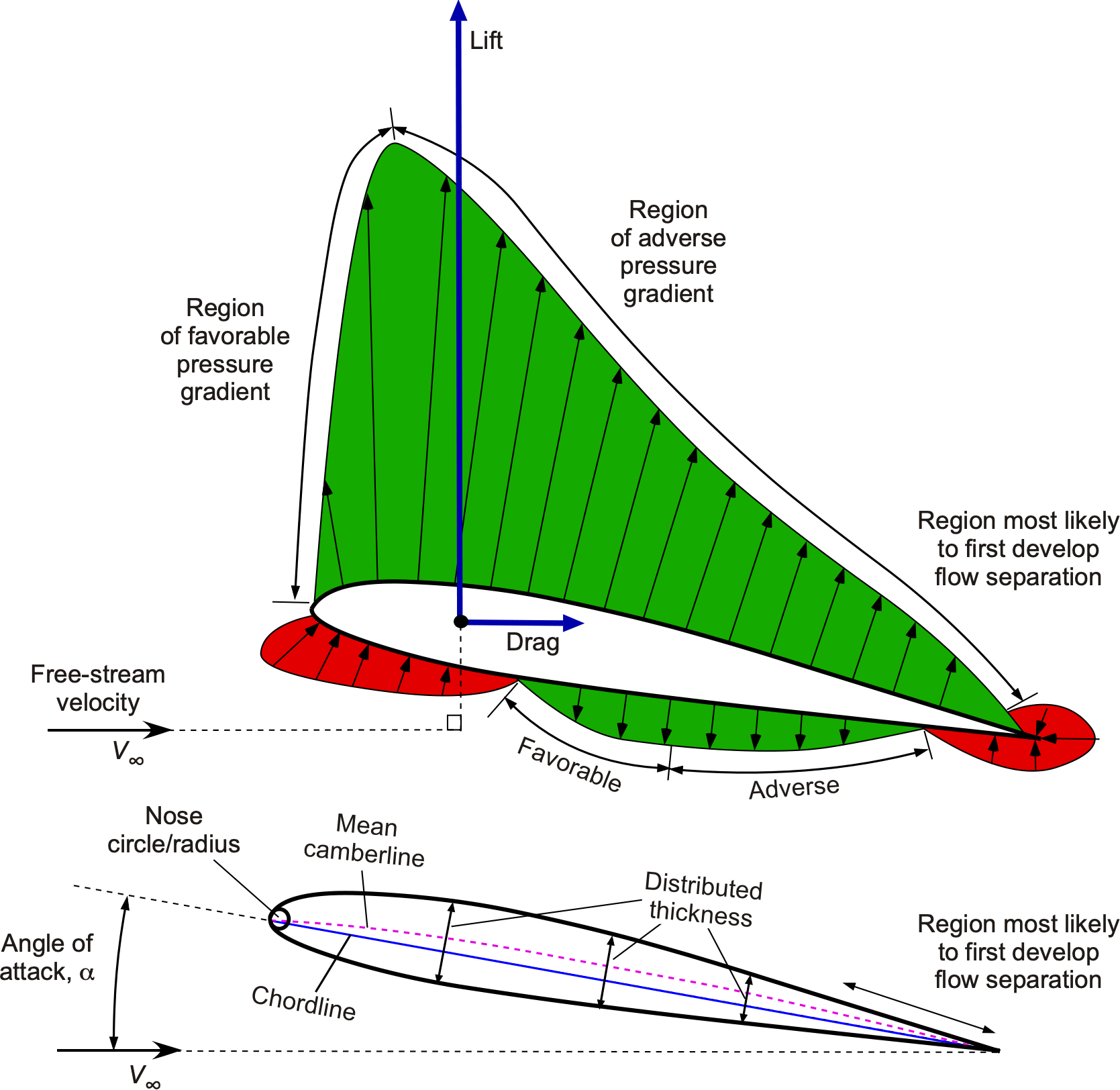
Use a solid line to indicate the chord line of the airfoil and a dashed line to indicate the mean camberline. See the figure.
Indicate the thickness distribution of the airfoil. See the figure.
Using the NACA method of airfoil construction then the thickness distribution is plotted perpendicular to the mean camberline.
Indicate the nose radius and explain why a nose radius is used on an airfoil. See the figure. The nose radius gives a smooth, geometrically defined nose shape.
Explain why an airfoil section is designed with a finite thickness at its trailing edge. For manufacturing reasons.
Indicate the angle of attack and explain why this airfoil will have a non-zero angle of attack. See the figure. The airfoil has a positive mean camberline, so the angle of attack must be depressed to a negative value to create a zero lift.
Indicate the lift and drag vectors acting on the airfoil. See the figure.
If $\alpha_0 = -2^{\circ}$ and $C_{l_{\alpha}} = 0.105$ per $^{\circ}$ , then calculate the lift coefficient. *** QuickLaTeX cannot compile formula:
{\color{red} C_l = C_{l_{\alpha}} \left( \alpha - \alpha_0 \right) = 0.105 \left( 10.0 - (-2.0)) \right) = 0.105 \times 12.0 = 1.26

*** Error message:
Missing } inserted.
leading text: ...-2.0)) \right) = 0.105 \times 12.0 = 1.26$

}
Indicate at least one region with a favorable pressure gradient and one region with an adverse pressure gradient on this airfoil. See the figure.
At the designated angle of attack, which region on the airfoil would be more likely to experience flow separation? Explain. See the figure. On the upper surface near the trailing edge where the adverse pressure gradient is significant.

Worked Example #2

Consider the following equations for the lift $L'$ and drag $D'$ forces acting on an airfoil as functions of the normal force $N'$ , the axial force $A'$ , and the angle of attack $\alpha$

$L' = N' \cos \alpha - A' \sin \alpha \quad \text{and} \quad D' = N' \sin \alpha + A' \cos \alpha$

Using these equations, derive expressions for $N'$ and $A'$ in terms of $L'$ , $D'$ , and $\alpha$ .

To find $N'$ and $A'$ , we start with the given equations, i.e.,

$L' = N' \cos \alpha - A' \sin \alpha \quad \text{and} \quad D' = N' \sin \alpha + A' \cos \alpha$

Multiply the first equation by $\cos \alpha$ and the second by $\sin \alpha$ , giving

$L' \cos \alpha = N' \cos^2 \alpha - A' \sin \alpha \cos \alpha \quad \text{and} \quad D' \sin \alpha = N' \sin \alpha \cos \alpha + A' \sin^2 \alpha$

Adding these equations gives

$L' \cos \alpha + D' \sin \alpha = N' (\cos^2 \alpha + \sin^2 \alpha)$

Using the identity $\cos^2 \alpha + \sin^2 \alpha = 1$ gives

$N' = L' \cos \alpha + D' \sin \alpha$

Now, multiply the first equation by $\sin \alpha$ and the second by $\cos \alpha$ giving

$L' \sin \alpha = N' \cos \alpha \sin \alpha - A' \sin^2 \alpha \quad \text{and} \quad D' \cos \alpha = N' \sin \alpha \cos \alpha + A' \cos^2 \alpha$

Subtracting these equations gives

$L' \sin \alpha - D' \cos \alpha = -A' (\sin^2 \alpha + \cos^2 \alpha)$

Using $\sin^2 \alpha + \cos^2 \alpha = 1$ , then

$A' = D' \cos \alpha - L' \sin \alpha$

Therefore,

$N' = L' \cos \alpha + D' \sin \alpha \quad \text{and} \quad A' = D' \cos \alpha - L' \sin \alpha$

Worked Example #3

Assuming a lift-curve slope for the linear range is 0.11 per degree angle of attack, i.e., $C_{l_{\alpha}} = 0.11$ per deg., then calculate the lift coefficients at 2, 6, and 10 deg. angle of attack for (a) A symmetric airfoil; (b) A positively cambered airfoil with a zero lift angle of attack of -1.2 deg; (c) A reflexed airfoil with a zero lift angle of attack of 1.7 deg.

(a) The equation for the lift coefficient in the linear range is given by

$C_l = C_{l_{\alpha}} \left( \alpha - \alpha_0 \right)$

In this case, $C_l = C_{l_{\alpha}} \left( \alpha - \alpha_0 \right) = 0.11\left( \alpha - 0 \right) = 0.11 \alpha$ .

For 2 $^{\circ}$ , then $C_l$ = 0.22
For 6 $^{\circ}$ , then $C_l$ = 0.66
For 10 $^{\circ}$ , then $C_l$ = 1.1

(b) $C_l = C_{l_{\alpha}} \left( \alpha - \alpha_0 \right) = 0.11\left( \alpha - (-1.2)\right) = 0.11\left( \alpha + 1.2 \right)$

For 2 $^{\circ}$ , then $C_l$ = 0.352
For 6 $^{\circ}$ , then $C_l$ = 0.792
For 10 $^{\circ}$ , then $C_l$ = 1.232

(c) $C_l = C_{l_{\alpha}} \left( \alpha - \alpha_0 \right) = 0.11\left( \alpha - 1.7 \right)$

For 2 $^{\circ}$ , then $C_l$ = 0.033
For 6 $^{\circ}$ , then $C_l$ = 0.473
For 10 $^{\circ}$ , then $C_l$ = 0.913

Worked Example #4

Given that the pressure coefficient $C_p$ distribution over a 2-dimensional body of chord $c$ is described by $C_p = -4(1 - x/c)$ on the upper surface of the body and $C_p = (1-x/c)$ on the lower surface of the body, then calculate (by integration): (a) The lift coefficient acting on the body; (b) The pitching moment coefficient on the body about its leading edge.

The pressure distribution in this question is given in analytic form to solve the problem without any numerical integration. However, a MATLAB code is provided to check this answer by numerical integration.

(a) The lift coefficient $C_l$ is given by

$C_l = \int_0^1 \Delta C_p d(x/c) = \int_0^1 (C_{p_{l}} - C_{p_{u}}) d \overline{x}$

In this case we can see that $C_{p_{l}} - C_{p_{u}} = 5 (1 - \overline{x})$ so the integral for $C_l$ becomes

$C_l = \int_0^1 5 (1 - \overline{x}) d\overline{x} = 5 \left[ \overline{x} - \frac{\overline{x}^2}{2} \right]_0^1 = 2.5$

(b) The pitching moment about the leading edge is

$C_{m_{le}} = -\int_0^1 \Delta C_p \, (x/c) \, d(x/c) = -\int_0^1 \Delta C_p \, \overline{x} \, d\overline{x}$

Substituting $\Delta C_p= 5 (1 - \overline{x})$ then

$C_{m_{le}} = -\int_0^1 5 (1 - \overline{x}) \overline{x} \, d\overline{x} = 5 \left[ \frac{\overline{x}^2}{2} - \frac{\overline{x}^3}{3} \right]_0^1 = -\frac{5}{6} = -0.833$

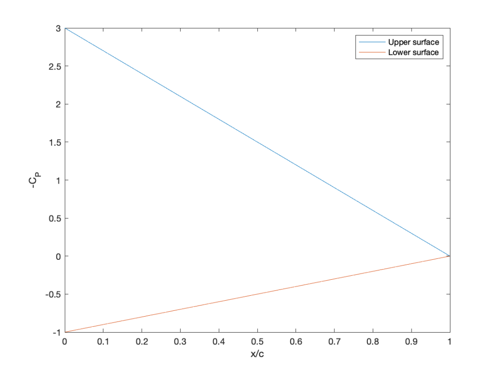
Here is some MATLAB code to cross-check the results and plot the pressure distribution.
clc
figure
axis([0.0 1.0 1.0 5.0])
x = linspace(0.0,1.0,100); %set the range of x/c values
cpu = -4.*(1-x);
cpl = 1.*(1-x);
dcp = cpl-cpu;
trapz(x,dcp) % check to find the section cl using the trapezoidal rule
dcpx = -dcp.*x;
trapz(x,dcpx) % check to find the section cl_le using the trapezoidal rule
plot(x,-cpu);hold on
plot(x,-cpl)
xlabel(‘x/c’)
ylabel(‘-C_P’)
legend(‘Upper surface’, ‘Lower surface’)

Worked Example #5

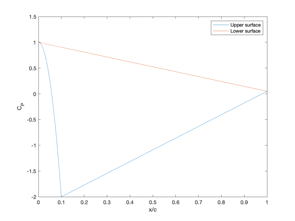
The pressure coefficient $C_p$ distribution over a 2-dimensional body of chord $c$ operating at a low angle of attack is described by

$C_{p_{u}} = 1 - 300 \left( \frac{x}{c} \right)^2 \quad \mbox{for $0 \le x/c \le 0.1$}$

$C_{p_{u}} = -2.2277 + 2.2777 \left( \frac{x}{c} \right) \quad \mbox{for $0.1 < x/c \le 1.0$}$

$C_{p_{l}} = 1 - 0.95 \left( \frac{x}{c} \right) \mbox{for $0.0 \le x/c \le 1.0$}$

(a) Use MATLAB to plot the pressure coefficient distribution. (b) Calculate the lift coefficient by analytic integration. (c) Calculate the lift coefficient in MATLAB by numerical integration.

(a) The pressure distribution looks like this (see the last part of the answer for the code):

(b) The lift coefficient $C_l$ is given by

$C_l = \int_0^1 \Delta C_p \, d(x/c) = \int_0^1 (C_{p_{l}} - C_{p_{u}}) \, d \overline{x}$

which for this problem, we can split it into two integrals, namely

$C_l = \int_0^{0.1} (C_{p_{l}} - C_{p_{u}}) d \overline{x} + \int_{0.1}^1 (C_{p_{l}} - C_{p_{u}}) d \overline{x} = C_{l_{1}} + C_{l_{2}}$

Taking the first integral gives

$C_{l_{1}} = \int_0^{0.1} (C_{p_{l}} - C_{p_{u}}) d \overline{x} = \int_0^{0.1} \big( \left( 1 - 0.95 \overline{x} \right) - \left( 1 - 300 \overline{x} ^2 \right) \big) d \overline{x}$

and so

$C_{l_{1}} = \int_0^{0.1} \left( 300 \overline{x} ^2 - 0.95 \overline{x} \right) d \overline{x} = \Bigg[ 100 \overline{x}^3 - 0.475 \overline{x}^2 \Bigg]_{0}^{0.1} = 0.09525$

Taking the second integral gives

$C_{l_{2}} = \int_{0.1}^{1} (C_{p_{l}} - C_{p_{u}}) d \overline{x} = \int_{0.1}^{1} \big( \left( 1 - 0.95 \overline{x} \right) - \left( -2.2277 + 2.2777 \overline{x} \right) \big) d \overline{x}$

and so

$C_{l_{2}} = \int_{0.1}^{1} 3.2277 \left( 1- \overline{x} \right) d \overline{x} = \Bigg[ 3.2277 \left( \overline{x} - \frac{\overline{x}^2}{2} \right) \Bigg]_{0.1}^{1} = 1.307$

Therefore,

$C_{l} = C_{l_{1}} + C_{l_{2}} = 0.09525 + 1.307 = 1.4025$

(c) The MATLAB code, which uses numerical integration, gives $C_l$ = 1.4025, so the results of the two methods agree.

clc
figure
axis([0.0 1.0 1.0 5.0])
x1 = linspace(0,0.1,500);
x2 = linspace(0.1,1,500);
cpu_1 = 1.-300*x1.^2;
cpu_2 = -2.2277 + 2.2777.*x2;
x = [x1 x2];
cpu = [cpu_1 cpu_2];
cpl = (1.0-0.95*x);
dcp = cpl-cpu;
trapz(x,dcp) % section cl using the trapezoidal rule
plot(x,cpu);hold on
plot(x,cpl)
xlabel(‘x/c’)
ylabel(‘C_P’)
legend(‘Upper surface’, ‘Lower surface’)

Worked Example #6

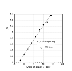
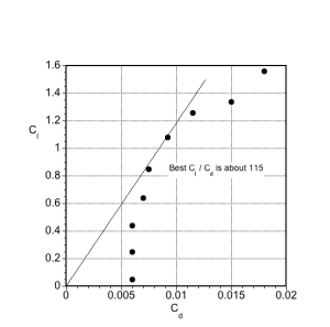
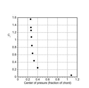
As shown in the table below, the lift, drag, and pitching moment coefficient measurements for a NACA 2412 airfoil will be used to calculate specific derived aerodynamic quantities. First, determine the values of the following parameters: (a) Lift curve slope; (b) Zero-lift angle of attack; (c) Drag polar (as a plot); (d) The best lift-to-drag ratio; (e) Center of pressure location (as a plot).

$\alpha$ (deg.)	$C_l$	$C_d$	$C_{m_{1/4}}$
-2	0.05	0.006	-0.042
0	0.25	0.006	-0.040
2	0.44	0.006	-0.038
4	0.64	0.007	-0.036
6	0.85	0.0075	-0.036
8	1.08	0.0092	-0.036
10	1.26	0.0115	-0.034
12	1.43	0.015	-0.030
14	1.56	0.0186	-0.025

(a) Lift curve slope = $\displaystyle{\frac{d C_l }{d \alpha}}$ = $C_{l_{\alpha}}$ = 0.0949 per degree, as shown on plot below. The slope is obtained using a least-squares linear fit.

(b) Zero-lift angle of attack = $\alpha_0$ = -2.75 degrees, as shown on the same plot.

(c) Drag polar (as a plot), as per the plot shown below

(d) The best lift-to-drag ratio = $(C_l/C_d)_{\rm max}$ , which is about 115 in this case and not untypical for a two-dimensional airfoil.

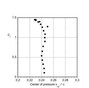
(e) Center of pressure location, as shown in the plot below.

Worked Example #7

Examine the attached graph, which shows the aerodynamic coefficients for a NACA 66 $_1$ -212 airfoil section.
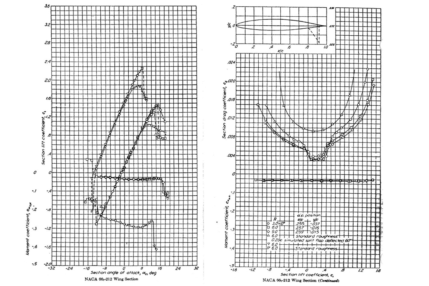For the flap-up case then, estimate the following values for a Reynolds number of $6 \times 10^6$ (you may also want to annotate the graph):
(a) The zero-lift angle of attack.
(b) The maximum lift coefficient.
(c) The stall angle of attack.
(d) The minimum drag coefficient. Also, why is there a “bucket” in the drag curve?
(e) The lift-to-drag ratio at an angle of attack of 8 degrees.
(f) The minimum drag coefficient with roughness. Explain why the drag of the airfoil increases with the application of roughness.

(a) The zero-lift angle of attack. Answer: -1.5 $^{\circ}$ .

(b) The maximum lift coefficient. Answer: 1.45.

(c) The stall angle of attack. Answer: 15 $^{\circ}$

(d) The minimum drag coefficient. Answer: 0.003. There is a “bucket” in the drag curve because this airfoil experiences extended regions of laminar boundary layer flow between certain (low) angles of attack. Such characteristics are typical for certain airfoil sections, especially those used on sailplanes.

(e) The lift-to-drag ratio at an angle of attack of 8 degrees. Answer: 92

(f) The minimum drag coefficient with roughness. Answer: About 0.009. Surface roughness eliminates the run of the laminar boundary layer over the front part of the airfoil and makes it turbulent, increasing skin friction drag. You can think of roughness as equivalent to using some medium-grade sandpaper on the surface. Airfoils and wings for airplanes are often tested in the wind tunnel with smooth and rough surfaces, the idea being to simulate the effects of wear and tear on the wing after the airplane has been in operational service. Some airfoils, like the one given in this example, are particularly sensitive to the effects of surface roughness.

Worked Example #8

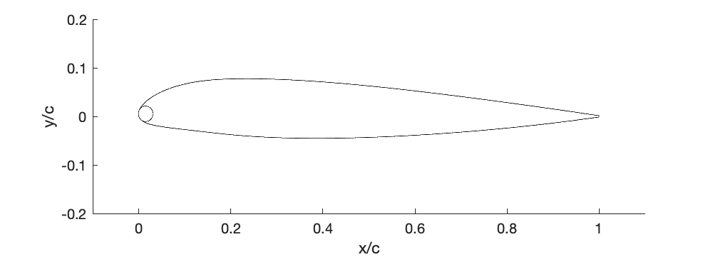
Modify the MATLAB NACA 230-series camberline airfoil generator code given in the e-book to plot some of the NACA 231 series reflexed airfoils. Why is reflex camber used on an airfoil? You should plot the NACA 23112 and NACA 23118 shapes, but you may plot different shapes in the series if you wish.

The camberline for the NACA 3-digit 231-series reflex airfoils is given by

$\frac{y_{c}}{c} = \frac{k_1}{6} \left[ \left( \frac{x}{c} - m \right)^3 - \frac{k_2}{k_1} \left( 1 - m\right)^3 \, \frac{x}{c} - m^3 \, \frac{x}{c} + m^3 \right] ~\mbox{from $x/c \le m$}$

and

$\frac{y_{c}}{c} = \frac{k_1}{6} \left[ \frac{k_2}{k_1} \left( \frac{x}{c} - m \right)^3 - \frac{k_2}{k_1} \left( 1 - m \right)^3 \, \frac{x}{c} - m^3 \, \frac{x}{c} + m^3 \right]~\mbox{from $m< x/c \le 1.0$}$

where $m = 0.217$ , $p = 0.15$ , $k_1 =15.793$ , and $k_2/k_1 = 0.00677$ .

The MATLAB code below will draw a NACA 231-series reflexed airfoil. Remember that reflex camber aims to reduce the pitching moment on the airfoil.

t = 0.12;
m = 0.217; %location of maximum camber
k1 = 15.793; %constant
k2k1 = 0.006770;
r = 1.1019.*(t^2); %radius of leading edge circle
x1 = linspace(r/3,m,round(m.*500)); %x coordinates nose circle to m
x2 = linspace(m,1,round((1-m).*500)); %x coordinates m to 1
y_cam_1 = (k1./6).*(((x1-m).^3)-k2k1*((1-m).^3)*x1-(m.^3)*x1+m.^3); %camber line y coord 0 to m
y_cam_2 = (k1./6).*((k2k1*(x2-m).^3)-((k2k1*(1-m).^3)*x2)-((m.^3)*x2)+(m.^3)); %camber line y coord m to 1
x = [x1 x2]; %merged x coordinates
y_cam = [y_cam_1 y_cam_2]; %merged y camber coordinates
dy_cam_1 = (k1./6).*((3.*(x1-m).^2)-k2k1*(1-m).^3-(m.^3)); %derivative of camber line 0 to m
dy_cam_2 = (k1./6).*((3.*k2k1*(x2-m).^2)-k2k1.*(1-m).^3-m.^3).*ones(1,length(x2)); %derivative of camber line m to 1
dy_cam = [dy_cam_1 dy_cam_2]; %merged derivative of camber line
theta = atan(dy_cam); %slope of camber line
y_t = 5.*t.*((0.29690.*sqrt(x))-(0.12600.*x)-(0.35160.*(x.^2)) +(0.28430.*(x.^3))-(0.10150.*(x.^4))); %thickness equation
x_upper = x-(y_t.*sin(theta)); %x coordinates of upper surface
x_lower = x+(y_t.*sin(theta)); %x coordinates of lower surface
y_upper = y_cam+(y_t.*cos(theta)); %y coordinates of upper surface
y_lower = y_cam-(y_t.*cos(theta)); %y coordinates of lower surface
%end points to close off trailing edge
x_end_up = x_upper(end);
x_end_low = x_lower(end);
y_end_up = y_upper(end);
y_end_low = y_lower(end);
dy_cam_005 = (1./6).*k1.*(3.*(0.005-m).^2)-k2k1*((1-m).^3-(m.^3));
%derivative of camber line at x = 0.005theta_005 = atan(dy_cam_005); %slope of camber line at x = 0.005

The shapes of the NACA 23112 and NACA 23118 are shown below.

Worked Example #9

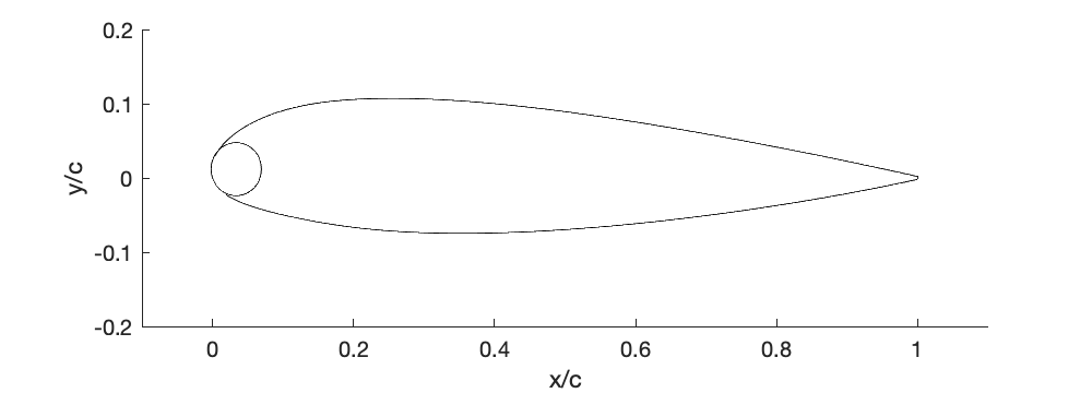
Lift, drag, and pitching moment measurements for a NACA 0012 airfoil are given in the table below. They will be used to calculate specific derived aerodynamic quantities for further analysis. As part of the analysis, you are asked to determine the following: (a) Lift curve slope (in the attached flow regime). (b) The zero-lift angle of attack. (c) Drag polar (as a plot). (d) The best lift-to-drag ratio. (e) Center of pressure location (as a plot). (f) Aerodynamic center location.

Angle of attack	C_l	C_d	C_m
0	0	0.00662	0
1	0.1096	0.0067	0.0006
2	0.2182	0.00693	0.0013
3	0.3254	0.00736	0.0024
4	0.4309	0.008	0.0038
5	0.5365	0.00881	0.0054
6	0.6509	0.00976	0.0057
7	0.7743	0.01085	0.0057
8	0.9006	0.01203	0.0041
9	0.9957	0.01328	0.0046
10	1.0836	0.01466	0.0046
11	1.1729	0.01627	0.0079
12	1.2585	0.01817	0.0113
13	1.3343	0.02057	0.0157
14	1.3928	0.02328	0.0221
15	1.4322	0.02739	0.0284
16	1.4511	0.0345	0.0315
17	1.4508	0.04615	0.0287
18	1.4004	0.06732	0.0186
19	1.2739	0.10324	0.0001

(a) Lift curve slope (in the attached flow regime). The lift-curve slope is obtained by fitting a straight line (least-squares fit) through the measurements at a low angle of attack. In this case $dC_l/d\alpha$ or $C_{l_{\alpha}}$ = 0.107 per degree angle of attack.

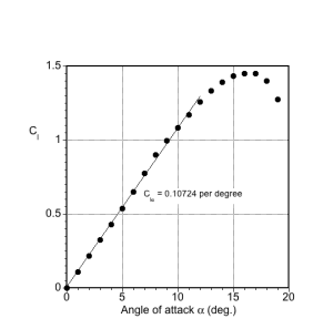
(b) Zero-lift angle of attack. This is a symmetric airfoil, so the zero lift angle of attack $\alpha_0 = -0.02$ is based on the linear fit and so effectively zero degrees as expected.

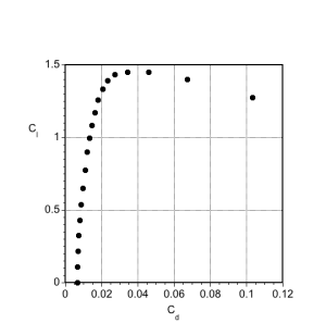
(c) Drag polar (as a plot). The drag polar is a plot of the lift coefficient $c_l$ versus the drag coefficient $C_d$ . The advantage of this presentation is that a straight line running from the origin of the graph at (0,0) to any point on the polar is the lift-to-drag ratio $C_l/C_d$ . The best lift-to-drag ratio is when this line is just tangent to the polar curve.

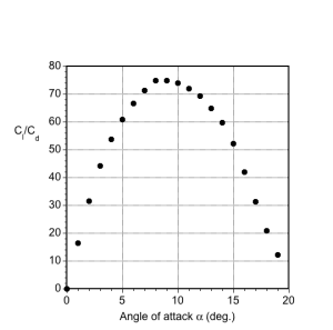
(d) The best lift-to-drag ratio. Another way to find the lift-to-drag ratio is to plot this ratio as a function of the angle of attack $\alpha$ or $C_l$ . In this case, the best lift-to-drag ratio is about 75, typical for a good airfoil section.

(e) Center of pressure location (as a plot). The center of pressure can be calculated using

$\frac{x_{\rm cp}}{c} = \frac{1}{4} - \frac{C_{m_{1/4}}}{C_{l}}$

The moments are given in the data file about the 1/4-chord. The center of pressure is a function of the lift coefficient (and hence also the angle of attack), so it is not a fixed point and a convenient concept to use in aerodynamics. Therefore, the center of pressure to resolve the forces and moments is used sparingly in practice even though the pitching moment is zero about this point.

(f) Aerodynamic center location. By definition, the aerodynamic center is the point where the moment is independent of $C_{l}$ . The moments in the data file are given about the 1/4-chord (generally, this is the default), so the aerodynamic center is calculated using

$\frac{x_{ac}}{c} = \frac{1}{4} - \frac{d C_{m_{1/4}}}{dC_{l}}$

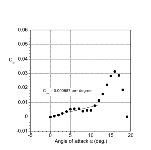
We can obtain the value of $dC_{m_{1/4}}/d C_l$ using

$\frac{d C_{m_{1/4}} }{ d C_l} = \left( \frac{ d C_{m_{1/4}}}{d \alpha}\right) \left( \frac{d \alpha}{d C_{l}}\right)$

So, we need the lift-curve slope and the slope of the moment curve (again, in the low angle of attack regime). In this case, we have

$\frac{x_{ac}}{c} = \frac{1}{4} - \frac{0.000687}{0.107} = 0.2436$

which, unlike the center of pressure, is a fixed point. For most airfoils at low Mach numbers, the aerodynamic center is close to 1/4-chord.

Worked Example #10

An airplane wing has a semi-span of 9.5m. The wing’s root chord at the aircraft’s centerline is 1.5 m. This constant chord extends to 3 m from the root at the centerline, followed by a linearly tapered part from that point to a tip chord of 1.2 m. For this wing, calculate (a) The wing area, (b) The aspect ratio, and (c) The mean aerodynamic chord (MAC).

(a) We can split the area calculation of each wing panel into two parts, i.e., $S = S_1 + S_2$ , with the first part ending at a distance $y = y_b$ = 3 m from the wing root and the second part running to the wing tip. For the first (rectangular) part of the wing panel, then

$S_1 = 2 (c_r y_b) = 2 \times (1.5 \times 3) = 9.0~\mbox{m$^2$}$

remembering to multiply by two because there are two wing panels. For the second (tapered) part, then

$S_2 = 2 \left( \frac{c_r + c_t}{2} \right) \left( s - y_b \right) = 2 \left( \frac{1.5 + 1.2}{2} \right) \left( 9.5 - 3.0 \right) = 17.55~\mbox{m$^2$}$

Again, the factor of 2 denotes two wing panels. Therefore, the total wing area is

$S = S_1 + S_2 = 9.0 + 17.55 = 26.55~\mbox{m$^2$}$

(b) The aspect ratio $A\!R$ of this wing is

$A\!R = \frac{b^2}{S} = \frac{4s^2}{S} = \frac{4 \times 9.5^2}{26.55} = 13.6$

(c) The MAC is given by

${\rm MAC} \equiv \overline{\overline{c}} = \frac{2 \displaystyle{\int_{0}^{s} c^2 dy}}{S}$

In this case, we have two parts to the wing panel, the first part with a constant chord ending at a distance $y = y_b$ = 3 m from the wing root. We need to evaluate the term

$\int_{0}^{s} c^2 dy = \int_{0}^{y_b} c^2 dy + \int_{y_b}^{s} c^2 dy$

The first term is easy because $c = c_r$ , so

$\int_{0}^{y_b} c^2 dy = \int_{0}^{y_b} c_r^2 dy = c_r^2 y_b = (1.5)^2 \, 3.0 = 6.75~\mbox{m${^3}$}$

The second term involves the tapered part of the wing, so for $y \ge y_b$ , the chord variation is

$c(y) = c_r + \left( \frac{c_t - c_r}{s-y_b} \right) ( y - y_b )$

If we let

$A = \left( \frac{c_t - c_r}{s-y_b} \right)$

then

$c^2 = \left( c_r + A ( y - y_b ) \right)^2 =\left( (c_r - A y_b) + Ay \right)^2 = (c_r - A y_b)^2 + 2 A (c_r - Ay_b) y + A^2 y^2$

and if we let

$B = c_r - A y_b$

then

$c^2 = B^2 + 2 AB y + A^2 y^2$

Therefore, we have that

$\int_{y_b}^{s} c^2 dy = \int_{y_b}^{s} \left( B^2 + 2 AB y + A^2 y^2 \right) dy = \left[ B^2 y + ABy^2 + \frac{A^2}{3} y^3 \right]_{y_b}^{s}$

Introducing the limits of integration and evaluating all of the terms gives

$\int_{y_b}^{s} c^2 dy = 11.9~\mbox{m${^3}$}$

and so the MAC is

$\overline{\overline{c}}= \frac{2 \displaystyle{\int_{0}^{s} c^2 dy}}{S} = \frac{ \displaystyle{ 2 \int_{0}^{y_b} c^2 dy + 2 \int_{y_b}^{s} c^2 dy}}{S} = \frac{2 (6.75 + 11.9)}{26.55} = 1.405~\mbox{m}$

Worked Example #11

A wing has an aspect ratio of 12. The chord of the wing varies smoothly and continuously outward from the centerline of the aircraft according to

$c(y) = 1 - 0.32 \left( \frac{y}{b} \right)~\mbox{in units of meters}$

For this wing, then calculate the wing span and the wing area.

The area of the wing $S$ is

$S = 2 \int_{0}^{s} c \, dy$

The chord for this wing is

$c(y) = 1 - 0.32 \left( \frac{y}{b} \right) = 1 - 0.32 \left( \frac{y}{2s} \right) = 1 - 0.16 \left( \frac{y}{s} \right)$

and substituting for the chord distribution $c(y)$ gives

$S = 2 \int_{0}^{s} c \, dy = 2 \int_{0}^{s} \left( 1.0 - 0.16 \left( \frac{y}{s} \right) \right) dy$

Introducing the limits of integration gives

$S = 2 \left[ 1.0 y - \frac{0.08}{s} y^2 \right]_0^s = 2(s - 0.08s) = 1.84s$

noting that $b = 2 s$ .

The aspect ratio $A\!R$ of this wing is

$A\!R = \frac{b^2}{S} = \frac{4s^2}{S} = \frac{4s^2}{1.84s} = 2.174 s$

Therefore, solving for the span $b$ for an aspect ratio of 12 gives

$b = 2s = 2 \left( \frac{A\!R}{2.174}\right) = \frac{2 \times 12}{2.174} = 11.04~\mbox{m}$

and so the area of this wing is

$S = 1.84 s = 1.84/b/2= 1.84 \times 5.52= 10.157~\mbox{m$^2$}$

Worked Example #12

A sailplane wing has a span of 15 m. The root chord at the aircraft’s centerline is 1 m, and the wing tapers linearly from the root to the tip with a tip chord of 0.5 m. For this wing, calculate (a) The wing area, (b) The aspect ratio, and (c) The mean aerodynamic chord (MAC).

We are given the wing’s span (distance from the left wing tip to the right wing tip) $b$ , the root chord $c_r$ , and the tip chord $c_t$ . The wing panel is tapered linearly, i.e., each of the left and right-wing panels of a trapezoidal shape, so the area of one wing panel will be half of the average chord times the semi-span $s$ . Therefore, with the two wing panels, the area $S$ is

$S = 2 \left( \frac{c_t + c_r}{2} \right) s = 2 \left( \frac{1.0 + 0.5}{2} \right) \frac{15}{2} = 11.25~\mbox{m$^2$}$

Notice that we can also work with general expression for the chord $c$ as a function of distance $y$ from the wing root to the right wing tip (a distance equal to the semi-span $s$ ) will be

$c(y) = c_r + A y$

where $A$ is a measure of the taper. The boundary conditions are that $c(0) = c_r$ and $c(s) = c_t$ . Therefore,

$c_t = c_r + A s$

so solving for $A$ gives

$A = \frac{c_t - c_r}{s}$

and so

$c(y) = c_r + \left( \frac{c_t - c_r}{s} \right) y$

We can check that this expression is indeed correct by substituting $y = 0$ and $y = s$ . The area of the wing $S$ will then be

$S = 2 \int_{0}^{s} c dy$

and substituting for the chord distribution $c(y)$ gives

$S = 2 \int_{0}^{s} c dy = 2 \int_{0}^{s} \left( c_r + A y\right) dy$

Therefore,

$S = 2 \left[ c_r y + \frac{A y^2}{2} \right]_0^s = c_r s + \frac{As^2}{2} = c_r s + \left(\frac{c_t - c_r}{s} \right) \frac{s^2}{2} = \left( \frac{c_r + c_t}{2} \right) s$

i.e., just the standard formula for the area of a trapezoid we used previously.

The aspect ratio $A\!R$ of this wing is

$A\!R = \frac{b^2}{S} = \frac{15^2}{11.25} = 20$

The MAC is given by

${\rm MAC} = \overline{\overline{c}} = \frac{2 \displaystyle{\int_{0}^{s} c^2 dy}}{S}$

In this case, then

$c(y) = c_r + \left( \frac{c_t - c_r}{s} \right) y$

so

$\int_{0}^{s} c^2 dy = \int_{0}^{s} \left( c_r + \left( \frac{c_t - c_r}{s} \right) y \right)^2 dy = \int_{0}^{s} \left( c_r^2 + 2\left( \frac{c_t - c_r}{s} \right) c_r y + \left( \frac{c_t - c_r}{s} \right)^2 y^2 \right) dy$

Integrating gives

$\int_{0}^{s} c^2 dy = \left[ c_r^2 y + \left( \frac{c_t - c_r}{s} \right) c_r y^2 + \frac{1}{3} \left( \frac{c_t - c_r}{s} \right)^2 y^3 \right]_0^s$

so

$\overline{\overline{c}} = c_r^2 s + \left(c_t - c_r \right) c_r s + \frac{1}{3} \left( c_t - c_r \right)^2 s = c_t c_r s + \frac{1}{3} \left( c_t - c_r \right)^2 s$

Therefore, the MAC for this wing is

$\overline{\overline{c}} = \frac{2 \left( (0.5 \times 1.0\times 7.5) + \displaystyle{\frac{(-0.5)^2}{3}} 7.5) \right) }{11.25} = 0.778~\mbox{m}$

Worked Example #13

A wing of a span of 30 ft has an elliptical wing planform with a root chord of 6 ft. Calculate for this wing: (a) The wing (planform) area; (b) The aspect ratio of this wing; (c) The mean aerodynamic chord (MAC).

(a) The chord, in this case for an elliptical planform shape, is

$c(y) = c_0\sqrt{ 1 - \left( \frac{y}{s} \right)^2 }$

where $c_0$ is the root chord. The area of the wing $S$ is

$S = 2 \int_{0}^{s} c \, dy$

and so substituting for the chord gives

$S = 2 \int_{0}^{s} c_0\sqrt{ 1 - \left( \frac{y}{s} \right)^2 } \, dy = 2 c_0 \int_{0}^{s} \sqrt{ 1 - \left( \frac{y}{s} \right)^2 } \, dy$

This is a standard integral, so

$S = 2 c_0 \left[ \frac{1}{2} \left( y \sqrt{1 - \frac{y^2}{s^2} } + s \sin^{-1} \left( \frac{y}{s} \right) \right) \right]_0^s = c_0 \left[ y \sqrt{1 - \frac{y^2}{s^2} } + s \sin^{-1} \left( \frac{y}{s} \right) \right]_0^s = \frac{\pi c_0 s}{2}$

Therefore, the area of the elliptical wing is

$S = \frac{\pi c_0 s}{2} = \frac{ \pi \times 6.0 \times 15.0}{2} = 141.372~\mbox{ft$^2$}$

(b) The aspect ratio $A\!R$ for this wing is

$A\!R = \frac{b^2}{S} = \frac{4s^2}{S} = \frac{4 \times 15.0^2}{141.372} = 6.366$

(c) The MAC is given by

${\rm MAC} = \overline{\overline{c}} = \frac{2 \displaystyle{\int_{0}^{s} c^2 dy}}{S}$

In this case, then

$c(y) = c_0\sqrt{ 1 - \left( \frac{y}{s} \right)^2 }$

so

$c(y)^2 = c_0^2 \left( 1 - \left( \frac{y}{s} \right)^2 \right)$

This means that for this elliptical wing, then

$\int_{0}^{s} c^2 dy = \int_{0}^{s} c_0^2 \left( 1 - \left( \frac{y}{s} \right)^2 \right) dy = c_0^2 \int_{0}^{s} \left( 1 - \left( \frac{y}{s} \right)^2 \right) dy = c_0^2 \left[ y - \frac{y^3 }{3s^2}\right]_0^s = \frac{2}{3} c_0^2 s$

$\overline{\overline{c}} = \frac{2 \displaystyle{\int_{0}^{s} c^2 dy}}{S} = \frac{ \left( \displaystyle{\frac{4}{3}} \right)c_0^2 s}{S} = \frac{ \left( \displaystyle{\frac{4}{3}} \right)6.0^2 \, 15.0}{141.372} = 5.093~\mbox{m}$

Worked Example #14

The drag coefficient $C_D$ of a particular airplane is described by the equation

$C_D = 0.035 + \left( \frac{1.35}{\pi \, A\!R} \right) {C_L}^2$

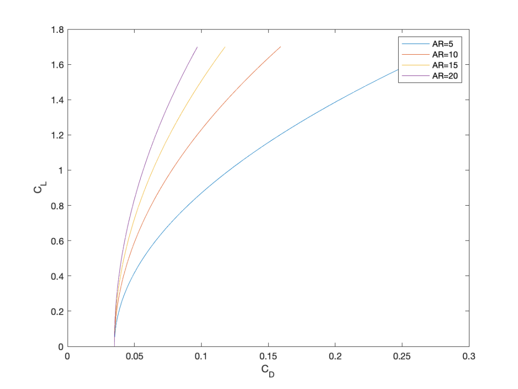
where $A\!R$ is the aspect ratio of the wing. Plot the drag polars for this airplane design for wing aspect ratios of 5, 10, 15, and 20. In each case, determine the best lift-to-drag ratio and the conditions under which this occurs. Assume that the maximum attainable lift coefficient of the wing is 1.7. Comment on your results.

The MATLAB code is listed below:

clc
figure
axis([0.0 0.3 0.0 2.0])
CL = linspace(0.0,1.7,100); %set the range of CL values for A\!R = 5:5:20 % set the range of AR values
CD = 0.035+1.35*CL.^2/pi/AR;
plot(CD,CL);hold on
end
legend(‘AR=5′,’AR=10′,’AR=15′,’AR=20’);
xlabel(‘C_D’)
ylabel(‘C_L’)

The plot below shows the polars produced by the MATLAB code. Notice the significant effects of aspect ratio $A\!R$ on the curve. The lower aspect ratio wing always gives higher induced drag (i.e., “drag due to lift”), so the drag increases more quickly with increasing lift coefficient.

We are asked to find the best lift-to-drag ratio for each wing and the lift coefficient at which this occurs. It is possible to do that from the graph or numerically within MATLAB, but it can also be done analytically. The drag coefficient is given by

$C_D = 0.035 + \left( \frac{1.35}{\pi \, A\!R} \right) {C_L}^2 = A + B {C_L}^2$

This means that

$\frac{C_D}{C_L} = \frac{A}{C_L} + B C_L$

Differentiating gives

$\frac{d (C_D/C_L)}{d (C_L)} = -\frac{A}{{C_L}^2} + B = 0 \mbox{~~for a maximum or minimum}$

Therefore, solving for $C_L$ at this condition gives

$C_L = \sqrt{ \frac{A}{B} } = \sqrt{ \frac{0.035 \pi \, A\!R}{1.35} }$

This will be the lift coefficient used to obtain the maximum lift-to-drag ratio.

For $A\!R = 5$ then the $C_L$ for best $C_L/C_D$ is

$C_L = \sqrt{ \frac{0.035 \pi \, A\!R}{1.35} } = \sqrt{ \frac{0.035 \times \pi \times 5 }{1.35} } = 0.638$

The corresponding $C_L/C_D$ ratio is

$\frac{C_L}{C_D} = \frac{C_L}{C_D} = \frac{C_L}{A + B {C_L}^2} = \frac{C_L}{0.035 + (1.35/\pi/AR){C_L}^2}$

and substituting values gives and a $C_L$ of 0.638 gives the best lift-to-drag ratio for this wing as

$\frac{C_L}{C_D} = \frac{C_L}{0.035 + (1.35/\pi/AR){C_L}^2} = \frac{0.638} {0.035 + (1.35/\pi/5)0.638^2} = 9.12$

For $A\!R = 10$ then the $C_L$ for best $C_L/C_D$ is

$C_L = \sqrt{ \frac{0.035 \pi \, A\!R}{1.35} } = \sqrt{ \frac{0.035 \times \pi \times 10 }{1.35} } = 0.903$

and substituting values with $C_L$ = 0.903 gives the best lift-to-drag ratio for this wing as

$\frac{C_L}{C_D} = \frac{C_L}{0.035 + (1.35/\pi/AR){C_L}^2} = \frac{0.903}{0.035 + (1.35/\pi/10)0.903^2} = 12.89$

For $A\!R = 15$ then the $C_L$ for best $C_L/C_D$ is

$C_L = \sqrt{ \frac{0.035 \pi \, A\!R}{1.35} } = \sqrt{ \frac{0.035 \times \pi \times 15 }{1.35} } = 1.105$

and substituting values with $C_L$ = 1.105 gives the best lift-to-drag ratio for this wing as

$\frac{C_L}{C_D} = \frac{C_L}{0.035 + (1.35/\pi/AR){C_L}^2} = \frac{1.105}{0.035 + (1.35/\pi/15)1.105^2} = 15.79$

For $A\!R = 20$ then the $C_L$ for best $C_L/C_D$ is

$C_L = \sqrt{ \frac{0.035 \pi \, A\!R}{1.35} } = \sqrt{ \frac{0.035 \times \pi \times 20 }{1.35} } = 1.276$

and substituting values with $C_L$ = 1.276 gives the best lift-to-drag ratio for this wing as

$\frac{C_L}{C_D} = \frac{C_L}{0.035 + (1.35/\pi/AR){C_L}^2} = \frac{1.276}{0.035+ (1.35/\pi/20)1.276^2} = 18.23$

The preceding results clearly show that the best lift-to-drag ratio increases with increasing aspect ratio. Also, the lift coefficient at which the best lift-to-drag ratio is obtained increases with increasing aspect ratio.

Worked Example #15

Consider a flying wing with a wing area of 210 m $2$ , an aspect ratio of 10, and Oswald’s efficiency factor of 0.90. The airfoil section on the wing has a profile drag coefficient of 0.015. The airplane’s mass is 50,000 kg. If the aircraft is flying at a density altitude of 3 km and the true airspeed is 230m/s, then calculate the total drag on the aircraft.

The air density at a density altitude of 3 km is 0.90925 kg m ${^{-3}}$ when using the ISA model. For vertical force equilibrium, the lift on the wing $L$ is equal to the weight of the aircraft, $W$ , i.e.,

$L = M g = 50,000 \times 9.81 = 490,500 ~{\mbox N}$

The lift is given by

$L = \frac{1}{2} \varrho V^2 S C_L$

so the operating lift coefficient of the wing is

$C_L = \frac{L}{ \frac{1}{2} \varrho V^2 S} = \frac{Mg }{ \frac{1}{2} \varrho V^2 S} = \frac{490,500 }{0.5 \times 0.90925 \times 230.0^2 \times 210.0} = 0.097$

The drag coefficient is given by

$C_D = C_{D_{0}} + \frac{{C_L}^2}{\pi \, AR e} = 0.015 + \frac{0.097^2}{\pi \times 10.0 \times 0.90} = 0.0153$

where the non-lifting part $C_{D_{0}} = 0.015$ , i.e., $C_{D_{0}} = C_{d_{0}}$ .

Therefore, the drag force is

$D = \frac{1}{2} \varrho V^2 S C_D = 0.5 \times 0.90925 \times 230.0^2 \times 210.0 \times 0.0153 = 77,271.6~\mbox{N}$

giving a lift-to-drag ratio of about 6, which seems reasonable.

Worked Example #16

Consider an aircraft with a wing with a lifting planform area $S =$ 60 m $^2$ , an aspect ratio $A\!R =$ 12, and Oswald’s efficiency factor $e =$ 0.90. The wing has a non-lifting profile drag coefficient of 0.01. The remainder of the aircraft has a non-lifting drag coefficient of 0.03. All force coefficients are based on wing area $S$ . The mass of the airplane is 16,000 kg. If the aircraft is flying at a density altitude of 10,000 ft and its true airspeed is 253 kts, then calculate:

(a) The lift force produced by the wing.
(b) The lift coefficient of the wing.
(c) The drag force on the wing.
(d) The lift-to-drag ratio of the wing.
(e) The total drag force on the aircraft.
(f) The lift-to-drag ratio of the aircraft.

(a) With the assumption that the aircraft is flying along in steady, unaccelerated flight, the lift force produced by the wing will equal the weight of the aircraft, i.e.,

$L = W = M \, g = 16,000 \times 9.81 = 156,960~\mbox{N}$

(b) The lift coefficient of the wing is given by

$C_L = \frac{L}{\frac{1}{2} \varrho_{\infty} V_{\infty}^2 S}$

To find $C_L$ , we need the density of the air (in this case, at 10,000 ft) and the true airspeed in units of m/s. The density can be found from the ISA (assume standard temperature) so

$\varrho_{\infty} = 0.9045~\mbox{kg/m${^3}$}$

and converting from nautical miles per hour (kts) to m/s (the conversion factor is on the formula sheet) gives

$V_{\infty} = 130.154~\mbox{m/s}$

Inserting the numbers gives

$C_L = \frac{L}{\frac{1}{2} \varrho_{\infty} V_{\infty}^2 S} = \frac{156,960}{\frac{1}{2} \times 0.9045 \times 130.154^2 \times 60.0} = 0.342$

(c) The drag force on the wing will be given by

$D = \frac{1}{2} \varrho_{\infty} V_{\infty}^2 S \, C_D$

where $C_D$ is the drag coefficient of the wing, which will be given by

$C_{D_{\rm wing}} = 0.01 + \frac{{C_L}^2}{\pi \, AR \, e}$

where the second part is the induced drag (i.e., drag due to lift). Inserting the numbers gives

$C_{D_{\rm wing}} = 0.01+ \frac{0.341^2}{\pi \times 12 \times 0.9} = 0.01 + 0.00343 = 0.01343$

Therefore, the drag force on the wing is

$D_{\rm wing} = \frac{1}{2} \varrho_{\infty} V_{\infty}^2 S \, C_D = 0.5 \times 0.9045 \times 130.154^2 \times 60.0 \times 0.01343 = 6,173.4\mbox{N}$

(d) Now the lift and drag on the wing are known then the lift-to-drag ratio of the wing is

$\frac{L}{D_{\rm wing}} = \frac{156,960}{6,173.4} = 25.37$

(e) The total drag force on the aircraft is

$D = \frac{1}{2} \varrho_{\infty} V_{\infty}^2 S \, C_D$

where $C_D$ is the net drag coefficient of the aircraft, which will be given by

$C_D = 0.03 + C_{D_{\rm wing}}$

where we are given that for the remainder of the aircraft, then $C_{D_{0}} = 0.03$ (the non-lifting part), and the second part will be from the wing (which has already been calculated). Notice that all drag coefficients are defined using wing area as a reference so the drag coefficients can be added. For the entire aircraft, then

$C_D = 0.03 + 0.01343 = 0.04343$

Therefore, the drag force on the aircraft is

$D = \frac{1}{2} \varrho_{\infty} V_{\infty}^2 S \, C_D = 0.5 \times 0.9045 \times 130.154^2 \times 60.0 \times 0.04343 = 19,963.4~\mbox{N}$

(f) Now the lift and drag are known then, the lift-to-drag ratio of the entire aircraft is

$\frac{L}{D} = \frac{156,960}{19,963.4} = 7.86$

Worked Example #17

As shown in the figure below, a giant flying-wing drone is cruising at an in-flight weight of 684,000 lb at a Mach number of $0.80$ at an altitude of 30,000 ft. The aircraft’s drag polar is given by $C_D = 0.025 + 0.040 C_L^ {\,2}$ . The wing spans 235.0 ft, with a root chord of 35.0 ft and a tip chord of 12.25 ft. Assume the following ambient atmospheric conditions: $p_{\infty} =$ 629.6 lb ft $^{-2}$ , $T_{\infty} = -47.83^{\circ}$ F, and $\varrho_{\infty} =$ 0.0008903 slug ft ${^{-3}}$ .

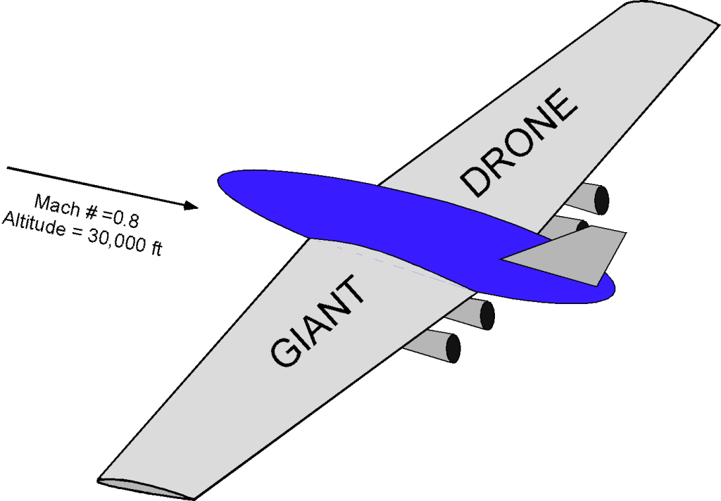
Explain the balance of forces acting on the aircraft.
Calculate the wing’s planform area $S$ and aspect ratio $A\!R$ .
Calculate the aircraft’s airspeed in knots and ft s $^{-1}$ .
Determine the operating lift coefficient $C_L$ of the wing.
Determine the aircraft’s total drag coefficient $C_D$ at its current flight condition.
What is the zero-lift drag coefficient $C_{D_{0}}$ at these flight conditions?
Determine the induced drag coefficient $C_{D_{i}}$ at these flight conditions.
Calculate Oswald’s efficiency factor $e$ for this wing.
Calculate the total drag force acting on the aircraft $D$ and its lift-to-drag ratio $L/D$ .
If the TSFC of each of the four jet engines is 0.5 lb lb $^{-1}$ hr $^{-1}$ , approximately how much fuel will the aircraft burn in 30 minutes of flying time?

1. The aircraft is in equilibrium for steady-level flight, i.e., cruise. The sum of the forces in the vertical direction equals zero, and the sum in the longitudinal direction equals zero. This means that for vertical force equilibrium, then

$L = W$

and for horizontal force equilibrium

$T = D$

2. The wing has two trapezoidal panels, so the total wing area is given by

$S = b \left( \frac{ c_{r} + c_{t}}{2} \right) = 235.0 \left( \frac{35+ 12.25}{2} \right) = 5,552.0~\mbox{ft$^2$}$

The corresponding aspect ratio of the wing is

$A\!R = \frac{b^2}{S} = \frac{235.0^2}{5,552} = 9.95$

3. The airspeed is

$V_{\infty} = M_{\infty} \, a_{\infty} = M_{\infty} \, \sqrt{\gamma R \, T_{\infty}}$

and putting in the numbers gives

$V_{\infty} = 0.80 \sqrt{1.4 \times 1716.49 \times (459.67 + (-47.83)) } = 795.89~\mbox{ft/s}$

Because 1 kt (nautical miles per hour) = 1.688 ft/s, then

$V_{\infty} = 471.5~\mbox{kts}$

4. The aircraft is cruising in steady, straight, and level flight, so $L = W$ and the operating lift coefficient is

$C_{L} = \frac{2W}{\varrho V_{\infty}^{2} S} = \frac{2 \times 684,000}{0.0008903 \times 795.89^2 \times 5,552} = 0.437$

5. The drag polar is given in the question as
C_D = 0.025 + 0.040 \, C_{L}^{2} = C_{D_{0}} + K \, C_{L}^{2} = C_{D_{0}} + C_{D_{i}}
\]
so $C_{D_{0}}$ = 0.025. Substituting $C_{L} = 0.437$ gives for the total drag coefficient

$C_D = 0.025 + 0.040 \times 0.437^{2} = 0.0326$

6. The total drag coefficient $C_{D}$ can be decomposed as

$C_{D} = C_{D_{0}} + C_{D_{i}}$

Therefore, the minimum (non-lifting) drag coefficient is

$C_{D_{0}} = 0.025$

7. The induced (lifting) drag coefficient is

$C_{D_{i}} = K \, C_{L}^{2}= 0.040 \times 0.437^2 = 0.007639$

8. The induced drag coefficient is also given by

$C_{D_{i}} = K \, C_{L}^{2} = \left( \frac{1}{\pi \, AR \, e} \right) C_{L}^{2}$

so solving for Oswald’s efficiency factor gives

$e = \frac{1}{\pi \, K \, A\!R}$

and using the given numerical values gives

$e = \frac{1}{\pi \times 0.040 \times 9.95} = 0.80$

9. The total drag is then

$D = \frac{1}{2}\varrho \, V_{\infty}^{2} \, S \, C_{D}$

and putting in the numbers gives

$D = 0.5 \times 0.0008903 \times 795.89^{2}\times 5, 552 \times 0.0326 = 51,036.3~\mbox{lb}$

So, the lift-to-drag ratio is

$\frac{L}{D} = \frac{684,000}{51,036} = 13.4$

10. The fuel flow rate is

$\overbigdot{W}_{\!f} = ({\rm TSFC}) \, T$

where $T = D$ . Inserting the numbers gives

$\overbigdot{W}_{\!f} = 0.50 \times 51,036 = 25,518~\mbox{lb hr$^{-1}$}$

So, during 30 minutes of flight, the approximate weight of fuel burned is

$W_{f} = \overbigdot{W}_{\!f} \, t = 25,518 \times 0.5 = 12,759~\mbox{lb}$

Worked Example #18

From wind tunnel testing, a new jet airplane has been estimated to have a maximum wing lift coefficient of 3.2 with the slats deployed and the flaps fully down. If the wing loading is 76.84 lb ft^-2, estimate the stalling airspeed in level unaccelerated flight at a pressure altitude of 5,000 ft on a standard ISA day.

The stall airspeed can be estimated using

(1) $\begin{equation*} V_{\rm stall} = \sqrt{ \frac{2}{\varrho_0 \, \sigma } \left( \frac{W}{S} \right) \frac{1}{C_{L_{\rm max}} }} \end{equation*}$

We are told that $C_{L_{\rm max}}$ = 3.2 and that $W/S$ = 76.84 lb ft $^{-2}$ . We can use the ISA model at 5,000 ft on a standard day to determine that $\varrho$ = 0.002048 slugs ft ${^{-3}}$ . Substituting gives

(2) $\begin{equation*} V_{\rm stall} = \sqrt{ \frac{2 \times 76.84}{0.002048} \left( \frac{1}{3.2} \right) } = 153.1~\mbox{ft/s} = 90.7~\mbox{kts} \end{equation*}$

which is relatively low and shows the importance of getting a high value of $C_{L_{\rm max}}$ on a wing.

License

Icon for the Creative Commons Attribution-NonCommercial-NoDerivatives 4.0 International License

Introduction to Aerospace Flight Vehicles Copyright © 2022–2025 by J. Gordon Leishman is licensed under a Creative Commons Attribution-NonCommercial-NoDerivatives 4.0 International License, except where otherwise noted.

Digital Object Identifier (DOI)

https://doi.org/https://doi.org/10.15394/eaglepub.2022.1066.9