Fluid Statics & the Hydrostatic Equation

J. Gordon Leishman

doi:https://doi.org/10.15394/eaglepub.2022.1066.9

12 Fluid Statics & the Hydrostatic Equation

Introduction

In fluid mechanics, a primary concern is describing and understanding the motion or dynamics of the fluid, i.e., the field of fluid dynamics. First, remember that air is just one type of fluid, for which there are many other types in the form of gases and liquids. However, suppose the fluid is not moving or stationary, commonly called a stagnant fluid. In that case, its characteristics and properties (e.g., its pressure, density, etc.) can be described more easily using the physical principles of fluid statics.

A fluid in static equilibrium can be defined as a state where every fluid particle is either at rest or has no relative motion with respect to the other particles in the fluid. No viscous forces act on stagnant fluids because there is no relative motion between the fluid elements. Under these conditions, two types of forces on the fluid must be considered:

Body forces, e.g., weight and inertial accelerations^[1], and possibly electromagnetic forces.^[2]
Surface forces, e.g., the effects of an external pressure acting over an area.

The term hydrostatics is often used to refer to the field of fluid statics in general. Therefore, hydrostatic principles apply to all fluids, both gases and liquids. However, hydrostatics are frequently used to analyze liquids and other predominantly incompressible fluids, i.e., fluids that can be assumed to have constant density. The term aerostatics or pneumatics is used when the principles of fluid statics are applied to gases such as air, which are compressible fluids. Examples of engineering problems that could be analyzed by using hydrostatics and aerostatics include the following:

The measurement of pressure using various types of manometry.
The buoyancy and stability of floating objects, such as ships in the water, and lighter-than-air aircraft, such as balloons and blimps.
The pressure and other fluid properties inside containers or vessels, including under the action of body forces or acceleration fields.
The properties of the atmosphere on Earth and other planets.
The transmission of forces and power using pressurized liquids and/or gases.

Learning Objectives

Understand the meaning of a stagnant fluid and the underlying principles that apply to the behavior of static fluids.
Derive, understand, and use the general equations for an aero-hydrostatic pressure field.
Understand how to develop and apply the aero-hydrostatic equation.
Use the principles of hydrostatics and the aero-hydrostatic equation to solve some fundamental engineering problems.

Pascal’s Law

The pressure at a point in a fluid at rest is equal in all directions, so the pressure is an isotropic scalar quantity formally embodied in Pascal’s Law. The derivation of Pascal’s Law proceeds by considering an infinitesimally small right-angled, three-dimensional fluid wedge at rest. However, the outcome is most easily obtained if the wedge is examined in just one view (or one plane), as shown in the figure below, which appears as a right-angled triangle with horizontal side length $dx$ , vertical side length $dy$ , and diagonal length $ds$ , with the contained angle $\theta$ .

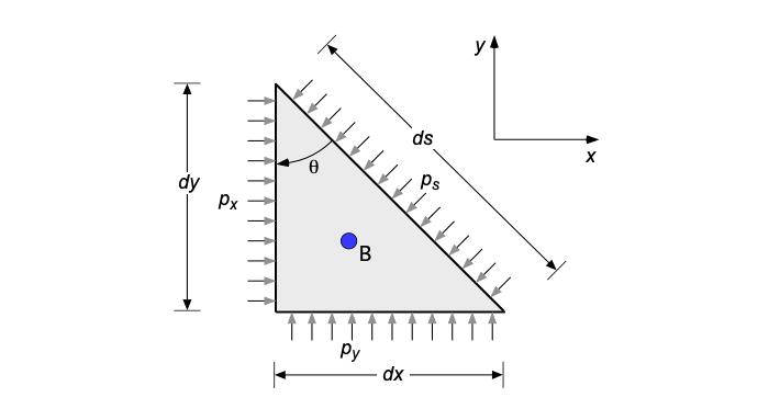
The pressures acting on the respective faces are $p_{x}$ in the $x$ -direction, $p_{y}$ in the $y$ -direction, and $p_{s}$ along the diagonal. Therefore, for horizontal pressure force equilibrium on the fluid per unit length (1 unit into the page), then

(1) $\begin{equation*} p_x \, (1) \, dy - p_s \, (1) \, ds \cos \theta = 0 \end{equation*}$

For the vertical pressure force equilibrium per unit length, then

(2) $\begin{equation*} p_y \, (1) \, dx - p_s \, (1) \, ds \sin \theta - dW = 0 \end{equation*}$

where $dW$ is the weight of the fluid per unit length, i.e.,

(3) $\begin{equation*} dW = \varrho g \, \left( \frac{dx \, dy}{2} \right) \, (1) \end{equation*}$

From the geometry of the triangle in the figure, then $dx = ds \sin \theta$ and $dy = ds \cos \theta$ . Also, as the triangle shrinks to point B in the fluid, but such that $dx$ and $dy$ become of $\mathcal{O} (\delta)$ in accordance with the continuum assumption, then the product $dx \, dy$ becomes negligible, i.e., the effects of the weight of fluid inside can be neglected. So, it becomes apparent that

(4) $\begin{equation*} p_y \, dx - p_s \, dx = 0 \end{equation*}$

and

(5) $\begin{equation*} p_x \, dy - p_s \, dy = 0 \end{equation*}$

Therefore, from these two latter equations, the conclusion reached is that as the triangle shrinks to the point B, then

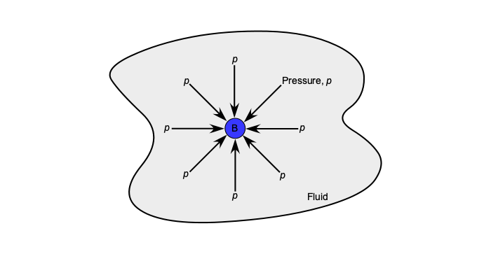
(6) $\begin{equation*} p_x = p_y = p_s = \mbox{~constant} = p \end{equation*}$

which states that the pressure at any point in a fluid at rest is the same in all directions, as shown in the figure below; this is called Pascal’s Law. This latter derivation is easily generalized to three dimensions to show that $p_x = p_y = p_z = \mbox{constant} = p$ .

Pascal’s Law states that the pressure at a point is constant and acts equally in all directions.

Aerostatic/Hydrostatic Pressure Field

Remember that pressure is a point property and can have a different value from one part to another in the fluid. With the concept of pressure already discussed, the formal derivation of the equations for the pressure variation in a stagnant fluid can now proceed, and with a particular case of these equations, called the aero-hydrostatic equation. Consider in the differential sense an infinitesimally small volume of fluid in a stagnant flow, i.e., a fluid element of volume $dx \, dy \, dz = d {\cal{V}}$ , as shown in the figure below. As the volume becomes infinitesimally small in the limit, it shrinks to point B such that $d {\mathcal{V}} \rightarrow \mathcal{O} (\delta^3)$ in accordance with the continuum assumption.

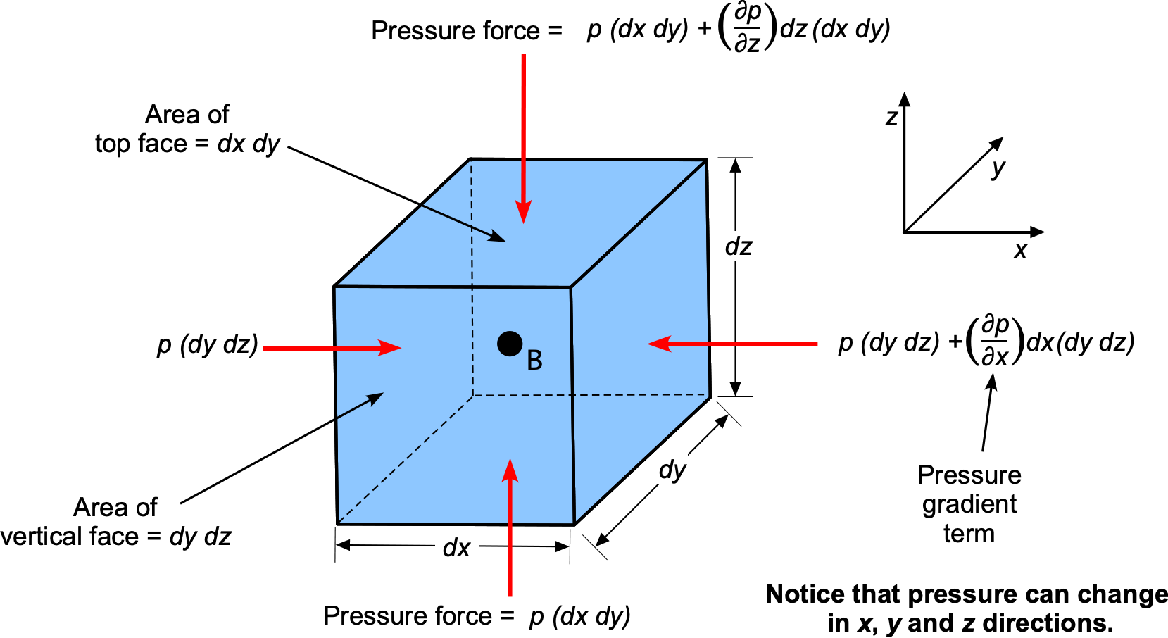
Pressure forces acting on an infinitesimally small, stationary fluid volume with pressure gradients in three directions.

Acting on this small fluid volume are:

Pressure forces from the surrounding fluid act normal to the surfaces and vary from point to point, i.e., $p = p(x, y, z)$ .
Body forces, in general, which are usually expressed as per unit mass of fluid, i.e., $\vec{f}_{b} = f_x \, \vec{i} + f_y \, \vec{j} + f_z \, \vec{k}$ per unit mass, where the mass in this case is $dm = \varrho (dx \, dy \, dz) = \varrho \, d {\mathcal{V}}$ .
A specific body force in the form of gravity, which manifests as a vertically downward force from the weight of fluid inside the element. This gravitational force can be written as $\vec{f}_{b} = -g \, \vec{k}$ per unit mass of fluid, i.e., the negative sign indicating that the force of gravity acts downward.

Units of body force per unit mass

Notice the units of a body force per unit mass has dimensions of acceleration, i.e., force per unit mass = force/mass = acceleration, so it has units of length/time². Therefore, body forces can also arise from any inertial accelerations of the fluid, e.g., while there is no relative motion between the fluid particles, the entire fluid mass can be subjected to accelerations. While fluid forces from electromagnetic or electrostatic effects are not a consideration for air, certain types of fluids have properties that respond to such fields and may be explicitly selected for that purpose.

Consider the pressure forces in the $x$ direction, i.e., on the $y$ – $z$ face of area $dy \, dz$ . Let $\dfrac{\partial p}{\partial x}$ be the change of pressure $p$ with respect to $x$ . Notice that the partial derivative must be used because the pressure could vary in all three spatial directions. The net pressure force in the $x$ direction is

(7) $\begin{equation*} d F_x = p \left( dy \, dz \right) - \left( p + \frac{\partial p}{\partial x} dx \right) dy \, dz = -\frac{\partial p}{\partial x} \left(dx \, dy \, dz \right) \end{equation*}$

Similarly, for the $y$ direction, the net pressure force is

(8) $\begin{equation*} d F_y = p \left( dx \, dz \right) - \left( p + \frac{\partial p}{\partial y} dy \right) dx \, dz = -\frac{\partial p}{\partial y} \left(dx \, dy \, dz \right) \end{equation*}$

and in the $z$ direction, the net pressure force is

(9) $\begin{equation*} d F_z = p \left( dx \, dy \right) - \left( p + \frac{\partial p}{\partial z} dz \right) dx \, dy = -\frac{\partial p}{\partial z} \left(dx \, dy \, dz \right) \end{equation*}$

Therefore, the net resultant pressure force on the fluid element is

(10) $\begin{eqnarray*} d\vec{F} & = & dF_x \, \vec{i} + dF_y \, \vec{j} + dF_z \, \vec{k} \\[6pt] & = & -\left( \frac{\partial p}{\partial x} \, \vec{i} + \frac{\partial p}{\partial y} \, \vec{j} + \frac{\partial p}{\partial z} \, \vec{k} \right) dx \, dy \, dz \nonumber \\[6pt] & = & -\nabla p \, (dx \, dy \, dz ) = -\nabla p \, d {\mathcal{V}} \end{eqnarray*}$

where the gradient vector operator $\nabla$ (i.e., “del” or “grad”) has now been introduced.

If $\varrho$ is the mean density of the fluid element, then the total mass of the fluid element, $dm$ , is $\varrho \left(dx \, dy \, dz \right) = \varrho \, d {\mathcal{V}}$ , as shown in the figure below. Any coordinate system can be assumed, but usually, $z$ is defined as positive in the vertical direction, where the gravitational acceleration would be $-g\, \vec{k}$ . As such, gravity manifests as a vertically downward force from the weight of fluid inside the element, i.e., the net gravitational force is $-\varrho \, d {\mathcal{V}} \, g \, \vec{k}$ .

Body forces per unit mass acting on a fluid can include inertial accelerations and acceleration under gravity, i.e., weight.

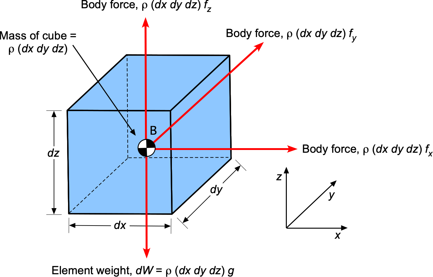
Furthermore, any additional body forces per unit mass acting on the element can be described as

(11) $\begin{equation*} \vec{f}_{b} = f_x \, \vec{i} + f_y \, \vec{j} + f_z \, \vec{k} \end{equation*}$

Now, if a fluid element is at rest and in equilibrium, then the sum of the pressure forces, the gravitational force, and the body force must be zero, i.e.,

(12) $\begin{equation*} -\nabla p \, d {\mathcal{V}} + \varrho \, d {\mathcal{V}} \vec{f}_{b} - \varrho \, d {\mathcal{V}} \, g\, \vec{k} = 0 \end{equation*}$

or

(13) $\begin{equation*} \nabla p = \varrho \, \vec{f}_{b} -\varrho \, g\, \vec{k} \end{equation*}$

In scalar form, the preceding vector equation can be written as

(14) $\begin{eqnarray*} \frac{\partial p}{\partial x} & = & \varrho \, f_x \nonumber \\[6pt] \frac{\partial p}{\partial y} & = & \varrho \, f_y \nonumber \\[6pt] \frac{\partial p}{\partial z} & = & \varrho \, f_z -\varrho \, g \nonumber \end{eqnarray*}$

Therefore, these three partial differential equations describe the pressure variations within a stagnant fluid. Notice that the center of gravity is at the centroid of the fluid element, so no gravitational moments are acting on the element.

Effects of Gravity Alone

If the only body force is the effects of gravitational acceleration or gravity force (the weight) acting on the element, then

(15) $\begin{equation*} d\vec{W} = -\varrho \, d {\mathcal{V}} \, g \, \vec{k} \end{equation*}$

where $g$ is acceleration under gravity. Gravity manifests as a downward force, so there is a minus sign in the $z$ direction, i.e., it is downward because $z$ is measured positively upward. Therefore, in this case

(16) $\begin{equation*} \nabla p = -\varrho \, g \, \vec{k} \end{equation*}$

or in scalar form

(17) $\begin{eqnarray*} \frac{\partial p}{\partial x} & = & 0 \nonumber \\[6pt] \frac{\partial p}{\partial y} & = & 0 \nonumber \\[6pt] \frac{\partial p}{\partial z} & = & -\varrho \, g \nonumber \\ \end{eqnarray*}$

Because the pressure does not depend on $x$ or $y$ , the above equation can now be written as
the ordinary differential equation

(18) $\begin{equation*} \frac{dp}{dz} = -\varrho \, g \end{equation*}$

This differential equation is called the hydrostatic equation or sometimes the aero-hydrostatic equation. The aero-hydrostatic equation relates the change in pressure $dp$ in a fluid to a change in vertical height $dz$ . Equation 18 has many uses in manometry, hydrodynamics, and atmospheric physics, including the derivation of the properties of the International Standard Atmosphere (ISA), which is considered later.

Solutions to the Aero-Hydrostatic Equation

Several special cases of interest lead to helpful solutions to the aero-hydrostatic equation, namely the pressure changes for:

A constant density fluid, i.e., a liquid.
A constant temperature gas.
A linear temperature gradient in a gas.

In the case of gases, once the pressure is known, the corresponding density and/or temperature of the gas can also be solved using the equation of state, i.e.,

(19) $\begin{equation*} p = \varrho \, R \, T \end{equation*}$

Remember that the equation of state can be used to relate the pressure, $p$ , density, $\varrho$ , and temperature, $T$ , of a gas. If one of these quantities is unknown, then the values of two others can be used to determine the unknown quantity. In the case of liquids, there is no equivalent equation of state because it is incompressible, and the density is constant.

Isodensity Fluid

If a fluid’s density is assumed to be a constant, e.g., a liquid, then Eq. 18 can be easily integrated from one height to another to find the corresponding change in pressure. Separating the variables gives

(20) $\begin{equation*} \int_{p_1}^{p_2} dp = -\varrho \, g \int_{z_1}^{z_2} dz \end{equation*}$

and so

(21) $\begin{equation*} p_2 - p_1 = -\varrho \, g \left( z_2 - z_1 \right) \end{equation*}$

or

(22) $\begin{equation*} \Delta p = -\varrho \, \Delta z \end{equation*}$

This result also means that

(23) $\begin{equation*} p_1 + \varrho \, g \, z_1 = p_2 + \varrho \, g \, z_2 \end{equation*}$

or perhaps in a more familiar form, as

(24) $\begin{equation*} p + \varrho \, g \, z = \mbox{constant} \end{equation*}$

where $z$ is “height.” This simple equation has many uses in various forms of manometry, but its use is restricted to incompressible fluids, i.e., liquids.

Isothermal Gas

If the temperature of a gas is assumed to be constant, i.e., what is known as an isothermal condition, then $T= T_0 =$ constant. In this case, then

(25) $\begin{eqnarray*} \frac{dp}{dz} & = & -\varrho \, g \\[8pt] T & = & T_0 \\[8pt] p & = & \varrho \, R \, T \end{eqnarray*}$

By substituting for $\varrho$ and assuming isothermal conditions, then

(26) $\begin{equation*} \frac{dp}{p}= - \frac{g}{R \, T_0} dz \end{equation*}$

Integrating from $z_1$ to $z_2$ where the pressures are $p_1$ and $p_2$ , respectively, gives

(27) $\begin{equation*} \int_{p_1}^{p_2} \frac{dp}{p}= -\frac{g}{R \, T_0} \int_{z_1}^{z_2} dz \end{equation*}$

and performing the integration gives

(28) $\begin{equation*} \ln p_2 - \ln p_1= \ln \left( \frac{p_2}{p_1} \right) = -\frac{g}{R \, T_0} \left( z_2 - z_1 \right) \end{equation*}$

Therefore,

(29) $\begin{equation*} \frac{p_2}{p_1} = \exp \left( -\frac{g (z_2 - z_1)}{R \, T_0} \right) \end{equation*}$

Notice also that for isothermal conditions

(30) $\begin{equation*} \frac{\varrho_2}{\varrho_1} = \frac{p_2}{p_1} \end{equation*}$

Linear Temperature Gradient in a Gas

If the temperature of a gas decreases linearly with height, i.e., $T = T_0 - \alpha \, z$ where $\alpha$ is the thermal gradient or “lapse rate,” then in this case

(31) $\begin{eqnarray*} \frac{dp}{dz} & = & -\varrho \, g \\[6pt] T & = & T_0 - \alpha \, z \\[6pt] p & = & \varrho \, R \, T \end{eqnarray*}$

Substituting the other two equations into the differential equation gives

(32) $\begin{equation*} \frac{dp}{dz} = -\varrho \, g = - \left( \frac{p}{R \, T} \right) g = -\frac{p \, g}{R (T_0 - \alpha \, z)} \end{equation*}$

which is the governing equation that now needs to be solved. By means of separation of variables and integrating from $z_1$ to $z_2$ where the pressures are $p_1$ and $p_2$ , respectively, gives

(33) $\begin{equation*} \int_{p_1}^{p_2} \frac{dp}{p} = - \frac{g}{R} \int_{z_1}^{z_2}\frac{dz}{T_0 - \alpha \, z} \end{equation*}$

Performing the integration gives for the left-hand side

(34) $\begin{equation*} \int_{p_1}^{p_2} \frac{1}{p} \, dp = \ln\left(\frac{|p_2|}{|p_1|}\right) \end{equation*}$

and for the right-hand side

(35) $\begin{equation*} \int_{z_1}^{z_2} \frac{1}{T_0 - \alpha \, z} \, dz = -\frac{1}{\alpha} \ln\left(\frac{|T_0 - \alpha \, z_2|}{|T_0 - \alpha \, z_1|}\right) \end{equation*}$

and so the final solution is

(36) $\begin{equation*} \frac{p_2}{p_1} = \left|\frac{T_0 - \alpha \, z_2}{T_0 - \alpha \, z_1}\right|^{\left( \displaystyle{\frac{g}{R \, \alpha}}\right)} \end{equation*}$

The corresponding density ratio is

(37) $\begin{equation*} \frac{\varrho_2}{\varrho_1} = \left|\frac{T_0 - \alpha \, z_2}{T_0 - \alpha \, z_1}\right|^{\left( \displaystyle{\frac{g}{R \, \alpha} - 1}\right) } \end{equation*}$

Hydrostatic Paradox

Consider the situation in the figure below, which shows three different-shaped containers filled with the same liquid. What are the pressure values on the container’s bottom in each case? The answer is that the pressures are all the same because the hydrostatic equation shows the pressure at a point in a liquid depends only upon the height of the other liquid directly above it, $H$ , and not at all upon the container’s shape.

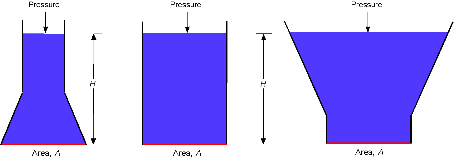
According to the principles of hydrostatics, the pressure on the bottom of each container is the same, regardless of its shape and the volume (or weight) of liquid above it.

The pressure at the bottom of each container is $p =\varrho \, g \, H$ , where $\varrho$ is the density of the liquid. If each container has the same area $A$ at the bottom, then the pressure force, $F = p A$ on each container’s base, is the same. This outcome is independent of the volume of liquid, and the weight of the liquid in each container is different and is referred to as the hydrostatic paradox.

Check Your Understanding #1 – Pressure on the bottom of a container

Consider a cylindrical tank containing two liquids of density $\varrho_1$ and $\varrho_2$ , as shown in the figure below. Determine an expression for the pressure on the bottom of the tank, $p_A$ . If the heights are $h_1 = 12.1$ cm and $h_2 = 13.4$ cm, and the densities are $\varrho_1 = 970$ kg/m ${^3}$ and $\varrho_2 = 1,100$ kg/m ${^3}$ . Assume standard atmospheric pressure, $p_{\rm atm} = 101.325$ kPa. If the liquids are mixed to form a homogeneous fluid of density $\varrho_{\rm mix}$ , what will be the pressure on the bottom of the tank?

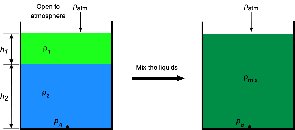
Show solution/hide solution.

For the unmixed liquids, the static pressure on the bottom of the tank will be

$p_A = p_{\rm atm} + \varrho_1 \, g \, h_1 + \varrho_2 \, g \, h_2$

Inserting the values gives

$p_A = 101.325 \times 10^3 + 970.0 \times 9.81 \times 0.121 + 1,100 \times 9.81 \times 0.134 = 103.791\mbox{kPa}$

If the two liquids are homogeneously mixed, then

$p_B = p_{\rm atm} + \varrho_{\rm mix} \, g \left( h_1 + h_2 \right)$

The mixing will not change the net mass of the two liquids, so by conservation of mass, then

$M = \left( \varrho_1 \, g \, h_1 + \varrho_2 \, g \, h_2 \right) A = \varrho_{\rm mix} \, g \left( h_1 + h_2 \right) A$

where $A$ is the cross-sectional area of the tank. Therefore,

$\varrho_{\rm mix} \, g \, \left( h_1 + h_2 \right) = \left( \varrho_1 \, g \, h_1 + \varrho_2 \, g \, h_2 \right)$

Substituting into the expression for $p_B$ gives

$p_B = p_{\rm atm} + \varrho_{\rm mix} \, g \left( h_1 + h_2 \right) = p_{\rm atm} + \left( \varrho_1 \, g \, h_1 + \varrho_2 \, g \, h_2 \right) = p_A$

Therefore, the pressure on the bottom of the container is not changed by mixing the two liquids.

Archimedes’ Principle

Archimedes’ principle (also spelled Archimedes’s principle) is commonly used to solve problems in hydrostatics^[3]. This principle states that the upward or buoyancy force exerted on a body immersed in a fluid equals the weight of the fluid that the body displaces. This outcome occurs whether the body is wholly or partially submerged in the fluid and is independent of the body’s shape. The resulting force also acts upward at the center of buoyancy (the center of mass) of the displaced fluid. This principle is commonly used in problems involving floatation or “floating bodies,” such as boats, ships, balloons, and airships. Balloons and airships are known as aerostats or lighter-than-air (LTA) aircraft in aviation.

Derivation of Archimedes’ Principle

Having introduced the concept of hydrostatic pressure and the hydrostatic equation, the derivation of Archimedes’ principle is now relatively straightforward because it will be apparent that the source of buoyancy is a consequence of a pressure difference acting on the body. To this end, consider a solid body wholly immersed in a fluid of constant density, as shown in the figure below. The elemental volume, $d{\cal{V}}$ has linear dimensions of $dx$ , $dy$ , and $dz$ .

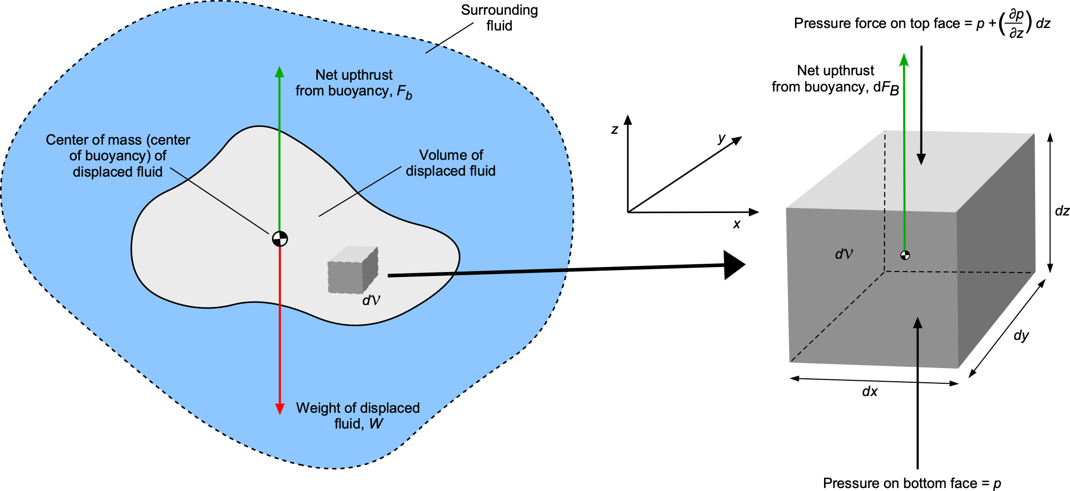
The hydrostatic pressure force on the top face of the volume $d{\cal{V}}$ will be lower than that on the bottom face, the difference being the source of the upthrust (buoyancy) on the body. It will be apparent that there are no net forces on $d{\cal{V}}$ in the $x$ and $y$ directions. The net pressure force in the upward $z$ direction, which is the elemental buoyancy force, $dF_B$ , will be

(38) $\begin{equation*} dF_B = p \, dx \, dy - \left( p + \dfrac{\partial p}{\partial z} \, dz \right) dx \, dy = -\dfrac{\partial p}{\partial z} \, dx \, dy \, dz = -\dfrac{\partial p}{\partial z} \, d {\cal{V}} \end{equation*}$

Using the hydrostatic equation gives

(39) $\begin{equation*} \frac{\partial p}{\partial z} = \frac{dp}{dz} = -\varrho\, g \end{equation*}$

Therefore, the buoyancy force on $d {\cal{V}}$ is

(40) $\begin{equation*} dF_B = -\dfrac{d p}{d z} \, d {\cal{V}} = - (-\varrho \, g) d {\cal{V}} = \varrho \, g \, d{\cal{V}} \end{equation*}$

Therefore, the total buoyancy force on the immersed body is

(41) $\begin{equation*} F_B = \oiiint_{\cal{V}} \varrho \, g \, d{\cal{V}} = \varrho \, g \oiiint_{\cal{V}} \, d{\cal{V}} \end{equation*}$

Because the shape of the body is arbitrary, then

(42) $\begin{equation*} F_B = \varrho \, g \oiiint_{\cal{V}} \, d{\cal{V}} = \varrho \, g \, {\cal{V}} \end{equation*}$

which is the net weight of the fluid of density $\varrho$ displaced by the volume ${\cal{V}}$ of the immersed body.

Therefore, the derivation concludes by stating that the upthrust on the immersed body is equal to the weight of the fluid displaced by the body, i.e., Archimedes’ principle, which is a consequence of the net difference in hydrostatic pressure force acting on the body. This latter result applies to an immersed body of any shape, including one partially submerged in a fluid.

Check Your Understanding #2 – Buoyancy force

Which balloon shown in the figure below experiences the most significant buoyancy force? Each balloon contains the same volume of fluid and is surrounded by air.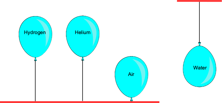

Show solution/hide solution.

The answer is all balloons experience the same buoyancy force because they all displace the same volume of air. An assumption is that the water balloon does not stretch with the weight of water. According to Archimedes’ principle, the buoyancy force is equal to the weight of the fluid displaced, not the weight of the fluid inside the balloon. The net upforce, however, does depend on the fluid inside the balloon, in which case the balloon with the lightest gas (hydrogen) will be the largest. Note: This was not meant to be a trick question.

Buoyancy & Floatation

To better illustrate the concept of buoyancy, consider the scenarios shown in the figure below. The object’s volume is the same in each case, but its weight differs, ranging from $W_1$ (the heaviest) to $W_4$ (the lightest). If the object is entirely immersed in the fluid, then the upthrust of buoyancy force, $F_b$ , will be

(43) $\begin{equation*} F_b = \varrho_{\rm fluid} \, {\cal{V}} \, g \end{equation*}$

where ${\cal{V}}$ is the volume of the object and hence the displaced fluid, and $\varrho_{\rm fluid}$ is the density of the displaced fluid. Remember that the buoyancy force depends on the weight of the fluid displaced by the object, not the weight of the object itself.

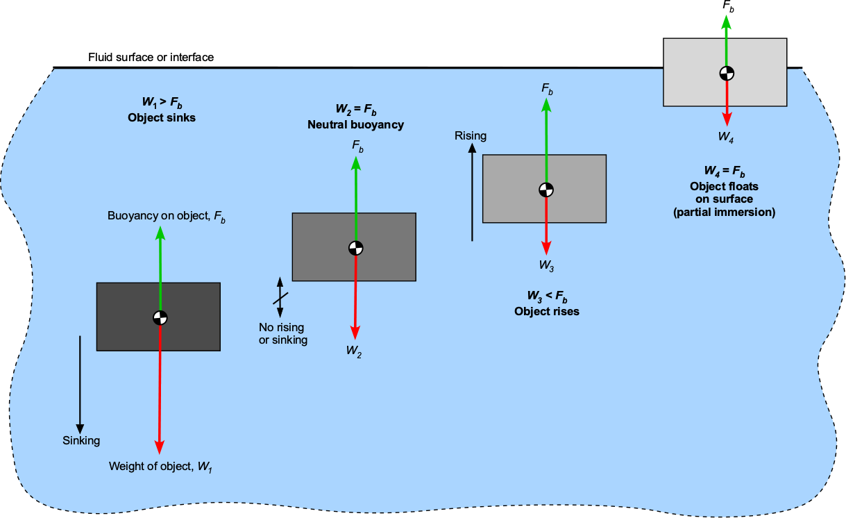
The principle of buoyancy and floatation can be better understood by considering what happens to an immersed object of fixed volume but of different weights.

The net force on the body, therefore, is

(44) $\begin{equation*} F_u = F_b - W \end{equation*}$

It will begin to sink if the object is heavier than the buoyancy force, i.e., $F_u < 0$ . If the object has a weight equal to the buoyancy force, i.e., $F_u = 0$ , it will have neutral buoyancy and reach an immersed depth where it will neither sink nor rise in the fluid, i.e., neutral buoyancy like a submarine. The body will begin to rise in the fluid if the buoyancy force exceeds the weight, i.e, $F_u > 0$ . Eventually, if the body is made light enough, it will float on the surface of the fluid interface. In this case, only partial immersion may be needed to displace the fluid required to create the buoyancy force to balance its weight, i.e., like a boat or a ship.

As shown in the figure below, consider an LTA aircraft floating in the air. The gas envelope is filled with some volume of another (lighter) gas, called the buoyant gas. In the case of the airship, the gas inside will be helium, which is eight times lighter than air. In the case of the balloon, the gas is hot air, which has only a moderately lower density than the surrounding cooler air, depending on its temperature. In either case, the upthrust or buoyancy lift force will equal the weight of displaced air. Often, this upforce is called an aerostatic lift because it does not depend on the motion.

The net force acting on an LTA aircraft is equal to the difference between the downward-acting weight of the vehicle and the upward buoyancy force, which is equal to the weight of the displaced air.

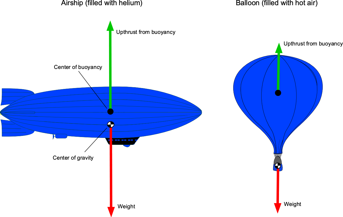
The LTA aircraft’s net weight will include the weight of its structure, payload, fuel, etc., plus the weight of gas contained within the gas envelope. Therefore, the net force acting will equal the difference between the net weight of the vehicle minus the weight of the displaced air (i.e., the buoyancy or “upthrust”). If the upthrust is greater than the weight, the aircraft will rise; if it is less, it will descend. Equilibrium, or neutral buoyancy, will be achieved when these two forces are equal and are in exact vertical balance.

These aerostatic principles can be further developed by using Archimedes’ principle. The net upforce (aerostatic lift), $L$ , will be equal to the net weight of the air displaced less the weight of the gas inside the envelope, i.e., the aerostatic lift is

(45) $\begin{equation*} L = \left( \varrho_{\rm air} - \varrho_{\rm gas} \right) g \,{\cal{V}} \end{equation*}$

where ${\cal{V}}$ is the volume of the envelope containing the buoyant gas, $\varrho_{\rm gas}$ is the density of the buoyant gas, and $\varrho_{\rm air}$ is the density of the displaced air. If the weight of the aircraft is $W$ , then for vertical force equilibrium and neutral buoyancy, then

(46) $\begin{equation*} L = W = \left( \varrho_{\rm air} - \varrho_{\rm He} \right) g \, {\cal{V}} \end{equation*}$

Therefore, the volume of the buoyant gas can be determined to give a specific buoyancy force to overcome the weight. This is the fundamental principle of aerostatic lift production on all types of LTA aircraft.

Check Your Understanding #3 – Buoyancy of an airship

An airship has an aerostatic gas envelope with a 296,520 ft³ volumetric capacity; helium is used. If the airship has an empty weight of 14,188 lb and a maximum fuel load of 960 lb, what would be the maximum payload the airship could carry? Assume MSL ISA standard atmospheric conditions. The density of helium can be assumed to be 0.0003192 slugs/ft³. Ignore the effects of any ballast.

Show solution/hide solution.

The hydrostatic principle of buoyancy is applicable here. Using Archimedes’ principle, the upforce (aerostatic lift), $L$ , on the airship will be equal to the net weight of the fluid displaced minus the weight of the gas inside the envelope, i.e.,

$L = \left( \varrho_{\rm air} - \varrho_{\rm He} \right) g \, {\cal{V}}$

where ${\cal{V}}$ is the volume of the gas envelope. The gross weight of the airship will be the sum of the empty weight, $W_e$ , plus the fuel weight, $W_f$ , plus the payload, $W_p$ , i.e.,

$W = W_e + W_f + W_p$

For vertical force equilibrium at takeoff with neutral buoyancy, then $L = W$ , so

$W_e + W_f + W_p = \left( \varrho_{\rm air} - \varrho_{\rm He} \right) g {\, \cal{V}}$

Rearranging to solve for the payload weight gives

$W_p = \left( \varrho_{\rm air} - \varrho_{\rm He} \right) g \, {\cal{V}} - W_e - W_f$

Using the numerical values supplied gives

$W_p = \left( 0.002378 - 0.0003192 \right) \times 32.17 \times 296,520 - 14,188.0 - 960.0 = 4,497.45~\mbox{lb}$

Therefore, the maximum payload at the takeoff point would be 4,497 lb.

Horizontal Buoyancy Effects

Horizontal buoyancy effects can be produced when buoyancy forces act in directions other than vertically, which can arise from horizontal gradients in fluid density, pressure, or temperature. These effects can be significant in various scientific and engineering applications. Recall that the horizontal buoyancy force on an elemental volume $d{\cal{V}}$ from a pressure gradient in the $x$ direction is given by

(47) $\begin{equation*} F_{B_{x}} = - \left( \frac{\partial p}{\partial x} \right) d{\cal{V}} \end{equation*}$

and the corresponding force in the $y$ direction by

(48) $\begin{equation*} F_{B_{y}} = - \left( \frac{\partial p}{\partial y} \right) d{\cal{V}} \end{equation*}$

Such horizontal buoyancy effects are a consideration in the aerodynamic testing of models in wind tunnels. A longitudinal pressure gradient in the test section can form because of the growth of the boundary layers on the test section walls, resulting in a horizontal buoyancy force that affects the drag measurements. For example, if an axisymmetric body of length $L$ and projected frontal area $A_f$ is assumed, as shown in the figure below, then according to Eq. 47, the horizontal buoyancy drag force increment will be

(49) $\begin{equation*} \Delta D_{B_{x}} = - \left( \frac{\partial p}{\partial x} \right) \oiiint_{\cal{V}} d{\cal{V}} \approx - \left( \frac{\partial p}{\partial x} \right) A_f \, L \end{equation*}$

In most wind tunnels, the pressure gradient is (by design) negligible or slightly negative, so $\Delta D_{B_{x}}$ will be positive.

The creation of a horizontal buoyancy force in a wind tunnel because of a longitudinal pressure gradient in the test section is a source of a “virtual” drag force or drag tare.

While the cross-sectional area of the test section is usually designed to increase slightly in the downstream direction to minimize this longitudinal pressure gradient, a slight residual horizontal buoyancy tare drag may remain, particularly with larger and longer bodies. Therefore, the drag measurements may need to be corrected. For example, this drag tare would be subtracted from the measurements made with a force balance.

Likewise, temperature and density gradients can also affect the measurements, e.g., because of solar heating of the tunnel shell, an issue for most larger tunnels. A temperature-controlled wind tunnel maintains a mixed flow with a constant temperature, ensuring uniform airflow and minimizing horizontal buoyancy effects from thermal sources. But if the flow has a measurable vertical temperature gradient, i.e., $\dfrac{\partial T}{\partial z}$ , then a horizontal buoyancy drag can be produced. The corresponding vertical density gradient will be

(50) $\begin{equation*} \frac{\partial \varrho}{\partial z} = -\frac{\varrho g}{T} - \frac{p}{R T^2} \left( \frac{\partial T}{\partial z} \right) \end{equation*}$

when using the equation of state. With the aid of the hydrostatic equation, then

(51) $\begin{equation*} \varrho = -\frac{1}{g} \left( \frac{\partial p}{\partial z} \right) \end{equation*}$

and substituting gives

(52) $\begin{equation*} \frac{\partial \varrho}{\partial z} = \frac{1}{T} \left( \frac{\partial p}{\partial z} \right) - \frac{p}{R T^2} \left( \frac{\partial T}{\partial z} \right) \end{equation*}$

Therefore, the horizontal pressure gradient in terms of the vertical temperature gradient is

(53) $\begin{equation*} \frac{\partial p}{\partial x} = - g \left( \frac{p}{R T^2} \right) \frac{\partial T}{\partial z} \end{equation*}$

The horizontal buoyancy drag force, in this case from a thermal gradient, is

(54) $\begin{equation*} \Delta D_{B_{x}} = - \left( \frac{\partial p}{\partial x} \right) \, d{\cal{V}} \end{equation*}$

and by substituting for the pressure gradient, then

(55) $\begin{equation*} \Delta D_{B_{x}} = -\left(- g \left(\frac{p}{R T^2} \right) \frac{\partial T}{\partial z}\right) \, d{\cal{V}} \end{equation*}$

and so, finally, then

(56) $\begin{equation*} \Delta D_{B_{x}} = g \left(\frac{p}{R T^2} \right) \, \frac{\partial T}{\partial z} \, d{\cal{V}} \end{equation*}$

or for the axisymmetric body, then

(57) $\begin{equation*} \Delta D_{B_{x}} \approx \left( \frac{g \, p}{R \, T^2}\right) \frac{\partial T}{\partial z} \, A_f \, L \end{equation*}$

In most wind tunnels, such as those exposed on one or more sides to solar radiation, the value of $~\dfrac{\partial T}{\partial z}$ is positive, perhaps reaching several degrees Celcius per meter. While the buoyancy tare effect is generally small, except with large models, the drag values are also small, so even minor effects can have sizable contributions to the uncorrected drag measurements. For the best quality measurements, a temperature-controlled wind tunnel is needed to maintain a mixed flow to ensure uniform airflow and minimize horizontal buoyancy effects from thermal sources.

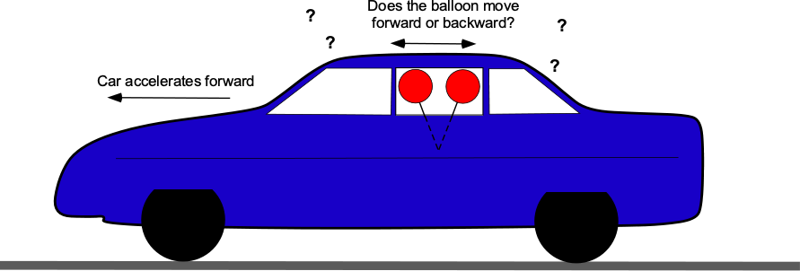
Check Your Understanding #4 – Baffling balloon behavior!

A helium-filled party balloon tied to a string attached to the seat floats inside a car. If the vehicle accelerates forward, in which direction will the balloon move? For a demonstration, use this link: Baffling Balloon Behavior. Can you explain the physics of this behavior using the principles of hydrostatics?

Show solution/hide solution.

The answer is obtained by using Archimedes’ principle. The net up-force from buoyancy, $L$ , on the balloon will be equal to the net weight of the air displaced, less the weight of the helium inside the balloon, as shown in the figure below, i.e.,

$L = \varrho_{\rm air} \, g \, {\cal{V}} - \varrho_{\rm He} \, g \, {\cal{V}} = \left( \varrho_{\rm air} - \varrho_{\rm He} \right) g \, {\cal{V}}$

where ${\cal{V}}$ is the volume of the balloon, $\varrho_{\rm air}$ is the density of air, and $\varrho_{\rm He}$ is the density of the helium gas inside the balloon. We are told to neglect the weight of the balloon itself. Therefore, the tension, $T$ , on the string is

$T = L = \left( \varrho_{\rm air} - \varrho_{\rm He} \right) g \, {\cal{V}}$

If the car moves forward with a constant acceleration, $a$ , in the $x$ direction, then the balance of forces on the balloon will change, as shown in the figure. Because the air mass inside the car is stagnant, the acceleration to the left (positive $x$ direction) manifests as an inertial body force on the stagnant air directed to the right (negative $x$ direction). This acceleration will create a horizontal pressure gradient (the higher pressure biased to the rear of the car) that will lead to a net horizontal buoyancy force directed toward the left, i.e.,

$F_x = \left( \varrho_{\rm air} - \varrho_{\rm He} \right) a \, {\cal{V}}$

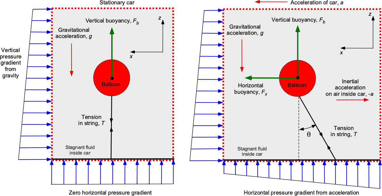In other words, because of the much lighter helium gas in the balloon, the horizontal buoyancy force in the air is greater than its inertial force. Therefore, it can be concluded that the helium balloon will lean forward relative to the car when accelerating forward. Finding the angle of the string for horizontal and vertical force equilibrium is just the application of statics, i.e.,

$T \cos \theta = F_x$

and

$T \sin \theta = L$

Therefore,

$\tan \theta = \frac{F_x}{L} = \frac{ \left( \varrho_{\rm air} - \varrho_{\rm He} \right) a \, {\cal{V}}} {\left( \varrho_{\rm air} - \varrho_{\rm He} \right) \, g {\cal{V}}} = \frac{a}{g}$

So, finally, the angle of the string is

$\theta = \tan^{-1} \left( \frac{a}{g} \right)$

Pressure Forces on Submerged Surfaces

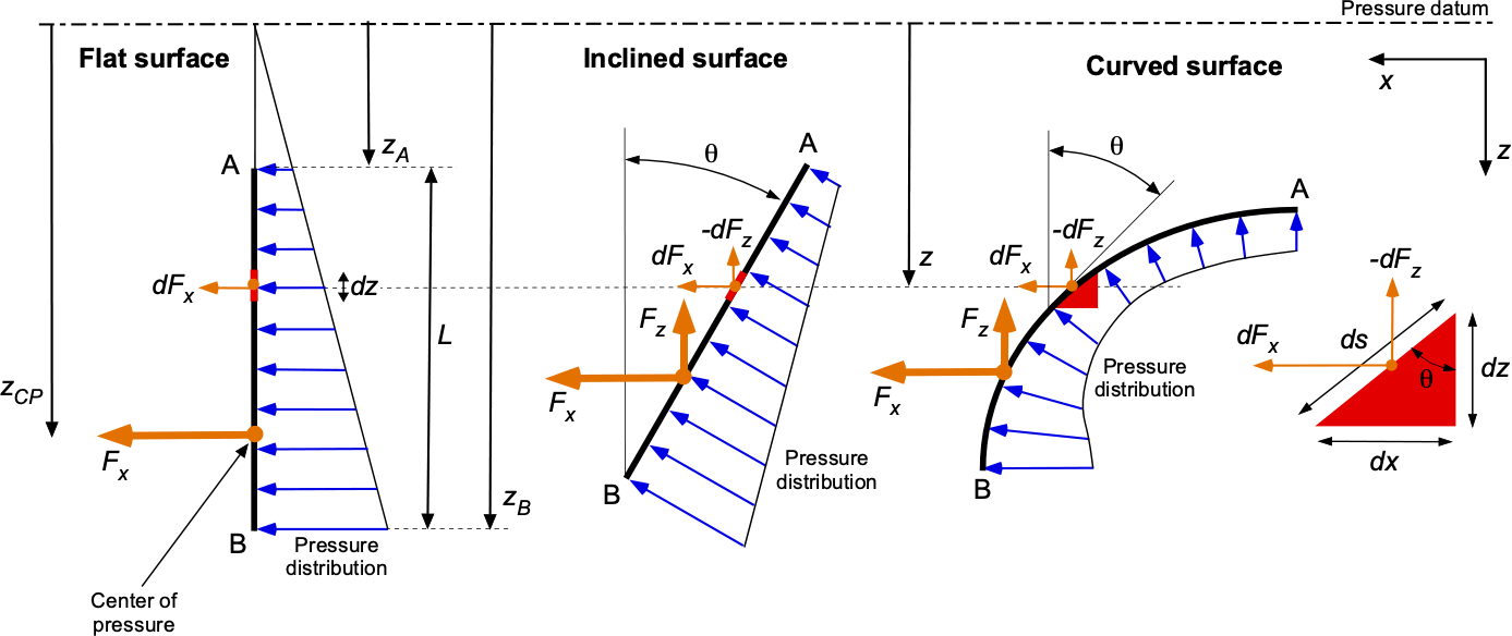
The summation of hydrostatic pressure forces acting over surfaces is a frequent problem in engineering. Such pressure distributions are typically non-uniform, so the net forces and moments acting on the surface must be obtained by integration. Consider the scenarios in the figure below, which shows the hydrostatic pressure distributions acting over a vertical flat surface, an inclined flat surface, and a curved surface.

Many engineering problems involve integrating pressures over submerged surfaces in a stagnant fluid, for which hydrostatic principles can be used.

Vertical Flat Surfaces

In the case of the vertical flat surface, the pressure force $dF_x$ acting on the elemental length $dz$ at depth $z$ from the pressure datum will be

(58) $\begin{equation*} dF_x = \varrho \, g \, z \, dz \quad \mbox{per unit length} \end{equation*}$

where per unit length means 1 unit into the screen/page. The total force acting on the surface will be

(59) $\begin{equation*} F_x = \varrho \, g \int_{z_A}^{z_B} z \, dz \quad \mbox{per unit length} \end{equation*}$

and performing the integration gives

(60) $\begin{equation*} F_x = \varrho \, g \left[ \frac{z^2}{2} \right]_{z_A}^{z_b} = \varrho \, g \left( \frac{ (z_A - z_B)^2 }{2} \right) = \varrho \, g \left( \frac{L^2}{2} \right) \quad \mbox{per unit length} \end{equation*}$

The center of pressure on the plate can be found by taking moments about the pressure datum, i.e.,

(61) $\begin{equation*} M = \varrho \, g \int_{z_A}^{z_B} z^2 \, dz \quad \mbox{per unit length} \end{equation*}$

and performing the integration gives

(62) $\begin{equation*} M = \varrho \, g \left[ \frac{z^3}{3} \right]_{z_2}^{z_1} = \varrho \, g \left( \frac{(z_2 - z_1)^3}{3} \right) = \varrho \, g \left( \frac{L^3}{3} \right) \quad \mbox{per unit length} \end{equation*}$

Therefore, the center of pressure (cp) will be at

(63) $\begin{equation*} z_{\rm cp} = \frac{M}{F_x} = \dfrac{ \left( \dfrac{L^3}{3} \right)} {\left(\dfrac{L^2}{2}\right)} = \dfrac{2 \, L}{3} \end{equation*}$

which is located at a depth that is 2/3 the length of the plate down from point A.

Inclined Flat Surfaces

In the case of an inclined flat surface, the pressure forces per unit length (or span) acting on the elemental length $dz$ at depth $z$ from the pressure datum will be

(64) $\begin{eqnarray*} dF_x & = & \varrho \, g \, z \, \sin \theta \, dz\\[6pt] -dF_z & = & \varrho \, g \, z \, \cos \theta \, dz \end{eqnarray*}$

The total force components acting on the surface will be

(65) $\begin{eqnarray*} F_x & = & \varrho \, g \sin \theta \int_{z_A}^{z_B} z \, dz \\[6pt] -F_z & = & \varrho \, g \cos \theta \int_{z_A}^{z_B} z \, dz \end{eqnarray*}$

The $\sin \theta$ and $\cos \theta$ terms are taken outside the integral because $\theta$ is a constant. Performing the integration gives

(66) $\begin{eqnarray*} F_x & = & \varrho \, g \sin \theta \left( \frac{L^2}{2} \right) \\[6pt] -F_z & = & \varrho \, g \cos \theta \left( \frac{L^2}{2} \right) \end{eqnarray*}$

The center of pressure (cp) on the plate (assume two-dimensional) can be found by taking moments about the pressure datum, as done previously, which in this case is

(67) $\begin{equation*} z_{\rm cp} = \left( \frac{2}{3}\right) L \, \cos \theta \end{equation*}$

The process can be extended for plates at any orientation in three-dimensional space.

Curved Surfaces

In the cases of curved surfaces, there are only exact solutions if the geometry lends itself to such, i.e., circular arcs. In this case, the angle terms must be held with the integral such that the total force components acting on the surface will be

(68) $\begin{eqnarray*} F_x & = & \varrho \, g \int_{z_A}^{z_B} z \, dx = \varrho \, g \int_{z_A}^{z_B} z \sin \theta \, dz \\[6pt] -F_z & = & \varrho \, g \int_{z_A}^{z_B} z \, dy = \varrho \, g \int_{z_A}^{z_B} z \cos \theta \, dz \end{eqnarray*}$

The net force is, therefore,

(69) $\begin{equation*} F = \sqrt{ F_x^2 + F_z^2} \end{equation*}$

Another approach is to perform the integration using the surface expressed in terms of its unit normal vectors, $\vec{n}$ , i.e.,

(70) $\begin{equation*} \vec{F} = \varrho \, g \iint_{A} \vec{z} \bigcdot \vec{n} \, dA \end{equation*}$

Check Your Understanding #5 – Moment on a submerged gate

The figure below shows that a heavy swinging gate acts as an over-pressure release valve. The gate is of length $L$ = 2 m and width $W$ = 4 m. Assume that the gate can freely pivot about the hinge, and there is a suitable gasket around the edges of the gate to keep things water-tight. The water is in a large tank that connects to the gate through a channel of height $H$ = 0.5 m. The gate must open if the height of the water, $h$ , exceeds 5 m.

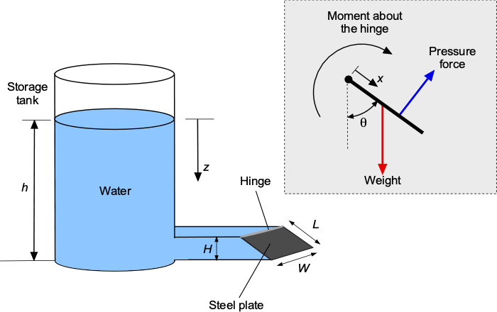Determine the equation describing the hydrostatic pressure force on the gate. Find the resultant moment ( torque) about the hinge from the action of the hydrostatic pressure on the gate. What thickness would be needed if the gate is made of solid plate steel (density = 7.5 grams/cm ${^3}$ )? Assume that the effects of air pressure on the gate can be neglected compared to the effects of water and that the density of water is $\varrho_w$ = 1,000 kg/m ${^3}$ .

Show solution/hide solution.

The hydrostatic pressure is a linear function of depth $z$ , i.e., $p = \varrho \, g \, z$ . Because the gate is at an angle, $\theta$ , to the vertical, the pressure force on the gate will depend on this angle. The lengths $H$ and $L$ are related by $H = L \cos \theta$ , where $\cos \theta = H/L$ = 0.5/2.0 = 0.25, so the angle $\theta$ is 75.5 $^{\circ}$ .

The hydrostatic pressure distribution acting over the gate along its length, $x$ , from the hinge will be

$p = \varrho_w g \big( (h - H) + x \cos \theta \big)$

The incremental hydrostatic force $dF_h$ on a short width (strip) of the gate $dl$ will be

$dF_h = p W dx = \varrho_w g \big( (h - H) + x \cos \theta \big) W \, dx$

and the corresponding incremental moment (or torque) $dM_h$ about the hinge will be

$dM_h= dF_h \, x = \varrho_w g \, W \big( (h - H) x + \cos \theta \, x^2 \big) \, dx$

Therefore, the total hydrostatic moment (or torque) $M_h$ about the hinge will be

$M_h = \int_0^L \varrho_w g \, W \big( (h - H)x + \cos \theta \, x^2 \big) \, dx$

which, after integration, becomes

$M_h = \varrho_w g \, W \bigg[ \frac{(h - H) x^2}{2} + \frac{\cos \theta \, x^3}{3} \bigg]_{0}^{L}$

and so

$M_h = \varrho_w g W \bigg( \frac{(h - H) L^2}{2} + \frac{\cos \theta \, L^3}{3} \bigg)$

Substituting values gives

$M_h = 1,000 \times 9.81 \times 4.0 \bigg( \frac{(10.0 - 0.5) 2.0^2}{2} + \frac{0.25 \times 2.0^3}{3} \bigg) = 771.73~\mbox{kNm}$

The weight $W_s$ of the steel gate will be

$W_s = \varrho_s L \, W \, t \, g$

where $t$ is the thickness of the plate. So, the gravity moment of the plate about the hinge will be

$M_s = W_s \left( \frac{L}{2} \right) \sin \theta = \varrho_{s} L \, W \ t \ g \left( \frac{L}{2} \right) \sin \theta$

If everything is just in a moment balance, then $M_s = M_h$ , so the needed thickness of the plate is

$t = \frac{M_h}{\varrho_s L \, W \, g \displaystyle{\left( \frac{L}{2} \right)} \sin \theta}$

The density of steel is 7.5 grams/cm ${^3}$ = 7,500 kg/m ${^{3}}$ . Also, $\sin \theta = \sin 75.52^{\circ}$ = 0.968. So, after substituting the numerical values, then

$t = \frac{771,730}{7,500 \times 2.0 \times 4.0 \times 9.81\displaystyle{\left( \frac{2.0}{2} \right)} 0.968} = 1.35~\mbox{m}$

So, a very thick and heavy steel gate is needed.

Piezometer Tube

A piezometer tube is a very simple device used to measure the static pressure of a fluid at a specific point in a pipe, tube, duct, or other application. The operation of a piezometer is based on the principle that the pressure at a point in a fluid is proportional to the height of the fluid column above that point, as shown in the figure below.

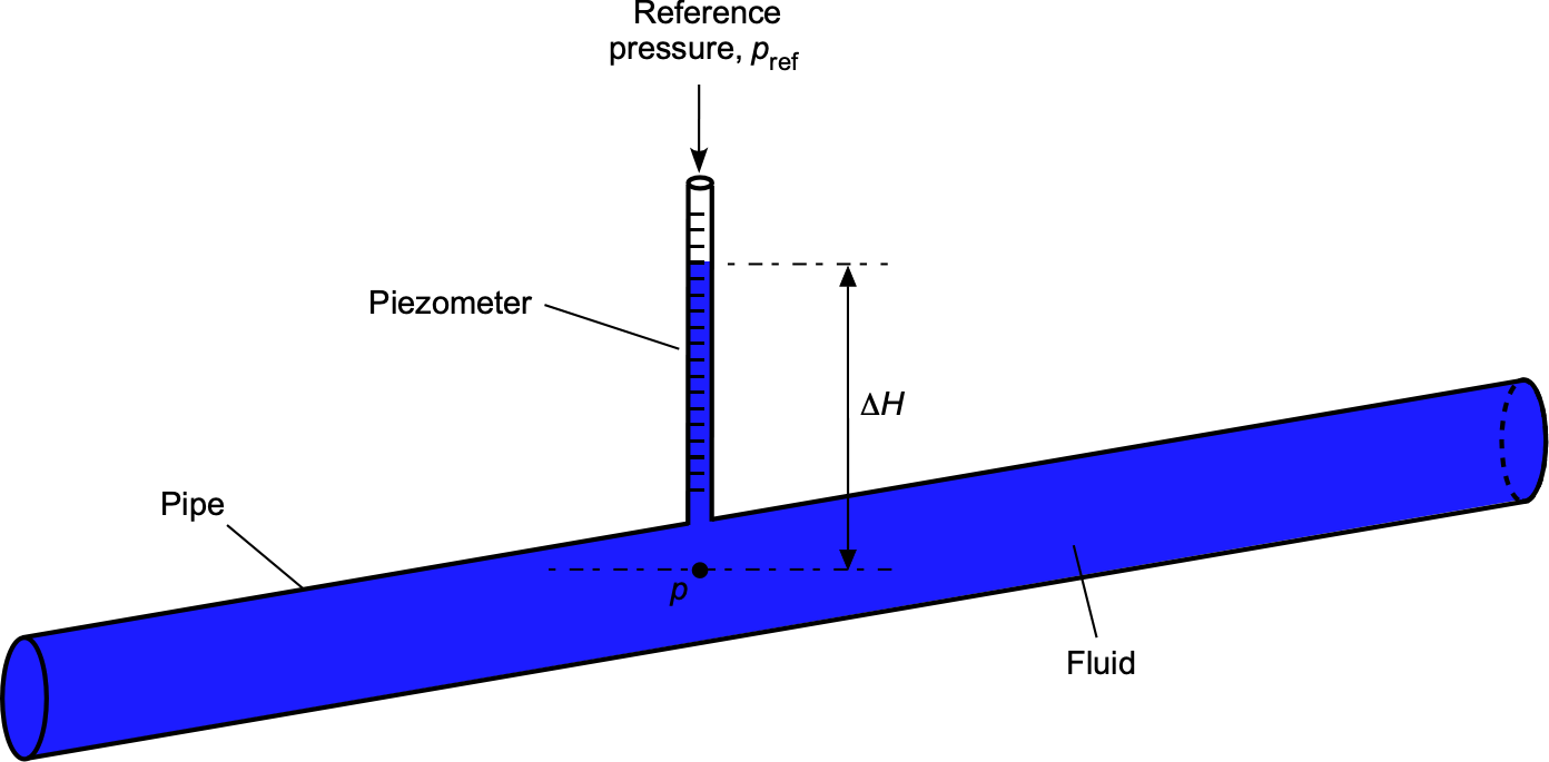
A piezometer is a simple device that measures pressure in terms of hydrostatic head.

The height measurement taken on the piezometer can be used to calculate the pressure head (or piezometric head) at the point of measurement. The pressure head, $\Delta H$ , is the difference between the external reference pressure, $p_{\rm ref}$ , and the pressure in the fluid, $p$ , and is given by

(71) $\begin{equation*} p - p_{\rm ref} = \varrho \, g \, \Delta h \end{equation*}$

where $p_{\rm ref}$ would usually be atmospheric (ambient) pressure, i.e., $p_{\rm ref} = p_{\rm atm}$ . The reading, therefore, is referred to as gauge (or gage) pressure. Piezometers are the simplest type of pressure measurement device. They work both with stagnant (stationary) and flowing fluids. Today, piezometers come in various types, including solid-state versions.

U-Tube Manometer

A U-tube manometer is the oldest and most basic type of pressure measuring instrument, and it is still used today as a reference instrument because of its inherent accuracy. A U-tube manometer is simply a glass tube with a “U” partially filled with a liquid, as shown in the figure below. This liquid, often called the manometric liquid, may be water, alcohol, oil, mercury (rarely used today), or some other liquid of known density. Light manometric liquids, such as water, measure small pressure differences, and heavier liquids are used for more significant pressure differences. This type of manometer has no moving parts and requires no formal calibration other than using an accurate length scale. The scale may be a simple ruler or something more sophisticated with a vernier scale.

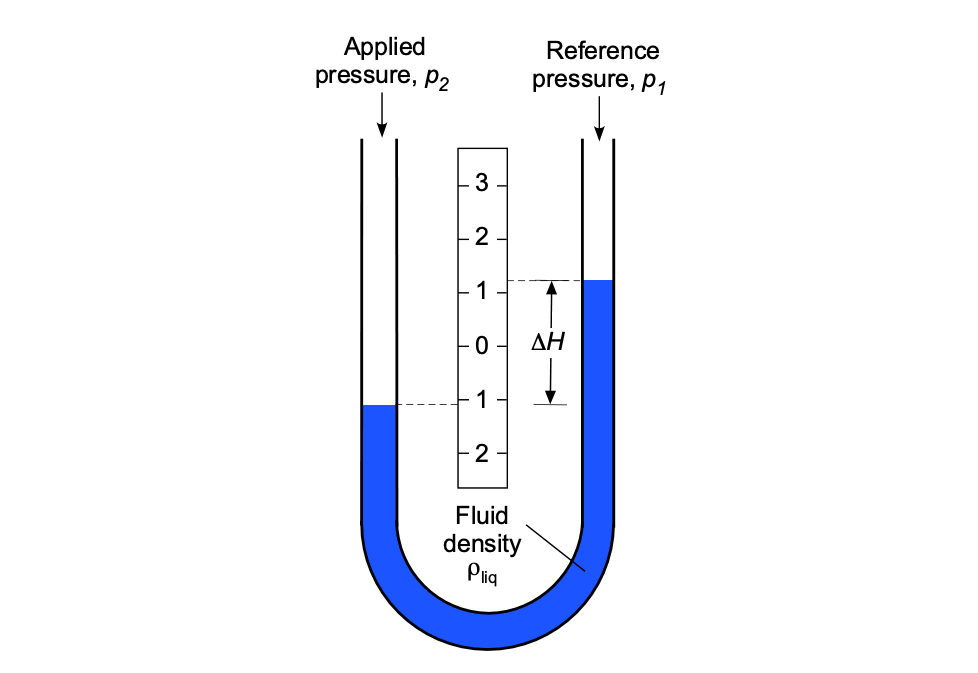
Operating Principle

The operating principle of liquid manometers is that they measure differences in pressure by balancing the weight of a manometric liquid contained between the two applied gas (or air) pressures. The height difference between the liquid levels in the U-tube’s two legs (or arms) is proportional to the air pressure difference, so the height (length) measurement can be related to the differential pressure value.

Using one arm of the manometer as a reference, such as $p_1$ , which could continue to be open to the atmosphere or connected to another (known) reference gas pressure, and connecting the other arm to an unknown applied pressure, $p_2$ m then the difference in the column heights, $\Delta h$ , is proportional to the difference in the two pressures, i.e.,

(72) $\begin{equation*} p_2 - p_1 = \varrho_{\rm liq} \, g \, \Delta H \end{equation*}$

where $\varrho_{\rm liq}$ is the density of the manometric liquid used in the U-tube. Notice that a pressure value measured with respect to atmospheric pressure is called gauge (or gage) pressure. If the reference pressure is a vacuum, then the pressure is referred to as absolute pressure.

The figure below summarizes what happens with the liquid levels in a U-tube manometer depending on whether the applied air pressure $p_2$ is greater than, equal to, or less than the reference pressure $p_{\rm ref}$ . For example, if the opening of each arm of a U-tube manometer is exposed to the same pressure, then the height of the liquid columns will be equal. Increasing the pressure applied to one arm or the other will produce a difference in the levels of the manometric fluid.

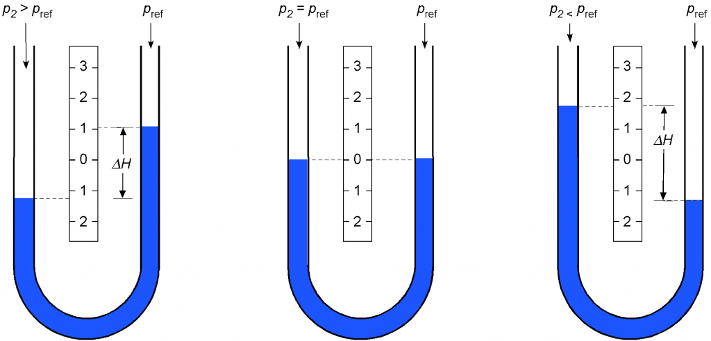
If one arm of a U-tube manometer is exposed to lower or higher pressures relative to atmospheric pressure, the liquid columns will rise and fall accordingly. If the opening of each arm of a U-tube manometer is exposed to the same pressure, then the height of the liquid columns will be equal.

Remember that a liquid manometer measures pressure in terms of a difference in the column heights of the manometric fluid, often expressed in units of inches or centimeters at a specific temperature. The height measurements are easily changed to standard pressure units using appropriate conversion factors, e.g., 1 inch of water equals 5.1971 lb/ft $^2$ or 0.0361 lb/in $^2$ .

“Rules” of Manometry

Several basic principles or “rules” of manometry directly follow when using the constant density solution to the aero-hydrostatic equation, i.e., p + $\varrho \, g \, z = \mbox{constant}$ . Learning how to use these rules properly is obtained by studying exemplar problems in hydrostatics. These rules are:

1. The pressure at two points 1 and 2 in the same fluid at the same height is the same if a continuous line can be drawn through the fluid from point 1 to point 2, i.e., $p_1$ = $p_2$ if $z_1$ = $z_2$ .
2. Any free surface of a fluid open to the atmosphere has atmospheric pressure, $p_a$ , acting upon the surface.
3. In most practical hydrostatic problems with air, the atmospheric pressure can be assumed to be constant at all heights unless the change in vertical height is significant, e.g., more than a few feet or meters.
4. For a liquid in a container, the shape of a container does not matter in hydrostatics, i.e., the pressure at a point in the liquid depends only on the vertical height of the fluid above it. This result is called the hydrostatic paradox.
5. The pressure is constant across any flat fluid-to-fluid interface.

Variations of U-tube Manometers

Many variations of the basic U-tube manometer concept include inverted, inclined, and reservoir or well-type manometers. All manometers respond to changes in pressure by vertical changes in fluid height.

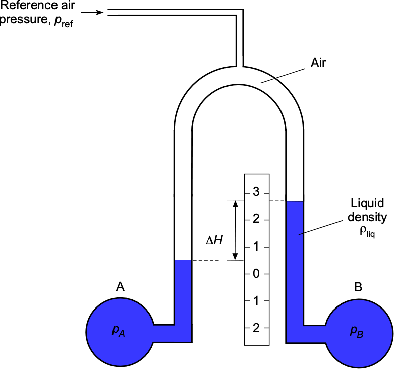
Inverted Manometer

An inverted U-tube manometer is often used to measure pressure differences in liquids. The space above the liquid in the manometer is filled with air at a known reference pressure, which can be adjusted to balance the liquid levels and vary the sensitivity of the manometer. When the pressure at B is higher than at A, the liquid in the U-tube is displaced, creating a difference in the liquid levels in the two arms of the tube. The difference in the liquid levels is directly proportional to the pressure difference between the two points, i.e.,

(73) $\begin{equation*} p_B - p_A = \varrho_{\rm liq} \, g \, \Delta H \end{equation*}$

Inverted U-tube manometers are often used to measure differences in pressure in liquids.

Asymmetric Manometers

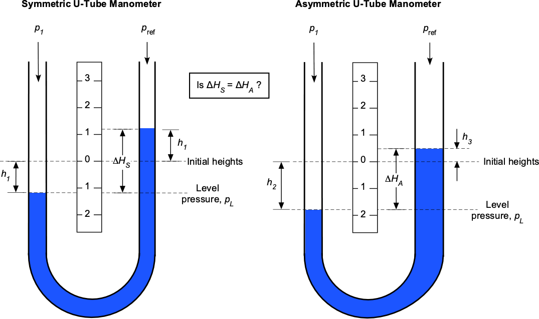
Asymmetric manometers are sometimes encountered, in which one arm of the manometer has a different cross-sectional area than the other arm, as shown in the figure below. The natural question that arises, therefore, is whether the difference in the two fluid levels is the same as that of a symmetric manometer for a given air pressure difference.

Symmetric U-tube manometer (left) and asymmetric U-tube manometer (right). Are the values of $\Delta H_S$ and $\Delta H_A$ equal for a given pressure difference?

In the case of the symmetric manometer, it will be apparent that for a given air pressure difference, $p_1 - p_{\rm ref}$ , the liquid level on the left arm will drop by the same amount, $h_1$ , as the level increases on the right arm, i.e., conservation of mass and volume (both are conserved for a liquid). Therefore, applying hydrostatic principles to the right arm of the symmetric manometer at level pressure gives

(74) $\begin{equation*} p_L = p_{\rm ref} + \varrho_{\rm liq} \, g \, h_1 + \varrho_{\rm liq} \, g \, h_1 = p_{\rm ref} + \varrho_{\rm liq} \, g \, 2 h_1 = p_{\rm ref} + \varrho_{\rm liq} \, g \, \Delta H_S \end{equation*}$

ignoring any hydrostatic effects of the air. Applying hydrostatic principles to the left arm of the symmetric manometer, then at level pressure

(75) $\begin{equation*} p_L = p_1 \end{equation*}$

Therefore,

(76) $\begin{equation*} p_1 - p_{\rm ref} = p_L - p_{\rm ref} = \Delta p = \varrho_{\rm liq} \, g \, \Delta H_S \end{equation*}$

In the case of the asymmetric manometer, the liquid level in the right arm will not rise as far compared to the symmetric manometer. However, to satisfy the conservation of volume, the level in the left arm must drop more, i.e., $h_2 > h_1$ and $h_3 < h_1$ . Applying hydrostatic principles to the right arm of the asymmetric manometer at level pressure, then

(77) $\begin{equation*} p_L = p_{\rm ref} + \varrho_{\rm liq} \, g \, h_3 + \varrho_{\rm liq} \, g \, h_2 = p_{\rm ref} + \varrho_{\rm liq} \, g \, ( h_3 + h_2 ) = p_{\rm ref} + \varrho_{\rm liq} \, g \, \Delta H_A \end{equation*}$

again ignoring any hydrostatic effects of the air. Applying hydrostatic principles to the left arm of the asymmetric manometer, then

(78) $\begin{equation*} p_L = p_1 \end{equation*}$

as before. Therefore, in this case

(79) $\begin{equation*} p_1 - p_{\rm ref} = p_L - p_{\rm ref} = \Delta p = \varrho_{\rm liq} \, g \, \Delta H_A \end{equation*}$

Finally, equating Eq. 76 obtained for the symmetric manometer and Eq. 79 for the asymmetric manometer gives

(80) $\begin{equation*} \Delta p = \varrho_{\rm liq} \, g \, \Delta H_A = \varrho_{\rm liq} \, g \, \Delta H_S \end{equation*}$

proving that $\Delta H_A$ is equal to $\Delta H_S$ for the same $\Delta p$ . The conclusion is that regardless of the cross-sectional areas of the arms of a U-tube manometer, a given applied differential pressure will create the same height difference on the liquid levels, even though the levels themselves will be different (conservation of mass or volume) compared to the case where the legs have the same area.

Well Manometer

The simple U-tube manometer has a significant disadvantage because the liquid levels in both arms must be read and recorded to calculate the pressure. By making the diameter of one arm much larger than the other, the manometric liquid level will fall very slightly on that arm compared to the more significant rise in the other arm. This principle is used in a well-type or reservoir-type of manometer, as shown in the image below, which is just another variation of the asymmetric manometer.

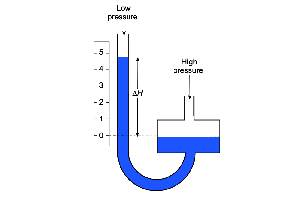
Well-type manometers are often used for reference pressure measurements or calibrations of other pressure-measuring devices.

In this case, the drop in the liquid level of the well can be ignored in any practical sense. The differential pressure can then be obtained in the standard way by measuring the change in the fluid level in the well relative to the vertical height of the column, i.e.,

(81) $\begin{equation*} \Delta p = \varrho_{\rm liq} \, g \, \Delta H \end{equation*}$

Some well manometers used for high accuracy may require a slight adjustment in that the scale’s datum can be moved to “zero” the reading relative to the well level. In either case, only one reading is required on the scale to determine the differential pressure. Well-type manometers are often used for measuring lower-pressure differentials or as calibration manometers, but they are not limited to such uses.

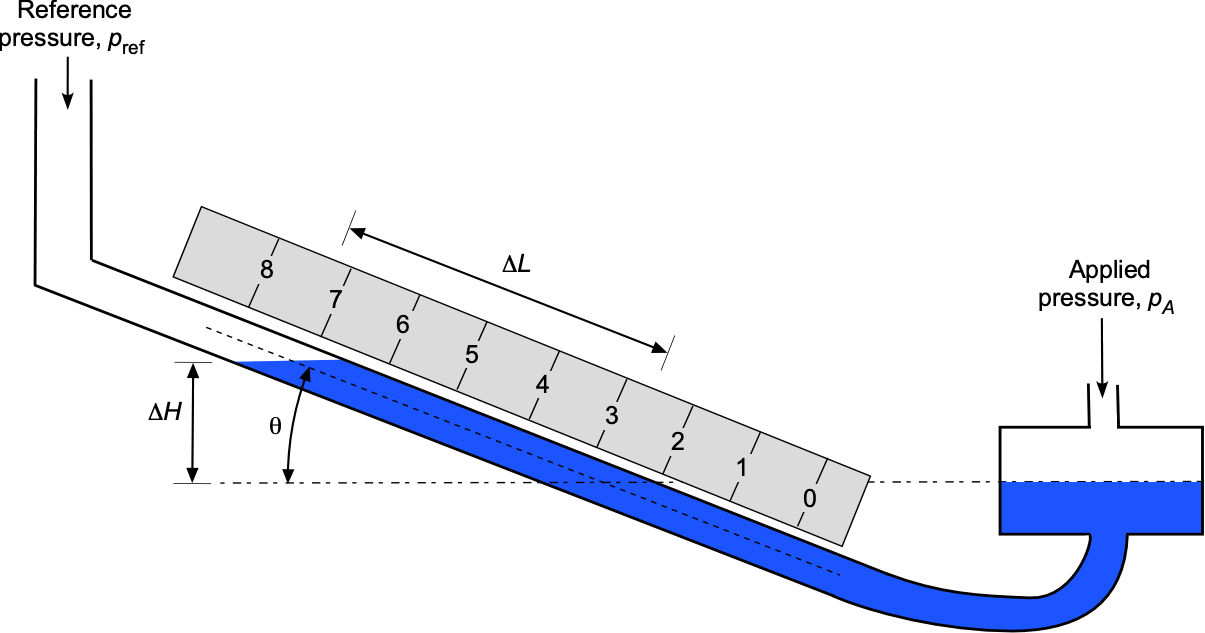
Inclined Manometer

With an inclined manometer arm, as shown below, a vertical change in the fluid levels is stretched over a longer length. Consequently, an inclined-arm manometer has better sensitivity for measuring lower pressures, i.e.,

(82) $\begin{equation*} p_A - p_{\rm ref} = \Delta p = \varrho_{\rm liq} \, g \, \Delta H = \varrho_{\rm liq} \, g \, \Delta L \sin \theta \end{equation*}$

This means that the length along the arm is “magnified” according to

(83) $\begin{equation*} \Delta L = \frac{\Delta H}{\sin \theta} \end{equation*}$

For example, if $\theta = 30^{\circ}$ then $\Delta L = 2 \Delta H$ . Because the fluid level moves further along the arm for a given pressure difference, it is easier to measure on the scale.

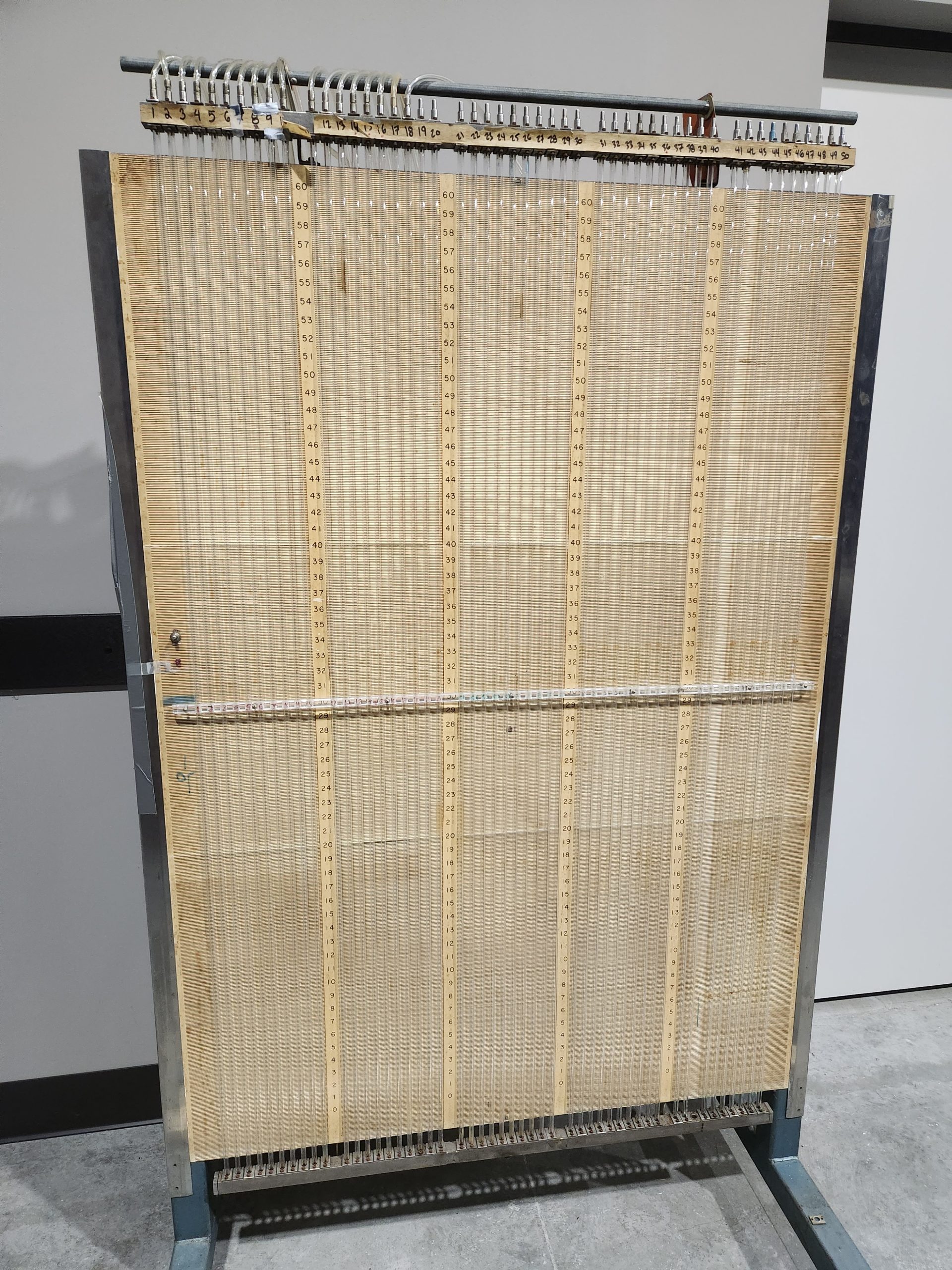
An inclined manometer causes an increased movement of liquid in the arm when the applied pressure changes, making it more sensitive.

Bank Manometers

Liquid manometers are helpful in many applications but have limitations because they are large, bulky, and more suited to a laboratory than routine use in the field. They also come in large banks suitable for use in the wind tunnel, as shown in the photograph below. One side of the manometer bank is referenced to static pressure through a plenum containing the manometer liquid (usually water with a dye in it), much in the way of a well-type of manometer, and each individual manometer is connected to a separate pressure tap, such as on a wing. The process is the same in that the pressure is proportional to the height of the fluid column, which can be read off on a scale. Such types of manometers, however, take a very long time to read and cannot be interfaced with a computer other than manually.

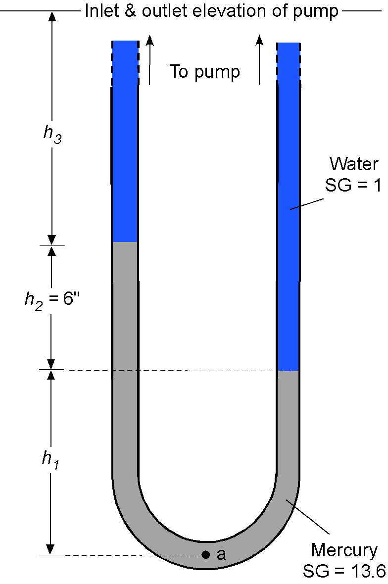
A liquid-filled manometer bank for use in the wind tunnel, which solid-state pressure transducers have now replaced.

Check Your Understanding #6 – Use of a U-tube manometer

A U-tube manometer is connected to the inlet and outlet of a water pump, as shown below; the left side is connected to the inlet at pressure $p_{\rm in}$ and the right side to the outlet at pressure $p_{\rm out}$ . Assuming that the inlet and outlet conditions are at the same elevation, determine the pump’s pressure increase. Remember that specific gravity SG = $\varrho/\varrho_{\rm H_{2}O}$ . The density of water can be assumed to be 1.93 slugs/ft ${^3}$ .

Show solution/hide solution.

The pressure at point “a” will equal the pressure produced by each arm of the U-tube manometer. For the left arm, then

$p_a = \varrho_{\rm Hg} \, g \, h_1 + \varrho_{\rm Hg} \, g \, h_2 + \varrho_{\rm H_{2}O} \, g \, h_3 + p_{\rm in}$

Similarly, for the right arm, then

$p_a = \varrho_{\rm Hg} \, g \, h_1 + \varrho_{\rm H_{2}O} \, g \, h_2 + \varrho_{\rm H_{2}O} \, g \, h_3 + p_{\rm out}$

Therefore, the difference in pressure becomes

$\Delta p = p_{\rm out} - p_{\rm in} = \varrho_{\rm Hg} \, g \, h_2 - \varrho_{\rm H_{2}O} \, g \, h_2 = \left( \varrho_{\rm Hg} - \varrho_{\rm H_{2}O} \right) g \, h_2$

or

$\Delta p = \left( SG_{\rm Hg} - SG_{\rm H_{2}O} ) \varrho_{\rm H_{2}O} \right) g \, h_2$

Substituting the known numerical values gives

$\Delta p = \left( 13.6 - 1.0 \right) \times 1.93 \times 32.17 \times (6.0/12) = 391.16~\mbox{lb/ft$^2$}$

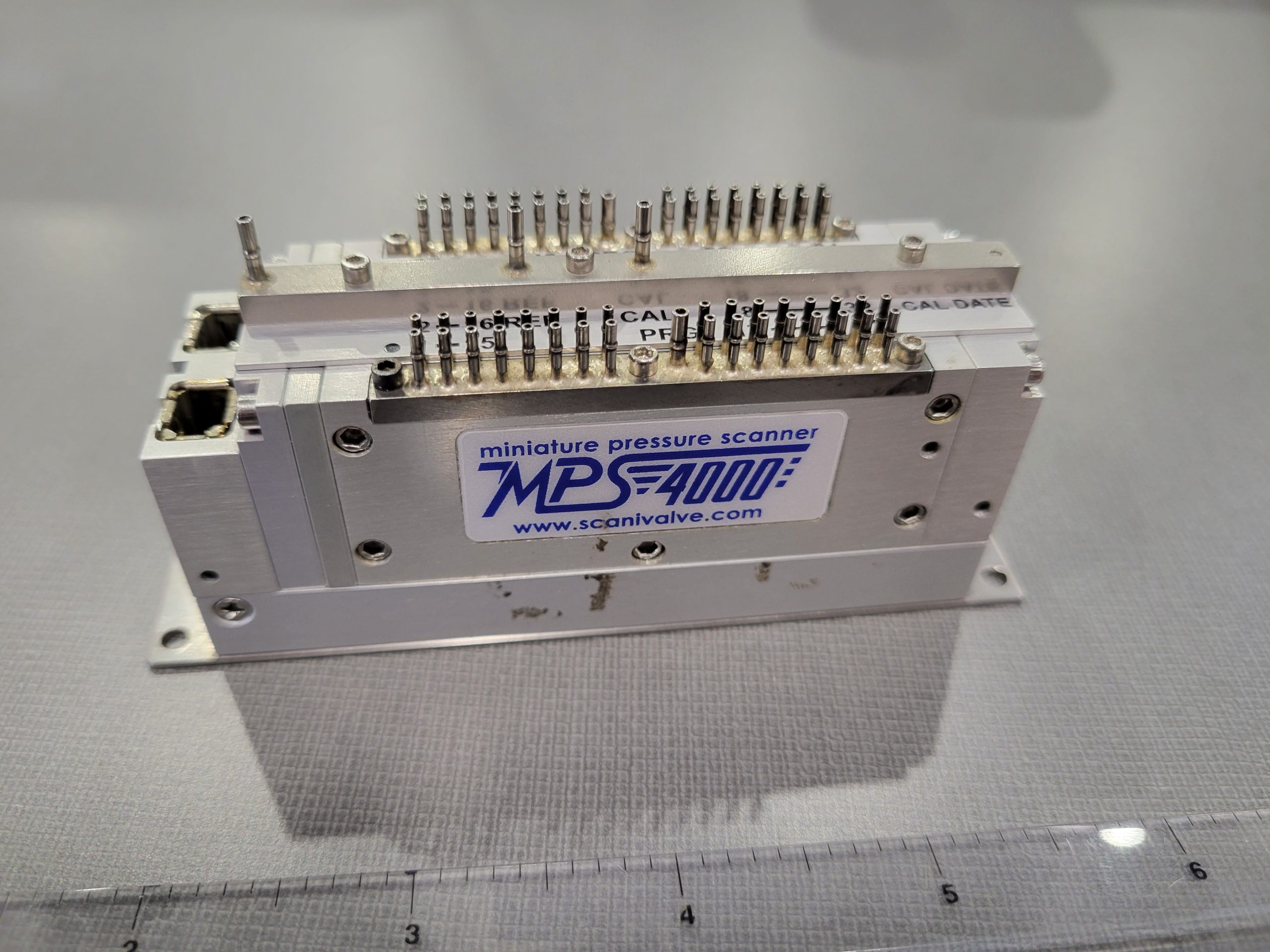
Pressure Transducers

The schematic below shows that a pressure sensor or pressure transducer is a solid-state device used for pressure measurement. A pressure sensor generates a voltage or other analog signal that is a function of the pressure imposed upon it. The sensor must be calibrated by applying known pressures and recording the output voltage; the resulting relationship is known as the calibration function. This relationship is usually linear, so a single constant or calibration coefficient represents the behavior. The sensor’s signal may also be conditioned by amplifying and filtering, then converting the signal to digital form through an analog-to-digital (A/D) converter before being stored on a computer.

Digital pressure manometers are also available in convenient, portable, battery-powered sizes for ease of use, with single or multiple inputs and outputs for controlling measurements and transferring data. In addition, calibrations or correction factors can be incorporated into the software used to manage the digital manometer. Today, pressure sensors are used in thousands of industrial applications and come in all sorts of sizes, shapes, and pressure ranges. Miniature pressure transducers are often used in aerospace applications because of their low weight and ability to be placed closely together, such as over the surface of a wing. In wind tunnel applications, pressure transducer modules, such as the one shown below, are often used. Pressure tubes can be connected to each of the ports, and the module has self-contained electronics that allow digital values of the pressures to be read directly by a computer and stored for analysis.

A miniature solid-state pressure transducer block allows 64 pressure values to be measured digitally at high data rates.

Hydraulic Press

A hydraulic press is a device that uses the basic principles of hydrostatics to allow a relatively small input force on a piston in a primary cylinder to be multiplied to give a much larger output force on a piston in a secondary cylinder. This concept is called mechanical advantage. It is used extensively in the design of hydraulic systems to produce larger mechanical forces where needed, as shown in the figure below. This approach can be used for tooling, various machinery, and on aircraft for landing gear, flaps, flight control surfaces, and brakes.

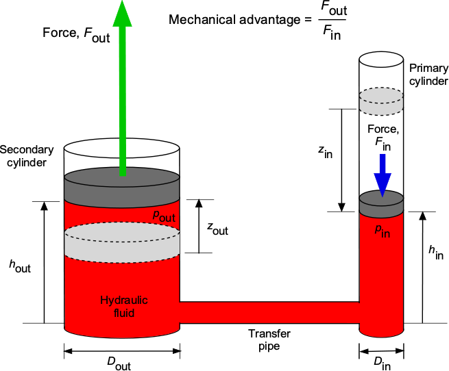
The fluid is some form of hydraulic oil, which can be considered incompressible, with density $\varrho_{\rm oil}$ . The system comprises two cylinders of different diameters, $D_{\rm in}$ and $D_{\rm out}$ , respectively, that are filled with the hydraulic fluid, each capped with tight-fitting pistons that slide inside the cylinders. The applied force, $F_{\rm in}$ , on the primary piston causes it to move downward (in this case), causing the fluid to move through a transfer pipe and into the secondary cylinder. The force on the primary piston also increases the pressure, which is transmitted hydrostatically to give the same change in pressure on the secondary piston. The secondary piston has a larger area, providing a larger force, $F_{\rm out}$ , for the same pressure.

Assume that the system is initially in hydraulic equilibrium with no forces on either of the pistons. The force $F_{\rm in}$ applied to the primary piston moves it down by a distance $z_1$ , increasing the pressure below the piston to

(84) $\begin{equation*} p_{\rm in} = \frac{F_{\rm in}}{A_{\rm in}} = \frac{F_{\rm in}}{\pi D_{\rm in}^2/4} = \frac{4 F_{\rm in}}{\pi D_{\rm in}^2} \end{equation*}$

On the secondary or output side, the pressure below the piston is

(85) $\begin{equation*} p_{\rm out} = \frac{F_{\rm out}}{A_{\rm out}} \end{equation*}$

Also, it will be apparent that because the pressures at the same height in the same fluid are equal, then

(86) $\begin{equation*} p_{\rm in} = p_{\rm out} - \varrho_{\rm oil} \, g \left( h_{\rm out} - h_{\rm in} \right) = p_{\rm out} - \varrho_{\rm oil} \, g \, \Delta h \end{equation*}$

Therefore, introducing the pressure values in terms of forces gives

(87) $\begin{equation*} \frac{4 F_{\rm in}}{\pi D_{\rm in}^2} = \frac{4 F_{\rm out}}{\pi D_{\rm out}^2} - \varrho_{\rm oil} \, g \, \Delta h \end{equation*}$

or

(88) $\begin{equation*} \frac{F_{\rm in}}{A_{\rm in}} = \frac{F_{\rm out}}{A_{\rm out}} - \varrho_{\rm oil} \, g \, \Delta h \end{equation*}$

If the difference in hydrostatic pressure head, $\varrho_{\rm oil} \, g \, \Delta h$ , can be assumed to be small compared to the pressure applied by the forces, which is easily justified, then $p_{\rm out} \approx p_{\rm in}$ , and so

(89) $\begin{equation*} \frac{F_{\rm in}}{D_{\rm in}^2} = \frac{F_{\rm out}}{D_{\rm out}^2} \mbox{~~~or~~~} \frac{F_{\rm in}}{A_{\rm in}} = \frac{F_{\rm out}}{A_{\rm out}} \end{equation*}$

This means that the output force on the secondary piston is

(90) $\begin{equation*} F_{\rm out} = F_{\rm in} \left( \frac{ D_{\rm out}^2}{D_{\rm in}^2} \right) = F_{\rm in} \left( \frac{ A_{\rm out}}{A_{\rm in}} \right) \end{equation*}$

Therefore, input force, $F_{\rm in}$ , will be multiplied by the ratio of the areas or square of the diameter ratios of the primary and secondary cylinders to give a higher output force, $F_{\rm out}$ . For example, if $A_{\rm out}/A_{\rm in} = 5$ , then $F_{\rm out} = 5 F_{\rm in}$ and so a mechanical advantage of 5.

Notice that the distance the primary piston must move in its cylinder is greater than the distance the secondary piston moves. The volume of fluid shared below the two pistons is conserved (oil is incompressible), i.e.,

(91) $\begin{equation*} z_{\rm in} \, A_{\rm in} = z_{\rm out} \, A_{\rm out} \end{equation*}$

so that

(92) $\begin{equation*} z_{\rm out} = \left( \frac{ A_{\rm in}}{ A_{\rm out}} \right) z_{\rm in} \end{equation*}$

If $A_{\rm out}/A_{\rm in} = 5$ , then $z_{\rm in} = 5 z_{\rm out}$ , so the primary piston must move five times as far, which is the price to pay for a mechanical advantage.

The problem can also be approached using the conservation of energy. The work done by the force on the primary piston must appear as work by the secondary piston, assuming no losses in the fluid transfer, i.e.,

(93) $\begin{equation*} F_{\rm in} \, z_{\rm in} = F_{\rm out} \, z_{\rm out} \end{equation*}$

Therefore, the same result of the multiplication of forces is obtained, i.e.,

(94) $\begin{equation*} F_{\rm out} = F_{\rm in} \left( \frac{z _{\rm out}}{z_{\rm in}} \right) \end{equation*}$

Summary & Closure

The principles of hydrostatics apply to stationary or stagnant fluids, i.e., those with no relative motion between the fluid elements. Therefore, these fluid problems are easier to understand and predict. The problems that can be analyzed using hydrostatics include buoyancy, finding pressures on submerged objects or inside fluid-filled containers, or any other fluid problem where the fluid is not in motion or stagnant. Besides pressure, other fluid properties of interest are temperature and density. The essential equations to remember are those for the hydrostatic pressure field and the aero-hydrostatic equation. The latter is a particular case of the former when gravity is the only acting body force. The equation of state is also helpful in analyzing hydrostatic problems, which can be used to relate pressures, densities, and temperatures in a gas. Another use of the aero-hydrostatic equation is to help analyze the properties of the Earth’s atmosphere and the atmospheres on other planets.

5-Question Self-Assessment Quickquiz

For Further Thought or Discussion

A balloon filled with helium is released at sea level. What happens to the balloon?
Can a lead balloon float? Be sure to explain any assumptions you may use.
A cylindrical container (bucket) filled with water is rotated. What happens to the shape of the water’s surface?
In a density-stratified water container, the density varies with depth according to $\varrho (z)$ = 1000 + 1.1 $z$ for 0 < $z$ < 100 m, where $z$ = 0 is the surface. Show how to determine the pressure field.
Sometimes, an inclined manometer is used to make pressure measurements. Explain why.
Explain the principle of a hydraulic lift for obtaining a large force from a small force.
A cruise ship weighs 100,000 tons. How much volume of seawater does it displace?
Precision liquid manometers are still used today, which may appear inconvenient if not old-fashioned. Explain why.
What factors influence the stability of floating objects? How can you determine the equilibrium position of a floating body and its stability conditions?

Additional Online Resources

To improve your understanding of hydrostatics, take some time to navigate to some of these online resources:

Wikipedia has a good site on hydrostatics.
Video on the concept of hydrostatic pressure from the University of Colorado.
Video on visualizing the idea of hydrostatic pressure.
For an interactive demonstration about hot air balloons, see: How do you control a hot air balloon?
For more on Archimedes and his principle, check out Eureka! The Archimedes Principle.
Pascal’s principle, hydrostatics, atmospheric pressure, lungs, and tires. Good lecture and demonstrations.
Hydrostatics, Archimedes’ Principle, what makes your boat float? Good lecture and excellent demonstrations.

Which may include translational, centrifugal, and Coriolis accelerations. ↵
These forces are significant in conducting fluids, such as plasmas and electrolytes. ↵
Archimedes is often considered as the father of this field. ↵

License

Icon for the Creative Commons Attribution-NonCommercial-NoDerivatives 4.0 International License

Introduction to Aerospace Flight Vehicles Copyright © 2022–2024 by J. Gordon Leishman is licensed under a Creative Commons Attribution-NonCommercial-NoDerivatives 4.0 International License, except where otherwise noted.

Digital Object Identifier (DOI)

https://doi.org/https://doi.org/10.15394/eaglepub.2022.1066.9