53 Astronautics, Space & Astrodynamics
Introduction[1]
Humankind has always strived to fly into space. Eventually, there comes a height above the surface of the Earth where the atmosphere starts to thin out so that airplanes can no longer fly there. This height is the beginning of what is known as outer space, which is usually referred to as space. The fastest and highest air-breathing propelled aircraft ever flown, the SR-71 Blackbird, achieved a speed of 3,540 kph (2,200 mph) at an altitude of 85,000 ft (about 26 km or 16 miles) before it ran out of atmosphere to fly as an aircraft. The rocket-powered North American X-15 achieved its maximum speed of 7,273 km/h (4,520 mph or Mach 6.7) and 107.8 km (67.1 miles), putting the aircraft well into the edge of space.
Why would humans, as firmly and well-established terrestrial beings, want to go up and outward into space and visit the stars? Space is a very unfriendly, if not hostile, environment for humans, with no air to breathe and ultra-high and ultra-low temperature extremes. Distances are enormous, and even the Moon, the closest planet to the Earth, is about 384,400 km (239,000 miles) away on average. Many will argue that human ventures into space waste time, money, and resources. Are proposed human missions to Mars just a fantasy? Perhaps limited resources are better spent on Earth-bound activities? Such arguments, however, are flawed and utterly contrary to human nature and the quest for scientific understanding.
Stephen Hawking, the renowned astrophysicist and the former Lucasian Professor of Mathematics at the University of Cambridge, spoke on “Why we should go into space” for NASA’s 50th Anniversary Lecture Series. Professor Hawking, now deceased, was severely disabled with ALS and eventually had to speak using a computer, but listen very carefully as to why he advocated the need to go into space, return to the Moon, and eventually make an attempt to go to Mars.
It soon becomes clear that if it were not for the development of rockets, satellites, and other space systems, humankind would know much less about their planet, and many “spinoff” technologies used in everyday life would never have been developed. For example, live weather, GPS, Google Maps, satellite television, the internet, battery-powered tools, and many things used daily would not exist! NASA has listed thousands of technological spinoffs from space activities that have benefited humans. The advances made in space exploration have also driven advancements in materials science, computer technology, and medicine, among others. As NASA says: “There’s more space in your life than you think!”
Learning Objectives
- Appreciate the challenges of humankind reaching into space.
- Learn about the history of astronomy and the planets.
- Understand the fundamental laws of satellite motion and spaceflight dynamics.
- Be able to distinguish between different types of orbits.
- Use Kepler’s equations to predict the motion of a satellite.
- Know how to transfer spacecraft between orbits.
- Understand the challenges of interplanetary travel, such as a mission to Mars.
Definition of Space
Theodore von Kármán rationalized that space must begin where the atmosphere’s density becomes asymptotically thin to create any aerodynamic lift on a flight vehicle. This height boundary between the world of “aeronautics” and atmospheric flight vehicles and that of “astronautics” and space vehicles has been defined as 100 km (about 62 miles or 328,000 ft); it has since become known as the Kármán line. Although there is no clear physical divide between the two, the Kármán line provides a convenient point of reference for aerospace engineers to differentiate between the two realms of flight.
It is much quoted that space is “The Final Frontier.” However, the reality is that it is only the next frontier, and the final frontier of the universe is still very much unknown. So, where does the universe end? Is there even an end that can be identified? What is out there? The answers to these questions pose some of the greatest mysteries of science. The prevailing theory is that the universe is still expanding and has no defined boundary or final frontier. However, this idea is still being explored and tested; new discoveries could challenge current understanding.
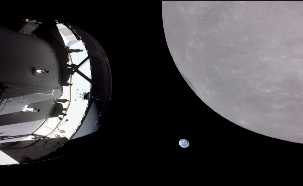
The vastness of space and the universe as a whole is best summed up by a quote about the Earth from the extraordinary scientist, astronomer, and professor Dr. Carl Sagan: “On it is the aggregate of everything we know since the beginning of time, and a tiny stage in the vastness of the cosmic arena.” The recent photograph of the Earth taken from the Orion spacecraft, as shown below, eminently makes the point. Despite the many technological advancements and understanding, the knowledge of the universe is still limited, and it remains an enigma in many ways. As shown below, the photograph of Earth taken from space is a humbling reminder of Earth’s small place in the cosmos. It inspires humankind to continue exploring and learning more about space and the universe.
What is Out There?
Humans have roamed the Earth for 300,000 years, but civilization has only existed for about 10,000 years. This time is a mere blink of an eye in the time scales of the universe, which is estimated to be over 14 billion years old, i.e., human civilization has been around for only about 0.0000001% of established time. Advancing technology is one of the most characteristic of all human activities; the fascination with the stars and the exploration of the universe is just one motivation. However, only in the last 500 years has humankind started to make more sense of its place in the universe, thanks to significant advancements in science, astronomy, engineering, and space flight. The study of the planets is called astronomy, and the study of space and the universe (the cosmos) is called cosmology.
There are billions upon billions of galaxies containing billions of planets; this is well known based on what can be seen from space telescopes. Therefore, it is impossible to rationalize the true scale of the universe. But are there also other civilizations on those planets? It seems likely that humans are not the only living things in the universe. Might humans one day see intelligent living beings arrive from another world? Will they look like humans? Most likely not – the randomness of evolution suggests that they will be very different from us. Maybe Earth has already been visited by extraterrestrial beings? However, while some believe in extraterrestrial visits based on anecdotal evidence, no solid scientific proof exists to support these claims. Further research and exploration of the universe are needed to answer these questions and better understand the possibilities of extraterrestrial life and other civilizations.
Geocentrism
The earliest contributors to the science of the universe and space included observations of the planets by the Greek philosopher Aristotle. Aristotle’s religious beliefs influenced his views on cosmology, but they were also based on scientific understanding and the celestial observations available at the time. However, his idea of a stationary Earth at the center of the universe, called geocentrism, was later disproved by Galileo and other scientists who used telescopes to observe the movements of the stars and the planets. The astronomer Claudius Ptolemaeus also believed the Sun, Moon, and other planets circled the Earth.
Heliocentrism
It is now well understood that the Earth is not at the center of the universe and that it orbits around the Sun as part of our solar system. However, Aristotelian cosmology and geocentrism dominated astronomy and science for millennia. Advancements in technology and scientific understanding gradually led to its rejection. In the 16th and 17th centuries, astronomers such as Copernicus, Galileo, and Kepler started to provide more evidence of heliocentrism, the idea that the Earth and other planets revolve around the Sun.
In 1532, the Polish astronomer Nicolaus Copernicus was the first to propose that the Sun was the central focus around which the planets rotated in circular orbits, the Earth turning once daily on its axis. Copernicus’s heliocentric model of the universe significantly departed from the widely accepted geocentric model and sparked a paradigm shift in scientific thinking. His work challenged the prevailing views of the time and paved the way for further advancements in astronomy and science.
The Scientific Revolution brought about by these advancements led to discoveries, theories, and insights into the nature of the universe and helped lay the foundations for modern science. The works of Galileo, Brahe, Kepler, and Newton, among others, built upon Copernicus’s ideas and expanded our understanding of the solar system and the universe.
Celestial Observations of Galileo
The Italian astronomer and scientist Galileo Galilei supported Copernicus’s theories that the Earth rotated on its axis once every 24 hours and simultaneously revolved around the Sun once a year. Starting in 1609, Galileo built on the concept of a spyglass or monocular to develop various astronomical telescopes with increasing magnifications. Galileo played a vital role in the Scientific Revolution by using telescopes to observe the heavens and gather empirical evidence supporting heliocentrism. He made numerous important discoveries, including the observation of four large moons orbiting Jupiter and the phases of Venus, which provided further evidence for the Copernican system.
Galileo made many vital contributions to science and astronomy and is considered one of the most outstanding scientists in history. His observations of celestial objects were groundbreaking and challenged long-held beliefs about the nature of the universe. Galileo discovered that the surface of the Moon was not smooth and was made of many craters from the impacts of asteroids, nor was it translucent, a common belief at that time. His study of sunspots was also significant and helped establish the idea that the Sun was not perfect and unchanging, as previously thought. Galileo’s use of the telescope to make detailed observations of the sky revolutionized astronomy and paved the way for future discoveries.
For these reasons, Galileo is known as the “Father of Observational Astronomy,” a title first assigned by Albert Einstein. His legacy continues to inspire scientists and astronomers. His book, Sidereus Nuncius (Sidereal Messenger), was published in 1610 and contains the results of Galileo’s early observations of the planets.
Kepler’s Laws of Orbital Motion
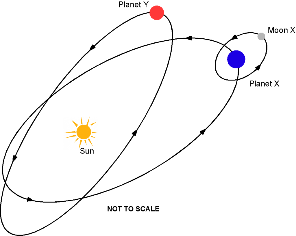
The 17th-century German astronomer Johannes Kepler, a student of Tycho Brahe, made the profound observation that the planets moved around the Sun in elliptical orbits, not circular orbits, as shown in the schematic below. This discovery was a significant departure from the previously held views. It helped establish that scientific and mathematical laws could explain the universe’s behavior.
Kepler’s laws provided a basis for the work of later scientists, including Isaac Newton, who used these laws to develop his laws of gravitation and describe the behavior of all objects in the universe, not just the planets. The true significance of Kepler’s work seemed only recognized once Newton rediscovered it. Kepler’s work, however, was a significant step towards a more complete understanding of the solar system and the universe as a whole and continues to influence astronomical research.
What is the closest planet to Earth besides the Moon?
Most people will say that the closest planet to Earth is Mars. But the closest planet to Earth, on average, is Venus. The average distance between Earth and Venus is about 41 million km (25.2 million miles), while the closest distance between the two planets is about 38 million km (23.6 million miles). Mercury is closer to the Sun than Earth and is, on average, 77 million km (48 million miles) away from Earth. However, because of its elliptical orbit, the distance between Mercury and Earth can vary significantly.
Kepler’s laws, published between 1609 and 1619, were not immediately accepted. Indeed, Galileo himself questioned Kepler’s observations and disregarded his book Astronomia nova. In English, the full title of Kepler’s book is “New Astronomy, Based upon Causes, or Celestial Physics, Treated by Means of Commentaries on the Motions of the Star Mars, from the Observations of Tycho Brahe.” Kepler’s laws were later confirmed by other astronomical observations, particularly the transit time projections of Venus and Mercury across the face of the Sun. However, these observations are now only of historical significance.
Kepler’s laws provided the foundation for the laws of gravitation developed by Isaac Newton, which are still used in modern celestial mechanics. Since then, Kepler’s laws have significantly impacted our understanding of the solar system and have been instrumental in space exploration and satellite navigation. Kepler’s Astronomia Nova soon became one of the most essential books in the history of astronomy, and Kepler’s work remains relevant in modern astrophysics and planetary science.
Kepler’s next book, “Epitome Astronomiae Copernicanae” or Epitome of Copernican Astronomy, was read widely by astronomers during the 17th century. However, his book’s publication was delayed until after Kepler’s death because of its “controversial” content in the eyes of the church. Nevertheless, many established astronomers and scientists of the era continued to challenge Kepler’s theories as a physical basis for explaining planetary and other celestial motions.
Newton & the “Principia”
Several other physical theories on planetary motions were developed from Kepler’s work. These theories culminated with the publication of Isaac Newton’s definitive Philosophiæ Naturalis Principia Mathematica in 1687. In this book, Newton explained the movement of orbiting planets in terms of the Sun’s gravitational attraction. In addition, he applied his laws of motion to re-derive Kepler’s laws of planetary motion in terms of a universal law of gravitation, a mathematical challenge later known as “Kepler’s Problem.” Over the centuries, countless astronomical observations and experiments have confirmed Kepler’s work and Newton’s law of gravitation. Indeed, Kepler’s laws have proved to be a cornerstone of modern astronomy and have contributed significantly to our understanding of the cosmos.
Defining Space
The aerodynamic environment in which aircraft fly has been well studied, and standardized mathematical models of the atmosphere up to the edges of space have been developed. The question now is how to describe the space environment. Many would claim that space is a vastness of absolute nothingness with no properties, but this is untrue.
Vastness of Nothingness?
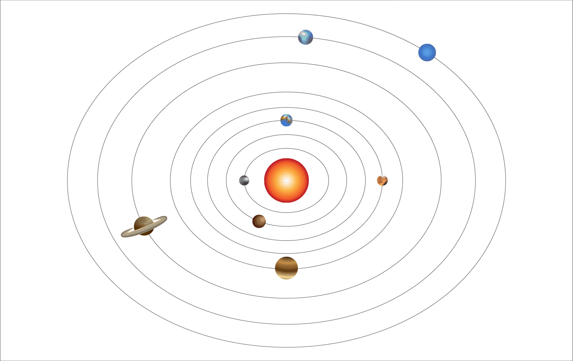
Space is an almost perfect vacuum at extremely low pressures and temperatures but primarily devoid of matter. Unlike air and other gases, space does not impede the motion of objects, and they have no drag as they move through space. However, small amounts of gases, dust, and other matter still float around in the vastness of the empty regions. Therefore, concepts such as pressure, temperature, and thermal transfer still have meaning in space, and concepts such as radiation also need to be considered. In other regions, matter can accumulate to form planets, stars, and galaxies; the Earth is just one of these lucky regions, along with a cluster of other planets in the solar system, which is shown in the animation below.
Space is also filled with various forms of radiation and electromagnetic fields, such as cosmic rays, solar winds, and magnetic fields. These radiation fields can affect the behavior of spacecraft and other objects in space and must be considered when designing spacecraft and planning space missions. The study of the space environment, known as space physics, also involves understanding the interactions between these various forms of radiation and other matter in space and how they influence the behavior of objects in the solar system. Space physics enables successful space missions, from communication and navigation to scientific exploration and human space flight.
Quantifying Vastness
Space and the universe are vast, extending enormous distances from the Earth. But the vastness of space can be measured! These measurements can be performed using radar because it is known that the speed of light, which in astronomy is given the symbol  , has an established value of 299,792,458 m/s (983,571,056 ft/s) or about 300,000 km/s (186,000 miles/s)! To put this in perspective, the speed of light is extremely fast, about one million times the speed of sound in the air on Earth.
The value of the speed of light can be used to confirm that the Earth is, on average, 384,400 km (239,000 miles) from the Moon, and the Earth is also 310.6 million km (193 million miles) from the Sun. That does not sound too far until you realize that the diameter of the Earth is only 12,741.2 km (7,917 miles), so the Moon is about 30 Earth diameters away, and the Sun is 24,378 diameters away!
This reason is why scientists and engineers measure immense space distances in light-years, the distance that light can travel in one year, which is equivalent to about 10 trillion km (6 trillion miles)! Yes, space is most definitely vast. However, the preferred unit of distance in astrometry is the parsec, given the symbol “pc,” which is defined as the distance at which an object will appear to move one arcsecond of parallax when the observer moves one astronomical unit perpendicular to the line of sight to the observer. One parsec is equal to approximately 3.26 light-years.
Planet Earth
From the understanding of the vast size and complexity of the universe, the Earth is just another tiny planet among billions of others. The Earth is part of a galaxy, part of an arm of a massive collection of stars swirling through space and throughout the universe. Indeed, our galaxy, the Milky Way, is estimated to be just one of the trillions of galaxies in the universe. Groups of galaxies are found to be arranged in clusters, and clusters then become part of superclusters. These superclusters stretch thousands of light-years across the universe, interspersed with dark voids and other features like black holes.
Our galaxy contains about 400 billion stars and is about 100,000 light-years from end to end. The neighboring Andromeda galaxy is over 220,000 light-years from end to end. It is estimated that there could be as many as 40 billion Earth-sized planets, even within our galaxy. Eleven billion of these estimated planets may be orbiting Sun-like stars, and some could have intelligent life. Alpha Centauri, the Earth’s nearest Sun-like star system, is 4.37 light-years away.
What exactly is a “light-year”?
A light-year is the distance light travels in one year, given the symbol “ly.” Light travels through space at about 300,000 km per second (186,000 miles per second) and covers approximately 9.46 trillion km (5.88 trillion miles) annually. Light-time is to measure the vast distances of space; nothing travels faster than light. Earth is about eight light minutes from the Sun, which is very close for a celestial body. A journey to the nearest star system, Alpha Centauri, would take over four years, even traveling at the speed of light, which is currently impossible according to the current understanding of physics. To put it into perspective, the Parker Solar Probe, the fastest spacecraft ever launched by humanity, takes about 90 years to travel one light-year at its maximum speed. These vast distances, combined with the long time it takes for light to travel from distant objects, make it a challenge to explore and understand the universe beyond our solar system.
What is Astrodynamics?
Astrodynamics, sometimes called “orbital mechanics,” is a critical engineering field encompassing the design and control of spacecraft missions. It involves applying mathematical and physical principles to understand and predict satellite motion, calculate spacecraft trajectories, determine orbits, and control spacecraft. The field is extensive, and this ebook can only begin to introduce the subject.
The study of astrodynamics is also crucial for many aspects of space exploration, from designing interplanetary missions to maintaining satellites in orbit for communication, navigation, and other purposes. Astrodynamic principles are used to determine the types of needed propulsion systems, propellant requirements, and control strategies required to put a satellite into orbit, keep it there, and maneuver it to achieve the mission goals.
Getting into Space
Rockets or launch vehicles send satellites, space probes, and human-carrying spacecraft into orbit around the Earth. A representative launch profile of a rocket is shown in the figure below. At the moment of the initial launch, the thrust produced by the rocket engine(s) will be greater than the vehicle’s weight, so the rocket accelerates away quickly from the pad. The rocket’s weight rapidly decreases because of the high propellant consumption rate, so it accelerates as it gains altitude. It also begins to pitch over to a more horizontal flight path under the effects of gravity, so the rocket quickly gains translational velocity. Finally, as it exits the atmosphere at about 60,000 ft (approximately 20 km), it will fly at supersonic speeds.
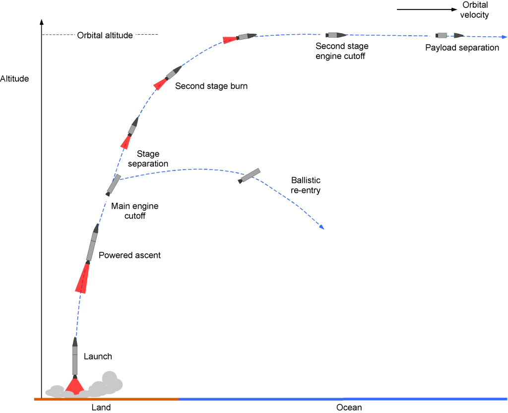
A few minutes into the ascent, staging will occur on the rocket booster, where the first stage is jettisoned as it runs out of propellant, and the second stage’s rocket engine(s) is ignited. The empty first stage then falls back toward the surface and either burns up in the atmosphere (depending on the staging altitude) or breaks up and crashes into the ocean. In exceptional cases, the first stage may be recovered; solid rocket boosters are usually recovered by parachute and may be reused.
After reaching orbit, the payload is on its own, traveling thousands of kilometers per hour as it orbits the Earth. The payload can then be configured to perform its intended mission, whether deploying satellites, conducting scientific experiments, or even transporting astronauts to the International Space Station. The complexity of the launch, ascent, and orbital insertion processes highlights the importance of having a highly skilled and knowledgeable engineering team, a thorough understanding of the atmospheric and space environment, and the use of reliable and tested technologies to ensure the success of a rocket launch, which are also very expensive.
Gravitational Laws of Attraction
The payload (e.g., a satellite) stays in orbit because it has been given momentum and kinetic energy by the chemical energy liberated in the propellant by the rocket engines. In orbit, the balance of forces can be explained using the principles of statics and dynamics. There will be an outward-directed force called centrifugal force, which must be balanced by an inward-directed force caused by the effects of gravitational attraction toward the Earth for equilibrium. This balance between gravity and centrifugal forces keeps the satellite orbiting around Earth, and any change to this balance of forces will cause it to either fall to Earth or escape into space.
It is often said that Isaac Newton was responsible for discovering gravity. The legend is that he was eating his lunch under a tree at his mother’s house in 1666 when an apple fell on his head. Even Newton himself was happy to go along with this story if he were to give himself claim to the discovery of gravity. Although Isaac Newton is widely credited with formulating the laws of gravity, Robert Hooke had previously established the concept of a gravitational force and its attraction between bodies. However, Newton provided a robust mathematical framework for understanding gravity and formulated the law of universal gravitation, so most of the credit goes to Newton.
Universal Law of Gravitation
Hooke and Newton understood that the “force of gravity” between two masses must be related to the magnitude of the masses and the distance between them, i.e., the bigger they are and the closer they are, the stronger the mutual force between them. They both hypothesized that this force of attraction,  , will be directly dependent upon the product of the masses of both objects, i.e.,
  and
and  , respectively, and inversely proportional to the square of the distance that separates their centers of masses, i.e.,
(1) 
where  is the distance between the centers of the two masses, as shown in the figure below.
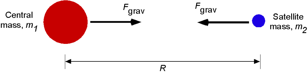
Newton went further and determined that there must exist a universal constant proportionality,  , such that
(2) 
Equation 36 is called the Universal Law of Gravitation. The minus sign denotes that this force is attractive, i.e., the masses are attracted toward each other. Despite its simplicity, this fundamental work established Isaac Newton as one of the most influential scientists in history.
Gravitational Constant
Newton did not live long enough for him to determine the numerical value of the universal gravitational constant, . Its value was subsequently determined by Henry Cavendish, who measured the average density and the Earth’s mass,  , which is
  kg, and then deduced the value of . The accepted modern value of the universal gravitational constant is
  N m
N m kg
kg .
.
Consequently, Eq. 36 is often redefined for the Earth as
(3) 
where  is the mass of the orbiting body of the Earth. In this case,
  is called the Earth’s gravitational constant, i.e.,
(4) 
It is important to remember that the value of  will vary from planet to planet.
Value of Acceleration Under Gravity
Everyone knows that gravity’s effects on the Earth’s surface are equivalent to an acceleration of 9.81 m/s2 (or 32.17 ft/s2), which is given the symbol  . The question is: Where does this value come from? Its value is easy to determine using the universal law of gravitation, which states, in general, that
(5) 
so for a mass on the surface of the Earth and using Newton’s second law that  , then
(6) 
where is the Earth’s mass and  is its radius. The Earth is not exactly a sphere but an oblate spheroid with an equatorial bulge. However, the assumption that the Earth is a sphere is close enough for this analysis, as shown in the figure below.
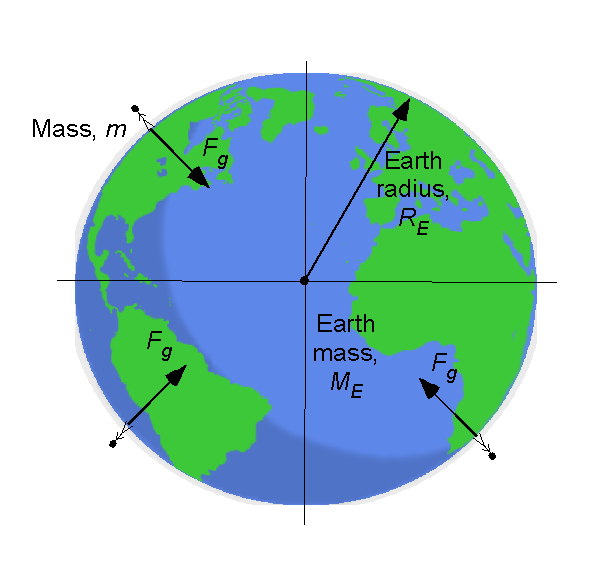
Recall that the Earth’s mass, , is kg, the radius of the Earth is  m, and the universal gravitational constant is N m kg. Therefore, rearranging Eq. 6 gives
(7) 
Substituting the known values gives
(8) 
As might be expected, the familiar value of comes from the direct application of the universal law of gravitation to a mass on Earth’s surface. Because of the use of in various problems in orbital mechanics, the symbol  is often used.
Check Your Understanding #1 – Your weight on another planet?
You are fortunate to be an astronaut sent out to explore planet X. This planet has a mass that is four times greater than the Earth and three times its radius. How will the “force of gravity” feel to you on planet X compared to when you are on Earth?
Show solution/hide solution.
Using the universal law of gravitation gives
![\[ F_{\rm Earth} = \frac{G \, M_{\rm Earth} \, m_{\rm You}}{R_{\rm Earth}^2} \]](https://eaglepubs.erau.edu/app/uploads/quicklatex/quicklatex.com-bd2a13feec78dcbaf7bdafa9e771967d_l3.svg "Rendered by QuickLaTeX.com")
The contribution of planet X’s mass will change your weight compared to Earth’s. Therefore, in this case,
![\[ F_{\rm X} = \frac{G \, M_{\rm X} \, m_{\rm You}}{{R_{\rm X}}^2} \]](https://eaglepubs.erau.edu/app/uploads/quicklatex/quicklatex.com-cc5e68209bc797c7caaa427707d812d5_l3.svg "Rendered by QuickLaTeX.com")
Substituting the specified information gives
![\[ F_{\rm X} = \frac{G \, 4 M_{\rm Earth} \, m_{\rm You}}{3 \, R_{\rm Earth}^2} \]](https://eaglepubs.erau.edu/app/uploads/quicklatex/quicklatex.com-1eb3566d4894e3d79bef9429b87f00eb_l3.svg "Rendered by QuickLaTeX.com")
so that
![\[ F_{\rm X} = \frac{4}{9} F_{\rm Earth} \]](https://eaglepubs.erau.edu/app/uploads/quicklatex/quicklatex.com-048e56dd0a8a65bedbe0c80ff8d5fca4_l3.svg "Rendered by QuickLaTeX.com")
Therefore, the force of gravity you will experience as an astronaut on planet X would be approximately 1.78 times greater than the force of gravity experienced on Earth. This means you would weigh about 1.78 times more on planet X than on Earth.
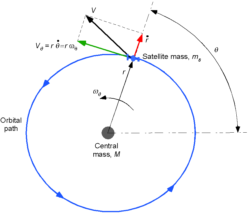
Circular Orbits
Consider a satellite in a circular orbit around the Earth. Circular orbits arise whenever the gravitational force on a satellite balances the centrifugal force needed to move it with uniform circular motion, as shown in the figure below.
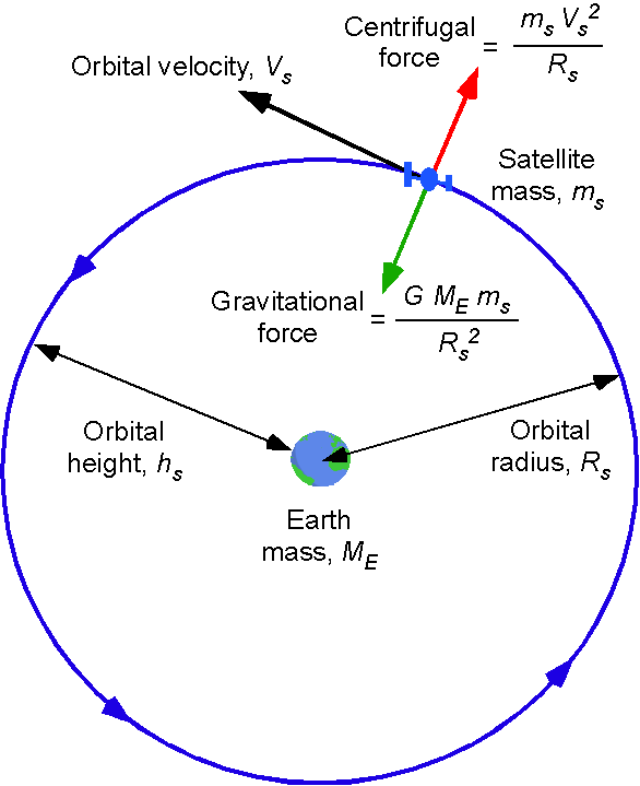
The force equilibrium of a satellite of mass  is
is
(9) 
where  is the tangential or orbital speed of the satellite, and
  is the radius of its orbit as measured from the center of the Earth. Solving for gives
(10) 
so the orbital speed is inversely proportional to the square root of its orbital radius. Notice that this prior result does not depend on the satellite’s mass.
It can be concluded from Eq. 10 that satellites that orbit closer to Earth (i.e., the value of is less) experience more substantial effects of gravity, as shown in the figure below. Therefore, they must travel faster than a satellite orbiting farther from Earth to stay in orbit. In a geosynchronous orbit (GEOS), the satellite takes 24 hours to complete one orbit around the Earth, so it appears stationary in the sky relative to an observer on the Earth. This behavior is helpful for communication satellites that need to remain over a specific location on the Earth’s surface. The altitude of GEOS is high enough at 35,406 km (22,000 miles or about three Earth diameters) above the surface that the satellite is not affected by the drag from the Earth’s atmosphere, which would cause its orbit to decay. Note: Satellites at that altitude with no orbital tilt (0 degrees) are called geostationary, and those that have an inclination other than zero are called geosynchronous.
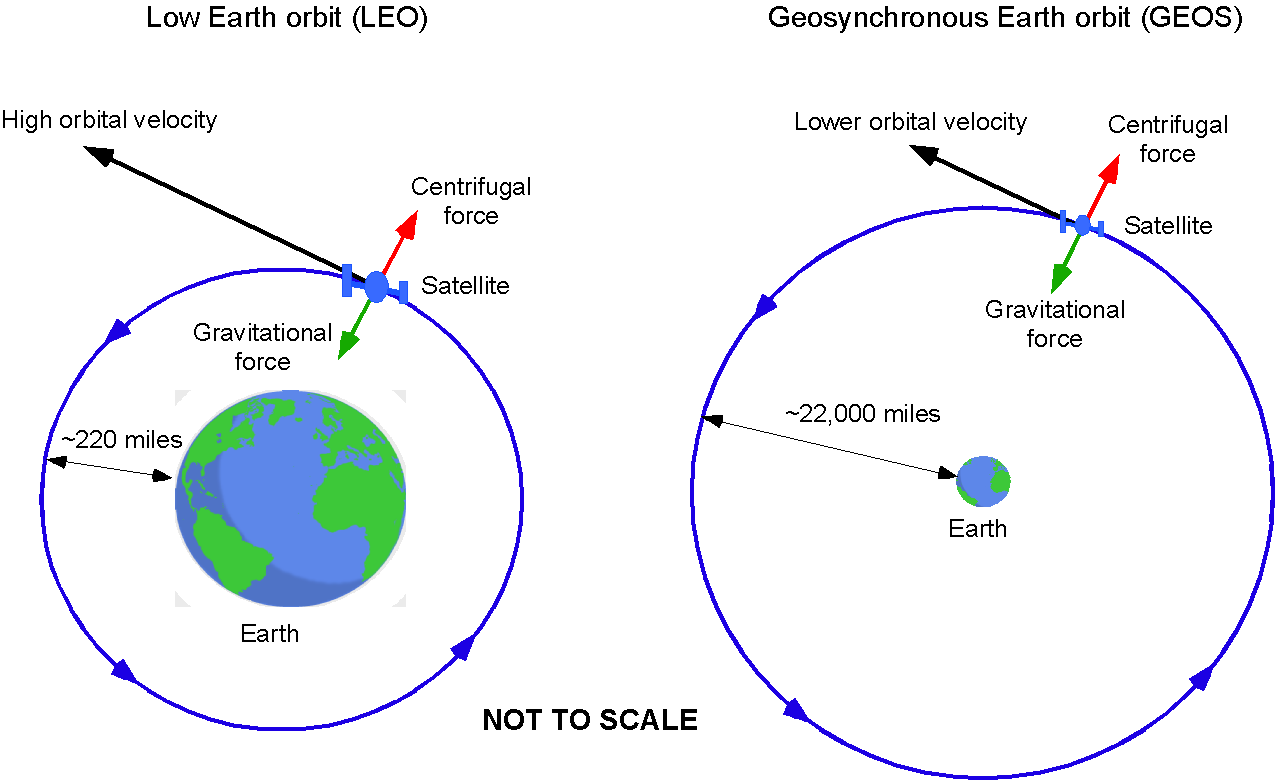
Low Earth orbit (LEO) is much closer to the Earth’s surface. Satellites in LEO are subject to drag from the Earth’s atmosphere, which requires more energy to maintain the orbit and also limits the lifespan of such satellites. For example, the International Space Station is in LEO at only about 402 km (250 miles) above the surface of the Earth. It must travel at about 27,600 kph (7.67 km/sec or 17,150 mph) to stay in orbit! Many satellites, however, orbit in GEOS at a height of more than 35,406 km (22,000 miles) above the surface, and so only (!) have to travel at about 10,783 kph, 3 km/sec or 6,700 mph) to maintain their orbits.
Check Your Understanding #2 – Height of a geosynchronous orbit
How high above the surface of the Earth is a satellite in a geosynchronous orbit? Assume a circular orbit. Assume also that = 398,600.5 km s, the angular velocity of the Earth,
  , is
, is  rad s
rad s , and the radius of the Earth, , is 6,378.1 km.
Show solution/hide solution.
A geosynchronous orbit is one in which the satellite maintains its position (approximately) over a point on the surface of the Earth. To maintain such a position, the angular velocity of the satellite,  , about the Earth must match the Earth’s angular velocity, . We know that
![\[ V_s = \sqrt{ \frac{\mu_E}{R_s} } \]](https://eaglepubs.erau.edu/app/uploads/quicklatex/quicklatex.com-66e62bd42d8b5b0c50724d07053a2c75_l3.svg "Rendered by QuickLaTeX.com")
where is the radius of the satellite’s orbit relative to the Earth’s center. Also, from simple physics
![\[ V_s = \omega_s R_s \]](https://eaglepubs.erau.edu/app/uploads/quicklatex/quicklatex.com-30fc9af6daf202d1d1ed1ab059fe0170_l3.svg "Rendered by QuickLaTeX.com")
Equating these two latter equations gives
![\[ \omega_s R_s = \sqrt{ \frac{\mu}{R_s} } \]](https://eaglepubs.erau.edu/app/uploads/quicklatex/quicklatex.com-56fb6b8809f488747107314e5ce50676_l3.svg "Rendered by QuickLaTeX.com")
Solving for the orbital radius, , gives
![\[ R_s = \left( \frac{\mu}{{\omega_s}^2} \right)^{1/3} \]](https://eaglepubs.erau.edu/app/uploads/quicklatex/quicklatex.com-2b42aa9514a248e665adf695a0a85691_l3.svg "Rendered by QuickLaTeX.com")
We know that = 398,600.5 km s = 3.985  m s. Also, based on the known angular rotational speed of the Earth and its average radius, then
  rad s. Therefore, calculating gives
![\[ R_s = \left( \frac{\mu_E}{{\omega_E}^2} \right)^{1/3} = \left( \frac{3.985 \times 10^{14}}{(7.29 \times 10^{-5})^2} \right)^{1/3} = 42,168.8~\mbox{km} \]](https://eaglepubs.erau.edu/app/uploads/quicklatex/quicklatex.com-3a60babe8c980ac8327e303cb860f4d4_l3.svg "Rendered by QuickLaTeX.com")
This result means that a satellite in geosynchronous orbit will be at the height of  above the surface of the Earth, where for the Earth is 6,378.1 km. Therefore, satellites must be placed at about 35,790.7 km (22,236 miles) above the surface.
Orbit Equation
The orbit equation explains the orbital motion of a lesser mass about a higher total mass at rest. It is often referred to as a solution to the two-body problem. After a mass or payload, e.g., a satellite, is in orbit, the principles of orbital mechanics govern its motion and position. Orbital mechanics studies the motions of planets, satellites, and space vehicles moving under the influence of gravity, their own thrust, etc. The study of orbital mechanics helps engineers plan and execute missions to explore the solar system and to deploy and control satellites for various purposes, including communication, navigation, weather prediction, and Earth observation.
Energy Equation
After launch, a satellite will have some initial velocity, momentum, and total energy. The launch vehicle has imparted this energy up through the point of final burnout. It has two parts: kinetic energy, which is associated with its motion, and gravitational potential energy, which is associated with its altitude or height. The balance between these two forms of energy determines the satellite’s motion. As the satellite moves along its orbit, the gravitational potential energy changes because of the decrease in altitude, and this energy is transformed into kinetic energy.
This balance between gravitational potential energy and kinetic energy allows the satellite to remain in orbit. The Earth’s gravitational attraction keeps the satellite moving in its path, while its velocity and momentum prevent it from falling to Earth. Other factors, such as atmospheric drag, solar radiation pressure, and gravitational perturbations from other celestial bodies, also affect the stability of the satellite’s orbit.
For circular orbits, the gravitational potential energy, which is usually given the symbol  , of a satellite of mass that orbits around a central mass
  , is
, is
(11) 
which is obtained by using the universal law of gravitation.
This latter result is easily proved by determining the work needed to raise a mass from one altitude,  , to another altitude,
  . The total work to do this can be written as
(12) 
Evaluating the integral gives
(13) 
In orbital mechanics, the reference point for evaluating the potential energy is assumed to be at infinity, i.e.,  . In this case then
  (energy is conserved) so
(14) 
or in general
(15)
Notice that because the reference for the potential energy is set to infinity, the potential energy is negative if the satellite is bound in an orbit around Earth or another planet. Therefore, the closer the two masses are, the stronger the gravitational potential energy of the satellite and the more negative the value of .
The kinetic energy, which is given the symbol  , is best expressed in terms of polar coordinates, i.e.,
(16) 
which can be rationalized from the schematic shown below.
Because  (i.e., solid body rotation), then this latter equation can be written as
(17) 
Therefore, the total energy is
(18) 
In the case of a satellite of mass orbiting the planet Earth, then
(19) 
Equation of Motion of a Satellite (Two-Body Problem)
Recall that the energy equation is
(20) 
where the satellite has a mass . Expanding out, then
(21) 
noting that this latter equation involves both  and
and  , i.e., it has two degrees of freedom.
Start first with the coordinate. In this case
(22) 
implying that  is constant, which is the angular momentum of the satellite about the central mass. This means that angular momentum is conserved, i.e.,
(23) 
assuming, of course, no thrust is applied to the satellite. This latter equation is often written in terms of “per unit mass,” so the momentum per unit mass is
(24) 
Leaving out all the detailed steps of the derivation, which can be found in any textbook on orbital mechanics, it can be shown that the equation of motion in the direction is
(25) 
where
(26) 
It can be further shown that the solution to this equation for a given value of is
(27) 
where  , , and
  are constants. The angle is measured between the vector and the axis of periapsis, also called the true anomaly. This preceding algebraic equation describes the orbital trajectory of the satellite of mass around another larger mass and is usually referred to as the orbit equation.
Solutions to the Orbit Equation
In canonical form, these solutions to the orbit equation are often written in polar coordinates as
(28) 
where  is called the parameter of the orbit and
  is called the eccentricity of the orbit.
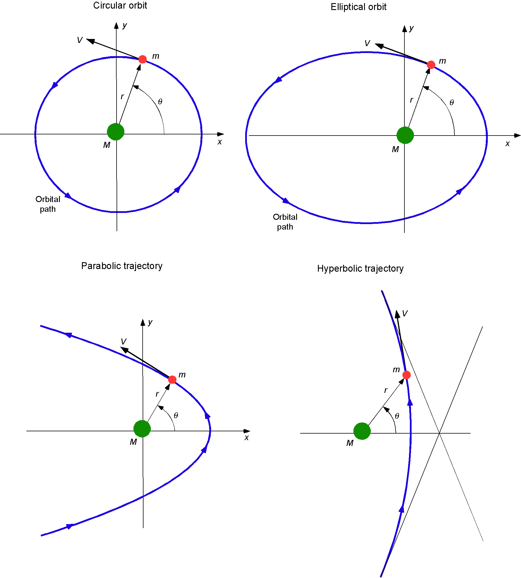
This preceding solution is one of the most fundamental equations in all orbital mechanics and gives several different orbital trajectories, called conic sections or conics. As shown in the figure below, four orbital trajectories can be derived from the orbit equation, depending on the value of , these being:
-
-
-
-
 , the orbit is circular.
 , the orbit is elliptical.
 , the orbit is parabolic.
 , the orbit is hyperbolic.
-
-
-
Kepler’s Laws of Orbital Motion
Johannes Kepler concluded that the planets in the solar system moved around the Sun in elliptical orbits. Using the meticulous astronomical measurements compiled by his mentor, Tycho Brahe, Kepler made the following conclusions:
- All planets move in elliptical orbits with the Sun at one focus.
- A line joining any planet to the Sun sweeps out equal areas in equal times.
- The square of the period of any planet about the Sun is proportional to the cube of the planet’s mean distance from the Sun.
Kepler then developed his three foundational principles of orbital mechanics, which, in their general form, apply to any mass that is orbiting about another, larger, central mass. These are now known as Kepler’s Laws of Orbital Motion. At the time of their formulation, they were considered to be exact laws, and over the centuries, they have been found to give very close approximations to actual planetary motions.
Kepler’s laws can also be deduced from Newton’s laws of motion and the law of universal gravitation, although the formal annunciation of Newton’s laws came about nearly a century later. Indeed, many scientists have pointed out that Isaac Newton referred to Johannes Kepler’s work in the traditional formulation of his gravitational theory in the publication of his Principia. Newton was to show that Kepler’s laws are a particular case of the gravitational motion of  bodies where all the bodies may be treated as point masses. Their motion is not affected by each other except for the gravitational attraction of a large central mass. Therefore, Kepler’s laws are solutions to the so-called two-body problem.
Kepler’s 1st Law
Kepler’s first principle (or law) was developed from his observations that the planets’ orbital trajectories are ellipses about the Sun with the Sun at the focus: “A satellite describes an elliptical orbit around its center of attraction.” The figure below shows an annotated elliptical orbit with semi-major length  and semi-minor length
  .
.
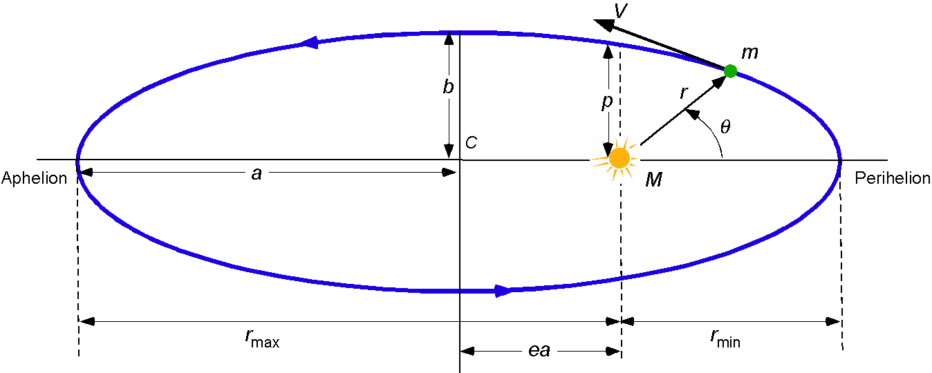
This first law permits two conclusions to be drawn about how it applies to planets or satellites in orbit about another planet or body:
- Because they move in a curvilinear path, an external force—the force of gravitational attraction—acts upon them.
- They will have constant momentum and energy when they move in an orbit.
Notice that the value of is known as the true anomaly, which is the angle between the perigee and the position vector to the orbiting mass or satellite. If the semi-major axis and eccentricity for an orbit are known, then at perigee or a true anomaly  , then
(29) 
At apogee, or a true anomaly of  , then
(30) 
Kepler’s 2nd Law
By studying the orbit of Mars, Kepler noticed that a line drawn between the center of the Earth and that of Mars swept out an equal area in an equal amount of time, as illustrated in the figure below. He reasoned that when the planet is closest to the Sun, or at perihelion, it must travel faster than when further from the Sun at its aphelion. This observation became the basis for Kepler’s second law or “law of areas,” i.e., “A satellite sweeps out equal areas in equal times around their center of attraction.”
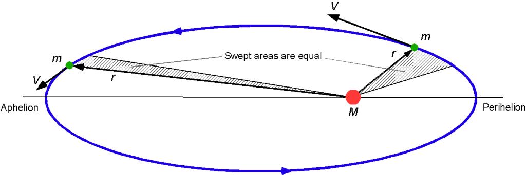
Notice that the areas of the small shaded areas can be written as
(31) 
where  is the angular distance. The angular momentum of a satellite is conserved, i.e.,
(32) 
so for a constant mass, , then  constant. The change in swept area with respect to time is
(33) 
which confirms Kepler’s second law.
Kepler’s second law also permits two conclusions to be drawn about how it applies to planets or satellites in orbit about another planet or body:
- Planets do not move with constant speed along their orbits.
- A planet moves fastest at perihelion (or perigee) and slowest at its aphelion (or apogee).
Kepler’s 3rd Law
Kepler’s third law, established much later than the first two laws, states: “The square of the orbital period is directly proportional to the cube of the average distance between the satellite and the center of attraction.” The third law appeared in what Kepler called his opus magnum, namely the book “Ioannis Keppleri Harmonices mundi libri V,” or in English “The Five Books of Johannes Kepler’s The Harmony of the World,” which was published in 1619. More precisely, his third law quantifies that the orbital period,  , is proportional to the cube of the semi-major length, , of the elliptical orbit, i.e.,
(34) 
or
(35) 
Kepler’s third law, often called the “harmonic law,” also verifies that the larger the orbit, the longer it takes for the satellite to traverse it.
Kepler’s third law can also be derived from Newton’s universal law of gravitation, i.e., by using
(36)
Consider a satellite of mass traveling at a velocity  in a circular orbit of radius about a central mass . The force equilibrium is that the outward inward centrifugal force equals the gravitational attraction, i.e.,
(37) 
The satellite will travel a distance of  in one orbital period , so is
(38) 
Therefore,
(39) 
which, on rearrangement, gives
(40) 
noticing that this latter result does not depend on the satellite’s mass. The conclusion is that
(41) 
which is Kepler’s third law.
Kepler’s third law allows predictions of the orbit of any satellite or object in space traveling around a central body. While it has been previously derived by assuming a circular orbit, it also applies to an elliptical orbit. This relationship can be more formally quantified by
(42) 
where
(43)
and where is the length of the semi-major axis of the satellite’s elliptical orbit.
Now consider the case of the orbital mass of one satellite about a large central mass with period  and semi-major axis length
  , and let be the mass of another satellite about with period
  and semi-major axis length
  . Then the use of Eq. 42 gives
(44) 
and
(45) 
(46) 
which is the correct form of Kepler’s third law.
However, because and are generally much smaller than , even for the most massive planets that orbit the Sun, such as Jupiter, then the quantity on the left side of Eq. 46 is almost unity, i.e.,
(47) 
so that
(48) 
which is the most commonly used form of Kepler’s third law.
Check Your Understanding #3 – Orbit time of Mars?
The Earth orbits around the Sun in one year, i.e.,  365.256 days. (Note: Ever wonder why we have a leap year every four years?) The length of the semi-major axis of the Earth’s orbit is
  km. Now, if the semi-major axis,
  , of Mars, is
  km, then what will the orbit time,
  , of Mars be?
Show solution/hide solution.
Using Kepler’s third law, then
![\[ T = 2 \pi \sqrt{ \frac{a^3}{\mu}} \approx 2 \pi \sqrt{ \frac{a^3}{G \, M}} \]](https://eaglepubs.erau.edu/app/uploads/quicklatex/quicklatex.com-cd9ab22ae9a98e5eb80a1f9f6b717061_l3.svg "Rendered by QuickLaTeX.com")
Both the Earth and Mars orbit around the Sun, so the value of  is the same for both planets, so that
![\[ \frac{T_M}{T_E} = \sqrt{ \frac{{a_M}^3}{{a_E}^3} } = \left( \frac{a_M}{a_E} \right)^{3/2} \]](https://eaglepubs.erau.edu/app/uploads/quicklatex/quicklatex.com-5bb8c90e433b484ba45d8853424d1e70_l3.svg "Rendered by QuickLaTeX.com")
Inserting the numerical values gives
![\[ T_M = T_E \left( \frac{a_M}{a_E} \right)^{3/2} = \left( \frac{2.278}{1.495} \right)^{3/2} = 696.96~\mbox{days} = 1.88~\mbox{years} \]](https://eaglepubs.erau.edu/app/uploads/quicklatex/quicklatex.com-5f62c5c64c58a69689a951bd537bdbcf_l3.svg "Rendered by QuickLaTeX.com")
Determining the Mass of a Planet
One of the questions people often ask is how the mass of a planet is determined. However, any planet with a satellite orbiting around it, either natural or artificial, can be used to measure the planet’s mass by studying the satellite’s orbital motion and using Kepler’s third law.
Consider first the orbit of the Earth around the Sun, the Sun having mass  and the Earth having mass with orbital semi-major axis length
  . Then using Eq. 44 gives
(49) 
Consider next a satellite of mass in orbit around the Earth with a period  and orbital semi-major axis length
  . In this case, then
(50) 
Therefore, using both of these prior equations, then
(51) 
The quantities , ,  , and , on the right-hand side of Eq. 51 can all be measured, so the Earth’s mass relative to the Sun can then be determined. It turns out that the Earth’s mass is approximately 333,000 times less than the mass of the Sun. As a reference, the Sun’s mass is estimated to be roughly
  kg.
kg.
The uncertainty in the measurement value of the Earth’s mass is also related to the uncertainty in estimating the gravitational constant, . Modern measurements of have been repetitions of the classic Cavendish experiment, reducing the uncertainty in measuring the Earth’s mass. It is generally accepted that the Earth’s mass, , is  kg. The Earth’s mass is also somewhat variable, depending on the relative balance of the accretion of inward-falling material, including micrometeorites and cosmic dust, and the loss of atmospheric gasses.
Check Your Understanding #4 – Calculating the mass of Mars
The Viking Mars orbiter probe was placed in a circular orbit 17,000 km above the Martian surface. Doppler measurements of the transmitted signals from the probe indicated that it was at an orbital velocity,  , of 1.46 km/s. Calculate the mass of Mars,
  , in terms of the mass of the Sun, , given that the diameter of Mars,
  , is 6,770 km and the radius of the Mars orbit about the Sun, , is 1.524 AU. Note: 1 AU =
  km; 1 year =
  s.
s.
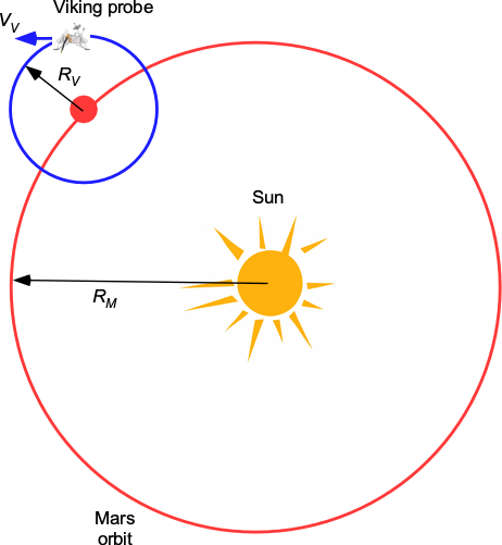
Show solution/hide solution.
For the Sun and Mars, using Kepler’s third law gives
![\[ T_M = a_M \,^{3/2} = 1.524\,^{3/2} = 1.88~\mbox{years} \]](https://eaglepubs.erau.edu/app/uploads/quicklatex/quicklatex.com-bf804ba319139555a16387080cfe4c74_l3.svg "Rendered by QuickLaTeX.com")
For Mars and the Viking probe, then
![\[ a_V = 17,000 + \frac{d_M}{2} = 17,000 + \frac{6,770}{2} = 20,384~\mbox{km} = 1,3635 \times 10^{-4}~\mbox{AU} \]](https://eaglepubs.erau.edu/app/uploads/quicklatex/quicklatex.com-092d58bed9a87e401d273da23c89a09b_l3.svg "Rendered by QuickLaTeX.com")
Therefore, the time for Viking to orbit Mars,  , will be
![\[ T_V = \frac{2 \pi \, a_v}{V_V} = \frac{2 \pi \times 20,385}{1.46} = 2.7797 \times 10^{-3}~\mbox{years} = 87,727.9~\mbox{s} \]](https://eaglepubs.erau.edu/app/uploads/quicklatex/quicklatex.com-a1fee90327acd7c5faf5320e91013132_l3.svg "Rendered by QuickLaTeX.com")
We also know that
![\[ \left( \frac{T_M}{T_V} \right) = \left( \frac{a_M}{a_V} \right)^3 \left( \frac{M_S + M_V}{M_S + M_M} \right) = \left( \frac{a_M}{a_V} \right)^3 \left( \frac{M_M}{M_S} \right) \]](https://eaglepubs.erau.edu/app/uploads/quicklatex/quicklatex.com-06449ee3597a4470880b7eff98e3ba88_l3.svg "Rendered by QuickLaTeX.com")
Rearranging gives
![\[ \frac{M_M}{M_S} = \left( \frac{T_M}{T_V} \right)^2 \left( \frac{a_V}{a_M} \right)^3 = \left(\frac{1.88}{2.7797 \times 10^{-3} } \right)^2 \left( \frac{1.3635 \times 10^{-4}}{2.524} \right)^3 \]](https://eaglepubs.erau.edu/app/uploads/quicklatex/quicklatex.com-bf4ad300b653ae8760be95524ecfe3d4_l3.svg "Rendered by QuickLaTeX.com")
Therefore,
![\[ \frac{M_M}{M_S} = 3.281 \times 10^{-7} \]](https://eaglepubs.erau.edu/app/uploads/quicklatex/quicklatex.com-8db0ecc6559cc3f41c15f89dae5d4659_l3.svg "Rendered by QuickLaTeX.com")
and
![\[ M_M = 3.2811 \times 10^{-7} \, M_S \]](https://eaglepubs.erau.edu/app/uploads/quicklatex/quicklatex.com-9f7905cd8cb3777fe068d4a90425f212_l3.svg "Rendered by QuickLaTeX.com")
So, the mass of Mars is about 3,047,760 times less than that of the Sun.
How long does it take the Moon to go around Earth?
It takes 27 days, 7 hours, 43 minutes, and 11.461 seconds for the Moon to complete one full orbit around the Earth. This period is called the sidereal month. However, the Moon takes about 29.5 days to complete one cycle of phases, called the synodic month. The difference between the sidereal and synodic months is that as the Moon orbits around the Earth, the Earth also orbits around the Sun. Therefore, the Moon must travel farther in its orbit to catch up and compensate for the added distance to complete the rotational phase cycle.
Orbital Energy
Orbital mechanics is mainly governed by the energy of the orbiting satellite, consisting of kinetic and potential energy. The total mechanical energy of an object in orbit around another mass must remain constant as a result of the conservation of energy. In addition to energy, the laws of orbital mechanics are also influenced by the law of universal gravitation, which describes the attractive force between two masses, and the laws of motion, which relate how an object moves in response to forces acting on it. These fundamental laws help explain satellites’ motion and other characteristics in orbit around Earth or other celestial bodies.
Circular Orbits
The kinetic energy of the satellite, , is
(52) 
and the associated potential energy, , is
(53) 
Therefore, the total energy is
(54) 
The force equilibrium for a satellite of mass in a circular orbit is
(55) 
where is the tangential or orbital speed of the satellite, and is the radius of its orbit as measured from the center of mass, . Rearranging the preceding equation gives
(56) 
and so the energy equation becomes
(57) 
(58) 
which says that the energy of the satellite in orbit around the mass is negative. This result can also be proven for an elliptical orbit.
Negative Potential Energy?
What does it mean when the energy given by Eq. 58 is negative? This situation is called a bound orbit, in that the satellite is bound to a mass or planet, i.e., it is gravitationally bound in the same manner that the Earth is bound to the Sun and the Moon is bound to the Earth. A bound orbit is a closed orbit, either circular or elliptical, and the body or satellite will remain around the source of the gravitational attraction. Circular orbits have the minimum energy. Bound circular and elliptical orbits always have  . Unbound trajectories, such as parabolic orbits and hyperbolic orbits, will have
  , and the object will escape from the source of the gravitational attraction.
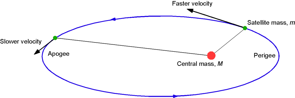
Elliptical Orbits
It will be apparent that when a satellite follows an elliptical rather than a circular orbit, its total energy  is also conserved. However, in a non-circular orbit, there must always be an interchange between a satellite’s kinetic energy, , and its potential energy, . This latter result is a direct outcome of Kepler’s second law: a satellite will speed up when it is closer to the central mass at its perigee and slow down when it is further away at its apogee, as shown in the figure below.
The energy equation for a satellite of mass in an elliptical orbit with a semi-major axis length about a central mass can be written as the sum of its kinetic energy and the potential energy, i.e.,
(59) 
The total kinetic energy can be written as
(60) 
and the total mechanical energy becomes
(61) 
The energy can also be written as
(62) 
where
(63) 
The energy is usually written per unit mass of the satellite, i.e.,
(64) 
Because the orbital energy is constant, the overall size of the orbit remains constant. Therefore, a conclusion is that the satellite will move the fastest at its closest point to the central mass , i.e., at its perigee (or perihelion) where  and slowest at its farthest point, i.e., at its apogee (or aphelion) where
  . It can be shown the velocity, , of a satellite in an elliptical orbit where is the distance between the satellite and central mass by
(65) 
which is historically called the vis-viva equation. Therefore, at perihelion, its velocity is
(66) 
and at aphelion, its velocity is
(67) 
The eccentric anomaly, , is another angular parameter that defines the position of a body moving along an elliptic orbit. Indeed, the eccentric anomaly is one of three angular parameters (“anomalies”) that define a position along an orbit, the other two being the true anomaly, as previously mentioned, and the mean anomaly, . The eccentric anomaly is related to the mean anomaly by Kepler’s equation, i.e.,
(68) 
which is a transcendental equation. The symbol conflict with mass should be noted. Given and in Kepler’s equation, it is trivial to find . However, if and are known, then must be determined numerically using an interactive approach.
Check Your Understanding #5 – Orbital motion of a comet
A comet moves in an elliptical orbit about the Sun such that its orbit is coplanar with the orbit of the Earth. The comet is observed to cross the Earth’s orbit at a time where its heliocentric velocity is 31.0 km/s, and its true anomaly is 140 . Taking the Earth’s orbit to be circular, calculate the semi-major axis length and eccentricity of the comet’s orbit and the time before the comet next crosses the Earth’s orbit.
Show solution/hide solution.
At time  then = 1.0 AU,
  = 140, and = 31.0 km/s = 6.544 AU/year. Using the vis-viva equation for a body in an elliptical orbit, then
![\[ V = \sqrt{ \mu \left( \frac{2}{r} - \frac{1}{a} \right)} \]](https://eaglepubs.erau.edu/app/uploads/quicklatex/quicklatex.com-f888e640848af961ab2d7c10f9b7b15c_l3.svg "Rendered by QuickLaTeX.com")
In this case, = 1 AU, so
![\[ \left( \frac{2}{r} - \frac{1}{a} \right) = \frac{V^2}{\mu} = \frac{6.544^2}{4 \pi^2} = 1.0848 \]](https://eaglepubs.erau.edu/app/uploads/quicklatex/quicklatex.com-c31ec9060bde1c24ee5870635e9056bf_l3.svg "Rendered by QuickLaTeX.com")
Therefore,
![\[ \frac{1}{a} = 2.0 - 1.0848 = 0.915 \]](https://eaglepubs.erau.edu/app/uploads/quicklatex/quicklatex.com-eff5ef4fac42a2df2f934119d9a92e98_l3.svg "Rendered by QuickLaTeX.com")
So, the semi-major length of the orbital axis is  . We also know that for an elliptical orbit, then
![\[ r = \frac{a(1 - e^2}{1 + e \cos f} \]](https://eaglepubs.erau.edu/app/uploads/quicklatex/quicklatex.com-c2b940c7f84474e1840b6bad7714a3c9_l3.svg "Rendered by QuickLaTeX.com")
which on rearrangement leads to a quadratic in , i.e.,
![\[ a e^2 + \cos f e + (1 - a) = 0 \]](https://eaglepubs.erau.edu/app/uploads/quicklatex/quicklatex.com-bb0ac002825313ea46176a5169b89125_l3.svg "Rendered by QuickLaTeX.com")
The solution for the eccentricity is = 0.80625, which is a very stretched elliptical orbit. Because
![\[ r = a ( 1 - e \cos E) \]](https://eaglepubs.erau.edu/app/uploads/quicklatex/quicklatex.com-38d76c0896b868a3049267fcbabc466e_l3.svg "Rendered by QuickLaTeX.com")
where is the eccentric anomaly, then
![\[ \left( 1 - \frac{r}{a} \right) \frac{1}{e} = \cos E = \left( 1 - \frac{1}{1.093} \right) \frac{1}{0.8063} = 0.1052 \]](https://eaglepubs.erau.edu/app/uploads/quicklatex/quicklatex.com-31b934fa6e4fcad9a6e096628f82f3cf_l3.svg "Rendered by QuickLaTeX.com")
so that  at orbit crossing. The period of the comet’s orbit (paying attention to the units) is
![\[ \tau = 2 \pi \sqrt{ \frac{a^3}{\mu} } = \sqrt{ a^3} = \sqrt{ 1.093^3} = 1.142~\mbox{years} \]](https://eaglepubs.erau.edu/app/uploads/quicklatex/quicklatex.com-06205a34b06995a83d54aa794b06ea1b_l3.svg "Rendered by QuickLaTeX.com")
At = 140 then is 83.96 = 1.465 radians, which using Kepler’s equation means that
![\[ M = E - e \sin E \]](https://eaglepubs.erau.edu/app/uploads/quicklatex/quicklatex.com-594ca572d1e720292cd89fd331b0a60e_l3.svg "Rendered by QuickLaTeX.com")
where is the mean anomaly, and so = 0.6636 in this case. Also, the mean angular velocity (orbit frequency) is
![\[ n = \frac{2 \pi}{T} = \frac{2 \pi}{1.142} = 5.501~\mbox{rads/year} \]](https://eaglepubs.erau.edu/app/uploads/quicklatex/quicklatex.com-672203e884fca75d1a96a280e92b433e_l3.svg "Rendered by QuickLaTeX.com")
Therefore, the orbit time is
![\[ t_1 = \frac{M}{n} = \frac{0.6636}{5.501} = 0.1206~\mbox{years} \]](https://eaglepubs.erau.edu/app/uploads/quicklatex/quicklatex.com-cae85768ece3298b7445523fd973c0ff_l3.svg "Rendered by QuickLaTeX.com")
At = 220 and = 276.04, then now
![\[ m = E - e \sin E = 4.818 - 0.80625 \sin 4.818 = 5.6196 \]](https://eaglepubs.erau.edu/app/uploads/quicklatex/quicklatex.com-f46886e0d86c1c5b5e5ce19b37caaac0_l3.svg "Rendered by QuickLaTeX.com")
Therefore,
![\[ t_2 = \frac{M}{n} = \frac{5.6196}{5.501} = 1.0216~\mbox{years} \]](https://eaglepubs.erau.edu/app/uploads/quicklatex/quicklatex.com-f05babad6f61080c33de8ac84b4ee7e0_l3.svg "Rendered by QuickLaTeX.com")
and so the time to wait for the next orbit crossing of the comet will be
![\[ t_2 - t_1 = 1.0216 - 0.1207 = 0.901~\mbox{years} \]](https://eaglepubs.erau.edu/app/uploads/quicklatex/quicklatex.com-d529cda78957964adbfcd9d30b01dd57_l3.svg "Rendered by QuickLaTeX.com")
Energy Considerations of Changing Orbits
It is often required that a satellite or other spacecraft be able to change its orbit from a lower to a higher orbit or vice versa, as shown in the example below. After launch, a satellite may be parked in an initial (lower) orbit until the orbit stabilizes, then is boosted to its final altitude. Raising the orbital altitude requires energy and propellant. A rocket engine must be fired to create work,  , to increase the radius of the orbit from
  , where it has energy
  , to a radius
  , where it has energy
  . Often, the orbital altitude relative to the surface of the Earth, , is used such that
  and
and  , where is the radius of the Earth.
Consider a satellite or spacecraft of mass in an initially circular orbit of radius about the Earth, which has mass . Its orbital energy is
(69) 
To get to the higher orbit, the conservation of energy requires
(70) 
where is the work required to raise the orbital altitude. Inserting the values of and gives
(71) 
Therefore, the work (or energy) needed to raise the orbit is
(72) 
and further rearranging gives
(73) 
Finally, in terms of orbital altitude, then
(74) 
Similar principles can be applied regarding elliptical orbits.
Hohmann Transfer Orbit
The Hohmann cotangential elliptic transfer orbit is a minimum-energy orbital maneuver used to transfer a spacecraft between two orbits at different altitudes, as shown in the diagram below. The maneuver is accomplished by placing the spacecraft into an elliptical transfer orbit, called a Hohmann transfer orbit, where the perigee and apogee of this trajectory are tangential to the initial and target orbits. The procedure is named after Walter Hohmann, whose early work on space flight and rocket science helped lay down the foundations of astrodynamics.
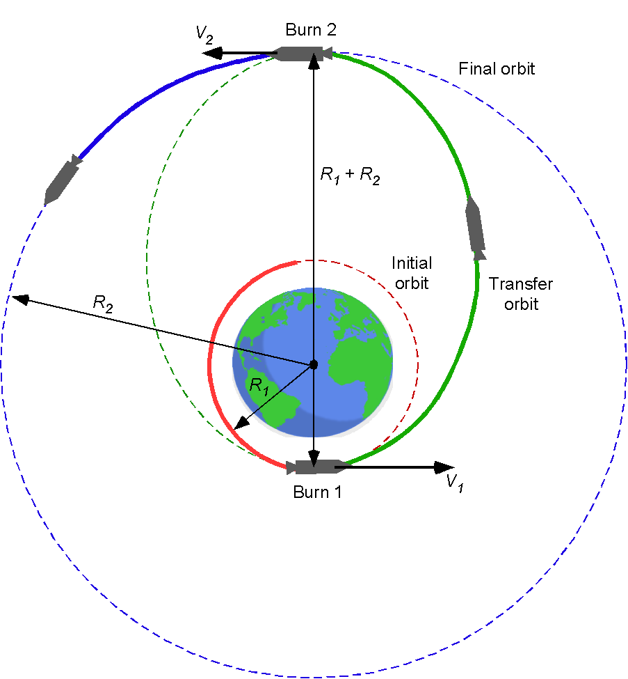
The transfer maneuver needs excess energy, so the spacecraft uses two impulsive engine burns. The first burn is required to increase  , break out of the initial circular orbit, and establish the elliptical transfer orbit. The second burn obtains the spacecraft’s velocity needed at the altitude of the final (target) orbit,
  .
.
Notice that a second burn is needed because the spacecraft loses its kinetic energy as it reaches the aphelion of the transfer orbit, so it will be too slow to stay at the final orbital altitude without the  boost obtained using the second burn to circularize the orbit. Depending on the spacecraft’s orientation when it reaches the target orbit, it may need to be reoriented so that the engine(s) can fire in the orbital direction to speed it up.
Assuming a transfer orbit around the Earth, for the lower (initial) orbit, solving for gives
(75) 
and for the higher (final) orbit, then
(76) 
Remember that in the higher, final orbit will be lower than in the lower, initial orbit. However, at the end of the transfer orbit, the spacecraft’s velocity will still be less than the needed without a burn.
The total energy of the spacecraft in the initial orbit, , is
(77)
and in the final orbit, it must be
(78) 
In the Hohmann elliptical transfer orbit, the energy  will be
(79) 
noticing that the length of the semi-major axis of the elliptical transfer orbit is
(80) 
Consider the point in time just after the first burn to leave the initial orbit, in which a change in velocity,  , is required. In this case, the total energy just after the burn can be written as
(81) 
where  is the velocity immediately after the burn, i.e., at the perigee of the elliptical transfer orbit. Notice that the mass of the spacecraft, , cancels out in this latter equation so that
(82) 
Solving for gives
(83) 
(84) 
After the spacecraft is established in the transfer orbit, it will continue under gravity until it reaches the height of the final orbit. At this point, a second burn will be needed. The velocity,  , which is at the aphelion of the transfer orbit and just before the second burn, will be
(85) 
where it will be noticed that in the first term inside the parentheses in Eq. 84 has been replaced by in Eq. 85.
However, at the end of the transfer orbit, this velocity will be too low to maintain the final orbit. Without a second burn, the spacecraft will return to the lower orbit and continue indefinitely in the transfer orbit. The velocity in the final circular orbit (Eq. 76)
must be
(86) 
so the needed  can then be calculated, i.e.
(87) 
The corresponding transfer time,  will be half of the elliptical transfer orbit time, , i.e.,
(88) 
The values of at each burn can be calculated using the rocket equation, i.e.,
(89) 
where  is the initial mass of the spacecraft at the beginning of the burn, and
  is the final (burnout) mass after the burn during which a propellant mass of
  is consumed, i.e.,
  .
.
Using the rocket equation gives
(90) 
and so
(91) 
Of course, the reverse process described can be used to decrease a spacecraft’s orbital altitude. A retro-burn will be needed at the higher orbit to reduce the velocity and start the orbital transfer. At the end of this transfer, as gravitational potential energy increases (it becomes less negative), a retro-burn will be needed to break out of the elliptical orbit and circularize it at the lower orbital altitude.
Check Your Understanding #6 – Raising an orbit using a Hohmann transfer
Calculate the two velocity increments required to change the orbit of the Viking probe from a circular orbit at 17,000 km above the Martian surface to another circular orbit of a height of 30,000 km above the surface. Assume a Hohmann cotangential elliptic transfer orbit. Also, determine the semi-major axis and eccentricity of the transfer orbit and the transfer time. The diameter of Mars, , is 6,770 km. Note: 1 AU = km; 1 year = s. Bonus: Why could the probe not be placed at an orbital altitude of 800,000 km? 
Show solution/hide solution.
Notice that in this case, is 20,385 km or 1.36354  AU and is 33,385 km or 2.2331 AU. Therefore, for the elliptical transfer orbit, the semi-major axis, , will be
![\[ a = \frac{R_1 + R_2}{2} = \frac{20,385 + 33,385}{2} = 26,885~\mbox{km} \]](https://eaglepubs.erau.edu/app/uploads/quicklatex/quicklatex.com-0f6badc2420c85e75b8a572959c8431b_l3.svg "Rendered by QuickLaTeX.com")
The corresponding eccentricity of the transfer orbit will be
![\[ e = \frac{R_2 - R_1}{R_2 + R_1} = \frac{33.385 - 20,385}{33,385 + 20,385} = 0.2418 \]](https://eaglepubs.erau.edu/app/uploads/quicklatex/quicklatex.com-7063a58f3fb3dfe4b7db9f2af00eb4ff_l3.svg "Rendered by QuickLaTeX.com")
The orbital transfer time, , will be
![\[ \tau = \pi \sqrt{ \frac{a^3}{G \, M_M} } \]](https://eaglepubs.erau.edu/app/uploads/quicklatex/quicklatex.com-068d7ee257e5870b3544c575793ab985_l3.svg "Rendered by QuickLaTeX.com")
where  in this case is for Mars. From Example #2, it was shown that
so
![\[ G \, M_M = 1.2453 \times 10^{-5} \]](https://eaglepubs.erau.edu/app/uploads/quicklatex/quicklatex.com-7e97b45e5744793fd6318078e4cb9bf9_l3.svg "Rendered by QuickLaTeX.com")
which will be in units of AU years. Therefore, the transfer time, , will be
![\[ \tau = \pi \sqrt{ \frac{a^3}{G \, M_M} } = \pi \sqrt{ \frac{(1.2453 \times 10^{-5})^3}{1.2453 \times 10^{-5}} } = 2.105 \times 10^{-3}~\mbox{years} = 18.45~\mbox{hours} \]](https://eaglepubs.erau.edu/app/uploads/quicklatex/quicklatex.com-c2e42798b4002d07633b4f3c299256d8_l3.svg "Rendered by QuickLaTeX.com")
The increments to initiate and end the the transfer will be
![\[ \Delta V_1 =\sqrt{ \frac{G \, M_M}{R_1} } = \sqrt{ \frac{1.2453 \times 10^{-5}}{1.36354\times 10^{-4}} } = 0.09133~\mbox{AU/year} = 0.167~\mbox{km/s} \]](https://eaglepubs.erau.edu/app/uploads/quicklatex/quicklatex.com-43b4cdfc6f01afb55bc026e607e076e0_l3.svg "Rendered by QuickLaTeX.com")
and
![\[ \Delta V_2 =\sqrt{ \frac{G \, M_M}{R_2} } = \sqrt{ \frac{1.2453 \times 10^{-5}}{2.2331 \times 10^{-4}} } = 0.05577~\mbox{AU/year} = 0.147~\mbox{km/s} \]](https://eaglepubs.erau.edu/app/uploads/quicklatex/quicklatex.com-6179b6b9d1cc1a7845ecb48bc5224250_l3.svg "Rendered by QuickLaTeX.com")
Bonus: At this orbital altitude, it is easily shown that the spacecraft would need a that would cause it to escape the Martian gravity and head off into space.
There is no dark side of the moon, really!
“There is no dark side of the moon, really. Matter of fact, it’s all dark. The only thing that makes it look light is the Sun.” The Moon rotates on its own axis and experiences phases of daylight and darkness, just like on Earth. However, because of the non-uniform mass distribution inside the Moon, which is like a dumbbell, it acts like a pendulum in the gravitational pull as it rotates around the Earth. Therefore, it takes the Moon the same time to turn once on its own axis as it takes to do one orbit around the Earth. This means only one side of the Moon (the nearside) is always visible from the Earth. We never see the far side of the Moon, but it is not always dark there for the same reason the nearside is not always dark – all sides are dark once a month.
Escape Velocity
How much velocity does it take to escape the Earth’s gravitational field? The escape velocity is a case where the spacecraft’s energy is high enough that an orbit is never accomplished. In other words, how fast does a spacecraft need to travel such that it continues into space and never returns to Earth under the effects of its gravitational field? The answer lies in the energy and speed given to a spacecraft.
Consider a spacecraft of mass in orbit around the Earth, as shown in the figure below. The rocket executes a burn to give it additional energy,  . Conservation of energy requires that the final energy,
  , is
, is
(92) 
Therefore, the initial energy is
(93) 
where is the radius of the initial starting orbit.
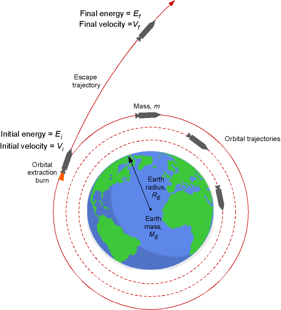
The final energy of the spacecraft is
(94) 
where is the final radius or distance from the Earth. Because  then
then
(95) 
To escape the Earth’s gravity, the spacecraft must fly far away that  . Also, suppose it is assumed that there is no excess kinetic energy at this distance. In that case, this assumption will allow an estimate of the minimum initial velocity to escape from the Earth’s gravity. The two terms on the right-hand side of the preceding equation are zero, so
(96) 
which, on rearrangement, gives
(97) 
so the minimum “escape” velocity,  , is given by
(98) 
Remember that the rocket engines must execute a burn to leave the initial orbit to obtain this velocity.
Now, armed with these results, it is possible to estimate the escape velocity for the Earth. Recall that the Earth’s mass, , is 5.97  kg, the radius of the initial orbit will be the radius of the Earth , which is 6.3781
  m, plus the orbital height, . Also, = 6.67428
  N m kg. Assuming that the orbital height relative to the radius of the Earth is small, then
(99) 
which will be the minimum velocity to escape the Earth’s gravitational field.
All spacecraft designed to travel into deep space must have a velocity larger than 11.2 km/s and will ultimately follow hyperbolic trajectories away from the Earth.
What is a Black Hole?
Everyone has heard of black holes, right? They dot the universe and are considered a region where the effects of gravity are so strong that nothing, including light, has enough energy to escape. The effect of gravity is so strong in a black hole because so much matter has been compressed into a small volume. It is not possible to see a black hole with a conventional telescope. However, the locations of black holes in the universe can be identified from the signatures of high-energy radiation and by how the stars behave differently from other stars under extremely powerful gravitational forces. An interesting image of a black hole, shown below, was taken by the Event Horizon Telescope.
By using Eq. 98 and replacing the escape velocity with the speed of light, , then
(100) 
Solving for  , which will be the radius of a black hole, gives
(101) 
which is known as the Schwarzschild equation and is named after the German astronomer Karl Schwarzschild, who calculated this exact solution for the first time.
Because the value of N m kg and the speed of light is 299,792,458 m s, then the radius of a black hole is typically small by planetary standards. For example, if the mass of a black hole were the same as the Sun ( kg), then its radius would be about 3 km, according to the Schwarzschild equation. Most black holes, however, are significantly more massive than the Sun.
Theory of General Relativity
In 1915, Einstein published his theory of general relativity. His theory, which became a paradigm shift in the physics field, showed that massive objects distort space and time, leading to a curvature in the paths of nearby objects and the phenomenon of gravitational lensing. The theory of general relativity was confirmed by the 1919 solar eclipse observation, which showed that the Sun’s gravity deflected light from stars near the Sun. Since then, the theory of general relativity has been extensively tested and verified, and has become a cornerstone principle used in modern physics. It has also provided the foundation for understanding black holes, the expanding universe, and its formation.
Einstein’s famously quoted result is
(102) 
although in Einstein’s original paper in 1905, he writes the relationship only as
(103) 
which describes the relationship between relativistic mass, , and energy, , where is the speed of light. This equation is a statement that mass is composed of energy. Relativistic mass is related to rest mass,  , using
(104) 
where  is the relative speed of the mass. In the more general case, the equation of special relativity can be written as
(105) 
where is momentum. Therefore, Eq. 105 can relate and unify the concepts of energy, momentum, and invariant mass. The values of and depend on the relative movement of the observer relative to the body. In the special case where the body is at rest, it becomes Eq. 102. Einstein’s theory of special relativity has developed into a fundamental scientific paradigm that connects mass, energy, momentum, space, and time, and today, it is accepted and used in physics, astrophysics, and cosmology.
What happens when an object approaches you at the speed of light?
Suppose an object approaches you as a stationary observer just below the speed of light. In that case, the wavelength of the light emitted from it becomes longer, effectively shifting the light toward the red end of the spectrum. This effect is known as relativistic redshift and is a consequence of the observer and the light moving relative to one another. Because of the relativistic aberration of light, objects formerly at right angles to the observer appear to shift forward. Einstein’s theory of special relativity predicts this redshift effect and is consistent with observations of high-speed astronomical objects, such as quasars and gamma-ray bursts. As the object passes you by, its light will shift into the blue end of the spectrum. Because of the aberration of light, objects formerly at right angles to the observer appear to have shifted forward. If the object travels toward you at the speed of light, the light would appear infinitely redshifted, and therefore, it would no longer be visible to you.
Mission to Mars?
Humans landed on the Moon over half a century ago but have yet to return. It is likely, however, that they will return to the Moon within this decade. However, the Moon is a long way away, about 570 km (275,000 miles), and it takes about three days to get there in a spacecraft, but at least it can be reached using conventional propulsion systems.
But what about Mars? Mars is one of Earth’s two closest planetary neighbors, Venus being the other. Mars, often called the red planet, is close enough to be seen with the naked eye on a dark night without cloud cover, looking like a bright red point of light in the sky. So if it can be seen, then surely humans should be able to go there? However, the average distance between Earth and Mars is 225,000,000 km (140,000,000 miles), about 500 times further than the Moon! Mars is also 1.5237 AUs away from the Sun, one AU (Astronomical Unit) being the average distance from the Sun to the Earth, which is km.
How does a spacecraft reach Mars, how long will it take, and how much propellant will be needed? Can astronauts even survive the long journey? How long will it take them to get back? Humans have sent probes to Mars and other planets, but can humans visit Mars or colonize it? It should be remembered that humans have yet to colonize the Moon or even Antarctica on our own planet; Mars is much more distant and hostile to humans than either of them.
Trans-Martian Injection
Some of the engineering answers to these questions can be estimated with the help of the principles previously established for a Hohmann cotangential elliptic transfer orbit, as shown in the figure below for trans-Martian injection and transit to Mars. It is assumed that the orbits of Earth and Mars are circular rather than elliptical; this assumption simplifies the mathematics considerably and gives reasonable estimates of the problem parameters.
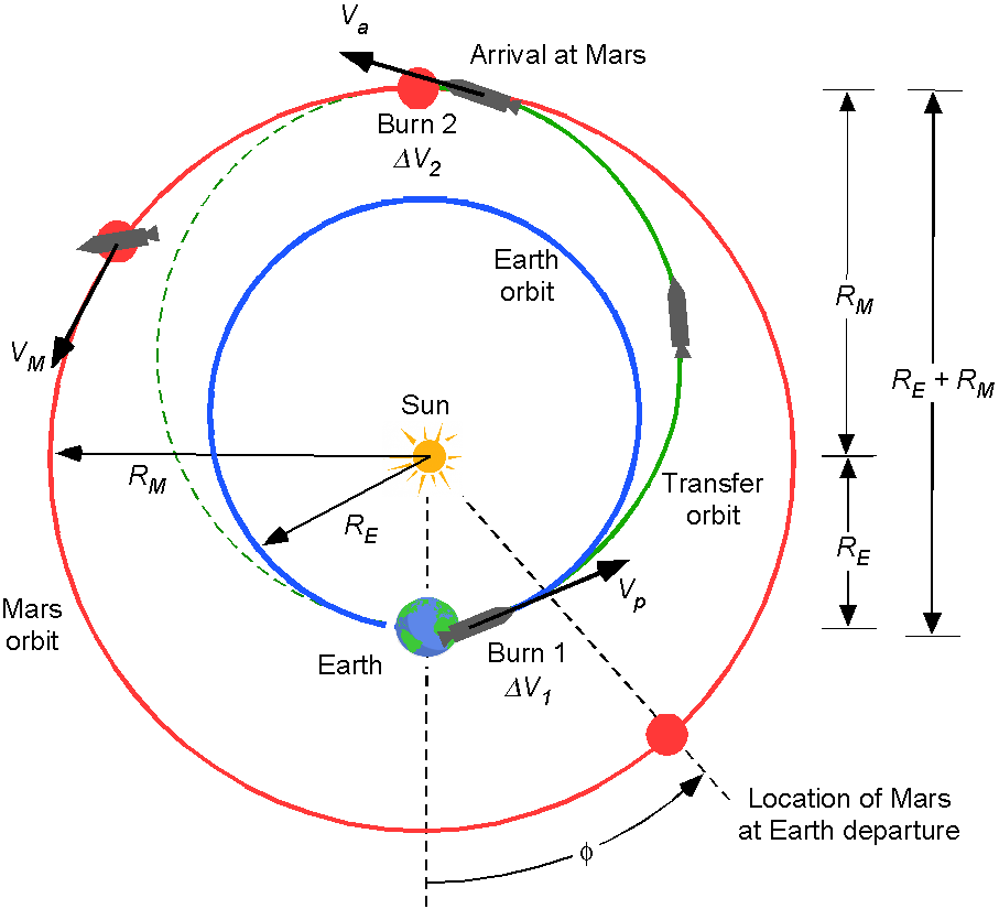
One assumption made is that the spacecraft is already in orbit around the Earth, fully fueled with propellant, and ready to make the journey to Mars. Of course, getting the spacecraft into orbit with the needed propellant is also a significant challenge. The timing of when the spacecraft sets out for Mars on the transfer orbit is critically important because they must both reach the exact orbital location simultaneously. Otherwise, the spacecraft will get there too early or too late to rendezvous with Mars. Likewise, the spacecraft’s return from Mars to Earth must be timed to allow for an Earth rendezvous, re-entry, and landing.
The time it takes to get to or from Mars can be estimated using Kepler’s third law, i.e.,
(106) 
If the period about the Sun is measured in units of years and is measured in AU units, then for Earth  and = 1, and for Mars
  . The semi-major axis length of the transfer orbit will be
(107) 
Therefore, for the transfer orbit to Mars, the orbital period is
(108) 
However, this is the time for a complete one orbit, so the transfer time to Mars will be half of this value, giving an average flight time of 0.71 years or about 8.5 months.
The exact transfer time on a mission to Mars will also depend on how close Mars and Earth are in their elliptical orbits around the Sun at any one time and the gravitational influence of other planets along the way, such as Jupiter. However, it will take much longer to get to Mars than the Moon! Even in the best scenario, a human mission to and from Mars, with just a few weeks or months spent on the surface, will likely take a couple of years. Nevertheless, this might not happen when using our conventional (chemical) propulsion systems.
Orbital Velocities
It is first necessary to calculate the orbital velocity of the Earth and Mars about the Sun. Again, circular orbits are assumed. For the Earth, its orbital velocity,  , is
, is
(109) 
where is the mass of the Sun. For Mars, its orbital velocity is  , i.e.,
(110) 
At the perigee of the transfer orbit, then
(111) 
and at the apogee of the transfer orbit
(112) 
Conservation of angular momentum of the spacecraft at the perigee and apogee of the transfer orbit gives
(113) 
(114) 
Conservation of energy for the movement about the Sun requires
(115) 
noting that cancels out on both sides of the preceding equation to give
(116) 
Using Eqs. 114 and 116 and after some algebra gives
(117) 
The for the first burn to exit the Earth’s orbit into the Hohmann transfer orbit will be
(118) 
which, after rearrangement, becomes
(119) 
For the second burn, then
(120) 
which gives
(121) 
Inserting the known values of , , etc., shows that  km/s and
  km/s.
km/s.
These values will require a significant amount of propellant, all of which has to be carried onboard the spacecraft. More propellant is needed to get the spacecraft into a Mars orbit and descend onto the surface. Staging will inevitably be required to progressively reduce the spacecraft’s mass at each phase of the flight, including a landing on Mars. However, no matter how reductions in propellant mass can be argued, getting to Mars can still be expected to require an enormous amount of propellant.
Propellant Requirements
Based on the preceding analysis, estimating the propellant mass needed to fly to Mars is possible. The mass needed depends on the type of rocket engine(s) but can be estimated from the rocket equation, i.e.,
(122) 
where  is the specific impulse for the rocket engine, is the initial mass of the spacecraft at the beginning of the burn, and is the final (burnout) mass during which a propellant mass, , is consumed, i.e., .
Using the rocket equation gives
(123) 
and so
(124)
A value for  can be assumed to make sense of this result for the Mars mission. For example, for a rocket engine using liquid hydrogen-oxygen as a propellant,
  m/s or 4.4 km/s. Hydrogen-oxygen is the most energetic chemical reaction. However, there are limits to the quantity of energy that can be extracted from chemistry, which limits what is possible with current technology and what is not.
For the first impulsive burn on a mission to Mars, then
(125) 
This means the spacecraft will consume nearly half of its initial mass,  , in propellant to get into the transfer orbit.
Consider the second burn at the end of the transfer orbit, recognizing that the initial mass has now been reduced significantly to  . In this case, the additional mass of propellant needed to circularize the orbit of the spacecraft relative to its initial mass will be
(126) ![\begin{equation*} \frac{M_P}{M_1} = 0.561 \left[ 1 - \exp \left( -\frac{2.7}{4.4} \right) \right] = 0.257 \end{equation*}](https://eaglepubs.erau.edu/app/uploads/quicklatex/quicklatex.com-946e12522932e22a2643f28b3fcb3309_l3.svg "Rendered by QuickLaTeX.com")
which is significantly less than the first burn because the spacecraft now has much less mass.
However, it becomes clear from the preceding analysis that getting to Mars will require a lot of propellant, totaling at least 75% of the spacecraft’s original mass as it sets off from the Earth. There are massive engineering implications in designing a spacecraft capable of reaching Mars, including payloads such as life-support and supplies. For example, if the spacecraft has a total mass of 50,000 kg, then about 37,500 kg of that will be the needed propellant. For a 100,000 kg spacecraft, about 75,000 kg will need to be propellant, and so on. A further amount of propellant will be required for any mid-course corrections, for a retro-burn to lower the spacecraft (or part of it) into a Mars orbit and finally descend onto the surface.
Getting Back to Earth
The astronauts have finally arrived on Mars and set up a Martian base. They collect data and do experiments. What about getting them back from Mars to Earth? Again, the propellant needed can also be estimated with some assumptions but reasonable ones. Getting back to Earth from Mars requires that the spacecraft carries the needed propellant for the return journey, which must also be part of the initial mass of the spacecraft when it leaves Earth. So, it takes propellant to transport propellant to Mars for the return mission to Earth. Now, the engineering problems are becoming more complex.
Assume that the net values of needed on the return flight are the same as on the outbound flight. On a mission to Mars, when carrying enough propellant to come back to Earth, to enter and leave the Mars orbit, then
(127) 
and to leave and re-enter Earth’s orbit
(128) 
Therefore, the propellant mass needed for an out-and-return mission to Mars will be 1.45 times the spacecraft’s.
What does this mean? How can it take more propellant mass than spacecraft to reach Mars and return to Earth? In this case, the answer is that it is impossible, at least with current propulsive technology and the assumptions used in this analysis, including that the Mars mission could be accomplished with a single spacecraft. If this is difficult to believe, watch the video “Tyranny of the Rocket Equation” by accomplished NASA astronaut Donald Pettit.
However, not all is lost. Such a mission is possible with two or three other spacecraft, one carrying the astronauts and the others carrying supplies and the needed propellant. Remember that even a mission to the Moon and return requires about 95% of total spacecraft mass as propellant, leaving 5% of mass as payload, including the astronauts and all their supplies. Getting the initial mass for a Mars mission into a parking orbit around the Earth will also require an enormous amount of additional propellant.
So, is it Possible?
Even under the best circumstances, the engineering challenges in reaching Mars are now apparent. Besides the orbital mechanics, the astronauts sent to Mars must be protected from radiation exposure and have sufficient life support and suitable habitat to maintain human performance and health. These are all enormous engineering challenges requiring tremendous financial resources. Perhaps the conclusion is that Mars is beyond our current reach, at least if the astronauts sent there plan to return to Earth without sending out tremendous quantities of supplies and lots of propellant in advance, as well as following up with resupply missions. In the meantime, it does not stop humankind from sending probes to study Mars and beyond; sending out human explorers and bringing them back safely to Earth is another matter entirely. Moreover, even if a mission to Mars was technically possible, the enormous costs are unlikely to be justified by one organization or country.
Deep Space & Beyond
Ventures into deep space and beyond our solar system may start to infringe on the final frontier, whatever that is. For example, it has become clear that our current technology makes sending astronauts into deep space impossible. It is unthinkable that they could ever be returned safely to Earth after doing so.
The distances in deep space are enormous, and then some. Alpha Centauri, the Earth’s nearest Sun-like star system, is located (only!) 4.37 light-years away from the Earth, so about 25,000,000,000,000 miles (40 trillion km) away. Interstellar probes and robotic explorers like Voyager 1 and 2 still send back data. However, it has taken several decades for them to get where they are now, which is just beyond our solar system, and it will take another 400,000 years to get to the nearest stars. However, these robotic probes carry the vision and inspiration of humankind, with the hope that one day, humans may be able to head out there too.
Check Your Understanding #5 – Mission to Mars
Human colonization of space remains a hugely ambitious goal. NASA’s return to the Moon has begun with its Artemis program. Make a list of some of the technical and other challenges in sending humans back to the moon, Mars, and perhaps even deep space. Remember that Mars is over 250 times further away than the Moon.
Show solution/hide solution.
Here is a list of some of the technical and other challenges in sending humans back to the moon, Mars, and into deep space:
- Radiation exposure: Space travel exposes astronauts to high radiation levels, which can cause various health problems, including increased cancer risk, cognitive decline, and cardiovascular disease.
- Life support systems: Providing astronauts with a sustainable, life-supporting environment is a significant challenge, especially during long-duration missions to the moon and Mars.
- Propulsion systems: A significant challenge is to develop reliable, efficient, and safe propulsion systems capable of transporting astronauts and their equipment over large distances.
- Habitat and resource utilization: Providing a suitable habitat for astronauts and utilizing local resources, such as water and minerals, will be critical for long-duration missions.
- Human performance and health: Ensuring astronauts’ physical and psychological well-being during long-duration missions is a significant challenge.
- Cost and funding: Sending humans back to the moon, Mars, and deep space is costly and resource-intensive, requiring significant funding and political support.
- Technological advancements: Significant technological advancements, including propulsion, life support, habitat design, and materials science, will be required to make human space exploration possible.
- Mission design and operations: Planning, designing, and executing complex missions to the moon, Mars, and beyond requires significant expertise and experience in mission operations and logistics.
In conclusion, sending humans back to the moon, Mars, and into deep space is a highly ambitious goal that requires overcoming a range of technical and other challenges, including radiation exposure, life support, propulsion systems, habitat and resource utilization, human performance and health, cost and funding, technological advancements, and mission design and operations.
Orbital Decay
For satellites in LEO, the aerodynamic drag, no matter how small, can be sufficient to diminish the satellite’s energy, causing it to slowly spiral toward the surface of the Earth, as shown in the figure below. The drag force acts as a perturbation to the orbital trajectory. The shape of the satellite is now important compared to when it was further out in space in a higher orbit, as well as the density of the upper atmosphere. Any asymmetric drag forces may also cause the satellite to tumble, which can be irrecoverable if the orbit gets too low. The decay of satellites in the Earth’s orbit is a significant problem that requires close attention in the planning and longevity of the mission.
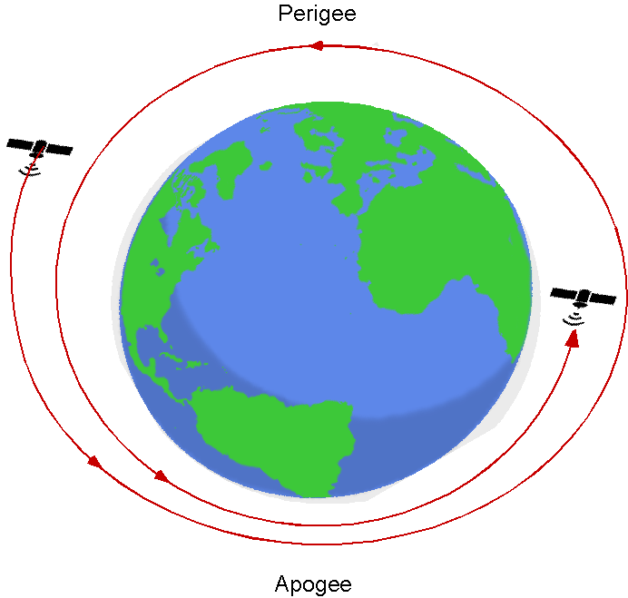
Analysis
It is difficult to predict orbital decay with the certainty that might be desired because of the variations in density in the upper atmosphere from tides, seasonal variations, solar activity, and other factors. However, reasonable estimates can still be made by using certain assumptions. The process involves an estimation of the aerodynamic drag force,  , on the satellite, which can be expressed conventionally as
(129) 
where is its orbital velocity. Without any other specific information, an ISA model for the extended atmosphere can represent the density,  . The reference area,
  , and the drag coefficient,
  , in Eq. 129 will depend on the exact shape of the satellite. It is often assumed that in the absence of specific information, then
  in the very outer regions of the atmosphere in the low-density or rarefied flow, increasing to
  when approaching an orbital altitude of 150 km. It is found that because of the eccentricity of most satellite orbits, the decay is more rapid at the apogee when it dips further into the atmosphere than the perigee, which, on average, tends to circularize the orbit.
For a satellite in an assumed circular orbit, the orbital velocity can be approximated as
(130) 
where is the Earth’s mass and is the average radius of the satellite’s orbit. The aerodynamic drag acts opposite to the satellite’s velocity, causing a loss of energy and a gradual reduction in the orbital radius.
The energy of the satellite in a circular orbit is
(131) 
where is the mass of the satellite. The time rate of change of energy from the creation of aerodynamic drag will be
(132) 
Substituting the forgoing expressions for and , i.e., Eqs. 129 and 130, respectively, gives
(133) 
Using Eq. 131, the time rate of change of energy is also given by
(134) 
Equating Eqs. 133 and 134 gives
(135) 
and rearranging gives
(136) 
the minus sign confirming an orbital decay. The orbital speed is given by Eq. 130, so that
(137) 
Therefore, substituting and rearranging gives
(138) 
where the grouping  is classically known as the ballistic coefficient[2] and is given the symbol
  . Notice that the units of are mass per unit area.
The significance of Eq. 138 shows that the rate of decay of the orbital radius, , is proportional to the aerodynamic drag coefficient, , the cross-sectional reference area, (on which the drag coefficient will be based), the atmospheric density, , and inversely proportional to the mass of the satellite, . The decay rate also depends on the speed of the satellite, , and its orbital radius, , with faster and closer satellites suffering more from orbital decay, as might be expected.
Notice also that the higher the value of the ballistics coefficient, , the lower the rate of orbital decay, an effect analogous to maximizing the range and velocity of a projectile. Because of their high values of , satellites also tend to have very high values of , typically between 100 for a small satellite[3] to over 5,000 for something like the ISS.
Dimensionless Form
The orbital decay can also be expressed in dimensionless form. If it is assumed that
(139) 
where  is some function to be determined, i.e., it depends on seven parameters, then a dimensional analysis will give that
(140) 
where  is some other function. The latter grouping in Eq. 140 is a buoyancy term, arising in hydrodynamics and aerodynamics, but of no consequence in space. Therefore, it can be concluded for the orbital decay problem that
(141) 
It will be seen that the dimensionless decay rate,  , is a function of the aerodynamic drag coefficient, , and a second dimensionless parameter that is the ratio of potential to kinetic energy, i.e.,
(142) 
This parameter indicates the ratio of gravitational energy to kinetic energy[4] for the satellite’s orbit. It also helps assess the relative dominance of gravitational forces compared to the centrifugal forces keeping the satellite in orbit, as summarized in the figure below.
If the value of  , then gravitational forces dominate, and the satellite remains in a stable orbit (assuming no other perturbations). If the value of
  , then orbital decay begins. The satellite will gradually lose altitude and eventually re-enter the atmosphere.
Consequences of Orbital Decay
Atmospheric drag significantly affects the LEO altitudes of crewed Earth-orbit spacecraft and satellites, even those at relatively high LEO, such as the Hubble Space Telescope, which has  540 km. Therefore, when the orbital decay reaches a critical level, a satellite must be boosted back into its initial orbit. Sufficient propellant must be carried onboard the satellite to ensure this can be done. The propellant required depends on the satellite’s mission requirements, projected life, and the rate of orbital decay. The ISS, for example, needs a regular altitude boost to counteract the effects of orbital decay. About once a month, the ISS fires its thrusters to recover its orbital altitude, a maneuver called a reboost. Accurately estimating the propellant required for a satellite in LEO is crucial, as having too little can cause a mission failure, while carrying too much propellant is just unnecessary weight and cost.
Typically, satellites in LEO exceeding a radial decay rate of approximately  km/s are considered to be in a critical state of orbital decay. For a satellite with
  7.5 km/s (similar to the ISS in LEO), a radial decay rate exceeding that threshold could see a significant orbital decay over a relatively short period. Typically, if a spacecraft comes within 160 km of the Earth’s surface, it will likely be in an irrecoverable orbit because of aerodynamic drag. It is unlikely that sufficient propellant is available to correct the orbit unless the intention is to de-orbit the satellite and take it out of commission. Therefore, the spacecraft will enter into a “graveyard spiral,” with its burn-up and disintegration typically starting at an altitude of about 80 km.
Atmospheric Re-entry
Sending astronauts into orbit or beyond is challenging enough, but getting them back safely to Earth brings up a whole new set of technical challenges. As shown in the figure below, this artist’s vision of a flaming spacecraft hurtling toward the Earth is close to the physical truth. The high re-entry velocities, which can reach Mach 12 and more, create tremendous amounts of friction on the spacecraft, creating heat. So much heat is produced during the re-entry that the spacecraft must be designed with a thermal protection system (TPS), such as a heat shield, so that it does not burn up and vaporize.
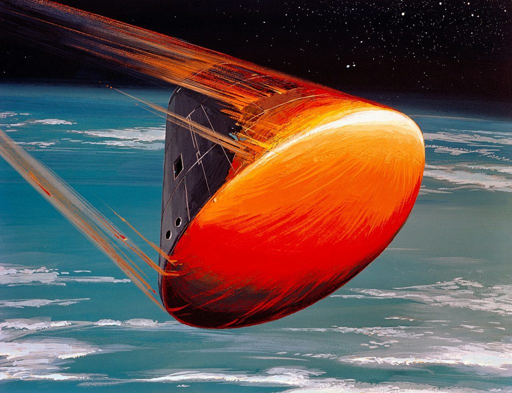
Work by the NACA showed that sharp objects flying at hypersonic speeds get too hot from kinetic heating and would melt. Therefore, the preference for a re-entry shape is a bluff or blunt body, which causes the primary shock waves to stand off from the spacecraft’s surface, as shown in the figure below, reducing the kinetic heating and creating high drag to slow it down. While the process still creates significant heat, blunt body shapes are always preferred, giving the required high value of the ballistic coefficient. Some shapes, such as the Space Shuttle and SpaceX’s Starship, can also create lift, allowing the descent speed and trajectory of re-entry to be controlled within certain bounds.
 During re-entry, the spacecraft experiences gravitational acceleration, pulling it toward Earth while simultaneously encountering aerodynamic drag opposing its motion, as described previously. The decelerations as the spacecraft enters the denser lower atmosphere may be significant, ranging up to 5 g. The balance between gravitation and aerodynamic forces governs the deceleration and descent profile of the spacecraft as it descends through varying atmospheric conditions. Understanding these forces is crucial for predicting and optimizing the trajectory to ensure a safe and controlled descent.
Most spacecraft designed to re-enter the Earth’s atmosphere for a landing will follow a ballistic or semi-ballistic trajectory, as shown in the figure below. The key to a safe landing is careful energy management and the complete depletion of the initial orbital energy. The re-entry flight path has a very steep angle, but is of relatively short duration. The steep re-entry angle creates atmospheric drag, slowing the spacecraft and progressively dissipating its potential and kinetic energy. In this regard, the spacecraft free-falls through the upper atmosphere at hypersonic Mach numbers, slowing down gradually as the atmosphere becomes denser. The lower atmosphere creates significant aerodynamic drag, which will cause the spacecraft to become subsonic. The final stages of a landing require the deployment of parachutes and perhaps a final retro-burn, so that the spacecraft lands softly into the sea or onto land.
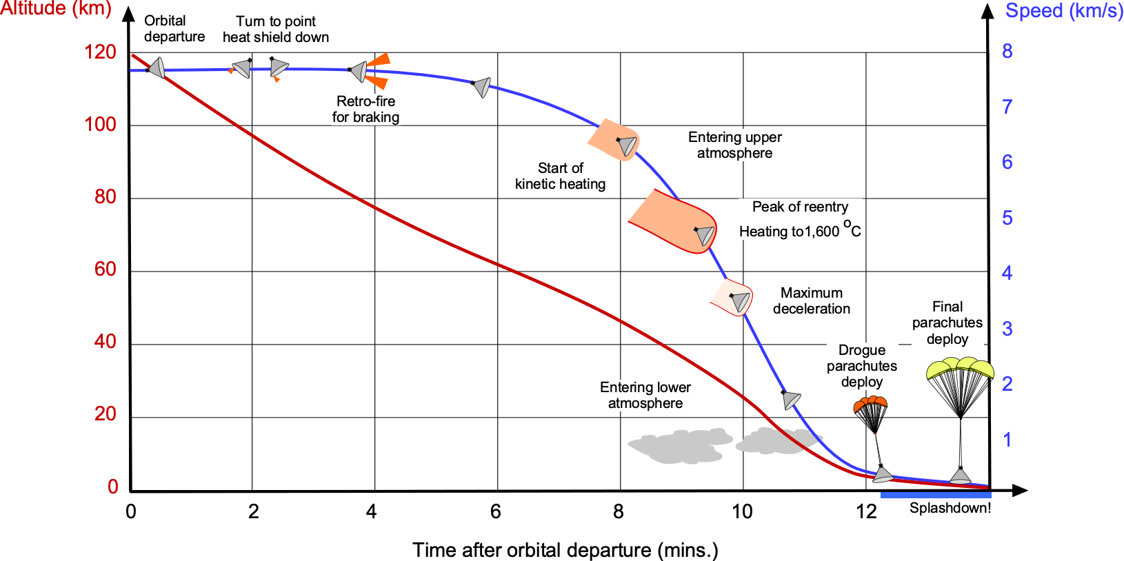
The re-entry trajectory analysis involves solving the differential equations of motion that incorporate gravity and aerodynamic drag forces. Given the complexity of the problem, numerical methods are employed. These methods can compute how the spacecraft’s velocity and altitude change in time as it descends through the atmosphere. The ISA model helps represent air density, temperature, and pressure change with altitude, which all influence the spacecraft’s dynamics and heat transfer characteristics during re-entry. Many simulations are typically performed with different assumptions, the final predicted trajectory being obtained with reasonable confidence.
Engineers can optimize re-entry trajectories to give specific landing locations, e.g., in the Gulf of Mexico or the Atlantic Ocean. This optimization often involves adjusting entry angles, velocities, and descent profiles to balance spacecraft capabilities while maintaining adequate safety margins. Managing kinetic heating is also important. The energy has to go somewhere, so a heat shield or other TPS provides thermal protection for the spacecraft. In some cases, the materials used for the TPS are designed to ablate and shed material to reduce the temperatures on the spacecraft. Advancements in computational fluid dynamics (CFD) and heat transfer simulations also allow for analyzing the spacecraft’s TPS, which is crucial for shielding the spacecraft from the intense heat generated during re-entry.
Summary & Closure
The ability to successfully engineer rockets and spacecraft has already made it possible for humankind to reach space. They have been used to study other planets and our own world. Planetary exploration using probes will continue in the decades to come, perhaps at an accelerated rate. Humans will likely return to the Moon before the end of this decade. However, the technical and other challenges in sending humans to even our nearest planets, including Mars, remain a much more ambitious technical goal. Nevertheless, humankind will likely continue to justify means to explore space, partly because commercial space endeavors have revitalized the public’s interest in space. In addition, new space technologies, including reusable launch vehicles and more efficient rocket engines, will continue to significantly reduce the costs of launching payloads into space.
Sending humans back to the Moon, Mars, and into deep space will be a highly ambitious goal that requires overcoming a range of technical and other challenges, including radiation exposure, life support, propulsion systems, habitat and resource utilization, human performance and health, cost and funding, technological advancements, and mission design and operations. Space exploration continues to push the boundaries of science and technology and helps us answer some of the biggest questions about our universe. The development of the International Space Station and partnerships between countries worldwide have enabled long-duration human spaceflights, leading to even more significant scientific discoveries and technological advancements that benefit space exploration and life on Earth.
5-Question Self-Assessment Quickquiz
For Further Thought or Discussion
- Can you hit a golf ball hard enough to send it into orbit around the Earth? What about if you were on the Moon? Could you hit a golf ball into a lunar orbit?
- Assume that someone dug a hole from one point on the surface of the Earth all the way to its core and then out the other side. What would happen if you then jumped in the hole? Would you pop out on the other side of the Earth?
- Is there any gravity at the center of the Earth? Hint: Consider the effects of gravity on one mass located inside a larger mass.
- Prove that the potential at a point outside a spherical shell of mass is
 , where is the distance to the point from the center of the shell.
 - As a spacecraft leaves the Earth and heads to the Moon, it will progressively overcome the Earth’s gravity and be gradually attracted by the Moon’s gravity. At what point between the Earth and the Moon will the gravitational effects be in perfect balance?
- As a pressure or sound source moves in the air, a Doppler effect comes into play relative to a fixed observer. What might happen to a light source as it nears the speed of light?
Other Useful Online Resources
Visit the following websites to learn more about space and orbital mechanics:
- A lecture by Dr. Steven Hawking: “Why we should go into space.”
- Carl Sagan’s 1994 “Lost” Lecture: “The Age of Exploration.”
- Carl Sagan Lecture: Cosmos – Galaxies
- The entire series of Carl Sagan video lectures.
- A rare interview with Neil Armstrong, the first person to walk on the Moon.
- A NASA video on: “Space Flight: The Application of Orbital Mechanics.”
- NASA talk: “Escaping Earth’s Gravity: Space Launch System.”
- NASA talk: “Path to Mars and Asteroid Mission: The First Step.”
- NASA video: ” Space Flight: The Application of Orbital Mechanics.”
- 25 Mind-Blowing Facts About the Apollo Space Missions – Smithsonian Channel.
- Deriving Einstein’s most famous equation: Why does energy = mass x speed of light squared?
- The author is indebted to his teacher, Professor Archie Roy, who inspired many generations of engineering students about astronomy, space, and the future possibilities of space flight.
 ↵
↵ - In the conventional ballistics of projectiles, the ballistic coefficient, , of a bullet is a measure of its ability to overcome air resistance in flight. A higher value of means it will be faster when it reaches the target. ↵
- As a reference, a rifle bullet will have a value of
 0.1. ↵
 - It will be recognized that the classic Froude number used in hydrodynamics is simply the square root of this parameter, although, in the present context, which relates to orbital mechanics, the parameter is most meaningful when left as it is, which is as a ratio of energy states. ↵
