Worked Examples: Fluid Flows & Fluid Dynamics

J. Gordon Leishman

doi:https://doi.org/10.15394/eaglepub.2022.1066.9

70 Worked Examples: Fluid Flows & Fluid Dynamics

These worked examples have been fielded as homework problems or exam questions.

Worked Example #1

Examine the flow visualization of the circular cylinder in the photograph below. Discuss the nature of the flow in Zone A. Is the flow here steady or unsteady? Identify the streamlines. Explain the nature of their curvature and spacing. Where is the highest velocity, and where is the lowest? Discuss the nature of the flow in Zone B. Is the flow here steady or unsteady? Where does the flow separate from the cylinder? What happens to the flow after that? Discuss the nature of the flow in Zone C. Is the flow here steady or unsteady? Is it laminar or turbulent, and where? Is it transitional? Identify any eddies or vortices. Discuss the nature of the flow in Zone D. While turbulent and unsteady, are there still any laminar flow regions? Why does the original smoke diffuse?

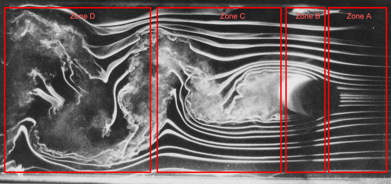
Zone A: The flow is steady and primarily laminar in Zone A. The streamlines are smooth, indicating that the flow is turbulence-free. The streamlines are straight and closely spaced near the front of the cylinder. The streamline curvature is relatively mild as they wrap around the leading edge half of the cylinder. The highest velocity occurs where the streamlines are closest together, which occurs near the equator of the cylinder. There is a stagnation flow region on the front of the cylinder, where the flow is brought to rest. The curvature of the streamlines increases as they approach the cylinder, and the spacing between them decreases, which implies that the flow is accelerating as it passes around the cylinder.

Zone B: The flow in Zone B is transitioning to a more unsteady state. This is the region where flow separation occurs from the cylinder. The flow begins to separate from the surface of the cylinder near its equator; you can identify the separation point where the streamlines start to diverge from the surface. After the point of separation, the flow begins to form turbulent eddies, and there is evidence of recirculation where the flow curls back on itself. This marks the onset of the unsteady wake behind the cylinder, and disturbances in the flow start to appear as it loses all of its initial laminar characteristics.

Zone C: The flow in Zone C is unsteady and turbulent. This region is characterized by the formation of larger eddies and vortices, which are visible in the image as swirling, rotational flow patterns. The flow is likely still in some transitional state between laminar and fully turbulent. The eddies grow more prominent as the flow develops downstream, and the flow becomes increasingly turbulent. Several discrete eddies and vortices can be observed in this region. These are the characteristic features of the unsteady wake behind the cylinder, often called a Kármán vortex street.

Zone D: The flow in Zone D is turbulent and would be classified as unsteady. By default, turbulent flows are unsteady flows. The vortices become more random and spread out when moving further downstream. Although the flow is predominantly turbulent, there may still be small laminar pockets or other remnants of laminar flow at specific points in the flow field, mainly where the turbulence is not yet fully developed. The original smoke filaments introduced into the flow diffuse because of the turbulent mixing in this zone. As the flow transitions to a fully turbulent state, the smoke filaments lose their coherence, and the smoke rapidly spreads out because of increased diffusion caused by turbulent mixing.

Worked Example #2

Two pipes with diameters ${d_1}$ and ${d_2}$ converge to form a single pipe with diameter ${d}$ . If a liquid flows with a velocity of ${V_1}$ and ${V_2}$ in the two pipes, respectively, what will be the flow velocity ${V_3}$ in the third pipe? Hint: Assume steady, one-dimensional, incompressible flow with no losses.

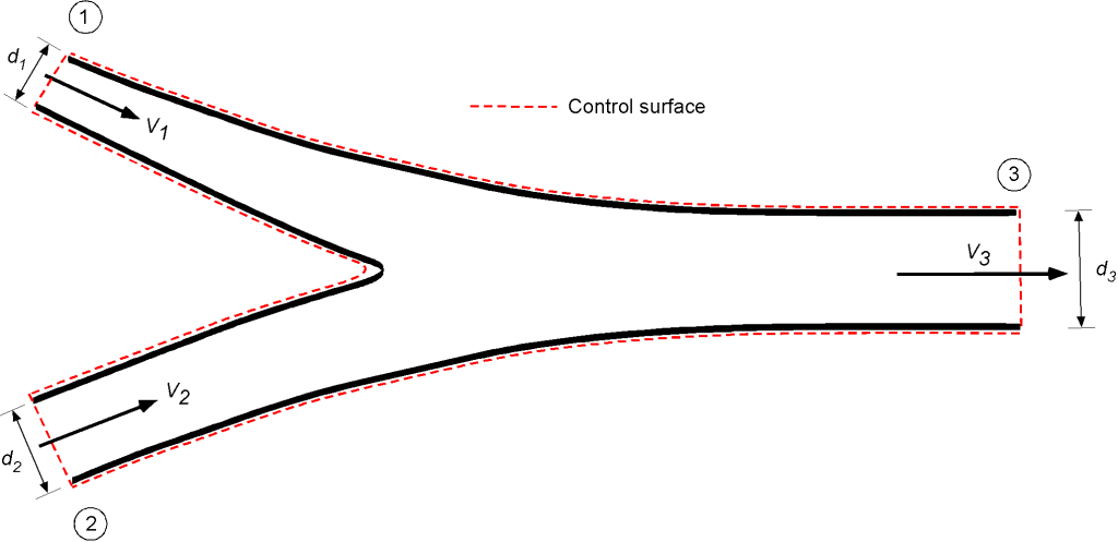
In this case, two pipes merge to produce one pipe. Conserving mass and using average flow properties, then

$\overbigdot{m} = \mbox{constant} = \varrho_1 V_1 A_1 + \varrho_2 V_2 A_2 = \varrho_3 V_3 A_3$

If the fluid is a liquid then the assumption that $\varrho$ = $\varrho_1$ = $\varrho_2$ = $\varrho_3$ = constant is justified so

$Q = \mbox{constant} = V_1 A_1 + V_2 A_2 = V_3 A_3$

Therefore, the flow velocity in the third pipe is

$V_3 = \frac{V_1 A_1 + V_2 A_2}{A_3} = \frac{V_1 (\pi \, d_1^2/4) + V_2 (\pi \, d_2^2/4)}{ (\pi \, d^2/4)} = \frac{V_1 \, d_1^2 + V_2 \, d_2^2}{d^2}$

Worked Example #3

Air flows steadily through a horizontal pipe of a constant circular cross-sectional area. The air temperature is steady at $T_{\rm air} = 26^{\circ}$ C along the flow direction. At point A, the static pressure is $p_A = 3 \times 10^5$ Pa, and the mean velocity is $V_A = 110$ m/s. At point B, the static pressure is $p_B = 2 \times 10^5$ Pa. What is the average flow velocity at B? Use $R$ = 287.057 J kg $^{-1}$ K $^{-1}$ and assume no losses.

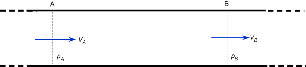
The requirement for flow velocities suggests the use of the continuity equation, which can be written as

$\varrho_A V_A A_A = \varrho_B V_B A_B$

Notice that the density of the air is not given, but the pressures and the temperature $T_{\rm air} = T_A = T_B$ are, so using the equation of state gives

$\varrho_A = \frac{p_A}{R \, T_A} = \frac{3 \times 10^5}{287.057 \times (26.0 + 273.15)} = 3.494~\mbox{kg/m${^3}$}$

Likewise

$\varrho_B = \frac{p_B}{R \, T_B} = \frac{2 \times 10^5}{287.057 \times (26.0 + 273.15)} = 2.329~\mbox{kg/m${^3}$}$

The use of the continuity equation gives

$V_B = \left( \frac{\varrho_A}{\varrho_B} \right) \left( \frac{A_A}{A_B} \right) V_A = \left( \frac{3.494}{2.329} \right) 110.0 = 165.04~\mbox{m/s}$

noting that

$\left( \frac{A_A}{A_B} \right) = 1$

Worked Example #4

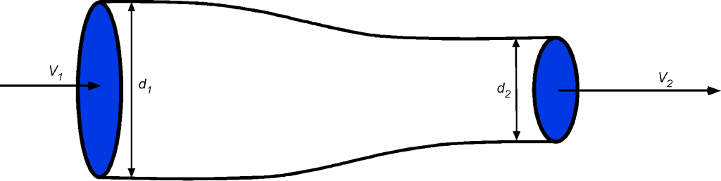
A gas of density 1.7 kg/m ${^3}$ flows through a pipe with a volume flow rate of 0.12 m ${^3}$ /s. The pipe has an inlet section diameter of ${d_1}$ of 21 cm and an outlet section diameter ${d_2}$ of 9 cm. Assuming an ideal incompressible fluid flow, calculate the flow velocities at the pipe’s inlet and outlet, i.e., ${V_1}$ and ${V_2}$ , respectively.

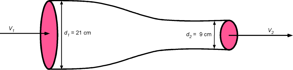
From the information given, assuming a one-dimensional, steady, incompressible, inviscid flow is reasonable. The flow rates, velocities, and Mach numbers are low enough that compressibility effects can be neglected. Let the inlet be condition 1 and the outlet condition 2. The continuity equation can be used to relate the inlet and outlet conditions, i.e.,

$\overbigdot{m} = \varrho A_1 V_1 = \varrho A_2 V_2 = \mbox{constant}$

Or because the flow is assumed incompressible, then just

$Q = A_1 V_1 = A_2 V_2 = \mbox{constant} = 0.12~\mbox{m${^3}$/s}$

We see that

$V_1 = \frac{Q }{A_1}$

and

$V_2 = \frac{Q }{A_2}$

We can calculate $A_1$ , i.e.,

$A_1 = \frac{\pi d_1^2}{4} = \frac{\pi \, 0.21^2}{4} = 0.0346~\mbox{m${^{2}}$}$

and also $A_2$ , i.e.,

$A_2 = \frac{\pi d_2^2}{4} = \frac{\pi \, 0.09^2}{4} = 0.00636~\mbox{m${^{2}}$}$

so that

$V_1 = \frac{Q }{A_1} = \frac{0.12}{0.0346} = 3.47~\mbox{m/s}$

and

$V_2 = \frac{Q }{A_2} = \frac{0.12}{0.00636} = 18.87~\mbox{m/s}$

We have confirmed that the flow velocities are very low, much lower than a Mach number of 0.3, so the initial assumption of incompressible flow was justified.

Worked Example #5

A flowing liquid enters a pipe of diameter ${d_1}$ with a velocity ${V_1}$ . What will the velocity ${V_2}$ of the liquid be at the exit if the diameter of the pipe progressively reduces to $d_2 = 0.6d$ ? Hint: Assume a one-dimensional ideal flow.

Conserving mass and using the continuity equation with average flow properties (i.e., one-dimensional flow) gives

$\oiint_S \vec{V} \bigcdot d\vec{S} = \overbigdot{m} = \mbox{constant} = \varrho_1 V_1 A_1 = \varrho_2 V_2 A_2$

Because the fluid is a liquid, the assumption that $\varrho$ = constant is justified. So, the continuity equation is reduced to

$Q = \mbox{constant}$

In this case

$Q = V_1 \left( \frac{\pi d^2}{4} \right) = V_2 \left(\pi \frac{(0.6d)^2}{4} \right) = V_2 \left(\frac{0.36 \pi d^2}{4} \right) = 0.36 V_2 \left(\frac{\pi d^2}{4} \right)$

where ${V_2}$ is the exit velocity. Rearranging gives

$V_2 = \frac{V_1}{0.36} = 2.78 V_1$

Worked Example #6

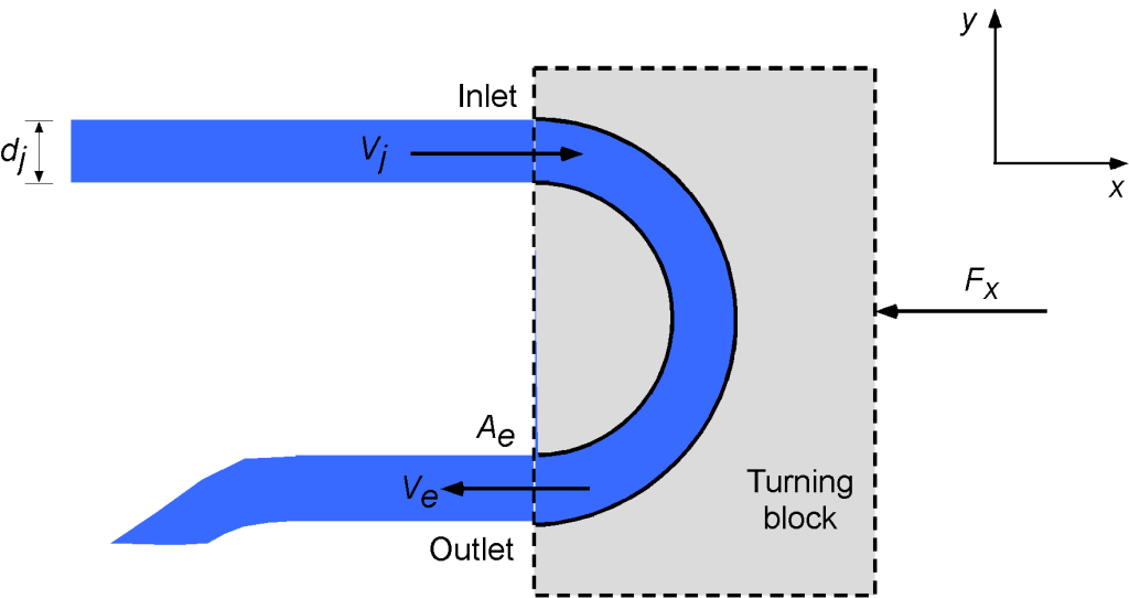
Consider the flow-turning block shown below. A circular jet of water with diameter $D_j =$ 10 cm at a velocity $V_j = 13$ ms $^{-1}$ enters the block. The block turns the water back through 180 degrees and then exits through an orifice with an area $A_e$ of 120 cm ${^{2}}$ . First, find the velocity $V_e$ of the water exiting the block. Second, determine the force $F_x$ required to hold the block in place. Hint: Assume one-dimensional flow.

First, the conservation of mass is applied to the inlet and outlet flow from the control volume, i.e., for a steady flow.

$\oiint_S \varrho \, \vec{V} \bigcdot d\vec{S} = 0$

and in one-dimensional form, then

$-\varrho V_j A_j + \varrho V_e A_e = 0$

or

$\varrho V_j A_j = \varrho V_e A_e = \overbigdot{m}$

The fluid is water so $\varrho =$ constant and so

$V_j A_j = V_e A_e$

Rearranging to solve for the exit velocity $V_e$ gives

$V_e = V_j \left( \frac{A_j }{A_e} \right) = \left( \frac{ \displaystyle{\frac{\pi}{4} } D_j^2}{A_e} \right) V_j$

Substituting the known values gives

$V_e = \left( \frac{ \displaystyle{\frac{\pi}{4} } D_j^2}{A_e} \right) V_j = \left( \frac{ \displaystyle{\frac{\pi}{4} } 0.1^2}{0.012} \right) 13.0 = 8.51\mbox{m s$^{-1}$}$

Second, from the principle of conservation of momentum, then

$\vec{F} = \oiint_S (\varrho \, \vec{V} \bigcdot d\vec{S}) \vec{V}$

where $\vec{F}$ on the fluid from the block. In this case, then

$\vec{F} = \overbigdot{m} (-V_j ) - \overbigdot{m} V_e = -\overbigdot{m} \left( V_e + V_j \right)$

The minus sign reminds us that the force on the fluid is to the left, i.e., in the negative ${x}$ direction. The mass flow rate is conserved, so

$\overbigdot{m} = \varrho V_j A_j =\varrho V_e A_e = 1,000.0 \times 8.51 \times 0.012 = 102.12~\mbox{kg/s}$

where the density of water has been assumed to be 1,000 kg/m ${^3}$ , and so

$\vec{F} = \overbigdot{m} \left( V_e + V_j \right) = 102.12 \left( 8.51 + 13.0\right) = 2,196.6~\mbox{N}$

Therefore, the reaction force on the block is to the right, i.e., in the positive ${x}$ direction. Therefore, the force to restrain the block will be 2196.6 N toward the left.

Worked Example #7

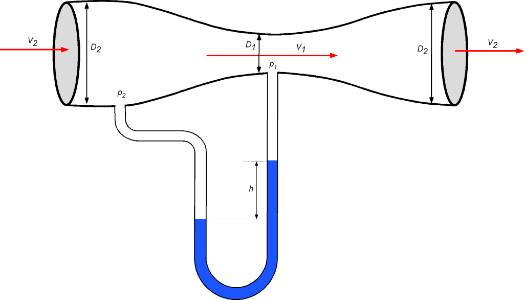
An incompressible gas flow in a pipe is passed through a venturimeter. The pipe diameter is $D_2$ = 4.1 inches, and the diameter of the throat of the venturimeter $D_1$ = 2.2 inches. The gas flow in the main pipe has a velocity ${V_2}$ = 14.3 ft/s. If the static pressure difference between the venturi’s inlet and throat is measured using a U-tube water manometer, then calculate the height ${h}$ between the two columns. Assume 1-dimensional flow and no losses. Also assume that $\varrho_{w}$ = 1.94 slug/ft ${^3}$ and $\varrho_{\rm gas}$ = 0.0023 slug/ft ${^3}$ .

Assuming steady, 1-dimensional flow, applying the continuity equation between the inlet and the throat gives

$\varrho_1 \, A_1\, V_1 = \varrho_2 \, A_2 \, V_2$

And because $\varrho_1 = \varrho_2 = \varrho =$ constant in this case (the flow is stated to be incompressible), then

$A_1 \, V_1 = A_2 \, V_2$

Therefore, solving for ${V_1}$ gives

$V_1 = \frac{A_2 \, V_2}{A_1} = \frac{\left(\displaystyle{\frac{\pi}{4}}\right)D_2^2 \, V_2}{\left(\displaystyle{\frac{\pi}{4}}\right)D_1^2} = \frac{\left(\displaystyle{\frac{4.1}{12}}\right)^2 \times 14.3 }{\left(\displaystyle{\frac{2.2}{12}} \right)^2} = \frac{4.1^2 \times 14.3 }{2.2^2} = 49.67 \mbox{ ft/s}$

The application of Bernoulli’s equation gives

${ p_1 + \frac{1}{2} \, \varrho_{\rm gas}\, V_1^2 + \varrho_{\rm gas} \, g \, z_1 = p_2 + \frac{1}{2} \, \varrho_{\rm gas} \, V_2^2 + \varrho_{\rm gas} \, g \, z_2 }$

There is no change in the vertical height of the mean flow in this case, so $z_1 = z_2 = 0$ and

$p_1 + \frac{1}{2} \, \varrho_{\rm gas}\, V_1^2 = p_2 + \frac{1}{2} \, \varrho_{\rm gas} \, V_2^2$

Rearranging for the pressure difference $p_2 - p_1$ gives

$p_2 - p_1 = \frac{1}{2}\varrho_{\rm gas}\left(V_1^2 - V_2^2\right)$

The U-tube manometer will measure this static pressure difference $p_2 - p_1$ , so using the hydrostatic equation, the pressure difference is

$p_2 - p_1 = \varrho_{w} \, g \, h$

making sure the density of water is used. Therefore, equating the latter two equations gives

$\varrho_{w} \, g \, h = \frac{1}{2}\varrho_{\rm gas}\left(V_1^2 - V_2^2\right)$

and solving for ${h}$ leads to

$h = \frac{\varrho_{\rm gas}}{2 \, \varrho_{w} \, g}\left(V_1^2 - V_2^2\right) = \frac{0.0023}{2 \times 1.94 \times 32.17}\left( 49.67^2 - 14.3^2\right) = 0.0417~\mbox{ft}$

Worked Example #8

For gases undergoing adiabatic compression or expansion, the bulk modulus is related to the pressure using $K_b = \gamma \, p$ . If changes in density in an incompressible flow must be less than 5\%, then show that to ensure incompressible behavior, the flow Mach number, $M = V/a$ , must be less than 0.3. Hint: You may assume that $\Delta p \approx -\dfrac{1}{2} \varrho \Delta V$ and $a = \sqrt{\gamma \ R \ T}$ and $p = \varrho R \, T$ .

For gases undergoing adiabatic compression or expansion, the bulk modulus is given by

$K_b = \gamma \, p$

where $\gamma$ is the ratio of specific heats. Using the result that

$\frac{\Delta \varrho}{\varrho} = -\frac{\Delta p}{K_b}$

then substituting $K_b = \gamma \, p$ gives

$\frac{\Delta \varrho}{\varrho} = -\frac{\Delta p}{\gamma \, p}$

Assuming $\Delta p \approx -\dfrac{1}{2} \varrho \, V^2$ as given in the question, then

$\frac{\Delta \varrho}{\varrho} = -\frac{\dfrac{1}{2} \varrho \, V^2}{\gamma \, p}$

Using $p = \varrho \, R \, T$ into $\gamma \, p$ gives

$\gamma \, p = \gamma \, \varrho \, R \, T$

The speed of sound $a$ is given by $a = \sqrt{\gamma \, R \, T}$ , so $\gamma \, R \, T = a^2$ . Substituting $\gamma \, R \, T = a^2$ gives

$-\frac{\Delta \varrho}{\varrho} = \frac{\dfrac{1}{2} V^2}{a^2} = \dfrac{1}{2} M^2$

For incompressible behavior, changes in density must be less than 5\%, i.e.,

$\frac{\Delta \varrho}{\varrho} = \dfrac{1}{2} M^2 < 0.05$

so that

$\frac{1}{2} M^2 < 0.05$

Solving for $M$ gives $M < 0.316$ . Therefore, to ensure incompressible behavior in practical applications, the flow Mach number must be less than about 0.3.

Worked Example #9

If $u = 2x$ and $v = -2y$ , is this a physically possible flow?

The flow will be physically possible if it satisfies continuity, i.e., the divergence of the velocity field is zero. For a two-dimensional flow in the ${x}$ – ${y}$ plane, then

$\frac{\partial u}{\partial x} + \frac{\partial v}{\partial y} = 0$

In this case, $u = 2x$ and $v = -2y$ , so

$\frac{\partial u}{\partial x} + \frac{\partial v}{\partial y} = \frac{\partial (2x)}{\partial x} + \frac{\partial (-2y)}{\partial y} = 2 - 2 = 0$

So, we have proved that this specific flow field is indeed physically possible.

Worked Example #10

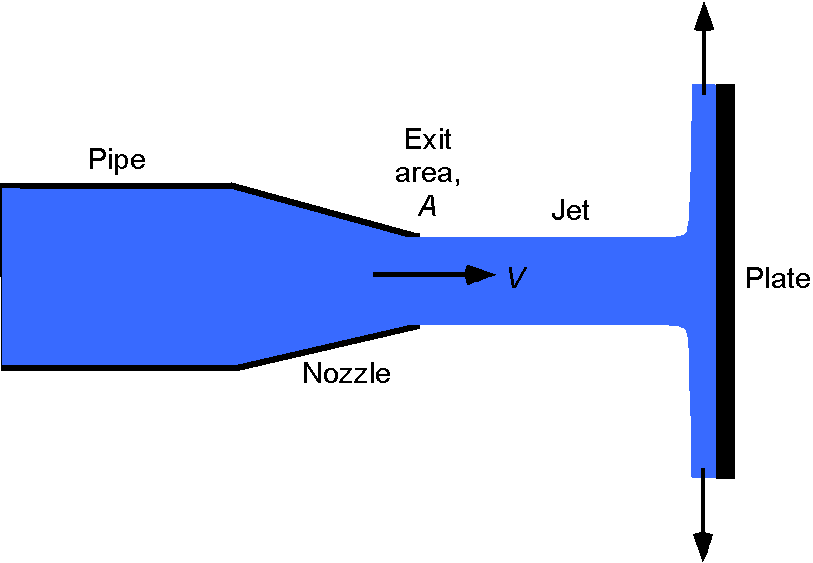
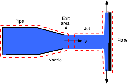
A water jet with velocity $V$ that exits from a nozzle strikes a vertical plate. The exit area of the nozzle is $A$ . Find an expression for the horizontal force on the plate. If the volume flow rate through the nozzle is 0.5 m ${^{3}}$ s $^{-1}$ and the diameter of the jet is 5 cm, then find the force on the plate in Newtons. The density of water can be assumed to be 1,000 kg m ${^{-3}}$ .

The force on the plate is related to the force of the fluid and the nozzle’s exit velocity. Using the momentum equation and assuming that the flow is steady and inviscid, then the force on the plate from the water jet is equal to the time rate of change in horizontal momentum, i.e.,

$-F = \oiint_S (\varrho \, \vec{V} \bigcdot d\vec{S}) \vec{V}$

Using a one-dimensional assumption, then

$F = \overbigdot{m} V - 0$

The use of the continuity equation gives

$\varrho V A = \overbigdot{m}$

and because we are dealing with water, then it is incompressible, so

$V A = Q = 0.5~\mbox{m${^{3}}$ s$^{-1}$}$

The value of $V$ is

$V = \frac{Q}{A} = \frac{0.5}{\pi d^2/4} = \frac{0.5}{\pi (0.05)^2/4} = 254.65~\mbox{m s$^{-1}$}$

Therefore, the force on the plate is

$F = \overbigdot{m} V = \left( \varrho Q \right) V = 1,000 \times 0.5 \times 254.65 =127.33~\mbox{kN}$

Worked Example #11

Water flows into a container through pipes 1 and 3 and simultaneously exits through pipe 2. The flow rates are adjusted such that the height ${h}$ of water in the container stays constant. The volume flow rate $Q_3 = 0.015$ m ${^3}$ /s and also $V_{1} = 3.4$ m/s, $D_1 = 0.05$ m and $D_2 = 0.075$ m. From this information, determine the value of ${V_2}$ . Make any assumptions that may be justified.

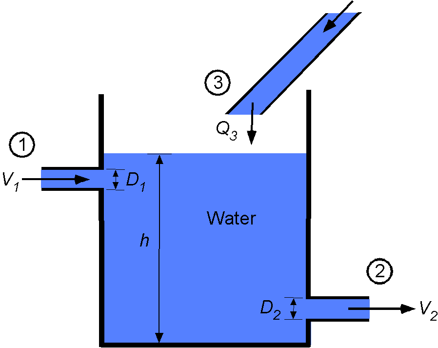
If the level ${h}$ stays constant, then the system’s net mass (or volume) flow is constant in that the mass of water coming in per unit time is equal to the mass (or volume) of water leaving per unit time. In terms of the problem parameters, then

$Q = Q_1 + Q_3 = Q_2$

where $Q_3 = 0.015$ m ${^3}$ /s. Remember that

$Q = A V$

so

$V = \frac{Q}{A}$

and so

$A_1 V_{1} + Q_3 = A_2 V_2$

And solving for ${V_2}$ , which is what we are asked to find, then

$V_2 = \frac{A_1 V_{1} + Q_3}{A_2}$

We are given the diameters $D_1 = 0.05$ m and $D_2 = 0.075$ m so

$A_1 = \frac{\pi D_1^2}{4} = \frac{\pi \times 0.05^2}{4} = 0.00196~\mbox{m${^{2}}$}$

and

$A_2 = \frac{\pi D_2^2}{4} = \frac{\pi \times 0.075^2}{4} = 0.00442~\mbox{m${^{2}}$}$

so

$V_2 = \frac{A_1 V_{1} + Q_3}{A_2} = \frac{ 0.00196 \times 3.4 + 0.015}{0.00442} = 4.901~\mbox{m/s}$

Worked Example #12

A rigid tank of volume ${\cal{V}}$ has air pumped into it at a constant mass flow rate. Find the density and pressure in the tank as a function of time if the initial density and pressure are $\varrho_0$ and $p_0$ , respectively. You may assume that the process is isothermal. Make any other assumptions that can be justified.

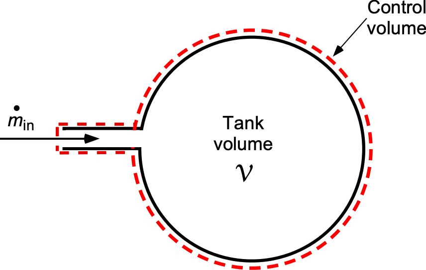
This is an unsteady flow problem because a mass of gas is pumped into a fixed volume, and for mass conservation, the gas density must increase in time. The general form of the continuity equation is

$\frac{\partial}{\partial t}\oiiint \varrho \ d {\cal{V}} + \oiint_S \varrho \, \vec{V} \bigcdot d\vec{S} = 0$

In this case

$\oiint_S \varrho \, \vec{V} \bigcdot d\vec{S} = -\overbigdot{m}_{\rm in}$

also

$\frac{\partial}{\partial t}\oiiint \varrho \, d{\cal{V}} = {\cal{V}}\frac{d \varrho}{dt}$

We will assume uniform mixing, and so the density inside the volume is uniform, so we have

${\cal{V}} \frac{d \varrho}{dt} = \overbigdot{m}_{\rm in}$

Integrating using the separation of variables gives

$\int_{\varrho_0}^{\varrho} d \varrho = \frac{ \overbigdot{m}_{\rm in}}{{\cal{V}}} \int_{t_0}^{t} dt$

so

$\varrho = \varrho_0 + \frac{ \overbigdot{m}_{\rm in}}{{\cal{V}}} \left( t - t_0 \right)$

which shows that the density of the gas increases linearly with time. The corresponding pressure can be obtained from the equation of state, i.e., $p = \varrho R T$ . If the process is isothermal, then $T = T_0$ , and so

$p = \varrho_0 \, R \, T_0 + \frac{ R \, T_0 \, \overbigdot{m}_{\rm in}}{{\cal{V}}} \left( t - t_0 \right) = p_0 + \frac{R \, T_0 \, \overbigdot{m}_{\rm in}}{{\cal{V}}} \left( t - t_0 \right)$

Worked Example #13

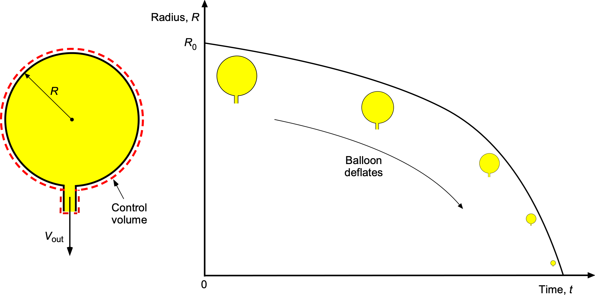
A spherical balloon of initial radius $R = R_0$ is filled with a gas of density $\varrho$ . The gas is at low pressure and can be assumed to be incompressible. The balloon starts deflating at time $t = 0$ through a small circular opening of diameter ${d}$ . The velocity of the flow through the opening, $V_{\rm out}$ , can be assumed constant and one-dimensional. Assume the balloon is tethered so it does not fly away! Why would it do that anyway?

Formulate the problem using the integral form of the continuity equation.
Determine the rate at which the balloon’s radius changes with time.

For an incompressible gas, the continuity equation in integral form is

$\oiint_S \varrho \, \vec{V} \bigcdot d\vec{S} = -\frac{\partial}{\partial t} \iiint_{\cal{V}} \varrho d{\cal{V}}$

The volume of the balloon at any time $t$ is

${ {\cal{V}} (t) = \frac{4}{3} \pi \, R(t)^3 }$

Taking the time derivative

$\frac{\partial {\cal{V} }}{\partial t} = 4 \pi \, R(t)^2 \, \frac{dR}{dt}$

The outflow mass flow rate through the opening of diameter ${d}$ is

$\oiint_S \varrho \, \vec{V} \bigcdot d\vec{S} = \varrho V_{\rm out} \left( \frac{\pi d^2}{4} \right)$

where $V_{\rm out}$ is the flow velocity through the opening.

Using the continuity equation gives

$\varrho V_{\rm out} \left( \frac{\pi \, d^2}{4} \right) = -\frac{\partial}{\partial t} \left( \varrho \frac{4}{3} \pi \, R(t)^3 \right)$

The flow is incompressible, so

$V_{\rm out} \left( \frac{\pi \, d^2}{4} \right) = -\frac{\partial}{\partial t} \left( \frac{4}{3} \pi \, R(t)^3 \right) = -4 \pi \, R(t)^2 \frac{dR}{dt}$

Rearranging gives

${ V_{\rm out} = -\frac{16 \, R(t)^2}{d^2} \frac{dR}{dt} }$

and so

$\frac{dR}{dt} = -\frac{V_{\rm out} \, d^2}{16 R(t)^2}$

Separating variables and integrating gives

$\int R^2 \, dR = -\frac{V_{\rm out} \, d^2}{16} \int \, dt$

The solution is

$\frac{R^3}{3} = -\frac{V_{\rm out} \, d^2}{16} t + C$

The boundary condition is give as $t = 0$ , $R = R_0$ , so

$C = \frac{R_0^3}{3}$

Rearranging and simplifying gives

$R^3 = R_0^3 - \frac{3V_{\rm out} \, d^2}{16} t$

Therefore, the solution for the radius of the balloon as a function of time is

$R(t) = \left( R_0^3 - \frac{3V_{\rm out} \, d^2}{16} t \right)^{\frac{1}{3}}$

Worked Example #14

Identify and explain each term starting from the most general form of the continuity equation. Then, show and explain carefully how both of these general equations can be simplified for application to problems that involve: (a) steady, compressible flows, (b) incompressible flows, and (c) inviscid, one-dimensional, steady flows.

The general form of the continuity equation is

$\frac{\partial}{\partial t}\oiiint_{\cal{V}} \varrho \, d {\cal{V}} + \oiint_S \varrho \, \vec{V} \bigcdot d\vec{S} = 0$

The first term is the time rate of change of fluid mass inside the control volume, and the second is the net mass flow rate of fluid out of the control volume. Conservation of mass requires that the net sum be zero.

(a) Steady, compressible flow. In this case ${\partial/\partial t \equiv 0}$ so that

$\oiint_S \varrho \, \vec{V} \bigcdot d\vec{S} = 0$

which is a statement that an equal mass of fluid coming into a control volume per unit time will also leave the control volume simultaneously.

(b) Steady, incompressible flow. In this case, $\varrho$ = constant so that we can write

$\oiint_S \vec{V} \bigcdot d\vec{S} = 0$

This is a statement that the volume flow rate is conserved, i.e., an equal volume of fluid coming into a control volume per unit time will leave the control volume simultaneously.

(c) One-dimensional, steady flow. In this case, we must again retain the density in the integral, but if the flow is one-dimensional, then the flow properties can change only in one dimension, so for a fixed control volume with an inlet and outlet plane defined accordingly, by conserving mass we would end up with

$\oiint_S \vec{V} \bigcdot d\vec{S} = -\varrho_1 V_1 A_1 + \varrho_2 V_2 A_2 = 0$

or

$\varrho_1 V_1 A_1 = \varrho_2 V_2 A_2 = \overbigdot{m} = \mbox{constant}$

This is a common form of the continuity equation and is very useful for problem-solving when average flow properties are desired.

Worked Example #15

Starting from the most general form of the momentum equation, identify the meaning of each of the terms and show how the equation can then be simplified for application to problems involving: (a) Steady flows, (b) Steady, incompressible flows, (c) Steady, inviscid flow. (d) Unsteady flows with no body forces. In each case, explain the physical meaning of the terms in the respective equations.

The most general form of the momentum equation in integral form is

$\oiiint_{\cal{V}} \varrho \vec{f} _b d{\cal{V}} -\oiint_S p dS + \vec{F}_{\mu} = \frac{\partial}{\partial t}\oiiint_{\cal{V}} \varrho \, \vec{V} d {\cal{V}} + \oiint_S (\varrho \, \vec{V} \bigcdot d\vec{S}) \vec{V}$

In words: Body Forces + Pressure Forces + Viscous Forces = Time rate of change of momentum inside ${\cal {V}}$ from unsteadiness + Net flow of momentum out of ${\cal {V}}$ per unit time. It is a vector equation, so three scalar equations are rolled into one. This equation is very general and will apply to any flow.

(a) For steady flows, then ${\partial/\partial t \equiv 0}$ , and the reduced form of the momentum equation will be

$\oiiint_{\cal{V}} \varrho \vec{f}_b d{\cal{V}} - \oiint_S p dS + \vec{F}_{\mu} = \oiint_S (\varrho \, \vec{V} \bigcdot d\vec{S}) \vec{V}$

(b) For steady, incompressible flows then ${\partial/\partial t \equiv 0}$ and $\varrho =$ constant so

$\varrho \oiiint_{\cal{V}} \vec{f}_b d{\cal{V}} - \oiint_S p dS + \vec{F}_{\mu} = \varrho \oiint_S (\vec{V} \bigcdot d\vec{S}) \vec{V}$

(c) For steady, inviscid flow then ${\partial/\partial t \equiv 0}$ and $\vec{F}_{\mu} = 0$ so

$\oiiint_{\cal{V}} \varrho \vec{f}_b d{\cal{V}} - \oiint_S p dS = \oiint_S \varrho (\vec{V} \bigcdot d\vec{S}) \vec{V}$

(d) For unsteady flows with no body forces, then $\vec{f} _b$ = 0, so

$-\oiint_S p dS + \vec{F}_{\mu} = \frac{\partial}{\partial t}\oiiint_{\cal{V}} \varrho \, \vec{V} d {\cal{V}} + \oiint_S (\varrho \, \vec{V} \bigcdot d\vec{S}) \vec{V}$

Worked Example #16

Starting from the most general form of the energy equation, identify the meaning of each of the terms and show how the equation can be simplified for application to problems involving: (a) Steady flows, (b) Steady, inviscid flow, (c) Steady flows with no body forces, heat, or work addition. In each case, explain the physical meaning of the terms in the respective equations.

The most general form of the energy equation is

$\begin{eqnarray*} \oiiint_{\cal{V}} \overbigdot{q} \varrho \, d {\cal{V}} + Q_{\mu} -\oiint_{S} (p d\vec{S}) \bigcdot \vec{V} + \oiiint_{\cal{V}} ( \varrho \vec{f}_b d{\cal{V}}) \bigcdot \vec{V} + \overbigdot{W}_{\mu} + \overbigdot{W}_{\rm mech} = && \nonumber \\ \frac{\partial}{\partial t} \oiiint_{\cal{V}} \varrho \left( e + \frac{V^2}{2} + g z\right) d{\cal{V}} + \oiint_{S} (\varrho \, \vec{V} \bigcdot d\vec{S}) \left( e + \frac{V^2}{2} + g z\right) \end{eqnarray*}$

which is a statement of energy conservation for a fluid. While this is a very general equation, there are many practical problems in which we can simplify it, i.e., by making certain justifiable assumptions, which commensurately makes the mathematics and solution process easier.

(a) In the case of a steady flow, then ${\partial/\partial t \equiv 0}$ , so

$\begin{eqnarray*} \oiiint_{\cal{V}} \overbigdot{q} \varrho \, d {\cal{V}} + Q_{\mu} -\oiint_{S} (p d\vec{S}) \bigcdot \vec{V} + \oiiint_{\cal{V}} ( \varrho \vec{f}_b d{\cal{V}}) \bigcdot \vec{V} + \overbigdot{W}_{\mu} + \overbigdot{W}_{\rm mech} = && \nonumber \\ \oiint_{S} (\varrho \, \vec{V} \bigcdot d\vec{S}) \left( e + \frac{V^2}{2} + g z\right) \end{eqnarray*}$

(b) In the case of a steady, inviscid flow, then ${\partial/\partial t \equiv 0}$ and all of the terms that have their origin in the viscosity of the fluid can be neglected, i.e.,

$\begin{eqnarray*} \oiiint_{\cal{V}} \overbigdot{q} \varrho \, d {\cal{V}} -\oiint_{S} (p d\vec{S}) \bigcdot \vec{V} + \oiiint_{\cal{V}} ( \varrho \vec{f}_b d{\cal{V}}) \bigcdot \vec{V} + \overbigdot{W}_{\rm mech} = && \nonumber \\ \oiint_{S} (\varrho \, \vec{V} \bigcdot d\vec{S}) \left( e + \frac{V^2}{2} + g z\right) \end{eqnarray*}$

(c) In the case of a steady flow with no body forces, heat, or work addition, then

$\begin{equation*} -\oiint_{S} (p d\vec{S}) \bigcdot \vec{V} = \oiint_{S} (\varrho \, \vec{V} \bigcdot d\vec{S}) \left( e + \frac{V^2}{2} + g z\right) \end{equation*}$

Worked Example #17

Water ( $\varrho$ = 1,000 kg/m ${^3}$ ) flows in a pipe with a velocity of 1.0 m/s and a pressure of 300 kPa. At a nozzle, a shape often referred to as a contraction, the pressure decreases at the outlet (discharge) to atmospheric pressure (101.3 kPa), as shown in the figure below. There is no change in height. Use the Bernoulli equation to calculate the velocity of the water exiting the nozzle.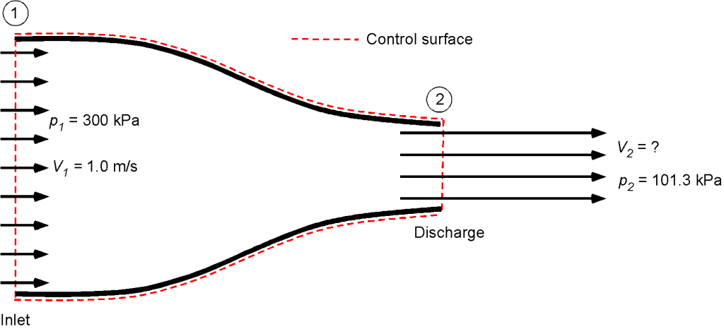

Using the Bernoulli equation ( $\varrho =$ constant) then

$p_1 + \frac{1}{2} \varrho V_1^2 = p_2 + \frac{1}{2} \varrho V_2^2$

Rearranging to solve for ${V_2}$ gives

$V_2 = \sqrt{ \frac{2 (p_1 - p_2)}{\varrho} + V_1^2} = \sqrt{ \frac{2 (300.0 - 101.3) \times 10^3}{1,000} + 1.0^2} = 19.96~\mbox{m/s}$

Worked Example #18

The airflow into a wind tunnel test section first passes through an upstream contraction section and then exhausts through a diffuser. Show by using the conservation equations that the flow velocity in the test section can be determined (calculated) by using the following:

(a) The difference between the total pressure in the opening (mouth) of the contraction section and the static pressure at the inlet to the test section.

(b) The difference in static pressure between the mouth of the contraction section and the static pressure at the inlet to the test section.

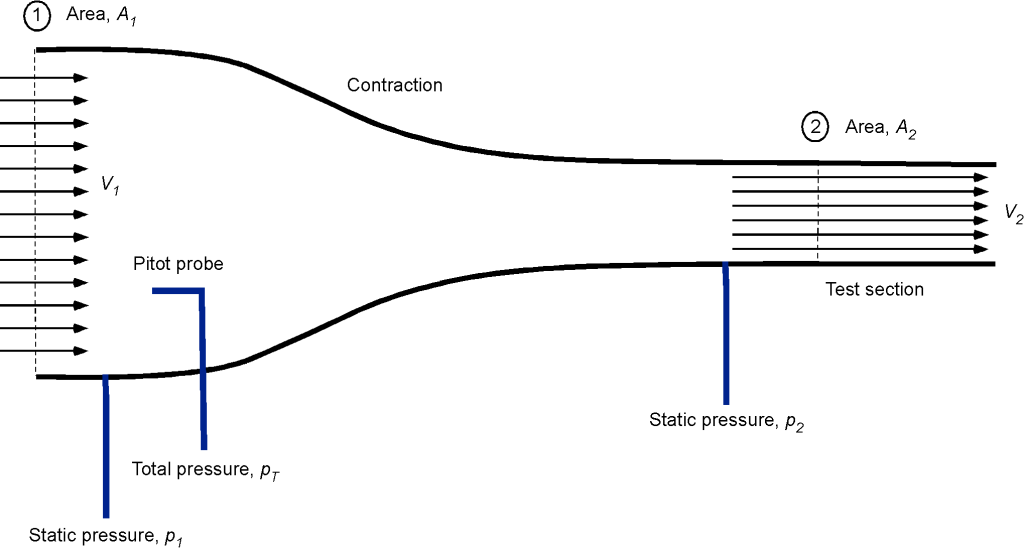
In each case, derive an equation relating the flow velocity in the test section to the pressure drop and the cross-sectional areas of the inlet and test sections.

The working part of a wind tunnel is a venturi. The airflow at the settling chamber (i.e., the mouth of the venturi) of area $A_1$ can be assumed to have a flow velocity ${V_1}$ with static pressure $p_1$ . The wind tunnel cross-section then contracts to a smaller area $A_2$ at the test section where the velocity has increased to ${V_2}$ , and the static pressure has decreased to $p_2$ . Notice that the velocity must increase if continuity (conservation of mass) is to be satisfied. A model (such as a wing or complete airplane model) is tested in the test section, and the aerodynamic characteristics are measured. The flow then passes downstream into a diverging duct called a diffuser.

First approach: From the continuity equation, the flow velocity in the test section will be

$\begin{equation*} V_2 = \left( \frac{A_1}{A_2} \right) V_1 \end{equation*}$

The pressures at the inlet (i.e., settling chamber) and the test section of the wind tunnel can be related to the flow velocities using Bernoulli’s equation, i.e.,

$\begin{equation*} p_1 + \frac{1}{2} \varrho V_1^2 = p_2 + \frac{1}{2} \varrho V_2^2 = p_T \end{equation*}$

where $p_T$ is the total pressure. This means that

$\begin{equation*} V_{2} = \sqrt{ \frac{2\left(p_T - p_{2}\right)}{\varrho} } \end{equation*}$

Therefore, the preceding equation can be used to determine the velocity in the test section from a measurement of total pressure measured in the contraction section (using a Pitot probe) and the static pressure at the test section (using static pressure taps). However, the density of the air must be known by measuring the temperature and pressure of the air in the flow and then calculating the density using the equation of state. This technique is used in many low-speed wind tunnels to measure the flow speed in the test section.

Second approach: From the continuity equation, the flow velocity in the test section will be

$\begin{equation*} V_2 = \left( \frac{A_1}{A_2} \right) V_1 \end{equation*}$

The static pressures at the inlet (i.e., settling chamber) and the test section of the wind tunnel can be related to the flow velocities using Bernoulli’s equation, i.e.,

$\begin{equation*} p_1 + \frac{1}{2} \varrho V_1^2 = p_2 + \frac{1}{2} \varrho V_2^2 \end{equation*}$

The velocity in the test section can be related to the static pressure drop across sections 1 and 2, i.e., the pressure drops $p_2 - p_1$ between the contraction and test sections. From the Bernoulli equation, we have

$\begin{equation*} V_2^2 = \frac{2}{\varrho} \left( p_2 - p_1 \right) + V_1^2 \end{equation*}$

This means that

$\begin{equation*} V_2^2 = \frac{2}{\varrho} \left( p_1 - p_2 \right) + \left( \frac{A_2}{A_1} \right)^2 V_2^2 \end{equation*}$

Solving for ${V_2}$ (the flow velocity in the test section), we obtain

$V_{2} = \sqrt{ \frac{2\left(p_{1} - p_{2}\right)}{\varrho\left[ 1 - \left(\displaystyle {\frac{A_{2}}{A_{1}} }\right)^{2} \right] } }$

In the second case, the area ratio $A_2/A_1$ must be known, but this is easily measured and is fixed for a given wind tunnel. Again, the density of the air must be known, and this is determined by measuring the temperature (using a thermocouple) and pressure (using a pressure transducer) of the air in the flow and then calculating the density using the equation of state. This technique is also used in low-speed wind tunnels to determine the flow speed in the test section, although it is a less common approach because, in practice, it is a little less accurate than the first method. The reason is that the static pressure drop $p_1 - p_2$ is much smaller than the difference between $p_T - p_2$ , so it is more difficult to accurately measure using a pressure transducer.

Worked Example #19

Consider the steady flow of a fluid element along a streamline, as shown in the figure below. By determining the net forces on the fluid element, show how the Bernoulli equation can be derived using Newton’s second law. Notice that $s$ is measured along the direction of the streamline.

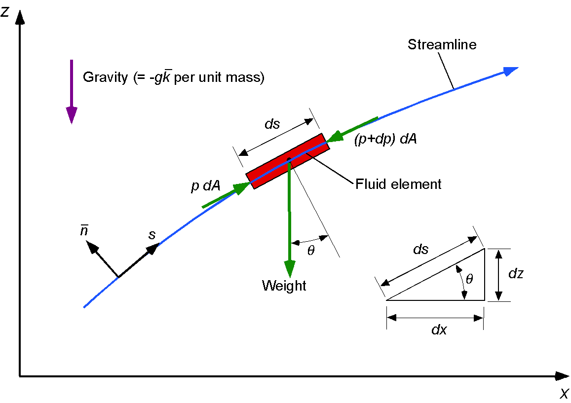
The forces acting on the fluid element in the $s$ -direction are the pressure and the component of the element’s weight, $W$ . Therefore, the net force on the element, $dF$ , is

$dF = p \, dA - (p + dp) \, dA - dW \sin \theta$

The weight of the element, $dW$ , is

$dW = \varrho (dA \, ds) \, g$

Therefore,

$dF = p \, dA - (p + dp) \, dA -\varrho (dA \, ds) \, g \, \sin \theta = - dp \, dA -\varrho (dA \, ds) \, g \, \sin \theta$

The acceleration of the fluid element is

$\frac{d V}{dt} = \frac{d V}{ds} \, \frac{d s}{dt} = V \, \frac{d V}{ds}$

where $V$ is the velocity of the fluid element along the streamline. Therefore, using Newton’s second law, then

$- dp \, dA -\varrho (dA \, ds) \, g \, \sin \theta = \left( \frac{dW}{g} \right) V \, \frac{d V}{ds} = \varrho (dA \, ds) \, V \, \frac{d V}{ds}$

or

$- dp \, dA -\varrho (dA \, ds) \, g \, \frac{dz}{ds} = \varrho (dA \, ds) \, V \, \frac{d V}{ds}$

noting that $\sin \theta = dz/ds$ . After rearrangement, then

$- dp \, dA -\varrho \, g \, dA \, dz = \varrho dA \, ds \, V \, \frac{d V}{ds}$

Dividing through by $dA$ gives

$-dp -\varrho \, g \, dz = \varrho \, V \, dV = \frac{1}{2} \varrho \, d(V^2)$

or

$dp + \varrho \, g \, dz + \frac{1}{2} \varrho \, d(V^2) = 0$

Finally, after integration, then

$p + \varrho \, g \, z + \frac{1}{2} \varrho \, V^2 = \mbox{constant}$

which again is the Bernoulli equation.

Worked Example #20

A horizontal water jet with a diameter ${d}$ = 4 cm impacts a vertical plate at a velocity of 10 m/s. Draw an appropriate sketch and control volume to analyze this problem. Using the conservation laws of fluid dynamics, find the force on the plate, $F$ . Make a one-dimensional, steady flow assumption.

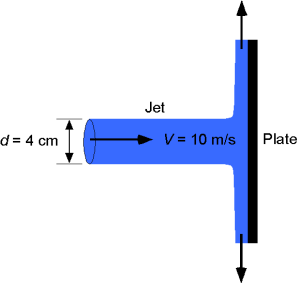
The mass flow rate in the jet is

$\overbigdot{m_j} = \varrho V_j A_j$

where $V_j$ = 10 m/s and $A_j = \pi d_j^2/4 = \pi (0.04)^2/4$ = 0.00126 m ${^{2}}$ .

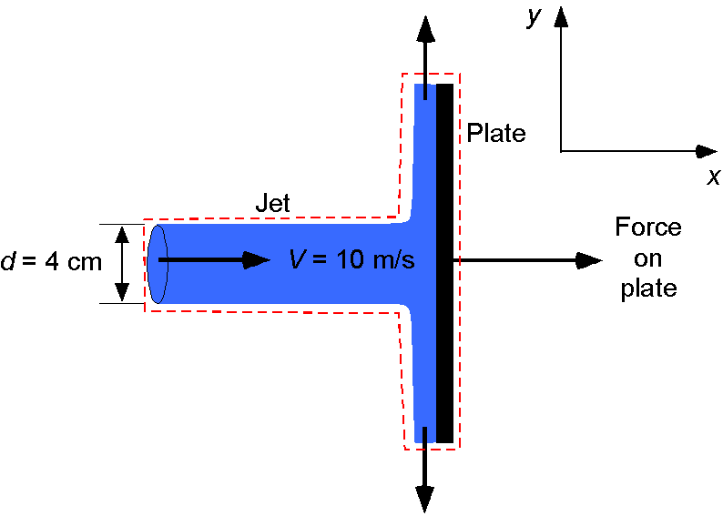
The horizontal jet hits the plate and is brought to rest horizontally. To do this, the force on the fluid has to be equal to the time rate of change of momentum in that direction, and the force on the plate is in the opposite direction, i.e.,

$F = \overbigdot{m_j} V_j = (\varrho V_j A_j) V_j = \varrho A_j V_j^2$

Substituting the numerical values gives

$F = \varrho A_j V_j^2 = (1,000) (0.00126) 10^2 = 125.66~\mbox{N}$

Worked Example #21

An incompressible gas flow in an exhaust system encounters a change in the size of the exhaust pipe as it transitions to the muffler. The exit diameter of the muffler pipe is $D_2$ = 4.1 inches, and the diameter of the inlet header pipe is $D_1$ = 2.2 inches. The exhaust gas is discharged at a speed of ${V_2}$ = 14.3 ft/s. If the static pressure difference between the header and the muffler is measured using a U-tube water manometer, then calculate the height ${h}$ between the two columns. Assume 1-dimensional flow and no losses. Also assume that $\varrho_{w} = 1.94$ slug/ft ${^3}$ and $\varrho_{\rm gas} = 0.0023$ slug/ft ${^3}$ .

Assuming steady, 1-dimensional flow, applying the continuity equation between the inlet (section 1) and the exit (section 2) gives

$\varrho_1 \, A_1\, V_1 = \varrho_2 \, A_2 \, V_2$

And because $\varrho_1 = \varrho_2 = \varrho =$ constant in this case (the flow is stated to be incompressible), then

$A_1 \, V_1 = A_2 \, V_2$

Therefore, solving for the inlet velocity ${V_1}$ gives

$V_1 = \frac{A_2 \, V_2}{A_1} = \frac{\left(\displaystyle{\frac{\pi}{4}}\right)D_2^2 \, V_2}{\left(\displaystyle{\frac{\pi}{4}}\right)D_1^2} = \frac{\left(\displaystyle{\frac{4.1}{12}}\right)^2 \times 14.3 }{\left(\displaystyle{\frac{2.2}{12}} \right)^2} = \frac{4.1^2 \times 14.3 }{2.2^2} = 49.67 \mbox{ ft/s}$

The application of Bernoulli’s equation gives

${ p_1 + \frac{1}{2} \, \varrho_{\rm gas}\, V_1^2 + \varrho_{\rm gas} \, g \, z_1 = p_2 + \frac{1}{2} \, \varrho_{\rm gas} \, V_2^2 + \varrho_{\rm gas} \, g \, z_2 }$

There is no change in the vertical height of the mean flow in this case, so $z_1 = z_2 = 0$ and

$p_1 + \frac{1}{2} \, \varrho_{\rm gas}\, V_1^2 = p_2 + \frac{1}{2} \, \varrho_{\rm gas} \, V_2^2$

Rearranging for the pressure difference $p_2 - p_1$ gives

$p_2 - p_1 = \frac{1}{2}\varrho_{\rm gas}\left(V_1^2 - V_2^2\right)$

The U-tube manometer, as shown, will measure this static pressure difference $p_2 - p_1$ , so using the hydrostatic equation, the pressure difference is

$p_2 - p_1 = \varrho_{w} \, g \, h$

making sure we use the density of water here. Therefore, equating the latter two equations gives

$\varrho_{w} \, g \, h = \frac{1}{2}\varrho_{\rm gas}\left(V_1^2 - V_2^2\right)$

and solving for ${h}$ leads to

$h = \frac{\varrho_{\rm gas}}{2 \, \varrho_{w} \, g}\left(V_1^2 - V_2^2\right) = \frac{0.0023}{2 \times 1.94 \times 32.17}\left( 49.67^2 - 14.3^2\right) = 0.0417~\mbox{ft} = 0.5~\mbox{inches}$

Worked Example #22

Gas flows at speed ${V_2}$ through a horizontal section of pipe whose cross-sectional area is $A_2 = 0.0700$ m ${^{2}}$ . The gas has a density of $\varrho = 1.34$ kg/m ${^3}$ . A venturi meter with a cross-sectional area of $A_1 = 0.0500$ m ${^{2}}$ has been substituted for a section of the larger pipe. The pressure difference between the two sections is $p_2 - p_1 = 120.1$ Pa. Find: (a) Find the speed ${V_2}$ of the gas in the original pipe. (b) Find the speed ${V_1}$ in the throat of the venturi. (c) Find the volume flow rate $Q$ .

(a) We are told the gas has a density of 1.34 kg/m ${^3}$ , implying constant density so that the Bernoulli equation can be used, i.e.,

$p_1 + \frac{1}{2} \varrho V_1^2 + \varrho g z_1 = p_2 + \frac{1}{2} \varrho V_2^2 + \varrho g z_2$

We can assume from the figure that both pressure gages are at the same height, so $z_1 = z_2$ , so the Bernoulli equation is now

$p_1 + \frac{1}{2} \varrho V_1^2 = p_2 + \frac{1}{2} \varrho V_2^2$

The continuity equation (constant density gas) is

$V_1 A_1 = V_2 A_2$

so

$V_1 = V_2 \left( \frac{ A_2}{A_1} \right)$

The Bernoulli equation becomes

$p_1- p_2 = \frac{1}{2} \varrho \left( V_2^2 - V_1^2 \right) = \frac{1}{2} \varrho V_2^2 \left( 1 - \left( \frac{A_2}{A_1} \right)^2 \right)$

We are given that $A_1 = 0.05$ m ${^{2}}$ and $A_2 = 0.07$ m ${^{2}}$ so ${V_2}$ becomes

$V_2 = \sqrt{ \frac{ 2(p_1 - p_2) }{\varrho \left( \left( 1- \displaystyle{\frac{A_2}{A_1}} \right)^2 \right) }} = \sqrt{ \frac{ 2 \times (-120.1)}{1.34 \left( 1 -\left( \displaystyle{\frac{0.07}{0.05}} \right)^2 \right) }} = 13.67~\mbox{m/s}$

(b) Using the continuity equation, then

$V_1= V_2 \left( \frac{ A_2}{A_1} \right) = 13.67 \left( \frac{ 0.07}{0.05} \right) = 19.14~\mbox{m/s}$

(c) The volume flow rate $Q$ is

$Q = A_1 V_1 (= A_2 V_2)$

so we get

$Q =A_1 V_1 = 0.05 \times 19.14 = 0.957~\mbox{m${^3}$/s}$

Worked Example #23

Water ( $\varrho$ = 1,000 kg/m ${^3}$ ) flows in a hose with a velocity of 1.0 m/s and a pressure of 300 kPa. At the nozzle, the pressure decreases to atmospheric (101.3 kPa). There is no change in height. (a) Use the Bernoulli equation to calculate the velocity of the water exiting the nozzle. (b) The hose ejects the water stream through the nozzle with a final diameter of 3 cm. The stream is then directed onto a stationary wall. Determine the force on the wall from the stream.

(a) We are told to use the Bernoulli equation ( $\varrho =$ constant), which is

$p_1 + \frac{1}{2} \varrho V_1^2 = p_2 + \frac{1}{2} \varrho V_2^2$

Rearranging to solve for ${V_2}$ gives

$V_2 = \sqrt{ \frac{2 (p_1 - p_2)}{\varrho} + V_1^2} = \sqrt{ \frac{2 (300.0 - 101.3) \times 10^3}{1,000} + 1.0^2} = 19.96~\mbox{m/s}$

(b) The need for a force suggests using the momentum equation. The momentum of the jet before the wall is $\overbigdot{m} V_2$ where

$\overbigdot{m} = \varrho A_2 V_2$

When the jet hits the wall, it is brought to rest in the horizontal direction (it will be deflected in all other directions)

$\overbigdot{m} = \varrho A_2 V_2^2 - 0 = F$

where $F$ is the force. Solving for $F$ gives

$F = \varrho A_2 V_2^2 = \varrho \left( \frac{\pi d^2}{4} \right) V_2^2 = 1,000 \left( \frac{\pi \, 0.03^2}{4} \right) 19.96^2 = 281.6~\mbox{N}$

Worked Example #24

Water flows through a converging nozzle. If the pressure at point A at the intake to the nozzle is 19.7 lb/in ${^{2}}$ , then determine the height ${h}$ shown on the U-tube manometer. Notes: Assume atmospheric pressure $p_a$ is 14.7 lb/in ${^{2}}$ . The density of water can be assumed to be 1.93 slugs/ft ${^3}$ , and the specific gravity of mercury is 13.6.

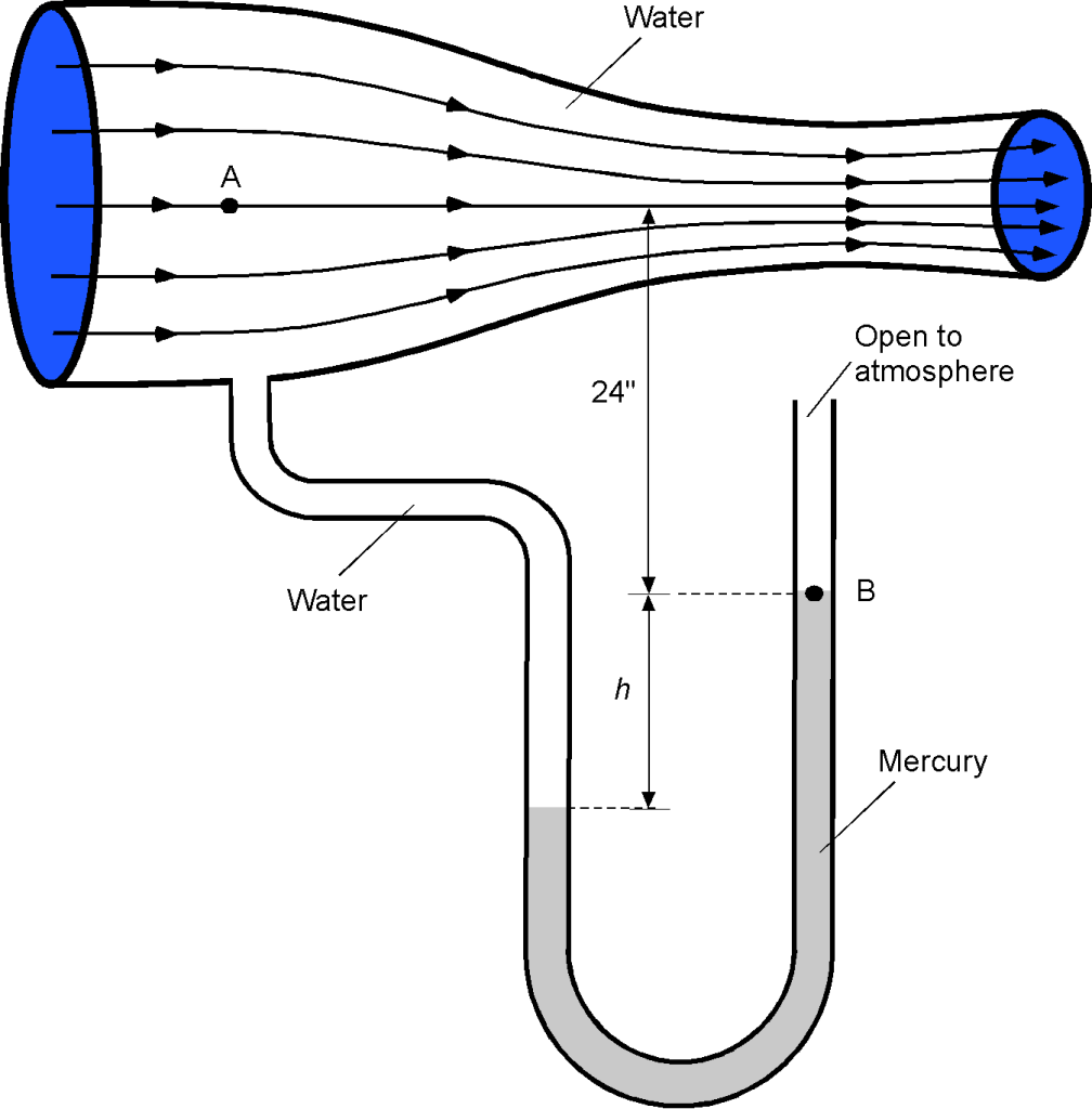
Let the height from point A to point B be $h_1$ . Let $h_2$ be the height from the bottom of the U-tube to the lowest point of the mercury. Considering the left leg of the U-tube, the pressure at the lowest point in the U-tube will be

$p = p_A + \varrho_{w} \, g h_1 + \varrho_{w} \, g h + \varrho_{\rm Hg} \, g h_2$

For the right leg, the pressure at the same point will be

$p = p_a + \varrho_{\rm Hg} \, g h + \varrho_{\rm Hg} \, g h_2$

Equating these latter two equations gives

$p_A + \varrho_{w} \, g h_1 + \varrho_{w} \, g h = p_a + \varrho_{\rm Hg} \, g h$

and rearranging gives

$\left( \varrho_{\rm Hg} - \varrho_{w} \right) g h = \left( p_A - p_a \right) + \varrho_{w} \, g h_1$

Solving for ${h}$ gives

$h = \frac{\left( p_A - p_a \right) + \varrho_{w} \, g h_1}{\left( \varrho_{\rm Hg} - \varrho_{w} \right) g}$

Now, we can substitute the information given. Notice that $p_A - p_a$ = 5 lb/in ${^{2}}$ = (5 $\times$ 144) lb/ft ${^{2}}$ = 720.0 lb/ft ${^{2}}$ . Therefore,

$h = \frac{720.0 + 1.93 \times 32.17 \times (24.0/12) }{(13.6 - 1) \times 1.93 \times 32.17} = 1.079~\mbox{ft} = 12.94~\mbox{inches}$

Worked Example #25

Water flows through a pipe of circular cross-section with a volume flow rate of 14.2 ft ${^3}$ /s encounters a change in the area and height of the pipe as it passes through an elbow-type of coupling. The exit area of the pipe is $A_2$ = 2.4 ft ${^{2}}$ , and the area of the inlet is $A_1$ = 4.8 ft ${^{2}}$ . Assume 1-dimensional flow and no losses with $\varrho_{w} = 1.94$ slug/ft ${^3}$ . (a) Determine the flow velocities at the entrance ( ${V_1}$ ) and the exit ( ${V_2}$ ) in units of ft/s. (b) If ${z_1}$ = 6 inches and ${z_2}$ = 25 inches, what is the static pressure difference between the inlet and outlet, i.e., the value of $p_1 - p_2$ , in units of lb/in ${^{2}}$ .

(a) The fluid is water, so it is incompressible. The application of the continuity equation in one-dimensional form gives

$V_1 \, A_ 1 = A_ 2 V_2 = Q = \mbox{constant}$

Therefore, the inlet flow velocity ${V_1}$ is

$V_1 = \frac{Q}{A_1} = \frac{14.2}{4.8} = 2.96~\mbox{ft/s}$

and for the outlet flow velocity ${V_2}$ , then we know that

$V_1 \, A_ 1 = A_ 2 V_2$

so

$V_2 = \left( \frac{A_2}{A_1} \right) V_1 = \left( \frac{4.8}{2.4} \right) V_1 = 2 \, V_1 = 5.92~\mbox{ft/s}$

It will also be noted that

$V_2 = \frac{Q}{A_2} = \frac{14.2}{2.4} = 5.92~\mbox{ft/s}$

(b) The Bernoulli equation is

$p + \frac{1}{2} \varrho \, V^2 + \varrho g z = \mbox{constant}$

so, in this case

$p_1 + \frac{1}{2} \varrho_{w} \, V_1^2 + \varrho_{w} \, g \, z_1 = p_2 + \frac{1}{2} \varrho_{w} \, V_2^2 + \varrho_{w} \, g \, z_2$

We are asked for the pressure difference $p_1 - p_2$ , so using the Bernoulli equation gives

$p_1 - p_2 = \frac{1}{2} \varrho_{w} \left( V_2^2 - V_1^2 \right) + \varrho_{w} \, g \left( z_2 - z_1 \right)$

and substituting the known values gives

$p_1 - p_2 = \frac{1}{2} \times 1.94 \left( 5.92^2 - 2.96^2 \right) + 1.94 \times 32.17 \times \left( 25.0 - 6.0 \right)/12~\mbox{lb/ft${^{2}}$}$

Notice that it is necessary to convert the hydrostatic head (last term) from units of inches to feet to keep the entire equation in consistent base units of lb, ft, and seconds (s). Evaluating the arithmetic gives

$p_1 - p_2 = 124.31~\mbox{lb/ft${^{2}}$} = 124.31/144 ~\mbox{lb/in${^{2}}$} = 0.863~\mbox{lb/in${^{2}}$}$

noting that 144 lb/in ${^{2}}$ is equal to 1 lb/ft ${^{2}}$ .

Worked Example #26

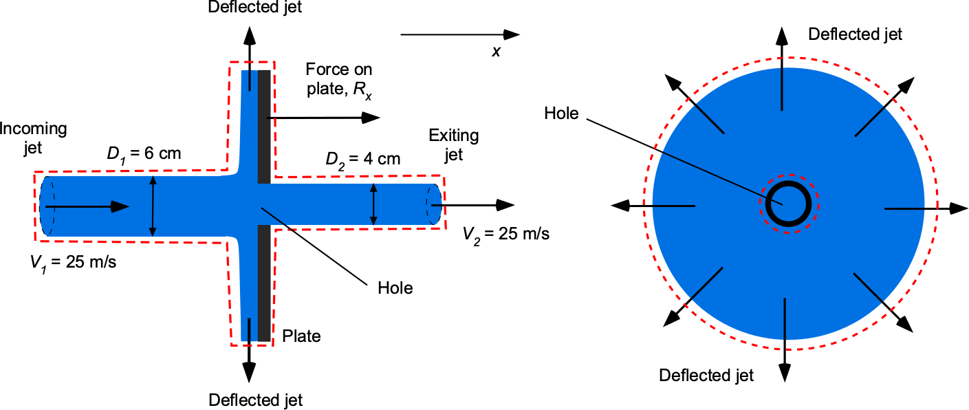
As shown in the figure below, a 6 cm diameter water jet strikes a circular flat plate containing a hole with a diameter of 4 cm. Part of the jet passes through the hole, and the other part is deflected radially symmetrically away from the plate. The density of water can be assumed to be 998.23 kg m ${^{-3}}$ . (a) Calculate the mass flow rate of the jet toward the plate. (b) Calculate the mass flow rate of the jet’s deflected part. (c) Determine the magnitude and direction of the force required to hold the plate stationary.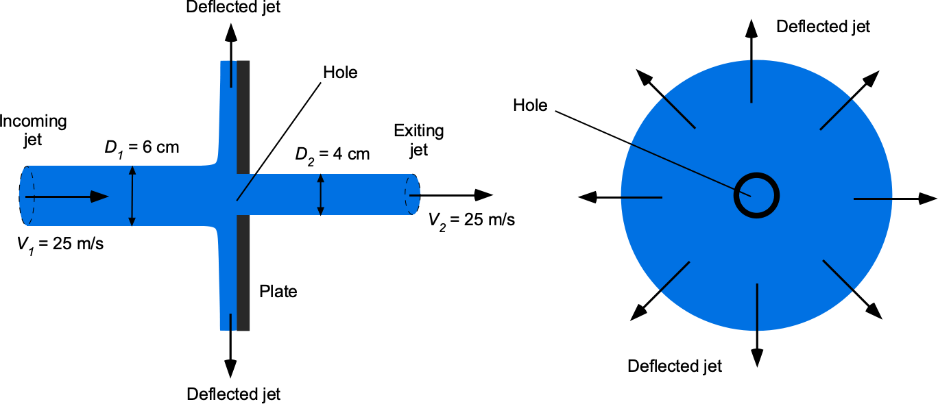

(a) Valid assumptions are incompressible, steady, no body force, inviscid, and one-dimensional flow across any given cross-section. The control surface is shown in the figure below.

The mass flow rate of the jet toward the plate is

$\overbigdot{m}_1 = \varrho \, V_1 \, A_1$

and inserting the values gives

$\overbigdot{m}_1 = 998.23\times 25.0 \times(\pi/4)\times(0.06)^2 = 70.56~\mbox{kg/s}$

(b) Conservation of mass in the one-dimensional form gives

$\varrho \, (-V_1) \, A_1 + \varrho \, V_2 \, A_2 + \varrho\, V_3 \, A_3 = 0$

with the minus sign on the first term indicating that the flow is inward and in the opposite direction to the outward-pointing surface normal vector. In terms of mass flow rates, then

$-\overbigdot{m}_1 + \overbigdot{m}_2 + \overbigdot{m}_3 = 0$

Therefore, the radially deflected mass flow rate is

$\overbigdot{m}_3 = \overbigdot{m}_1 - \overbigdot{m}_2$

Inserting the numerical values gives

$\overbigdot{m}_3 = 998.23 \times 25.0 \times \pi/4 \times \left( 0.06^2 - 0.04^2 \right) = 39.2~\mbox{kg s$^{-1}$}$

(c) The entire system is subjected to a background (atmospheric) pressure, so no net pressure force is acting on the control volume. The force on the fluid (to change its momentum) is found from the conservation of momentum. Only the the part of the mass flow $\overbigdot{m}_3$ is deflected, so

$F_x =\underbrace{\overbigdot{m}_3 \, V_x ( = 0) }_{\begin{tabular}{c} \scriptsize Zero momentum \\[-3pt] \scriptsize out in the \\[-3pt] \scriptsize ${x}$ direction \end{tabular}} - \underbrace{\overbigdot{m}_3 \, V_1}_{\begin{tabular}{c} \scriptsize Deflected part \\[-3pt] \scriptsize of incoming \\[-3pt] \scriptsize jet in the \\[-3pt] \scriptsize ${x}$ direction \end{tabular}}$

It is unnecessary to determine the radial velocity. Inserting the numbers gives

$F_x = -39.2 \times 25.0 = -980.01~\mbox{N}$

Therefore, the force applied to the plate by the water jet is

$R_x = 980.01~\mbox{N}$

A force of $-980.01$ N is required to hold the plate stationary, i.e., a minus sign, so the force acts to the left.

Worked Example #27

Two plates, set 4 cm apart, are separated by an oil bed. The bottom plate is stationary, but the top plate moves at a speed of 3.5 m/s. Calculate the shear stress in the oil. Assume that the oil’s dynamic viscosity coefficient is 583.95 Pa s. Note: Pa s is an SI unit of viscosity and is equivalent to Newton-second per square meter (N s m $^{-2}$ ), which is sometimes referred to as the Poiseuille (Pl).

It is necessary to calculate the shear stress in a fluid, $\tau$ , based on the formation of a velocity gradient. The use of Newton’s formula of viscosity gives

$\tau = \mu \left( \frac{du}{dy} \right)$

Newtonian flow will give a constant uniform velocity gradient, in this case, between the upper and lower plates will be

$\frac{du}{dy} = \frac{3.4}{0.04} = 87.5 \mbox{ s$^{-1}$}$

This means that the shear stress per unit depth in the fluid will be

$\tau = \mu \left( \frac{du}{dy} \right) = 51.1 \mbox{ kPa}$

Worked Example #28

Water ( $\varrho_w$ = 1.94 slug ft ${^{-3}}$ ) flows at a mass flow rate of $\overbigdot{m}$ = 6.0 slug s $^{-1}$ through a nozzle with an entrance diameter $d_e = 10.0$ in and and exit diameter of $d_j = 4.0$ . The water hits an angled bracket, as shown in the figure below, such that exactly half of the mass flow rate of the stream deflects to the left and half deflects to the right. The diameter of the deflected jets, $d_d$ , is 1.3 in. Assume that the water all stays in a horizontal plane and one-dimensional flow.
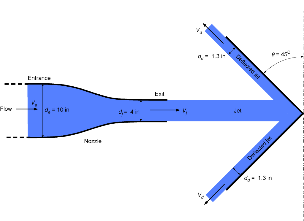
Calculate the following:

The velocity of the water entering and exiting the nozzle, $V_e$ and $V_j$ .
The change in pressure $\Delta p$ between the nozzle entrance and its exit.
The velocity $V_d$ of the water in the deflected jets.
The magnitude and direction of the force on the bracket.

1. The velocity of the water entering and exiting the nozzle can be determined using conservation of mass (continuity equation), i.e.,

$\overbigdot{m} = \varrho_w \, A_e \, V_e = \varrho_w \, A_j \, V_j$

The entrance area $A_e$ is

$A_e = \frac{\pi d_e^2}{4} = \frac{\pi (10.0/12.0)^2}{4} = 0.5454~\mbox{ft${^{2}}$}$

The entrance velocity is

$V_e = \frac{\overbigdot{m}}{ \varrho_w \, A_j}$

and substituting the values gives

$V_e = \frac{6.0}{1.94 \times 0.5454} = 5.67~\mbox{ft s$^{-1}$}$

The exit jet area $A_j$ is

$A_j = \frac{\pi d^2}{4} = \frac{\pi (4.0/12.)^2}{4} = 0.0873~\mbox{ft${^{2}}$}$

The exit jet velocity is

$V_j = \frac{\overbigdot{m}}{ \varrho_w \, A_j}$

and substituting the values gives

$V_j = \frac{6.0}{1.94 \times 0.0873} = 35.43~\mbox{ft s$^{-1}$}$

2. The change in pressure $\Delta p$ between the nozzle inlet and its exit can be found using the Bernoulli equation, i.e.,

$p + \frac{1}{2} \varrho \, V^2 = \mbox{constant}$

In this case, then

$p_e + \frac{1}{2} \varrho V_e^2 = p_j + \frac{1}{2} \varrho V_j^2$

We are asked for a change in pressure, so

$p_e - p_j = \Delta p = \frac{1}{2} \varrho \left( V_j^2 - V_e^2 \right)$

and substituting the values gives

$\Delta p = 0.5 \times 1.94 \times \left( 35.43^2 - 5.67^2 \right) = 1,186.44~\mbox{lb ft$^{-2}$}$

3. The velocity ${V_2}$ of the water in the deflected jet can be found using continuity. In this case, half of the mass flow is deflected in each direction, so

$\frac{\overbigdot{m}}{2} = \varrho_w \, A_d \, V_d$

The deflected jet area $A_j$ is

$A_d = \frac{\pi d_d^2}{4} = \frac{\pi (1.3/12.0)^2}{4} = 0.00922~\mbox{ft${^{2}}$}$

The deflected jet velocity is

$V_d = \frac{\overbigdot{m}}{ 2 \varrho_w \, A_d}$

and substituting the values gives

$V_d = \frac{6.0}{2 \times 1.94 \times 0.00922} = 167.72~\mbox{ft s$^{-1}$}$

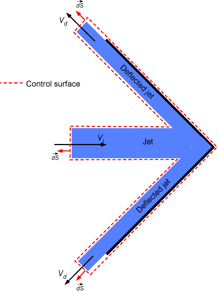
4. The force of the plate from the water can be determined from the time rate of change of momentum of the fluid, a suitable control volume being shown below. To this end, the rate of momentum of the water coming onto the deflector in the downstream (horizontal) direction is $\overbigdot{m} V_j$ . Likewise, the rate of deflected momentum coming out away from the defector is $-\overbigdot{m} V_d \, \cos 45^{\circ}$ . Notice that the $\cos 45^{\circ}$ term gives the correct horizontal momentum component.

Therefore, the force on the plate will be the time rate of the net momentum so that

$F = \overbigdot{m} V_j - (- \overbigdot{m} V_d \, \cos (45^{\circ}) = \overbigdot{m} V_j + \overbigdot{m} V_d \, \cos (45^{\circ}) = \overbigdot{m} \left( V_j + V_d \, \cos (45^{\circ} \right)$

Inserting the numbers gives

$F = \overbigdot{m} \left( V_j + V_d \, \cos 45^{\circ} \right) = 6.0 \times \left(35.43 +167.72 \times 0.707 \right) = 924.16~\mbox{lb}$

which will be applied by the water in the downstream direction, away from the nozzle

Worked Example #29

Consider the steady flow of a liquid through an elbow-shaped converging axisymmetric pipe joint with an inlet area $A_1$ and outlet area $A_2$ , as shown in the figure below. The volumetric flow rate is $Q$ . The elbow angle is $\theta$ in a horizontal plane. Assume that the flow inside the pipe is one-dimensional. Use the continuity and momentum equations to set up the procedure to find the resultant force on the pipe. Note: You do not have to find the force; show how to use and set up the relevant equations.

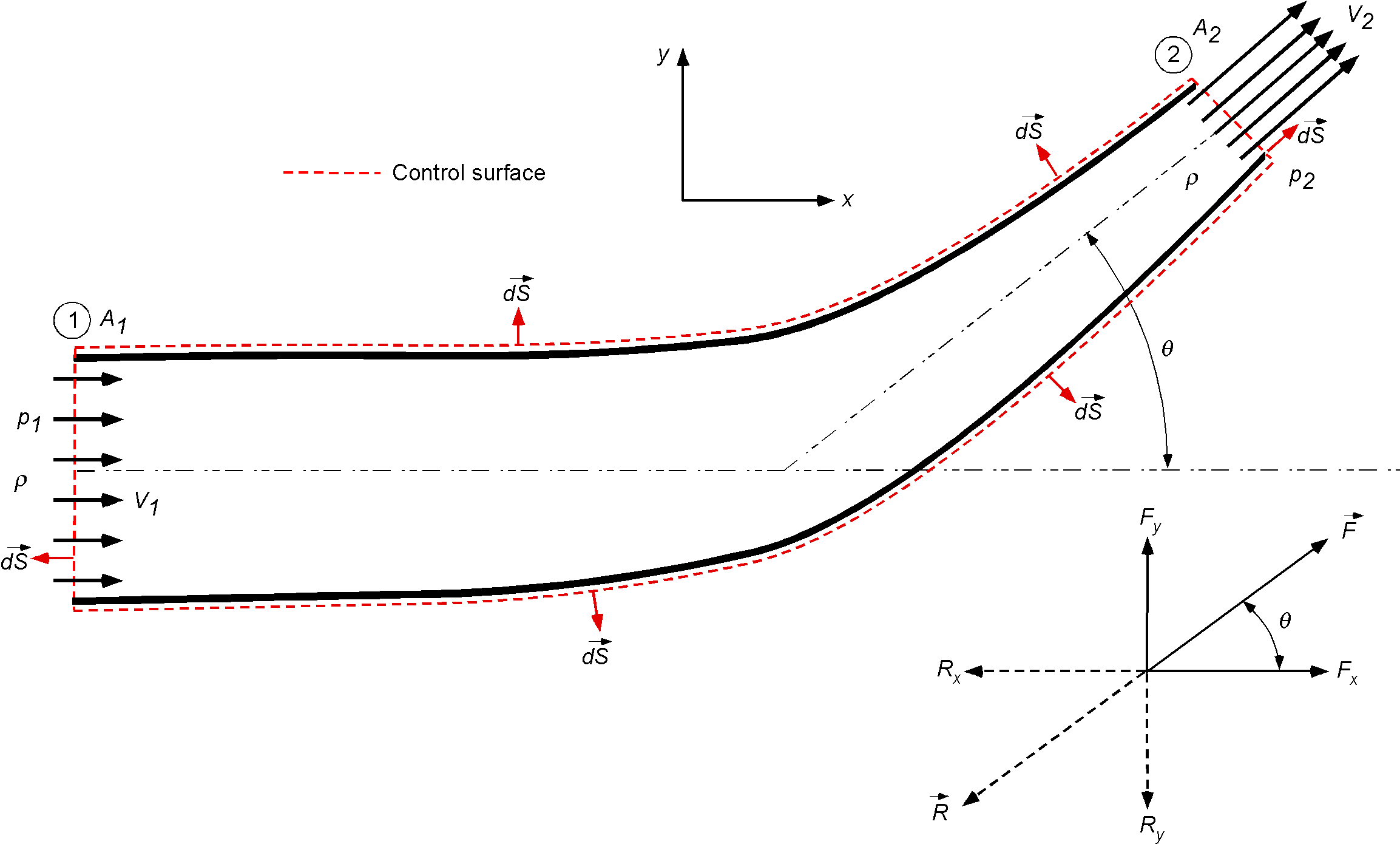
The flow is steady, so ${\partial/\partial t \equiv 0}$ , and the flow can be assumed as inviscid, so $\vec{F}_{\mu} = 0$ . The fluid is a liquid (which has a relatively high density), but there is no change in elevation from one side of the nozzle to the other. Therefore, gravitational effects can be neglected.

The general form of the momentum equation is

$\oiiint_{\cal{V}} \varrho \vec{F} _b d{\cal{V}} -\oiint_S p \, d\vec{S} + \vec{F}_{\mu} = \frac{\partial}{\partial t}\oiiint_{\cal{V}} \varrho \, \vec{V} d {\cal{V}} + \oiint_S (\varrho \, \vec{V} \bigcdot d\vec{S}) \vec{V}$

and the reduced form for the assumptions made in this question leads to

$- \oiint_S p \, d\vec{S} = \oiint_S (\varrho \, \vec{V} \bigcdot d\vec{S}) \vec{V}$

The pressure integral on the left-hand side can be written as

$\oiint_S p \, d\vec{S} = \iint_{A_1} p \, d\vec{S} + \iint_{A_2} p \, d\vec{S} + \iint_{\rm Walls} p \, d\vec{S}$

In this case, the force of the walls on the fluid, say $\vec{F}$ (to change its momentum), needs to be determined, i.e., this is the unknown. There is also an equal and opposite force on the nozzle, say $\vec{R}$ , which ultimately is the force to be determined.

We are told to assume one-dimensional over the cross-section of the nozzle, but the flow moves in two directions in this case, ${x}$ and ${y}$ . Therefore, two scalar momentum equations will be in the ${x}$ and ${y}$ directions, respectively. In general form, the momentum equation is

$-\oiint_S p \, d\vec{S} = - \vec{F} - \iint_{A_1} p \, d\vec{S} - \iint_{A_2} p \, d\vec{S} = \oiint_S (\varrho \, \vec{V} \bigcdot d\vec{S}) \vec{V}$

With the one-dimensional assumption, then for the ${x}$ direction, then

$-F_{x} - p_1 A_1 + p_2 A_2 \cos \theta = (\varrho_2 A_2 V_2) V_2 \cos \theta - \varrho_1 A_1 V_1 ^2$

so that

$F_{x} = (p_2 A_2 \cos \theta - p_1 A_1) + \varrho_2 A_2 V_2^2 \cos \theta - \varrho_1 A_1 V_1^2$

For the momentum equation in the ${y}$ direction, then

$-F_{y} - 0 - p_2 A_2 \sin \theta = (\varrho_2 A_2 V_2) V_2 \sin \theta - 0$

so that

$F_{y} = p_2 A_2 \sin \theta + \varrho_2 A_2 V_2^2 \sin \theta$

We are not asked to move forward from this point, just to set up the equations to be solved. In summary, these are

$F_{x} = (p_2 A_2 \cos \theta - p_1 A_1) + \varrho_2 A_2 V_2^2 \cos \theta - \varrho_1 A_1 V_1^2$

and

$F_{y} = p_2 A_2 \sin \theta + \varrho_2 A_2 V_2^2 \sin \theta$

We also have the continuity equation to round out the other two equations, i.e.,

$Q = A_1 V_1 = A_2 V_2$

Worked Example #30

Water flows through a pipe of circular cross-section and encounters a change in the area of the pipe as it passes through an elbow-type of coupling, as shown in the figure below. The pipe is in a horizontal plane, i.e., the ${x}$ – ${y}$ plane. The volume flow rate is 13.4 ft ${^{3}}$ /s. The exit area of the pipe is $A_2$ = 2.1 ft ${^{2}}$ , and the area of the inlet is $A_1$ = 4.8 ft ${^{2}}$ . Assume uniform flow properties across any cross-section and no losses. For water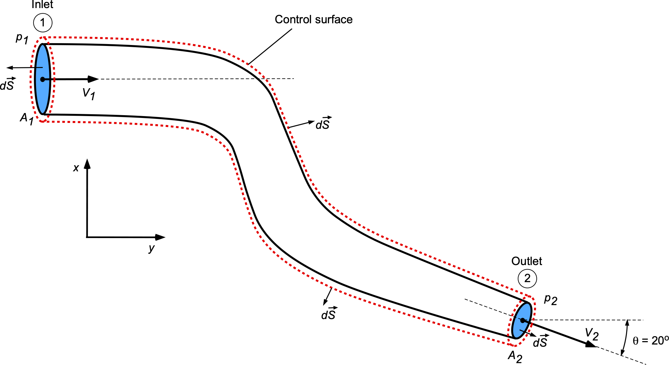, $\varrho_{w} = 1.94$ slug/ft ${^{3}}$ .

Determine the entrance velocity ( ${V_1}$ ) and the exit velocity ( ${V_2}$ ) in units of ft/s.
What is the static pressure difference between the outlet and inlet, i.e., the value of $p_2 - p_1$ , in units of lb/in ${^{2}}$ ?
Determine the equation(s) for the force on the pipe.

1. The flow rate and the input and output areas are given, so

$V_1= \left( \dfrac{Q}{A_1} \right) = \dfrac{13.4}{4.8} = 2.79~\mbox{ft/s}$

and

$V_2 = \left( \dfrac{Q}{A_2} \right) = \dfrac{13.4}{2.1} = 6.38~\mbox{ft/s}$

2. The Bernoulli equation is

$p_1 + \frac{1}{2} \varrho_w V_1^2 + \varrho_w g z_1 = p_2 + \frac{1}{2} \varrho_w V_2^2 + \varrho_w g z_2$

The flow is in the $x-y$ plane so there is no hydrostatic head, i.e., $z_1 = z_2 = 0$ , so

$p_1 + \frac{1}{2} \varrho_w V_1^2 = p_2 + \frac{1}{2} \varrho_w V_2^2$

Rearranging to solve for static pressure difference between the inlet and outlet gives

$p_2 - p_1 = \frac{1}{2} \varrho_w \left( V_1^2 - V_2^2 \right)$

Substituting the known values gives

$p_2 - p_1 = \frac{1}{2} \times 1.94 \left( 2.79^2 - 6.38^2 \right) = -31.93~\mbox{lb/ft${^{2}}$}$

We are asked for the pressure in units of lb/in ${^{2}}$ , so

$p_2 - p_1 = -31.93~\mbox{lb/ft${^{2}}$} = \dfrac{-31.93}{144} = -0.222~\mbox{lb/in${^{2}}$}$

3. The force on the pipe can be obtained by assessing the net pressure forces and the time rate of change of momentum. The momentum equation in terms of the two scalar components will be

$F_{x} + (p_1 A_1 - p_2 A_2 \cos \theta) = \overbigdot{m} \, V_2 \cos \theta - \overbigdot{m} \, V_1$

and

$F_{y} + (0 - p_2 A_2 \sin \theta) = \overbigdot{m} \, V_2 \sin \theta - 0$

where $F_x$ and $F_y$ are the forces on the fluid in the ${x}$ and ${y}$ directions, respectively.

Rearranging the ${x}$ -momentum equation gives

$F_x = \varrho_w A_1 V_1 \left( V_2 \cos \theta - V_1 \right) - \left( p_1 A_1 - p_2 A_2 \cos \theta \right)$

and for $F_y$ , then

$F_y = \varrho_w A_1 V_1 V_2 \sin \theta + p_2 A_2 \sin \theta$

Worked Example #31

Water ( $\varrho_w = 1,000 \, \text{kg/m}^3$ ) flows at a mass flow rate of $\dot{m} = 6.0 \, \text{kg/s}$ through a nozzle with an entrance diameter $d_e = 10.0 \, \text{cm}$ and an exit diameter $d_j = 4.0 \, \text{cm}$ . The water then hits a curved bracket, as shown in the figure below. The diameter of the deflected jet is $d_d = 3.0 \, \text{cm}$ . Assume the water stays in a horizontal plane and is a one-dimensional flow.

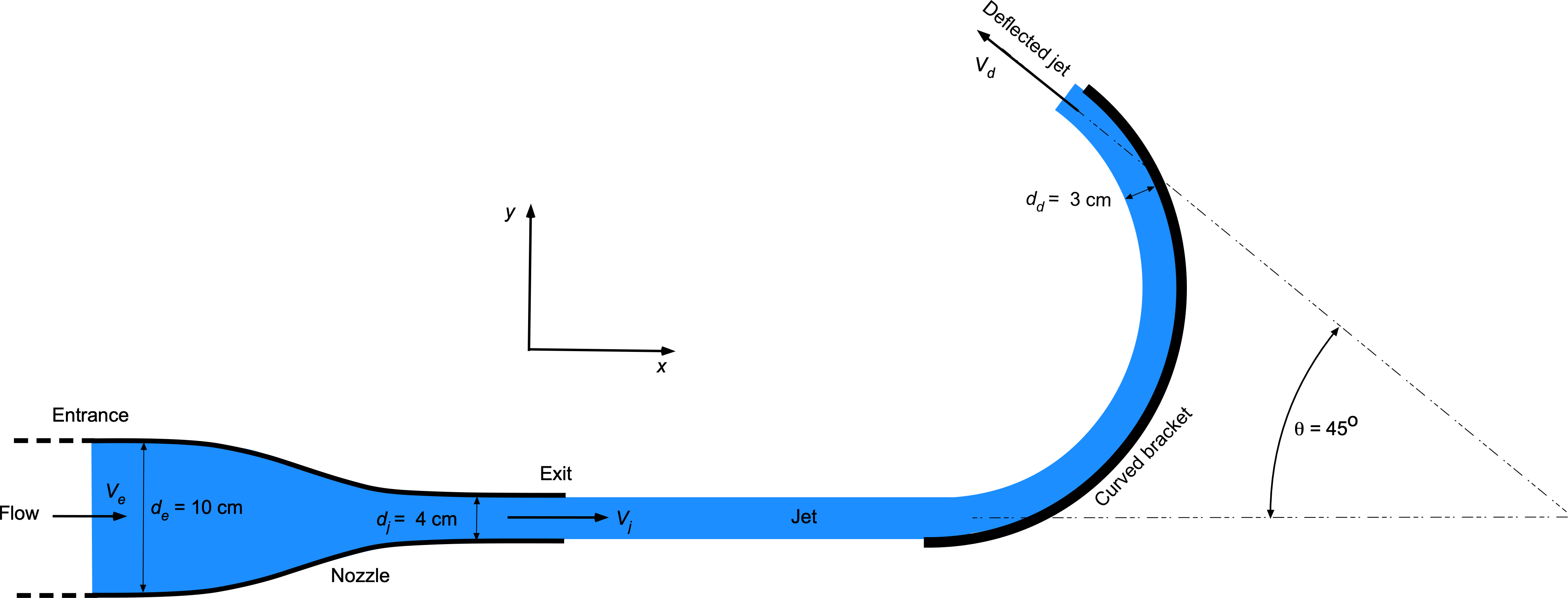
Draw an appropriate control surface with annotations to analyze the problem.
Calculate the velocity of the water entering and exiting the nozzle ( $V_e$ and $V_j$ ).
Calculate the change in pressure ( $\Delta p$ ) between the nozzle entrance and its exit.
Calculate the velocity ( $V_d$ ) of the water in the deflected jet.
Determine the magnitude and direction of the force on the bracket.

1. This is what the control surface with annotations should look like. Notice that there are two control volumes, with the output flow of one control volume feeding into the other one.

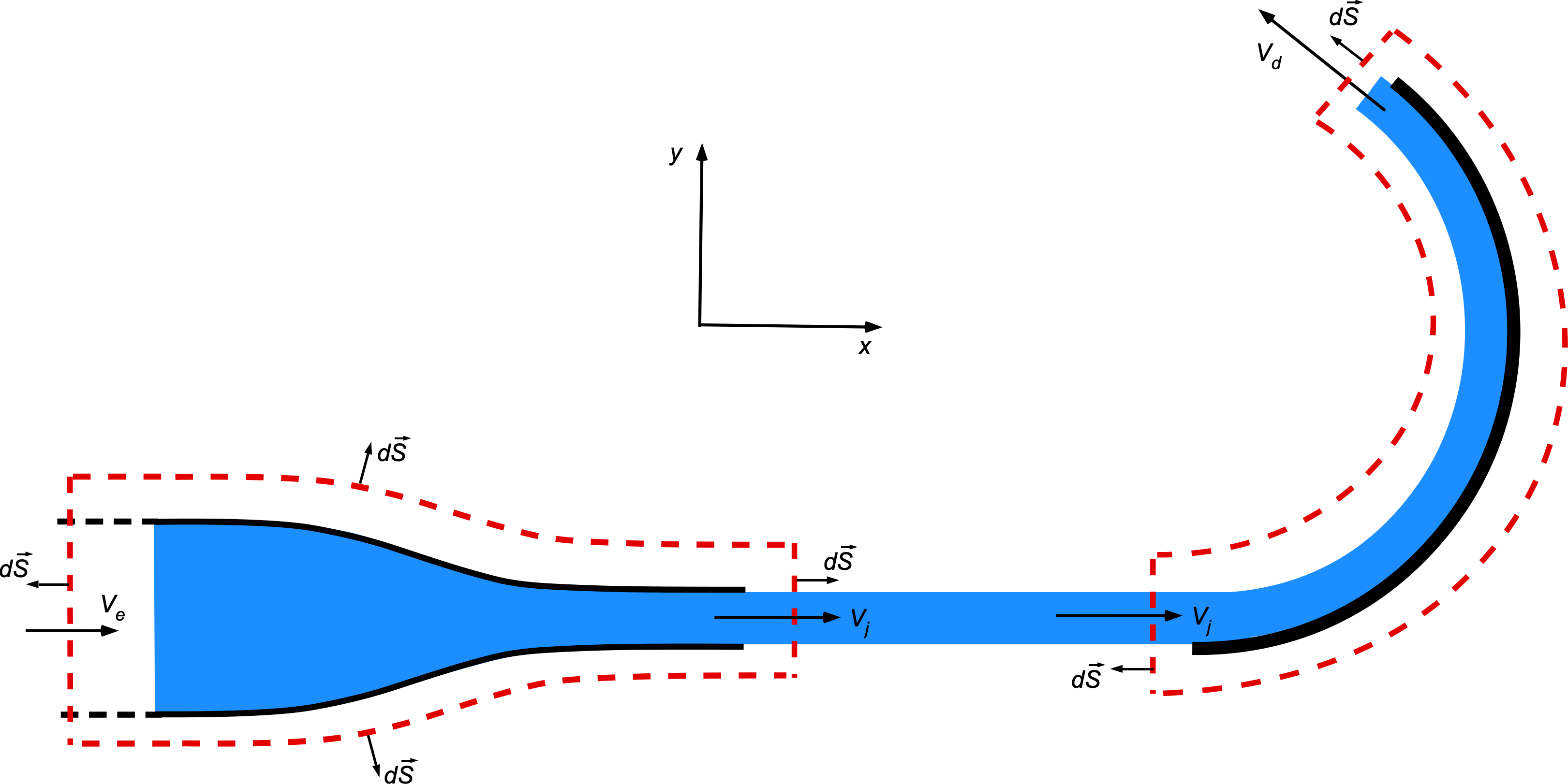
2. The velocity of the water entering and exiting the nozzle can be determined using the conservation of mass (continuity equation), i.e.,

$\dot{m} = \rho_w \, A_e \, V_e = \rho_w \, A_j \, V_j$

The entrance area ( $A_e$ ) is

$A_e = \frac{\pi d_e^2}{4} = \frac{\pi (10.0/100)^2}{4} = 0.00785 \, \text{m}^2$

Therefore, the entrance velocity is

$V_e = \frac{\dot{m}}{\rho_w \, A_e} = \frac{6.0}{1000 \times 0.00785} = 0.765 \, \text{m/s}$

For the exit velocity, $V_j$ , then using the continuity equation gives

$V_j = V_e \left( \frac{A_e}{A_j} \right) = 0.765 \left( \frac{\pi \, 10.0^2}{\pi \, 4.0^2} \right) = 4.78 \, \text{m/s}$

3. Using Bernoulli’s equation, then

$p + \frac{1}{2} \rho V^2 = \text{constant} \implies p_e + \frac{1}{2} \rho V_e^2 = p_j + \frac{1}{2} \rho V_j^2$

Rewriting for the pressure change gives

$p_e - p_j = \Delta p = \frac{1}{2} \rho \left( V_j^2 - V_e^2 \right)$

Substituting values then gives

$\Delta p = 0.5 \times 1000 \times \left(4.78^2 - 0.765^2 \right) = 11,350.5 \, \text{Pa}$

4. The velocity of the deflected jet can be determined using continuity, i.e.,

$\dot{m} = \rho_w \, A_j \, V_j = \rho_w \, A_d \, V_d$

Rearranging gives

$V_d = V_j \left( \frac{A_j}{A_d} \right) = 4.78 \left( \frac{\pi \, 4.0^2}{\pi \, 3.0^2} \right) = 8.43 \, \text{m/s}$

5. The force on the bracket is determined from the rate of change of momentum. Assuming the system is open to the atmosphere and pressure forces are insignificant, then

$F_x = -\dot{m} \, V_d \, \cos(45^\circ) - \dot{m} \, V_j$

Substituting the values gives

$F_x = -6.0 \times \left( 8.43 \times 0.707 + 4.78 \right) = -62.07 \, \text{N}$

For the ${y}$ -direction, then

$F_y = \dot{m} \, V_d \, \sin(45^\circ) = 6.0 \times 8.43 \times 0.707 = 35.72 \, \text{N}$

The reaction force on the bracket is then

$\vec{R} = -\vec{F} = (-F_x, -F_y) = (62.07, -35.72) \, \text{N}$

which is to the right and downward.

Worked Example #32

Water flows from a circular pipe through a nozzle and is diverted as a circular jet onto an inclined plate with a circular groove that maintains the jet’s circular form, as illustrated in the figure below. The diameters are $d_1 = 5$ cm, $d_2 = 3$ cm and $d_3 = 2.5$ cm. If the flow rate is $Q$ = 0.00687 m ${^{3}}$ s $^{-1}$ , what force is required to hold the plate in position? Assume uniform flow properties across any cross-section of the flow. Assume a steady flow with no losses. Neglect all pressure and gravitational effects. Hint: Be sure to show the control surface around the problem and the directions of the unit normals. The density of water is 1,000 kg m $^{-3}$ .

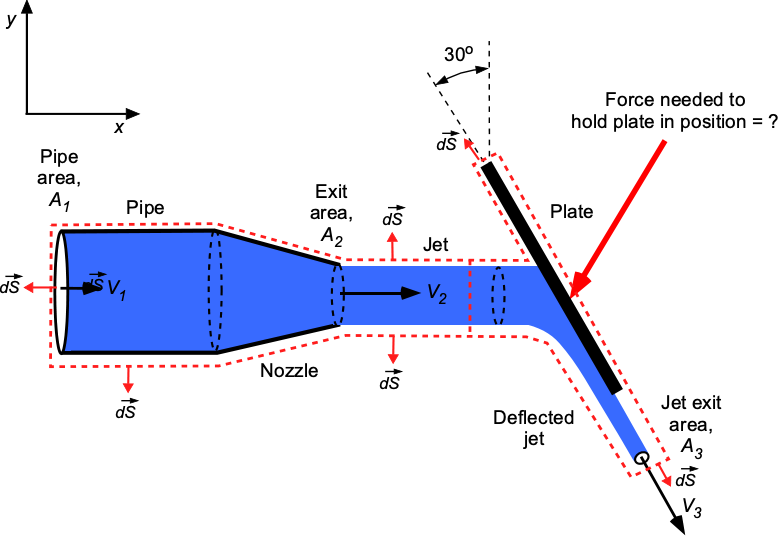
The relevant forms of the continuity and momentum equations based on the assumptions are

$\oiint_S \varrho \vec{V} \cdot d\vec{S} = 0$

and

$\vec{F} = \oiint_S (\varrho \vec{V} \cdot d\vec{S}) \vec{V}$

In one-dimensional form (uniform flow properties across any cross-section), the continuity equation can be written as

$\sum_{i = 1}^{N} \varrho_i \, V_i \, A_ i = 0$

For flow in the $x-y$ plane, the corresponding momentum equation in terms of its scalar components is

$F_x = \dot{m} \, \Delta u$

where $\Delta u$ is the change in the flow velocity in the ${x}$ direction, and

$F_y = \dot{m} \, \Delta v$

where $\Delta v$ is the change in the flow velocity in the ${y}$ direction, and where in each case $\dot{m}$ is the mass flow rate.

The control volume is shown in the figure below. From 1 to 2 over the nozzle, then

$-\varrho_1 \, V_1 \, A_1 + \varrho_2 \, V_2 \, A_2 = 0$

Because the flow is incompressible, then

$- V_1 \, A_1 + V_2 \, A_2 = 0$

so

$V_2 = \left( \frac{A_1}{A_2} \right) V_1 = \left( \frac{d_1}{d_2} \right)^2 V_1$

We are given the flow rate, $Q$ , so

$V_1 = \frac{Q}{A_1}$

where

$A_1 = \frac{\pi d_1^2}{4} = \frac{\pi (0.05)^2}{4} = 0.001963~\text{m}^2$

Inserting the values gives

$V_1 = \frac{0.00687}{0.001963} = 3.50~\text{m/s}$

The velocity at section 2 is

$V_2 = \left( \frac{d_1}{d_2} \right)^2 V_1 = \left( \frac{0.05}{0.03} \right)^2 \times 3.50 = 2.778 \times 3.50 = 9.72~\text{m/s}$

The mass flow rate is

$\dot{m} = \varrho Q = 1{,}000 \times 0.00687 = 6.87~\text{kg/s}$

From sections 2 to 3, the flow is deflected by a plate. Applying conservation of mass, then

$- V_2 A_2 + V_3 A_3 = 0 \quad \Rightarrow \quad V_3 = \left( \frac{A_2}{A_3} \right) V_2 = \left( \frac{d_2}{d_3} \right)^2 V_2$

$V_3 = \left( \frac{0.03}{0.025} \right)^2 \times 9.72 = 1.44 \times 9.72 = 14.0~\text{ m/s}$

The force on the fluid is equal to its time rate of change of momentum, i.e.,

$F_x = \dot{m} (V_3 \sin\theta - V_2) \quad \text{and} \quad F_y = \dot{m} ( 0 - V_3 \cos\theta) = - \dot{m} V_3 \cos\theta$

Substituting the values gives

$F_x = 6.87 (14.0 \times 0.5 - 9.72) = 6.87 (7.0 - 9.72) = 6.87 \times (-2.72) = -18.7~\text{ N}$

and

$F_y = -6.87 \times 14.0 \times 0.866 = -6.87 \times 12.12 = -83.3~\text{ N}$

Therefore, the force on the fluid is

$\vec{F} = -18.7 \, \vec{i} - 83.3 \, \vec{j}~\text{ N}$

and the force on the plate is

$\vec{R} = -\vec{F} = 18.7 \, \vec{i} + 83.3 \, \vec{j}~\text{ N}$

which is upward and to the right.

License

Icon for the Creative Commons Attribution-NonCommercial-NoDerivatives 4.0 International License

Introduction to Aerospace Flight Vehicles Copyright © 2022–2025 by J. Gordon Leishman is licensed under a Creative Commons Attribution-NonCommercial-NoDerivatives 4.0 International License, except where otherwise noted.

Digital Object Identifier (DOI)

https://doi.org/https://doi.org/10.15394/eaglepub.2022.1066.9

License

Digital Object Identifier (DOI)

Share This Book