Altitude Definitions & Measurement

J. Gordon Leishman

doi:https://doi.org/10.15394/eaglepub.2022.1066.n30

35 Altitude Definitions & Measurement

Introduction

As with its airspeed, measurements of the altitude of an aircraft are also critical to both its piloting and its engineering. Pilots are concerned about the altitude of an aircraft relative to sea level or above the ground, i.e., for takeoff and landing or terrain avoidance. Naturally, the altitude reference (datum) used is essential so that all aircraft fly at altitudes measured relative to the same standard reference, which is necessary for air traffic control and collision avoidance. Pilots also need to anticipate their aircraft’s performance, which primarily depends on altitude and outside air temperature.

Engineers, however, are more interested in obtaining a measurement of air density at a given flight altitude. In this case, altitude measurements can be related to air density by measuring pressure and temperature and then calculating density by invoking the equation of state. In addition, an altimeter is a pressure-measuring instrument by design, so it is possible to determine the corresponding local air pressure by measuring altitude. Outside air temperature can also be measured during flight using a thermometer. Therefore, the proper basis of altitude measurement and how such measurements are used in engineering practice to find air density must be understood.

Learning Objectives

Understand how an altimeter works and how to read one.
Appreciate the principles associated with altitude measurement.
Know the differences between pressure altitude and density altitude.
Be able to calculate density altitude from values of temperature and pressure altitude.

What is an Altimeter?

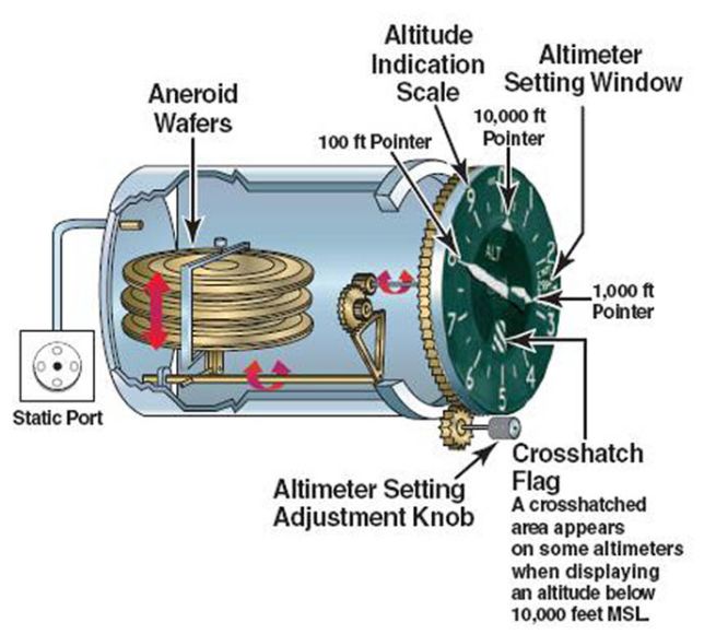
Like the airspeed indicator (ASI), an altimeter is a pressure-measuring (pneumatic) instrument. An altimeter responds to the local ambient static pressure, so the altimeter must be connected to the static pressure reference source on the aircraft, i.e., to the static port. However, unlike an airspeed indicator with two ports, one for total (or ram) pressure and the other for static pressure, an altimeter has only one port for static pressure. The mechanical design of an altimeter is shown in the schematic below. Although it looks relatively simple, it is a delicate and precise instrument and requires careful and repeated calibrations to be used in aviation practice.

The inner workings of an altimeter. The face of the altimeter has a circular scale like a clock with three-pointers to measure altitude to an accuracy of about $\pm$ 10 feet.

Inside the altimeter, the expansion and contraction of an evacuated aneroid wafer stack are detected by a system of levers and gears and then displayed by the rotational movement of the pointer (needles) on a face with a scale, much like that of a clock. The display of an altimeter has three needles or hands: One for 100s of feet, another for 1,000s of feet, and the third for 10,000s of feet. Notice from the figure above that the altimeter also has a setting window called the Kollsman window. On the bottom left side of the altimeter is a knurled adjustment knob used to adjust the reference pressure displayed in the Kollsman window. The altimeter, therefore, will read differently depending on the reference value of pressure set in this window.

Reading an Altimeter

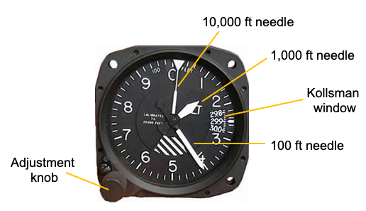
Reading an altimeter is relatively easy but does take some practice. In reference to the image below, the 10,000-foot pointer is the longest and narrowest needle on the altimeter; it rotates by one unit for every 10,000-foot change in altitude. The shortest and widest needle measures increments of 1,000 feet, so a full rotation of the needle is an altitude increment of 10,000 feet. The medium-length hand reads 100s of feet so that a full rotation would be an altitude increment of 1,000 feet. In this regard, the numbers on the dial each represent 100-foot increments, and the tick marks between the numbers represent increments of 20 feet. For example, in the case shown below, the 100-foot pointer is just past the number 4 (i.e., 410 feet), the 10,000-foot pointer has just moved from 0, and the 1,000-foot pointer is between the 1 and the 2, so 1,000 feet plus. Therefore, in this case, the altimeter, as shown, reads 1,410 feet relative to the pressure datum value set in the Kollsman window.

In this case, the face of the altimeter shows a reading of 1,410 ft.

All aviation altimeters are formally calibrated according to the pressure variations in the ISA. Typically, the mechanical design of an altimeter means that it can only be calibrated within a certain tolerance, $\pm$ 20 feet being typical for a GA aircraft, which is sufficient for piloting use. However, for engineering use, a more precise and formal calibration will be needed so that mechanical errors can be accounted for, just as in the case of the ASI. This calibration is obtained by calibrating the altimeter in a vacuum tank relative to known pressure values or against a reference altimeter that has been previously calibrated. Again, the results for the mechanical correction are usually provided as a chart or a table of values along with those for the airspeed indicator.

Test Your Understanding of How to Read an Altimeter

Please look at the faces of the three altimeters, A, B, and C, as shown below. What is the altitude reading in each case?

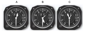
Answers: A: 10,500 feet. B: 14,500 feet. C: 9,500 feet

Review of ISA Pressure & Density Variations

Before proceeding with the formal definitions of pressure altitude and density altitude, it is helpful to summarize the previously derived equations of the International Standard Atmosphere or ISA.

ISA Temperature Variations

The temperature $T$ in the international standard atmosphere is given by

(1) $\begin{equation*} T = T_0 - B \, h = 59.0 -\left( \frac{3.57}{1,000} \right) h \quad \hbox{in units of $^{\circ}$F} \end{equation*}$

or

(2) $\begin{equation*} T = 59.0 - 0.00357 h \quad \hbox{in units of $^{\circ}$F} \end{equation*}$

where $h$ , in this case, is expressed in feet (ft), and $B$ is called the standard atmospheric lapse rate. This temperature lapse equation is valid only up to the troposphere’s limits or about 36,000 ft. The value of $B$ is 3.57 $^{\circ}$ F per 1,000 ft of altitude or 0.00357 $^{\circ}$ F per ft = 0.00357 $^{\circ}$ R per ft.

In SI units, the ISA temperature lapse equation can be written as

(3) $\begin{equation*} T = T_0 - B h = 15.0 - \left( \frac{6.5}{1,000} \right) h\quad \hbox{in units of $^{\circ}$C} \end{equation*}$

or

(4) $\begin{equation*} T = 15 - 0.0065 h\quad \hbox{in units of $^{\circ}$C} \end{equation*}$

where $h$ is expressed in meters (m), and the ISA lapse rate, in this case, is 6.5 $^{\circ}$ C per 1,000 m. This lapse rate is also equivalent to 1.981 $^{\circ}$ C per 1,000 ft, giving

(5) $\begin{equation*} T = 15 - 0.001981 \, h \quad \hbox{in units of $^{\circ}$C} \end{equation*}$

with $h$ being measured in feet (ft). Measuring altitude in feet for aeronautical and aviation purposes is standard practice.

Often, the ratio of the ISA temperature at a given altitude to the MSL temperature is used, which is given the symbol $\theta$ , i.e.,

(6) $\begin{equation*} \theta = \frac{T}{T_0} \end{equation*}$

ISA Pressure Variations

The resulting local pressure in the ISA, $p$ , at any altitude $h$ relative to the value at MSL, $p_0$ , is

(7) $\begin{equation*} \frac{p}{p_0} = \delta = \left( 1 - \frac{B}{T_0} \, h \right)^{g/RB} = \left( 1 - 6.883\times 10^{-6} \, h \right)^{5.256} \end{equation*}$

where $h$ in this latter equation is measured in feet (ft). Notice that in USC units, then

(8) $\begin{equation*} \frac{B}{T_0} = \frac{3.57/1,000}{59.0+ 459.67} = 6.883\times 10^{-6} \end{equation*}$

The gas constant for air, $R$ , in USC units is 1716.49 ft lb slug $^{-1}$ R $^{-1}$ and in SI units it is 287.057 J kg $^{-1}$ K $^{-1}$ . Therefore, the value of $g/RB$ , which is a non-dimensional grouping, is

(9) $\begin{equation*} \frac{g}{R B} = \frac{32.17}{1716.49 \times 0.00357} = \frac{9.81}{287.057 \times 0.0065} = 5.256 \end{equation*}$

so its numerical value does not depend on the unit system. If $h$ were to be measured in meters (m), then

(10) $\begin{equation*} \frac{p}{p_0} = \delta = \left( 1 - \frac{B}{T_0} \, h \right)^{5.256}= \left( 1 - 2.256\times 10^{-5} \, h \right)^{5.256} \end{equation*}$

where in this case, using SI units gives

(11) $\begin{equation*} \frac{B}{T_0} = \frac{6.5/1,000}{15.0+ 273.15} = 2.256\times 10^{-5} \end{equation*}$

Remember that under standard MSL conditions, the value of $p_0$ is 2116.4 lb/ft $^2$ or 101.325 kN/m $^{^2}$ .

ISA Density Variations

In accordance with the assumptions made with the ISA model, the pressure and density can be related using the equation of state, i.e.,

(12) $\begin{equation*} \frac{\varrho}{\varrho_0} = \frac{p}{p_0} \left( \frac{T_0}{T} \right) \end{equation*}$

Therefore, if the local temperature corresponds to the standard local temperature in the ISA, i.e., $T_0 - B \, h$ , then

(13) $\begin{equation*} \frac{\varrho}{\varrho_0} = \frac{p}{p_0} \left( \frac{T_0}{T_0 - B \, h} \right) \end{equation*}$

and so the local density in the ISA relative to MSL is

(14) $\begin{equation*} \frac{\varrho}{\varrho_0} = \sigma = \bigg( 1 - \frac{B}{T_0} \, h \bigg)^{\left(\displaystyle{\frac{g}{R B} - 1 }\right)} = \left( 1 - 6.883\times 10^{-6} \, h \right)^{4.256} \end{equation*}$

where $h$ is measured in feet (ft). If $h$ is measured in meters (m), then

(15) $\begin{equation*} \frac{\varrho}{\varrho_0} = \sigma = \left( 1 - \frac{B}{T_0} \, h \right)^{4.256} = \left( 1 - 2.256\times 10^{-5} \, h \right)^{4.256} \end{equation*}$

Remember that under standard MSL conditions, the value of $\varrho_0$ is 0.002378 slugs/ft $^2$ or 1.225 kg/m $^{^3}$ .

Pressure Altitude

As previously described, an altimeter is a calibrated pressure gauge, its basis of calibration being the ISA. Therefore, it makes sense to use the altimeter to measure the air pressure the aircraft is flying, which is performed by determining the pressure altitude. By definition, the pressure altitude, $h_p$ , is the altitude in the ISA corresponding to the prevailing ambient local static pressure. The advantage of using pressure altitude as a reference is that its value is a function of the local ambient pressure alone.

Using the relationship for pressure in the ISA given by Eq. 10, the value of the pressure altitude, $h_p$ , as measured in feet (ft), is given by

(16) $\begin{equation*} h_p = \frac{T_0}{B} \left[ 1 - \left( \frac{p}{p_0} \right)^{0.1903} \right] = \frac{518.67}{0.00357} \left[ 1 - \left( \frac{p}{p_0} \right)^{0.1903} \right] \end{equation*}$

where $T_0 = 59.0 + 459.67 = 518.67^{\circ}$ R in USC, so

(17) $\begin{equation*} h_p = 145286.0 \left[ 1 - \left( \frac{p}{p_0} \right)^{0.1903} \right] \end{equation*}$

Remember that the unit of feet (ft) is used universally in aviation, and most altimeters are calibrated in feet. If required, the altimeter reading can be converted from feet to meters (m) by multiplying by 0.3048.

The measurement pressure altitude using the altimeter will also be subject to static position (SPE) errors and mechanical errors (instrument error correction or IEC), both of which need to be obtained from calibrations. The SPE error is obtained similarly to the airspeed indicator (ASI), where the true static pressure is measured well behind the aircraft during flight testing using a trailing cone apparatus. The SPE error, $\Delta h_{p_{\rm \, SPE}}$ , as it affects the true pressure altitude value, must be mapped out over the entire operating envelope of the aircraft. Likewise, with the IEC, the altimeter must be calibrated against a reference altimeter in an evacuated chamber to get $\Delta h_{p_{\rm \, IEC}}$ , an example being shown below.

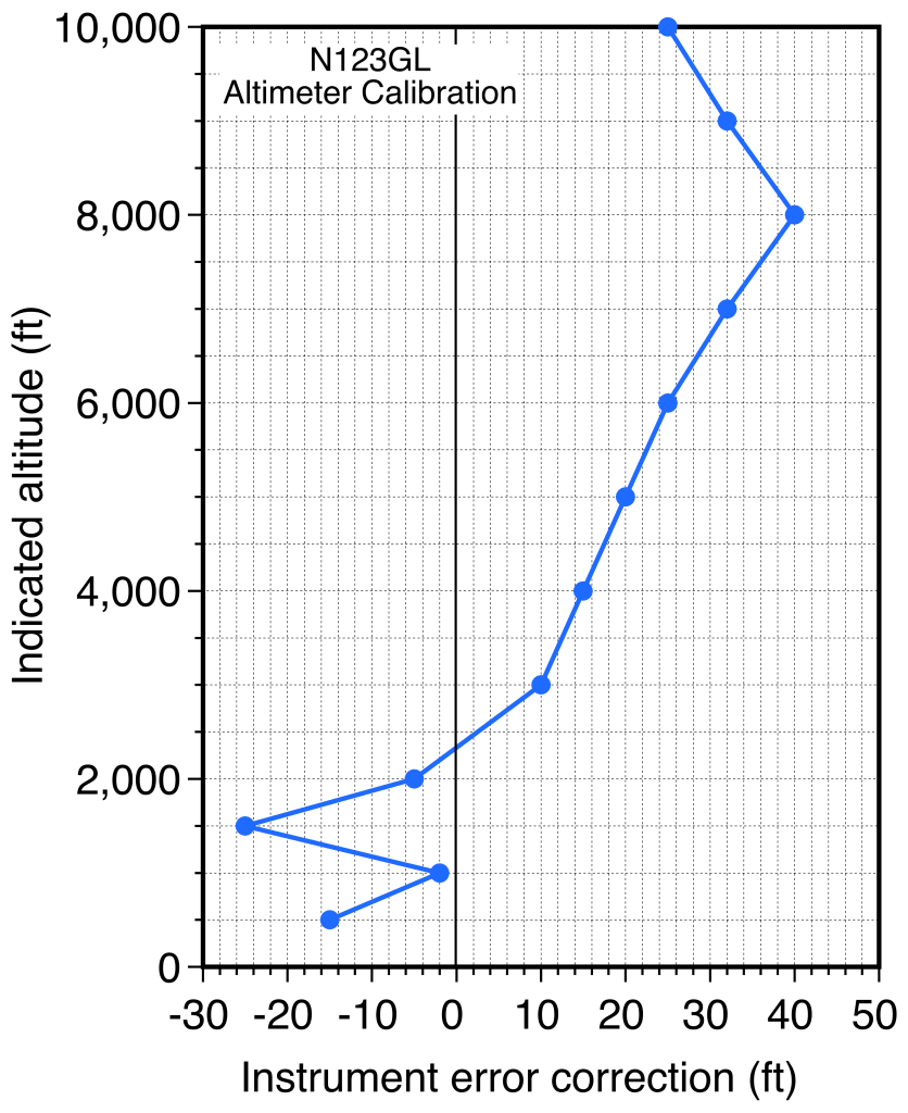
An instrument error calibration (IEC) chart for an altimeter shows that the altimeter may read high or low, depending on the specific altimeter. Each altimeter has its own IEC chart.

The corrected pressure altitude is then

(18) $\begin{equation*} h_p = h_{p_{\rm \, IND}} - \Delta h_{p_{\rm \, SPE}} - \Delta h_{p_{\rm \, IEC}} \end{equation*}$

where $h_{p_{\rm \, IND}}$ is the indicated pressure altitude on the altimeter. Such errors are usually small enough to be ignored for piloting purposes but must be accounted for in engineering calculations, including for aircraft and engine performance measurements.

Density Altitude

While pressure altitude can be measured directly on a suitably calibrated altimeter, ultimately, the density of the air in which it is flying affects the aircraft’s performance and its engines. To this end, a determination of the density of the air in which the aircraft is flying is required for engineering analysis and all types of performance work.

By definition, the density altitude, $h_{\varrho}$ , is the altitude in the ISA that corresponds to the prevailing ambient density. The value of the density altitude (again, measured in units of feet) can be obtained by rearranging Eq. 14 to get

(19) $\begin{equation*} h_{\varrho} = \frac{T_0}{B} \left[ 1 - \left( \frac{\varrho}{\varrho_0}\right)^{0.235}\right] = \frac{518.67}{0.00357} \left[ 1 - \left( \frac{\varrho}{\varrho_0}\right)^{0.235} \right] \end{equation*}$

Therefore,

(20) $\begin{equation*} h_{\varrho} = 145286.0 \left[ 1 - \left( \frac{\varrho}{\varrho_0}\right)^{0.235}\right] \end{equation*}$

where $h_{\varrho}$ is in units of feet.

Relating Density Altitude & Pressure Altitude

As previously explained, pressure altitude can be read directly using an altimeter, calibrated according to the ISA using Eq. 17. However, the reference value of pressure on the altimeter must be set to the standard MSL value. This is done by setting the reading Kollsman window to the MSL ISA value of 29.92 in Hg (inches of mercury) or 1013.2 millibars (depending on the specific altimeter), which are equivalent to the ISA MSL or $p_0$ values of 2116.4 lb/ft $^2$ or 101.325 kPa, respectively, in engineering units. The value of $h_p$ can then be directly read off the altimeter, assuming it is properly calibrated and that mechanical and static position errors are corrected.

Unlike pressure altitude, density altitude must be calculated from measurements of pressure altitude corrected for non-standard ambient temperature conditions relative to the ISA temperature standard. In this regard, “nonstandard” means that the local temperature deviates (i.e., higher or lower) from the ISA standard temperature value at any given pressure altitude. For example, the density will be lower for a temperature higher than the ISA standard temperature, but the density altitude will be higher than the pressure altitude.

Density Altitude Calculation

Recall that pressure and density are related using the equation of state, so the density ratio in the ISA can be written as

(21) $\begin{equation*} \frac{\varrho}{\varrho_0} = \frac{p}{p_0} \left( \frac{T_0}{T_{\rm {\tiny ISA}}} \right) \end{equation*}$

where $T_{\rm {\tiny ISA}}$ is the local standard temperature according to the ISA as given by

(22) $\begin{equation*} T_{\rm {\tiny ISA}} = T_0 - B h_p \end{equation*}$

where $h_p$ is the pressure altitude. If the pressure altitude and the outside air temperature, $T_{\rm {\tiny OAT}}$ , are both available (e.g., measured), then by using Eqs. 17 and 20 and some algebra, then the corresponding density altitude can be determined from

(23) $\begin{equation*} h_{\varrho} = \frac{T_0}{B} - \frac{T_{\rm {\tiny OAT}}}{B} \left( \frac{T_0 - B h_p}{T_{\rm {\tiny OAT}}} \right)^{\displaystyle{\frac{1}{1 - RB/g}}} \end{equation*}$

Because $g/RB = 5.256$ then

(24) $\begin{equation*} h_{\varrho} = \frac{T_0}{B} - \frac{T_{\rm {\tiny OAT}}}{B} \left( \frac{T_0 - B h_p}{T_{\rm {\tiny OAT}}} \right)^{1.235} \end{equation*}$

This means that Eq. 24 can be used to find the density altitude for any given pressure altitude and outside air temperature values. It can also be seen that if the local temperature equals the standard ISA temperature at the pressure altitude, i.e., $T_{\rm {\tiny OAT}} = T_0 - B h_p = T_{\rm {\tiny ISA}}$ , then $h_{\varrho} = h_p$ . Remember that all temperature values in these equations are absolute temperatures.

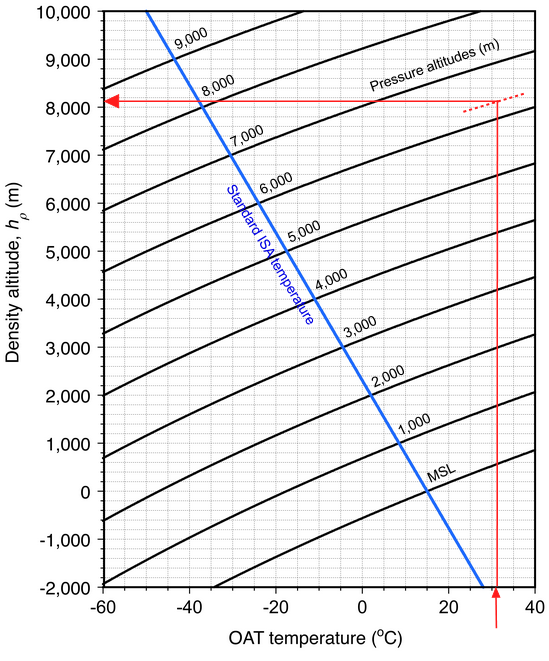
Armed with these equations, it is now possible to examine the variations in density altitude with temperature changes for different pressure altitude values, as shown in the chart below in SI units. In this regard, it should be remembered that the value of $B$ in SI units $B$ is 6.5 $^{\circ}$ C per 1,000 m or 1.981 $^{\circ}$ C per 1,000 ft. The diagonal lines are values of constant pressure altitude. The blue line is the standard ISA temperature variation, giving $h_{\varrho} = h_p$ . Taking as an example $T_{\rm {\tiny OAT}} = 32^{\circ}$ C and $h_p = 6,300$ m, then by following the red lines on the chart, the chart gives an estimated value of $h_{\varrho}$ of 8,200 m.

A pressure/density altitude chart in SI units from which density altitude can be estimated from measurements of pressure altitude and outside air temperature.

The same type of presentation showing the variation in density altitude with temperature changes for different pressure altitude values is shown in the chart below in USC units. In this case, $B$ is 3.57 $^{\circ}$ F per 1,000 ft of altitude or 0.00357 $^{\circ}$ F per ft = 0.00357 $^{\circ}$ R per ft. Again, taking as an example where $T_{\rm {\tiny OAT}} = 85^{\circ}$ F and $h_p = 17,500$ ft, then following the red lines on the chart gives an estimated value of $h_{\varrho}$ of 23,000 ft.

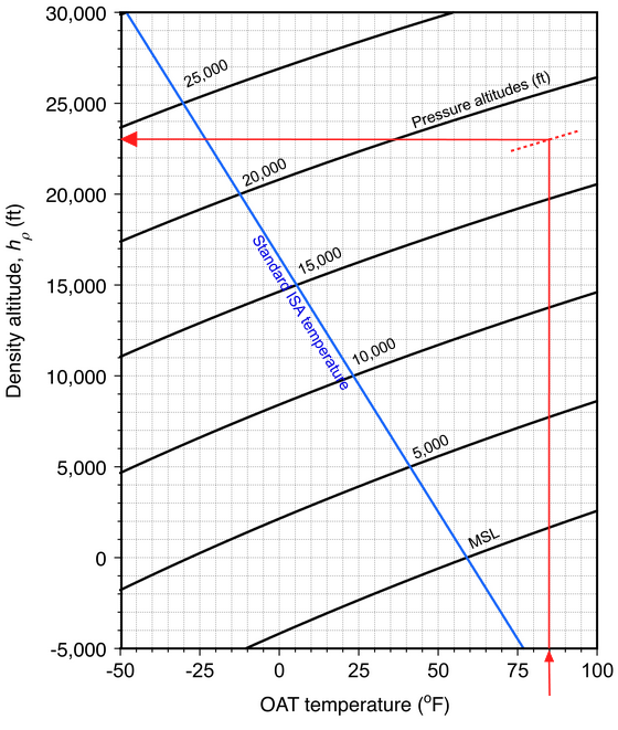
A pressure/density altitude chart in USC units from which density altitude can be estimated from measurements of pressure altitude and outside air temperature.

Notice that interpolation is inevitably required when using these charts, but the eye and brain are excellent interpolators. Nevertheless, while the charts are a reasonable visual interpretation of the differences between pressure altitude and density altitude for variations in non-standard temperature, they should not be used for engineering purposes instead of the ISA equations.

Density Ratio Calculation

Another useful metric to be able to calculate from the pressure altitude and outside air temperature is the density ratio, $\sigma$ , which is often required to be known for aircraft and engine performance analysis. The value of $\sigma$ can be obtained from

(25) $\begin{eqnarray*} \sigma = \frac{\varrho}{\varrho_0} & = &\frac{T_0}{(T_{\rm {\tiny OAT}} +273.16)} \left( 1 - \frac{B h_p}{T_0} \right)^{5.252} \nonumber \\ & = & \frac{288.16}{(T_{\rm {\tiny OAT}} +273.16)} \left( 1 - \frac{0.001981~h_p}{288.16} \right)^{5.252} \end{eqnarray*}$

where the local pressure altitude, $h_p$ , is in feet and the local $T_{\rm {\tiny OAT}}$ is in units of $^{\circ}$ C or using

(26) $\begin{equation*} \sigma = \frac{\varrho}{\varrho_0} = \frac{518.4}{(T_{\rm {\tiny OAT}} +4 59.4)} \left( 1 - \frac{0.001981 \, h_p}{288.16} \right)^{5.252} \end{equation*}$

where $h_p$ is in feet and $T_{\rm {\tiny OAT}}$ is in units of $^{\circ}$ F.

It is also useful to remember that the equation of state can be written as

(27) $\begin{equation*} \delta = \sigma \, \theta \end{equation*}$

which is useful when converting back and forth between density, pressure, and temperature in the ISA.

Worked Example #1 – Calculating the density altitude

Use the ISA equations to calculate the corresponding density altitude, given a measured outside air temperature of 32 $^{\circ}$ C and a pressure altitude of 6,300 m.

The relevant ISA equation is

$h_{\varrho} = \frac{T_0}{B} - \frac{T_{\rm {\tiny OAT}}}{B} \left( \frac{T_0 - B h_p}{T_{\rm {\tiny OAT}}} \right)^{1.235}$

where in this case $T_{\rm {\tiny OAT}}$ = 32 $^{\circ}$ C and $h_p$ = 6,300 m. Inserting the other SI values gives

$h_{\varrho} = \frac{288.15}{0.0065} - \frac{T_{\rm {\tiny OAT}}}{0.0065} \left( \frac{288.15 - 0.0065 \times 6,300}{32.0 + 273.15} \right)^{1.235} = 8,136~\mbox{m}$

This result means that even though the altimeter will read 6,300 m, the aircraft will behave from a performance perspective as if flying at an altitude of 8,136 m because of the higher than standard air temperature. Notice also that this calculated value of density altitude agrees with the chart example given previously.

Measuring Outside Air Temperature

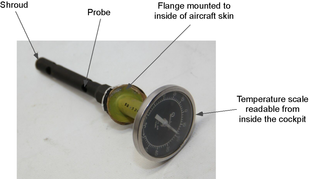
In aviation terminology, the outside air temperature (OAT) refers to the air surrounding an aircraft during its flight. However, its value is assumed to be unaffected by the passage of the aircraft through it, i.e., it is often referred to as a static temperature. A measurement of the outside air temperature (OAT) is required to determine the air density for engineering purposes. A simple OAT gauge can be used below a Mach number of 0.3 (the incompressible flow regime), as shown in the photograph below, which provides a relatively accurate measurement of the static air temperature. In this application, the probe is shrouded from the airflow, which minimizes temperature errors from any heating caused by direct sunlight. The probe typically protrudes through the aircraft’s windshield or the side of the fuselage at the cockpit to expose the probe to the atmospheric air. The instrument head is mounted inside the windshield in a suitable location where the pilot can easily read it.

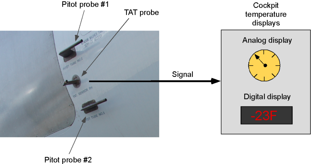
A temperature probe can be suitably mounted through a window or the fuselage skin to read the outside air temperature (OAT).

At higher airspeeds, the compressibility of the flow makes accurate air temperature measurements somewhat more challenging. In this case, the total air temperature (TAT) is measured, which is the static air temperature plus any temperature rise caused by the effects of the airflow, i.e., a total temperature. TAT probes are constructed to measure this temperature value accurately and transmit the signals for cockpit indication as airspeed and Mach number and for use in various engine and aircraft systems, as shown in the figure below.

Outside air temperature (OAT) or total temperature (TAT) probes are needed to measure the local ambient air temperature, which can be displayed on various cockpit instruments.

The design of a TAT probe is complicated by the possibility of ice forming on it, just as it might do on a total pressure or Pitot probe. Therefore, the TAT probe must be heated. In this regard, the ambient airflow must be directed carefully through the probe to measure the actual outside air temperature without any effects from the heater. Several manufacturers specialize in TAT probes for aircraft applications.

Practical Use of Density Altitude

The ISA equations are used universally for aircraft performance standardization and flight test evaluations. In many cases, a rapid estimation of the density altitude can be helpful for piloting purposes. For example, the information in an aircraft’s operating manual may be expressed as a function of density altitude. As previously discussed, pressure altitude can be measured directly on the altimeter. In contrast, density altitude is determined by calculating the pressure altitude and local outside air temperature at the same altitude.

Linearization of the ISA Equations

It will be seen from the graphs of density altitude changes versus temperature for a given pressure altitude that the relationship is almost linear, which suggests an approximation to Eq. 24 is likely to be useful for rapid estimates of density altitude, i.e., for piloting purposes when a quick estimate is required such as for advance flight planning. Such linearizations, however, would never be used for flight test work.

To linearize Eq. 24, it can be expanded as a Taylor series about the ISA standard temperature value at a given pressure altitude and retaining only the first derivative of the series to give

(28) $\begin{equation*} h_{\varrho} \approx h_p + \frac{R}{g - R B} \left( T_{\rm {\tiny OAT}} - T_{\rm {\tiny ISA}} \right) \end{equation*}$

where $T_{\rm {\tiny ISA}}$ is the ISA standard temperature at the given $h_p$ , i.e.,

(29) $\begin{equation*} T_{\rm {\tiny ISA}} = T_0 - B h_p \end{equation*}$

in appropriate units. Notice that

(30) $\begin{equation*} \frac{R}{g - R B} = \frac{287.057}{9.81 - 287.057 \times 0.0065} = 36.135~\mbox{m/$^{\circ}$C} \end{equation*}$

Therefore,

(31) $\begin{equation*} h_{\varrho} \approx h_p + 36.13 \left( T_{\rm {\tiny OAT}} - T_{\rm {\tiny ISA}} \right) \end{equation*}$

when $h_{\varrho}$ and $h_p$ are in units of meters and $T_{\rm {\tiny OAT}}$ and $T_{\rm {\tiny ISA}}$ are in units of $^{\circ}$ C. Remember that $T_{\rm {\tiny ISA}}$ in this equation is the ISA standard temperature at the given value of $h_p$ . Alternatively, in mixed units, then

(32) $\begin{equation*} h_{\varrho} \approx h_p + 118.55 \left( T_{\rm {\tiny OAT}} - T_{\rm {\tiny ISA}} \right) \end{equation*}$

where $h_{\varrho}$ and $h_p$ are in units of feet and $T_{\rm {\tiny OAT}}$ and $T_{\rm {\tiny ISA}}$ are in $^{\circ}$ C. Finally, in entirely USC units, then

(33) $\begin{equation*} \frac{R}{g - R B} =\frac{1716.49}{32.17 - 1716.49 \times 0.00357} = 65.91~\mbox{ft/$^{\circ}$F} \end{equation*}$

so the density altitude will be

(34) $\begin{equation*} h_{\varrho} \approx h_p + 65.91 \left( T_{\rm {\tiny OAT}} - T_{\rm {\tiny ISA}} \right) \end{equation*}$

where $h_{\varrho}$ and $h_p$ are in feet and $T_{\rm {\tiny OAT}}$ and $T_{\rm {\tiny ISA}}$ are in $^{\circ}$ F.

Therefore, the linearization of the ISA equations shows that density altitude exceeds pressure altitude by about 120 ft per ^oC or 65 ft per ^oF that the temperature exceeds the standard ISA temperature value at a given pressure altitude. However, these results are approximate but reasonably accurate for moderate variations of non-standard ISA temperature at a given pressure altitude. However, the approximations should never be used for engineering work instead of the ISA equations, i.e., Eqs. 17, 20 and 24.

Worked Example #2 – Calculating the approximate density altitude

Given a measured outside air temperature of 32 $^{\circ}$ C and a pressure altitude of 6,300 m, calculate the corresponding density altitude using the approximate conversion rules.

The relevant ISA equation in Worked Example #1 gives $h_{\varrho}$ = 8,136 m. The approximation for density altitude from Eq. 32 is

$h_{\varrho} \approx h_p + 36.13 \left( T_{\rm {\tiny OAT}} - T_{\rm {\tiny ISA}} \right)$

The standard ISA temperature at 8,136 m is

$T_{\rm {\tiny ISA}} = T_0 - B h_p = 15 - 0.0065 \times 6,300 = -15.95~\mbox{$^{\circ}$C}$

Therefore, inserting the numerical values gives

$h_{\varrho} \approx 6,300 + 36.13 \left( 32.0 - (-15.95) \right) = 6,300 + 1,732 = 8,032~\mbox{m}$

Therefore, this density altitude value underpredicts the value given by the complete ISA equation by only about 100 m.

Reference Pressures for Piloting

To adjust the altimeter for variations in atmospheric pressure, the setting in the Kollsman window must be continuously adjusted by the pilot of an aircraft. In the U.S., the altimeter reference pressure is generally set to the local mean sea level (MSL) pressure so that all aircraft in the same vicinity will fly with respect to the local MSL reference. In this case, when the aircraft is on the ground, the altimeter should read the approximate field elevation, which is also a way to check if the altimeter is working as it should. The local value of MSL pressure at any time is available from air traffic control, weather stations, etc.

In other countries, altimeter settings called QFE and QNH are used. The QFE is the reference pressure set in the Kollsman window of the altimeter to indicate its height above the reference elevation being used, which is usually the elevation of an airfield. In this case, the altimeter will read zero when the aircraft is on the ground. The QNH is the reference pressure that indicates the height above sea level on the altimeter, which is the default in the U.S.

Above 18,000 ft, pilots are required to set the altimeter to the standard MSL reference pressure of 29.92 inches of Hg, in which case the altitude reading is referred to as a flight level. Therefore, flight level 230 is equivalent to a pressure altitude of 23,000 ft. All aircraft must be flown at higher altitudes relative to the same pressure datum. Over the Atlantic Ocean, for example, horizontal separation distances between aircraft may only be a few miles and vertical separation altitudes as little as 1,000 feet, so all aircraft must fly at an altitude measured with respect to the same pressure datum.

Worked Example #3 – For pilots & engineers

Suppose the reported local altimeter setting at your local Florida airport before an approaching hurricane is 29.32 inches of Hg, which is the pressure at sea level for that airport and the time of day. The airport is 88 ft above MSL and only has a 2,000 ft long runway. Moving your Cessna 172 airplane and family to Alabama would be best to avoid the hurricane. The reported local temperature at their airport is 34^oC, with light showers. What is the estimated density altitude for takeoff, and should you worry?

The difference between the reported altimeter setting and the standard ISA reference is

$29.32 - 29.92 = -0.6~\mbox{inches of Hg}$

The negative value means the local pressure is lower than the standard pressure, so even the density altitude at ISA standard temperature will be higher. Converting to units of feet gives the equivalent pressure altitude for an altimeter setting of 29.32 as

$h_p = 924.664 \times 0.6 = 555~\mbox{ft}$

where the value of 924.664 is the conversion factor from inches of Hg to feet. The standard ISA temperature at 555 ft is

$T_{\rm {\tiny ISA}} = T_0 - B h_p = 15.0 - 0.0065 \times 555.0 = 11.4~\mbox{$^{\circ}$C}$

Using the approximation in Eq. 32 to obtain density altitude from pressure altitude gives

$h_{\varrho} \approx h_p + 118.55 \left( T_{\rm {\tiny OAT}} - T_{\rm {\tiny ISA}} \right)$

with heights being measured in feet and temperatures in ^oC. Inserting the values gives

$h_{\varrho} \approx 555.0 + 118.55 \left( 34.0 - 11.4 \right) = 555.0 + 2,679.2 = 3,234~\mbox{ft}$

While the airport is 88 feet above MSL, the atmospheric conditions are such that the airplane will perform as if it were flying at an altitude of 3,200 feet. With a full passenger load, a short and wet runway, and a relatively modest powered Cessna 172, then yes, you should worry about getting off the runway in these conditions.

Electronic Flight Displays (EFD)

Advances in electronics and software engineering have significantly transformed the instrumentation used for modern aircraft with the introduction of Electronic Flight Displays (EFDs), often referred to as “glass cockpits.” Glass cockpits replace traditional analog gauges and instruments with digital displays, providing pilots with a more intuitive and information-rich interface, an example being shown in the figure below.

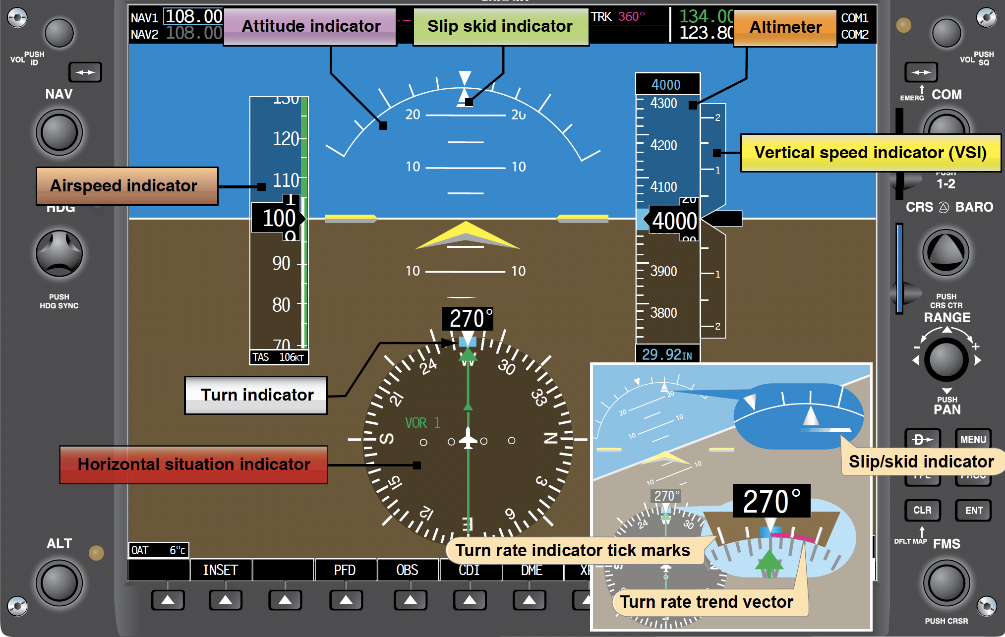
This is an example of an EFIS primary flight display that has largely replaced the traditional mechanical altimeter, airspeed indicator, and other analog instruments on modern aircraft.

EFDs utilize the same type of instrument inputs as traditional analog gauges; however, the processing system is entirely different. The Pitot static inputs are first received by an Air Data Computer (ADC.) The ADC computes the difference between the total and static pressure and uses equations to generate the information necessary to display the airspeed on the PFD. Outside air temperatures are also monitored and introduced into various components within the software and displayed on the PFD screen. These are the essential elements of an EFIS:

Pitot-Static Inputs: EFDs still receive pitot-static inputs where the pitot tube measures the total pressure, and the static ports measure the static pressure. As with a traditional mechanical instrument, the static pressure allows an altitude calculation, and the dynamic pressure provides the information necessary to calculate airspeed.
Analog-to-Digital Converter (ADC): The pitot-static inputs are received by an Analog-to-Digital Converter (ADC). The ADC converts the analog signals from the pitot-static system into a digital format that can be processed by the EFD’s software and electronic system.
Air Data Computer (ADC): The ADC, a component within the EFD system, receives the digitized pitot-static inputs from the ADC. It computes the difference between total and static pressure to determine the airspeed. All necessary corrections for SPE can be included in the software. The ADC then generates the information required to display the airspeed on the Primary Flight Display (PFD) screen.
Outside Air Temperature (OAT) Monitoring: EFDs also monitor the outside air temperature. This temperature data is essential for various components within the aircraft systems, such as engine performance calculations and fuel management. The OAT and TAT are displayed on the PFD screen, providing pilots with real-time temperature information.

Summary & Closure

A measurement of the altitude of an aircraft during flight is fundamental to both its piloting and engineering. However, like the airspeed, the exact type of altitude must be carefully qualified. The density altitude affects aircraft and powerplant performance, which is a measure of the density of the air in which the aircraft is flying. Density altitude, however, cannot be measured directly and must be calculated based on pressure altitude and air temperature measurements. The higher the temperature above the standard temperature at a given altitude, the higher the density altitude, i.e., the lower the value of air density. The local density of the air will always affect both aircraft and powerplant performance.

5-Question Self-Assessment Quickquiz

For Further Thought or Discussion

An airplane is flying at a pressure altitude of 10,000 ft where the outside air temperature is -10^oF. What is the corresponding density altitude?
An ERAU aircraft is preparing to take off from Daytona Beach (identifier KDAB) in the summer, where the outside air temperature is 95^oF. What is the approximate density altitude, and why must the pilot know this?
If a pilot wants to estimate the approximate value of density altitude before takeoff, explain how that should be done using the cockpit instruments.
When an aircraft flies from warmer air into an area with colder air, how will the reading on the altimeter change, and why?
A pilot notices that the altimeter in the cockpit reads -200 ft when set to 29.92 inches of Hg. Under what circumstances could this occur?
What are the limitations of altimeters and factors that can affect their accuracy?
How do pilots use altimeters to navigate and comply with air traffic control instructions?
Can you describe the effects of altitude on aircraft performance?
How are altimeters calibrated and tested for accuracy?
What are the safety considerations when relying on altimeters during flight?

Other Useful Online Resources

Many internet resources discuss altimetry and the practical use of altimeters in aviation. Here are just a few worth investigating:

Read here what the FAA officially has to say about altimeters.
A good description from a pilot’s perspective on the importance of determining altitude.
This video goes into more detail on the difference between pressure altitude and density altitude.
Video explaining the inner workings of an altimeter.
A downloadable FAA document explaining the concept of density altitude.

License

Icon for the Creative Commons Attribution-NonCommercial-NoDerivatives 4.0 International License

Introduction to Aerospace Flight Vehicles Copyright © 2022, 2023, 2024 by J. Gordon Leishman is licensed under a Creative Commons Attribution-NonCommercial-NoDerivatives 4.0 International License, except where otherwise noted.

Digital Object Identifier (DOI)

https://doi.org/https://doi.org/10.15394/eaglepub.2022.1066.n30