Climbing, Ceiling & Gliding

J. Gordon Leishman

doi:https://doi.org/10.15394/eaglepub.2022.1066.n38

44 Climbing, Ceiling & Gliding

Introduction

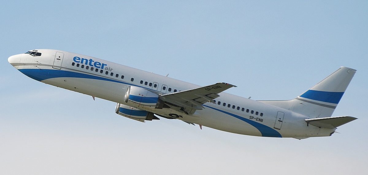
After takeoff, an aircraft needs to be able to climb quickly away from the runway into full flight and also be able to climb up to an initial cruising altitude at a reasonable rate. For an aircraft to climb, it takes more thrust and power over and above that for level flight at the same airspeed. Sufficient excess thrust and power margins must also be included in the event of a single engine failure to allow the aircraft to continue to climb. In the event of an engine failure called one engine inoperative (OEI), the aircraft must also be able to climb, albeit at reduced rates. Therefore, OEI performance considerations are always an essential part of the design of all multi-engine airplanes. OEI climb is particularly critical for twin-engine airliners, as shown in the photo below; they are designed to have much more significant amounts of excess thrust and power available from any one of the engines than would be used for three or four-engined airplanes.

For an airplane to climb, it must have excess power available over and above that required for level flight at the same weight, airspeed, and altitude.

As the airplane climbs higher and higher, its rate of climb will diminish because of the reduced thrust from the engines and the lower air density, and the values of the thrust (or power) required for flight and the thrust (or power) available begin to approach each other. Eventually, the rate of climb will reduce to the point that the aircraft can climb no higher for all practical purposes. This condition is called the operational flight ceiling. The estimation of the flight ceiling is also an essential part of the aircraft’s design, and sufficient excess thrust and power must be available to allow it to reach and cruise at an efficient operational altitude.

Learning Objectives

Understand the factors influencing an airplane’s climb rate and the time it takes to climb to altitude.
Use the basic equations for aircraft performance to set up and estimate an airplane’s climb rate under different flight conditions.
Appreciate the concept of a flight ceiling and the factors that will affect the attainable ceiling of an airplane.
Understand the principles of gliding flight and the significance of the lift-to-drag ratio in determining an aircraft’s gliding performance.

Steady Climbing Flight

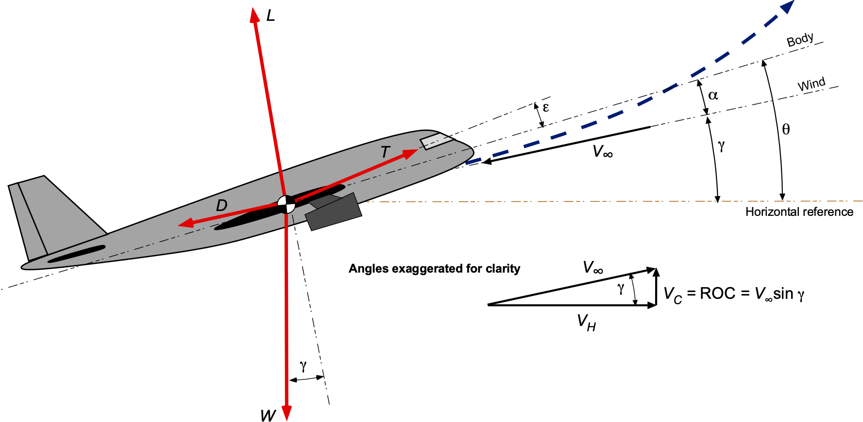
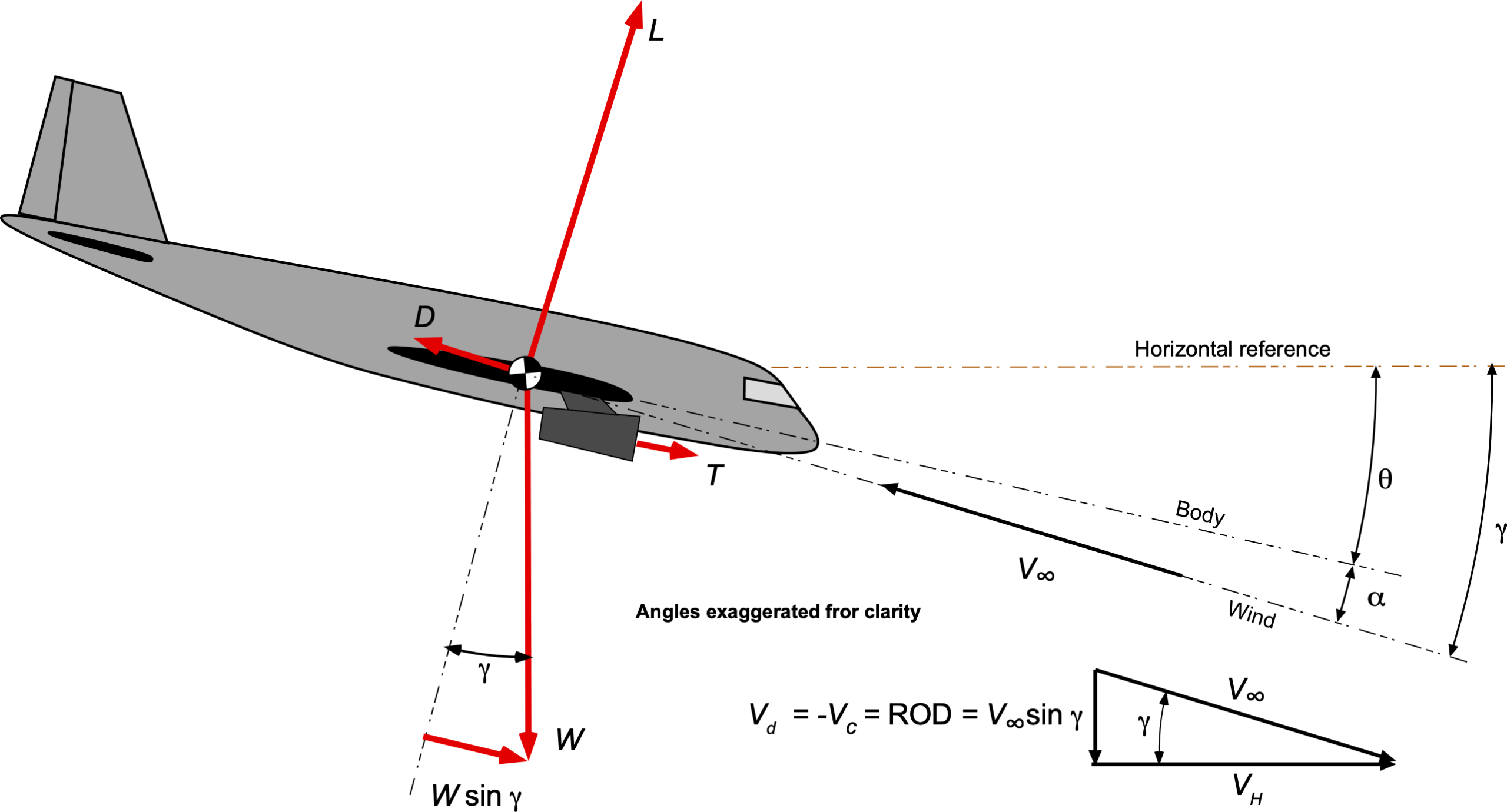
A schematic of an airplane in a climb is shown in the figure below. The pitch angle from the body reference axis relative to the horizontal reference is given the symbol $\theta$ , the angle of attack is $\alpha$ , and $\gamma$ is the climb or flight path angle. Notice that the angles are exaggerated here for clarity compared to what an average climb would look like. For descending or gliding flight, the value of $gamma$ would be negative, a condition considered later.

An airplane in a steady climb along a rectilinear flight path is typical of a standard operational climb.

The equations of motion are

(1) $\begin{equation*} \left( \frac{W}{g} \right) \frac{d V_{\infty}}{dt} = T \cos \epsilon - D - W \sin \gamma \end{equation*}$

and

(2) $\begin{equation*} \left(\frac{W}{g}\right) \frac{V_{\infty}^2}{r} = L + T \sin \epsilon \cos \phi - W \cos \gamma \end{equation*}$

For the steady, unaccelerated flight along a rectilinear flight path, then $dV_{\infty}/dt = 0$ and $V_{\infty}^2/r = 0$ (i.e., no radius of curvature), so the equations of motion reduce to

(3) $\begin{eqnarray*} T \cos \epsilon - D - W \sin \gamma & = & 0 \\[6pt] L + T \sin \epsilon - W \cos \gamma & = & 0 \end{eqnarray*}$

It can be further assumed that $\epsilon = 0$ , which means that the line of action of the thrust vector is along the direction of flight; this is a reasonable assumption. Therefore, the equations of static equilibrium further simplify to

(4) $\begin{eqnarray*} T - D - W \sin \gamma & = & 0 \\[6pt] L - W \cos \gamma & = & 0 \end{eqnarray*}$

The preceding equations for the climb condition are analogous to the results obtained for straight-and-level flight. However, notice that in a climb, for vertical equilibrium, the lift on the airplane’s wings is now slightly smaller than its weight because a small vertical component of the thrust from the propulsion system supports some of the airplane’s weight.

By multiplying the first of the preceding two equations by $V_{\infty}$ , then

(5) $\begin{equation*} T V_{\infty} = D V_{\infty} + W V_{\infty} \sin \gamma \end{equation*}$

and with rearrangement, then

(6) $\begin{equation*} \frac{T V_{\infty} - D V_{\infty}}{W} = V_{\infty} \sin \gamma \end{equation*}$

Notice that the vertical rate of climb $V_c$ is equal to $V_{\infty} \sin \gamma$ so that the rate of climb (ROC) is

(7) $\begin{equation*} \mbox{ROC} = V_c = V_{\infty} \sin \gamma = \frac{T V_{\infty} - D V_{\infty}}{W} \end{equation*}$

The abbreviations “ROC” or “R/C” are used variously in the literature on aircraft performance to denote the rate of climb.

The term $T V_{\infty}$ is the power available for flight $P_{\rm A}$ , and $D V_{\infty}$ is the power required $P_{\rm{req}}$ to overcome the drag of the aircraft. Therefore, the excess power available, $\Delta P$ , is

(8) $\begin{equation*} \Delta P = T V_{\infty} - D V_{\infty} = P_A - P_{\rm req} \end{equation*}$

so the ROC is then

(9) $\begin{equation*} \mbox{ROC} = V_c = \frac{\Delta P}{W} \end{equation*}$

It can be deduced then that the best climbing performance for an aircraft will be obtained at a low weight, with low drag, and with a large amount of excess power available. In this latter regard, excess power means the power available over and above required for straight-and-level flight at the same weight, airspeed, and density altitude. These former observations are certainly not unexpected based on physical reasoning.

Some aerodynamics can now be introduced into the analysis. In steady climbing flight, then

(10) $\begin{equation*} C_L = \frac{L}{\frac{1}{2} \varrho_{\infty} \, V_{\infty}^2 \, S} = \frac{W \cos \gamma}{\frac{1}{2} \varrho_{\infty} \, V_{\infty}^2 \, S} \end{equation*}$

and the standard drag polar for an airplane can be assumed, i.e.,

(11) $\begin{equation*} C_D = C_{D_{0}} + \frac{{C_L}^2}{\pi \, A\!R e} \end{equation*}$

Therefore, the total drag on the airplane is

(12) $\begin{equation*} D = \frac{1}{2} \varrho_{\infty} V_{\infty}^2 S \left( C_{D_{0}} + \frac{{C_L}^2}{\pi \, A\!R e} \right) \end{equation*}$

Substituting into the equation for the drag polar gives

(13) $\begin{equation*} D = \frac{1}{2} \varrho_{\infty} \, V_{\infty}^2 \, S \left( C_{D_{0}} + \frac{1}{\pi \, A\!R e} \right) \frac{(W \cos \gamma)^2}{\frac{1}{2} \varrho_{\infty} V_{\infty}^2 S} \end{equation*}$

After some rearrangement using the preceding results, solving for the rate of climb gives

(14) $\begin{equation*} \mbox{ROC} = V_c = V_{\infty} \left[ \frac{T}{W} - \frac{1}{2} \varrho_{\infty} \, V_{\infty}^2 \left( \frac{W}{S} \right)^{-1} C_{D_{0}} - \frac{W}{S} \left( \frac{2 \cos^2\gamma}{\varrho_{\infty} V_{\infty}^2 S \pi \, A\!R e} \right) \right] \end{equation*}$

Two critical parameters appear again, namely the wing loading of the airplane $W/S$ and its thrust-to-weight ratio $T/W$ , which will be seen to have primary dependencies on the airplane’s climb rate. Notice also that the rate of climb is improved with improved aerodynamic efficiency, i.e., with a lower value of $C_{D_{0}}$ and a higher value of $e$ .

There are no exact solutions to Eq. 14, but numerical and graphical solutions are possible. In part, closed-form solutions are impossible because engine performance (e.g., thrust and power) is often difficult to generalize through simple equations. However, estimating the climb rates is possible under certain assumptions. For example, because the climb angle is typically small for many classes of airplane, then $\cos^2\gamma \rightarrow 1$ , so the governing equation for the ROC becomes

(15) $\begin{equation*} V_c = V_{\infty} \left[ \frac{T}{W} - \frac{1}{2} \varrho_{\infty} \, V_{\infty}^2 \left( \frac{W}{S} \right)^{-1} C_{D_{0}} - \frac{W}{S} \left( \frac{2}{\varrho_{\infty} \, V_{\infty}^2 \pi \, A\!R e} \right) \right] \end{equation*}$

In the solution to this latter equation, the outcome is either:

The value of $V_c$ (the ROC) for a given value of $\gamma$ .
The value of $\gamma$ for a given value of $V_{\infty}$ .

Rate of Climb & Excess Power

It has been previously shown that the ROC of an airplane is proportional to the excess power available over and above that required for level flight, i.e.,

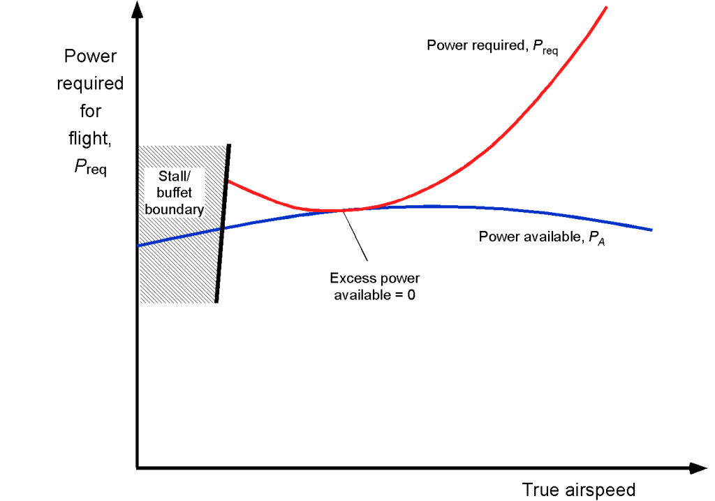
(16) $\begin{equation*} {\mbox ROC} = V_c = \frac{\Delta P}{W} \end{equation*}$

What this latter equation means, however, is that the ROC is related to the excess power available over and above that required for straight-and-level flight at the same weight $W$ , altitude, and airspeed $V_{\infty}$ . This outcome can be seen easily when the power required versus available power curves are plotted, which are shown in the figure below for a representative propeller-driven airplane.

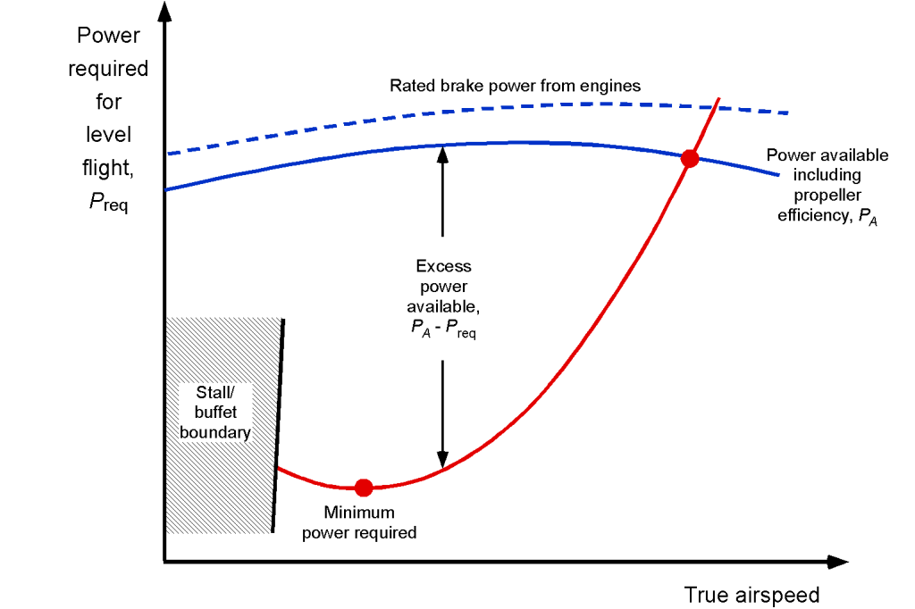
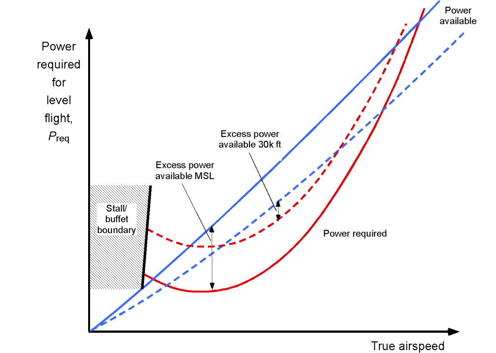
Representative power required versus power available curves for a propeller-driven airplane. The excess power available allows the aircraft to climb.

Remember that for a propeller-driven airplane, the power available is relatively constant over a wide range of airspeeds. Still, for a jet where $T$ is nominally constant, the power available (i.e., the useful power or $T V_{\infty}$ ) increases linearly with airspeed, as shown in the figure below. Therefore, it can be concluded that the propeller and jet airplanes will have markedly different rates of climb characteristics.

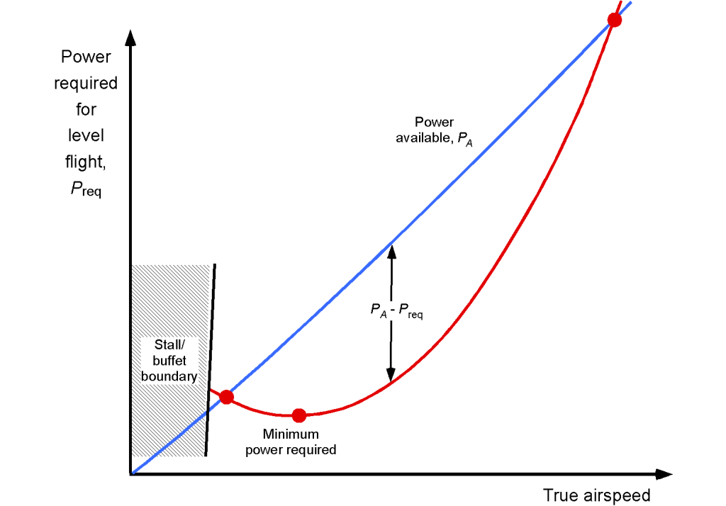
Representative power required versus power available curves for a jet airplane. Notice that compared to a propeller-driven airplane, there is significantly less excess power available at low airspeeds.

In each case, however, the ROC depends on the excess power available, for example, the resulting climb characteristics shown in the figure below, both for propeller-powered and jet airplanes. Jets have relatively low amounts of excess power available at lower airspeeds so that they can achieve only relatively low climb rates at low airspeeds, i.e., just after takeoff.

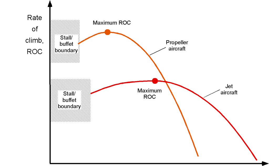
Representative rate of climb curves for a propeller-driven airplane versus a jet airplane.

Again, it is apparent that the maximum rate of climb, ROC $_{\rm max}$ , occurs where the excess power available $\Delta P$ is the greatest. Because of the larger excess power available with propeller-driven airplanes at low airspeeds, they generally have excellent climb characteristics just after takeoff. They are ideally suited for operations from shorter runways or runways surrounded by mountainous terrain.

Jet aircraft exhibit characteristics where the most significant climb rates are obtained at higher airspeeds. For example, when observing an airliner taking off, it will be noted that it first climbs relatively slowly until airspeed has built sufficiently and the undercarriage and flaps have been retracted to reduce drag before the best climb rates are possible. Long-haul commercial airliners, which are laden with fuel, often have rates of climb that are less than 500 ft/min until airspeed builds and the aircraft exits the terminal airspace. The resulting climb to the cruise altitude is usually performed in stages, where fuel must be burned off to decrease the in-flight weight and allow a climb to a higher altitude.

Worked Example #1 – Estimating the maximum possible rate of climb

An airplane with fuel has an in-flight weight of 2,550 Ib. The wing area, $S$ , is 174 ft² and the wingspan, $s$ , is 36 ft. The Oswald efficiency factor, $e$ , is 0.7, and the zero-lift drag coefficient $C_{D_{0}}$ = 0.0319. The engine brake power available at sea level is 180 hp, and the propeller efficiency, $\eta_p$ , is 80%. Assume that the airplane is flying at standard sea level conditions at an airspeed of 95 kts. Estimate the maximum possible rate of climb.

The lift coefficient of the wing is

$C_L = \frac{2 W}{\varrho_{\infty} \, V_{\infty}^2 \, S}$

An airspeed of 95 kts is equal to 160.34 ft/s. Therefore, at MSL ISA

$C_L = \frac{2 \times 2,550}{0.002378 \times (160.34)^2 \times 174.0} = 0.48$

The wing aspect ratio is

$A\!R = \frac{s^2}{S} = \frac{36.0^2}{174.0} = 7.45$

Therefore, the drag coefficient on the aircraft is

$C_D = C_{D_{0}} + \frac{C_L^2}{\pi \, A\!R \, e} = 0.0319 + \frac{0.48^2}{\pi \times 7.45 \times 0.7} = 0.046$

The drag on the aircraft is

$D = \frac{1}{2} \varrho_{\infty} V_{\infty}^2 \, S \, C_D = 0.5 \times 0.002378 \times (160.34)^2 \times 174.0 \times 0.046 = 244.67~\mbox{lb}$

The ideal power required for straight and level flight is

$P_{\rm req} = D \, V_{\infty} = 244.67 \times 160.34 = 39,230.4~\mbox{ft-lb/s} = 71.33~\mbox{hp}$

Therefore, the maximum rate of climb will depend on the excess power available, which is

$V_{c_{\rm max}} = \frac{\eta_p \, \Delta P}{W} = \frac{0.8 \times 550 \times (180.0 - 71.33)}{2,550} = 18.76~\mbox{ft/s} \approx 1,125~\mbox{ft/min.}$

Hodograph Method

A graphical method often used for solving the climb rate is called the hodograph method. A hodograph is a diagram, as shown below, which gives a vectorial visual representation of a point in space; it is the locus of one end of a variable vector with the other end fixed at the origin (0,0) of the graph. In this method, the vertical speed or ROC or $V_c = V_{\infty} \sin \gamma$ is plotted versus the horizontal speed $V_H = V_{\infty} \cos \gamma$ , which gives a locus of points that is called a hodograph. As shown in the figure below, a horizontal tangent to the hodograph provides the maximum rate of climb. Also, any line from the graph’s origin to a point on the hodograph gives the angle of climb, and the length of this line will be the corresponding airspeed $V_{\infty}$ .

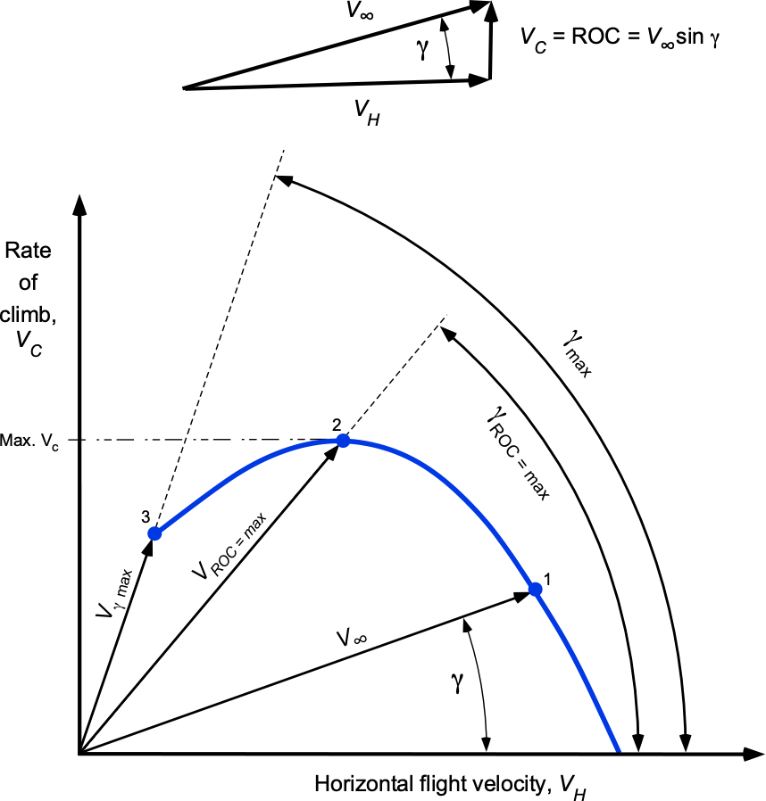
Moving along the hodograph in a continuous counterclockwise direction leads to the following observations:

The value of $V_c$ first increases, and $V_{\infty}$ decreases.
There comes a point where $V_c$ reaches a maximum (point 2). $V_c$ begins to decrease and reaches a tangent to the curve (point 3), which is the steepest climb angle.
The maximum or steepest climb angle does not occur at the same airspeed as the maximum rate of climb.

Why are both the maximum angle of climb and the maximum rate of climb important?
The airspeed for the best climb angle, also known as $V_x$ , is the airspeed that allows an aircraft to gain the most altitude in the shortest possible distance over the ground, e.g., for obstacle or terrain avoidance. The best angle of climb airspeed occurs when the difference between the power available and the power required is greatest. The best rate of climb, also known as $V_y$ , is beneficial when the aircraft needs to achieve the highest climb rate possible. A high climb rate is helpful because it quickly allows the aircraft to reach higher operational altitudes more efficiently.

Effects of Altitude

Both weight and altitude (i.e., density altitude) will affect an aircraft’s climb rate. Because the effects of changes in altitude are more important than changes in weight after the aircraft first takes off and burns off much fuel weight, it is logical to examine altitude effects on climb performance. Recall that the possible rate of climb is proportional to the excess power available over and above required for straight-and-level flight at the same altitude. The figure below shows representative results for the power needed in a propeller-driven airplane with increasing altitude.

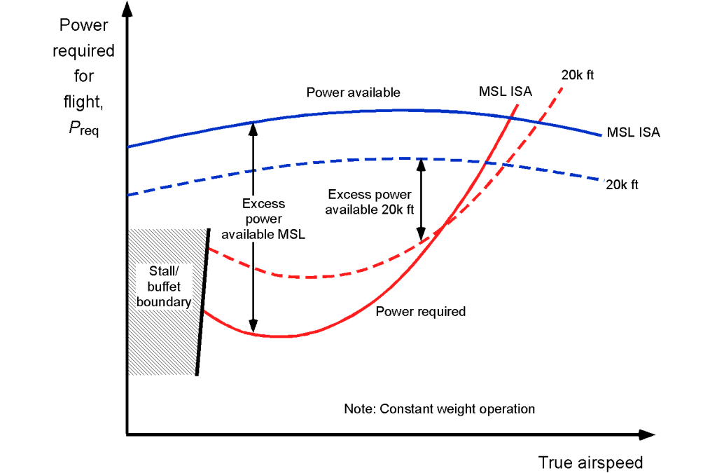
The power required varies according to the relationship for a propeller-driven airplane, i.e.,

(17) $\begin{equation*} P_{\rm req_{\rm alt}} = P_{\rm req_{\rm MSL}} \left( \frac{\varrho_0}{\varrho} \right) \end{equation*}$

which shows that the power requirements increase significantly with altitude. However, the advantage of flying at a higher altitude is that the drag on the aircraft is less, so for the same power, the aircraft will be able to fly at a higher airspeed.

The corresponding behavior for a jet aircraft is shown in the figure below. Again, the thrust and the power available are also affected by altitude, dropping off quickly above a certain altitude. The reduction or lapse in engine power depends, of course, on the particular characteristics of the engine and propulsion system. Therefore, the excess power available (to climb) diminishes with altitude because of these preceding effects, i.e., more power is required for flight, and less power is available for flight. When the power required is equal to the power available at a given altitude, the aircraft reaches its maximum attainable airspeed. Furthermore, the aircraft cannot climb at any airspeed without excess power.

The excess power available to climb diminishes at higher altitudes as the gap narrows between the required and available power.

Determining Rates of Climb

Previously, it was shown that the governing equation for the ROC is

(18) $\begin{equation*} V_c = V_{\infty} \left[ \frac{T}{W} - \frac{1}{2} \varrho_{\infty} \, V_{\infty}^2 \left( \frac{W}{S} \right)^{-1} C_{D_{0}} - \frac{W}{S} \left( \frac{2 }{\varrho_{\infty} \, V_{\infty}^2 \pi \, A\!R \, e } \right) \right] \end{equation*}$

Given a value of airspeed $V_{\infty}$ , the corresponding $V_c$ and the climb angle is

(19) $\begin{equation*} \sin \gamma = \frac{V_c}{V_{\infty}} \end{equation*}$

or from Eq. 18 simply by dividing by $V_{\infty}$ then

(20) $\begin{equation*} \sin \gamma = \frac{T}{W} - \frac{1}{2} \varrho_{\infty} \, V_{\infty}^2 \left( \frac{W}{S} \right)^{-1} C_{D_{0}} - \frac{W}{S} \left( \frac{2}{\varrho_{\infty} \,V_{\infty}^2 \pi \, A\!R \, e} \right) \end{equation*}$

Also, it is clear that

(21) $\begin{equation*} V_{\infty} \sin \gamma = \frac{T V_{\infty} - D V_{\infty}}{W} \end{equation*}$

or

(22) $\begin{equation*} V_{\infty} \sin \gamma = V_{\infty} \left( \frac{T - D}{W} \right) \end{equation*}$

and

(23) $\begin{equation*} \sin \gamma =\frac{T}{W} - \frac{D}{W} \end{equation*}$

So, the rate of climb increases with higher thrust values and a reduction of drag and weight, as expected.

To find the maximum angle of climb then, the result that $L = W \cos \gamma$ is used, and so

(24) $\begin{equation*} \sin \gamma = \frac{T}{W} - \frac{\cos \gamma}{L/D} \end{equation*}$

Typically, the maximum angle of climb would be used on takeoff to clear an obstacle at the end of the runway. Most airliners will be flown just after takeoff at airspeed for the maximum climb angle. When terrain clearance is assured, the aircraft’s pitch angle can be lowered, and the airspeed increased to give a better rate of climb. Assuming again that $\gamma$ is small such that $\cos \gamma =1$ , then

(25) $\begin{equation*} \sin \gamma = \frac{T}{W} - \frac{1}{L/D} \end{equation*}$

showing that the climb angle depends on the airplane’s lift-to-drag ratio $L/D$ .

Consider first a jet airplane (for which thrust is essentially constant at all airspeeds), then the maximum angle of climb $\gamma_{\rm max}$ is achieved at the maximum value of the lift-to-drag ratio, i.e.,

(26) $\begin{equation*} \sin \gamma_{\rm max} = \frac{T}{W} - \frac{1}{(L/D)_{\rm max}} \end{equation*}$

For a jet aircraft, it can be shown that the maximum lift-to-drag occurs at the condition

(27) $\begin{equation*} (L/D)_{\rm max} = \sqrt{\frac{1}{4 C_{D_{0}} K}} \end{equation*}$

where $K$ is given by

(28) $\begin{equation*} K = \frac{1}{\pi \, A\!R e} \end{equation*}$

so

(29) $\begin{equation*} \sin \gamma_{\rm max} = \frac{T}{W} - \sqrt{ \frac{1}{4 C_{D_{0}} K}} \end{equation*}$

From these results, the airspeed corresponding to the maximum climb angle can be found, which is

(30) $\begin{equation*} V_{\gamma_{\rm max}} = \sqrt{ \frac{2}{\varrho} \left( \frac{K}{C_{D_{0}} }\right)^{1/2} \left( \frac{W}{S} \right) \cos \gamma_{\rm max}} \end{equation*}$

The conditions for the maximum rate of climb can also be estimated analytically.

For a propeller airplane, the power required is

(31) $\begin{equation*} P = \frac{T_A V_{\infty}}{\eta_p} \end{equation*}$

and the power available is equal to the power required, so

(32) $\begin{equation*} P_A = \eta_p P \end{equation*}$

and this power is assumed to be constant with both airspeed and rate of climb. In this case, then

(33) $\begin{equation*} \sin \gamma = \frac{\eta_p P}{V_{\infty} W} - \frac{1}{2} \varrho_{\infty} V_{\infty}^2 \left( \frac{W}{S} \right)^{-1} C_{D_{0}} - \frac{W}{S} \frac{2K}{\varrho_{\infty} V_{\infty}^2} \end{equation*}$

By differentiating this latter equation with respect to $V_{\infty}$ and setting equal to zero for a maximum, then with some algebra, it is possible to show that

(34) $\begin{equation*} V_{\gamma_{\rm max}} = \frac{ 4 (W/S) K}{\eta_p \, \varrho_{\infty} \, (P/W)} \end{equation*}$

for a typical propeller airplane. Again, the maximum rate of climb conditions can also be estimated analytically.

Accelerated Climb

In this case, the airplane accelerates along the direction of the flight path. Therefore, the equation of motion is

(35) $\begin{equation*} T - D - W \sin \gamma = \left( \frac{W}{g} \right) a \, g \end{equation*}$

where the acceleration is $a\, g$ . Therefore,

(36) $\begin{equation*} T = D - W \left( \frac{V_c}{V_{\infty}} \right) + W \, a \end{equation*}$

and so the power required in this case is

(37) $\begin{equation*} P_{\rm req} = T V_{\infty} = D V_{\infty} + W \left( V_c + a V_{\infty} \right) = D V_{\infty} + W \, V_c + W a V_{\infty} \end{equation*}$

with $W a V_{\infty}$ being the extra power required to accelerate in the climb.

Time to Climb

The time it takes to climb from one altitude to another is also of consideration, i.e., to climb from an altitude $h = h_1$ to altitude $h = h_2$ . This latter characteristic is important in operational service when an aircraft may be required to climb to a certain altitude in a given time, such as to comply with air traffic requirements, i.e., to fit in with flight routings or for collision avoidance. It is also more efficient for an aircraft to fly at higher altitudes (the drag is less to the thrust or power required is less), so the ability to climb quickly to an efficient cruising altitude is important. Just after takeoff, an airliner is laden with fuel and relatively heavy, affecting its best rate of climb and airspeed for the best rate of climb.

The rate of climb is the vertical component of the airspeed, so

(38) $\begin{equation*} \frac{dh}{dt} = V_{\infty} \sin \gamma = V_c \end{equation*}$

or

(39) $\begin{equation*} dt = \frac{dh}{V_c} \end{equation*}$

where $V_c$ would be a function of weight and altitude. This result means that the time to climb from $h_1$ to $h_2$ would be

(40) $\begin{equation*} t = \int_{h_1}^{h_2} \frac{dh}{V_c} \end{equation*}$

The minimum time to climb would be obtained at the maximum rate of climb so that the time would be

(41) $\begin{equation*} t_{\rm min} = \int_{h_1}^{h_2} \frac{dh}{V_{c_{\rm max}}} \end{equation*}$

Worked Example #2 – Time to climb

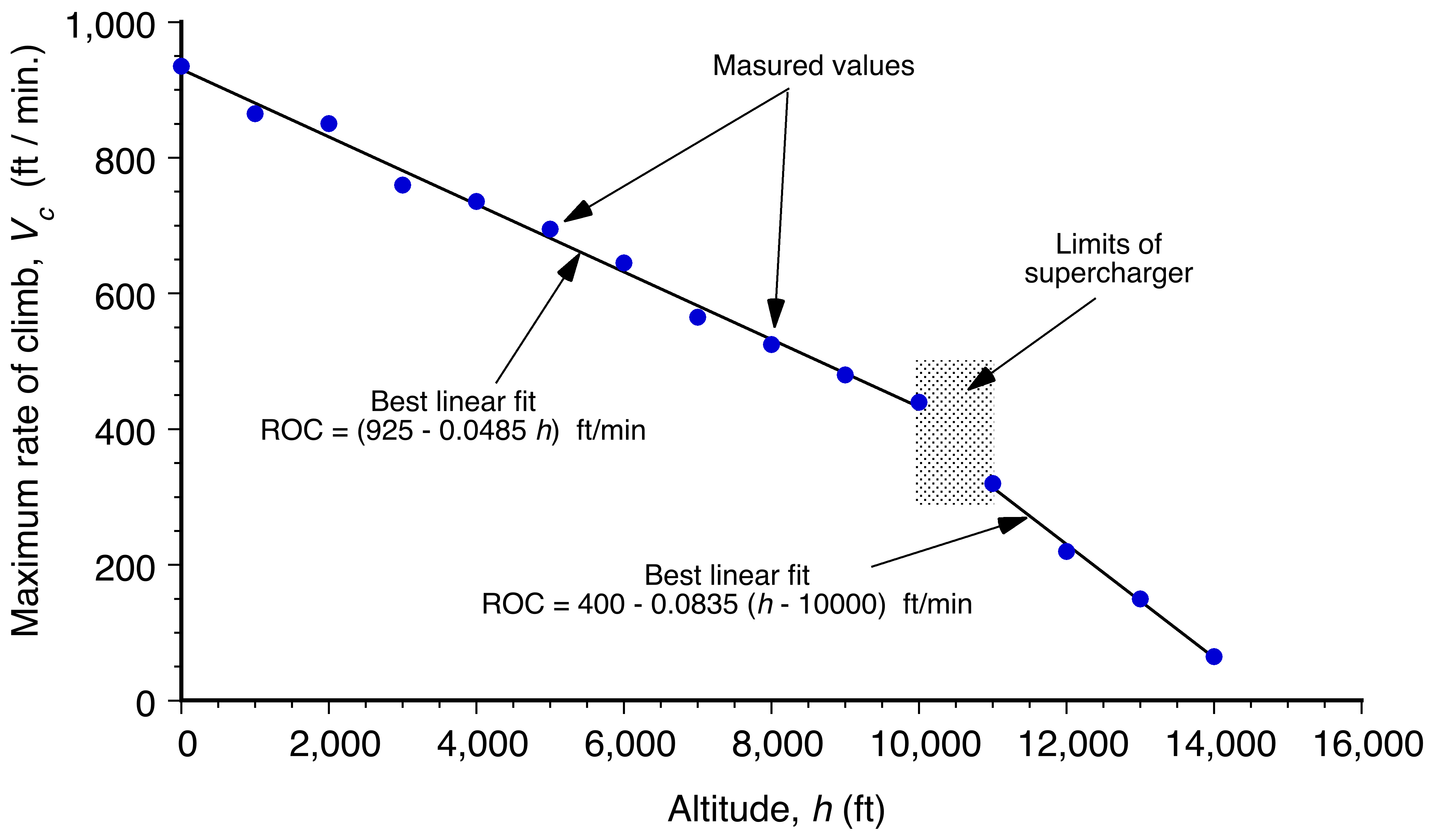
The maximum rate of climb performance of a high-performance single-engine airplane is determined from the flight test measurements, as shown in the figure below. Estimate the minimum time taken for the aircraft to climb from 1,000 ft to 9,000 ft.

The change in altitude $\Delta h$ , for a given maximum rate of climb $V_c$ , over a period $t_{\rm min}$ , can be estimated using

$\Delta h = \int_0^{t_{\rm min}} V_c \, dt$

which is simply the area under the rate of climb versus time curve (line). In this case, because the aircraft is below 10,000 ft, then

$\Delta h = \int_0^{t_{\rm min}} \left( 925 - 0.0485 \, \Delta h \right) \, dt$

where $h$ is 1,000 ft at $t$ = 0, and $h$ is 9,000 ft at $t = t_{\rm min}$ . Performing the integration gives

$\Delta h = \left( 925 - 0.0485 \, \Delta h \right) t_{\rm min}$

so that

$t_{\rm min} = \frac{\Delta h}{\left( 925 - 0.0485 \, \Delta h \right)}$

In this case, $\Delta h$ = 8,000 ft, so inserting the numbers gives

$t_{\rm min} = \frac{9,000 - 1,000}{925 - 0.0485 (9,000 - 1,000)} = \frac{8,000 }{925 - 0.0485 \times 8,000} \approx 15~\mbox{mins.}$

Ceiling

The airplane’s absolute ceiling is defined as the altitude for which the rate of climb approaches zero, i.e., $V_c \rightarrow 0$ . In this regard, the excess power available over and above that required for straight-and-level flight at the same weight, airspeed, and altitude diminishes to zero, as shown in the figure below. The service ceiling is defined as the altitude where the rate of $V_c$ reduces to 100 ft/min. It is a more useful measure of the ceiling because it represents the upper limit for level flight.

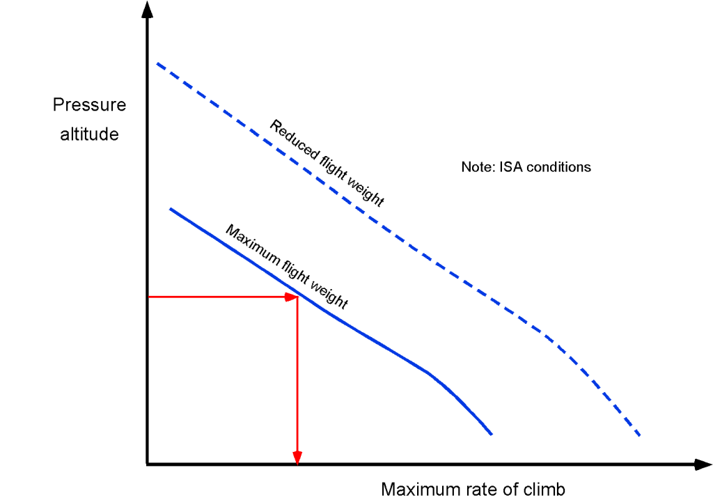
The service and absolute ceilings can be determined as follows:

Calculate the rate of climb at a given weight for different altitudes, which can be done graphically or numerically using the hodograph method.
Plot the results as a curve in terms of altitude versus the achievable rate of climb, as shown in the figure below.
As the rate of climb diminishes toward a lower threshold, cease the calculations and extrapolate the resulting curve to find the value of altitude when $V_c$ = 100 ft/min, which is the service ceiling.
Extrapolate the curve to find the height value at $V_c$ = 0, which is the aircraft’s absolute ceiling beyond which it cannot climb (at the given weight).

This latter approach is tedious but effective. Another method is to set $V_c$ equal to zero in Eq. 18 and solve for the air density, which can then be related to pressure altitude using the equations of the ISA.

Determining the maximum possible rate of climb at different altitudes allows for an estimation of both the service ceiling and the absolute ceiling for the airplane. The results will be a function of aircraft weight.

Notice that a structural pressurization limit may also set an aircraft’s ceiling because the fuselage is a large pressure vessel. For example, a commercial jet airliner is generally limited to altitudes less than 41,000 ft, even though it may have sufficient excess power to climb higher. This characteristic is because the pressure differential between the cabin and the external ambient pressure becomes large enough for the fuselage to reach structural stress limitations.

Worked Example #3 – Estimating the flight ceiling

Determine the service and absolute ceilings for the single-engine aircraft considered in worked example #2. Notice that the rate of climb (ROC) in feet per minute (ft/min) above 10,000 ft is reduced because of engine power lapse. How long will it take for the aircraft to climb from its service ceiling to its absolute ceiling?

The rate of climb above 10,000 ft is

$V_c = 400 - 0.0835 \left( h - 10,000 \right)$

and rearranging to solve for $h$ gives

$h = \frac{400 - V_c}{0.0835} +10,000$

The service ceiling is when $V_c$ approaches 100 ft/min, so

$h_{\rm sc} = \frac{400 - 100}{0.0835} +10,000 = 13,593~\mbox{ft}$

The absolute ceiling is when $V_c$ approaches 0 ft/min, so

$h_{\rm ac} = \frac{400 - 0}{0.0835} +10,000 = 14,790~\mbox{ft}$

The time to climb between the service ceiling and the absolute ceiling will be

$t_{\rm climb} = \frac{\Delta h}{\left( 400 - 0.0835 \, \Delta h \right)}$

In this case, $\Delta h$ = 14,790 – 13,593 = 1,197 ft, so inserting the numbers gives

$t_{\rm climb} = \frac{1,197 }{400 - 0.0835 \times 1,197} \approx 4~\mbox{mins.}$

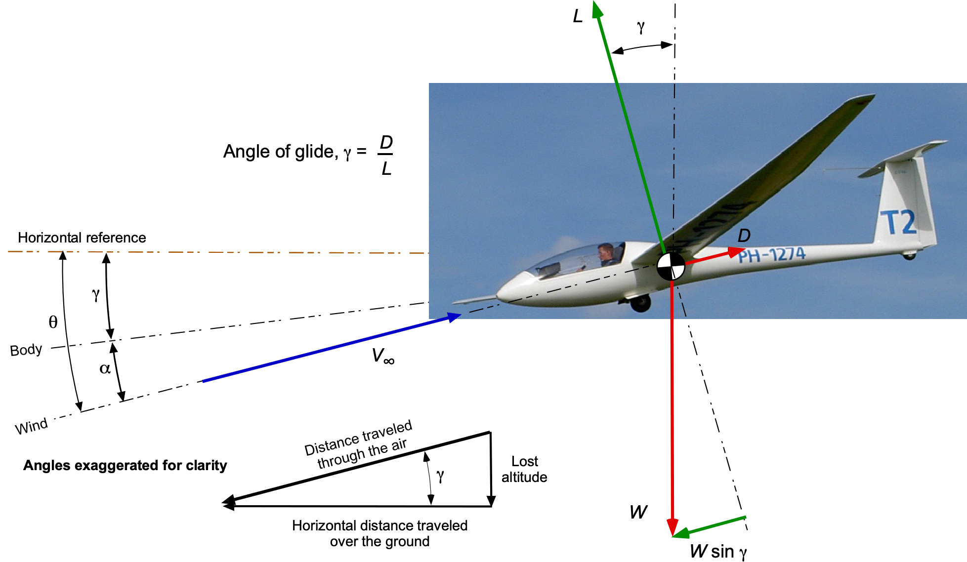
Gliding Flight

Consider now an airplane in power-off gliding flight, as shown in the figure below. In this case, the powerplant(s) thrust, $T$ , is zero. However, in the zero thrust condition, the engine may produce drag (e.g., from a windmilling or feathered propeller). It must be factored into the total drag of the airplane and, hence, the resulting glide performance. The glide angle is denoted by $\gamma$ .

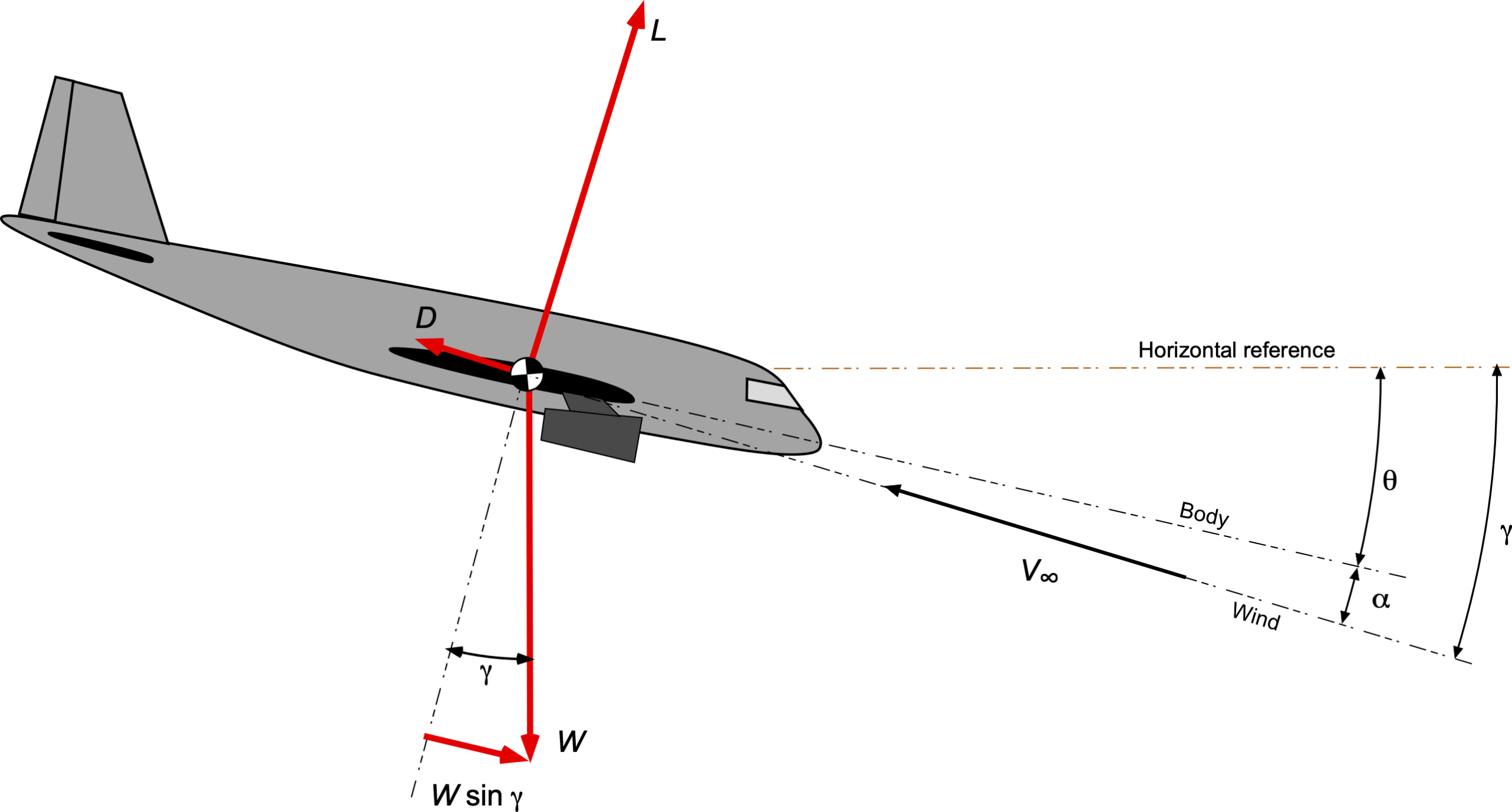In this case, the equations of motion reduce to

(42) $\begin{eqnarray*} D & = & W \sin \gamma \\[6pt] L & = & W \cos \gamma \end{eqnarray*}$

Dividing one equation by the other gives

(43) $\begin{equation*} \frac{\sin \gamma}{\cos \gamma} = \tan \gamma = \frac{1}{L/D} \end{equation*}$

which shows that the glide angle $\gamma$ will be a function only of the lift-to-drag ratio $L/D$ . The higher the $L/D$ , the shallower the glide angle and the further the glide distance from a given height. The shallowest glide ratio will be obtained at the maximum value of $L/D$ , i.e.,

(44) $\begin{equation*} \gamma_{\rm min} = \tan^{-1} \left( \frac{1}{L/D_{\rm max}} \right) \end{equation*}$

Proceeding further by considering the aerodynamics in the glide gives for lift

(45) $\begin{equation*} L = W \cos \gamma = \frac{1}{2} \varrho_{\infty} \, V_{\infty}^2 \, S \, C_L \end{equation*}$

and solving for the airspeed gives

(46) $\begin{equation*} V_{\infty} = \sqrt{ \frac{2 \cos \gamma}{\varrho_{\infty} \, C_L} \left( \frac{W}{S} \right) } \end{equation*}$

where the familiar wing loading term $W/S$ appears once again in the results.

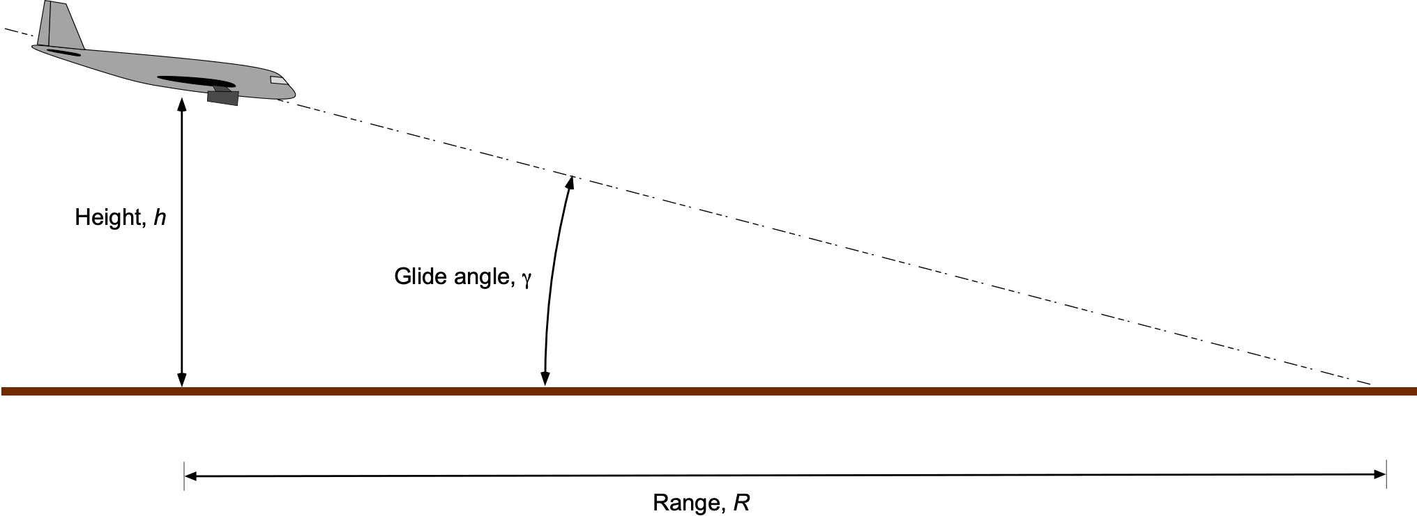
This result tells us that the higher the wing loading, the higher the expected glide speed, which also depends on density altitude. The glide angle remains a function of the $L/D$ , but the rate of descent will be higher at a higher gliding airspeed. This means the airplane will cover the same distance over the ground (i.e., the gliding distance) but reach the ground sooner with a higher airspeed. The range $R$ from a given altitude $h$ is easily calculated because

(47) $\begin{equation*} R = \frac{h}{\tan \gamma} = h \left( \frac{L}{D} \right) \end{equation*}$

as shown in the figure below.

Gliding distance from a given altitude depends on the airplane’s aerodynamic efficiency (i.e., the lift-to-drag ratio) and the airspeed at which it is flown.

Worked Example #4 – Estimating glide distance after fuel exhaustion

A jet airplane with a best $L/D$ of 15 at 195 knots is initially at 30,000 ft altitude above the ground and suffers a complete power failure after a fuel leak causes it to run out of fuel. Estimate the approximate gliding distance at the best glide airspeed and how long it will take to reach the ground.

The distance or range, $R$ , it can glide will be

$R = h_{\rm init} \left( \frac{L}{D} \right)$

where in this the the initial height, $h_{\rm init}$ , is 30,000 ft. Inserting the numbers gives

$R = 30,000 \left( 15 \right) = 450,000 ~\mbox{ft} \approx 74~\mbox{nautical miles}$

This latter result gives some comfort in that the loss of total power in an airliner (which is not unheard of) provides the pilot with a considerable gliding distance to reach an airfield. However, to achieve a specific $L/D$ , the airplane must fly at a particular airspeed, called the equilibrium glide speed. Recall that both $C_L$ and hence $L/D$ (or $C_L/C_D$ ) depend on airspeed. Distance is velocity times time, so in this case, the time it takes to reach the ground will be

$t \approx \frac{74}{195} = 0.38~\mbox{hrs} \approx 8.6~\mbox{minutes}$

This is not long, and the pilots must act quickly to safely land the aircraft at the nearest airfield. It can be done! It has been done!

Sailplanes & Gliders

These preceding aerodynamic principles are also fundamental to the sport of gliding. To be able to glide long distances from a given altitude depends on the ability of a sailplane (a high-performance glider capable of efficient soaring flight) to have a high lift-to-drag ratio and shallow glide angles $\gamma$ . To sustain flight, a sailplane can use rising air currents from thermals, uplifted air when the wind blows against hills and ridges, sea-breeze frontal boundaries, or atmospheric waves.

As will be apparent from the figure below, gravity provides the component of weight needed to overcome the drag in a glide. For the shallow angles of glide typical of a sailplane, then

(48) $\begin{equation*} \gamma = \tan^{-1} \left( \frac{D}{L}\right) \approx \frac{1}{L/D} \end{equation*}$

Therefore, the shallowest glide angle will be obtained at the maximum value of the lift-to-drag ratio, $L/D$ . While gliders and sailplanes are basically the same, sailplanes usually have $L/D$ values exceeding 30:1.

The balance of forces on a sailplane shows that the higher the lift-to-drag ratio of the aircraft, the shallower the glide angle.

High aerodynamic efficiency is essential for good gliding performance, so gliders have different aerodynamic features not found in other aircraft. For example, the wings of a modern glider use smooth, low-drag laminar airfoils. The wings are made of composite materials with great geometric accuracy, and the surfaces are made glassy smooth by polishing. Sailplanes may also use winglets to decrease drag further and improve the wing’s aerodynamic efficiency by reducing induced drag. In addition, the hinge gaps of the ailerons, rudder, and elevator are carefully sealed on sailplanes to reduce drag further. A better lift-to-drag ratio or $L/D$ means a sailplane can glide further from a given altitude, as shown in the figure below.

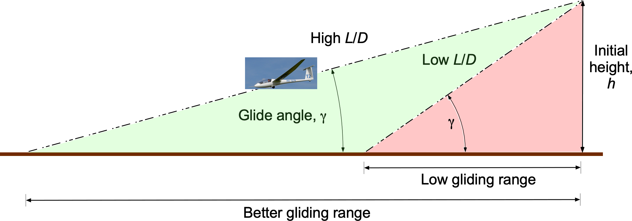A sailplane with a better lift-to-drag ratio $L/D$ can glide further.

Not only is the maximization of the $L/D$ of a sailplane important but in competitions where both distance and speed are essential, the best $L/D$ must be obtained at relatively high airspeeds. This latter result can be seen from the gliding polar; an example being shown below. In this case, the polar is a hodograph for descending flight, the airspeed along the flight path being $V_H$ and $V_c$ being negative, so the rate of descent, $V_d$ , in this case. Notice that the best glide ratio is obtained when the straight line from the graph’s origin at (0,0) touches at a tangent to the polar.

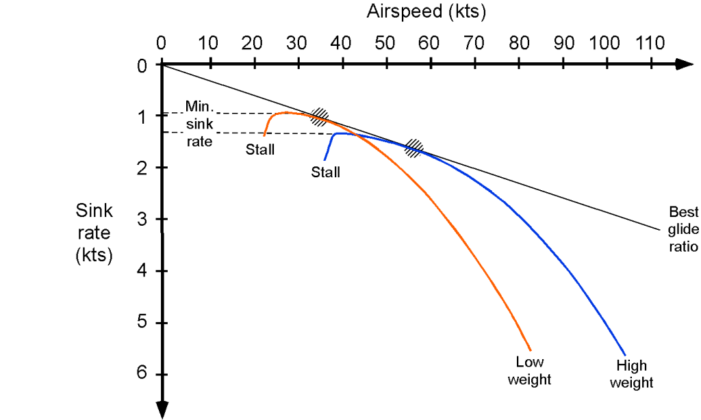
Notice also that the best glide ratio is obtained at a higher airspeed when the sailplane is flown at a higher weight. Because the gliding airspeed is a function of wing loading, all things being equal, a sailplane with a higher wing loading will be able to glide at a higher airspeed and travel further in a given time. In this regard, modern competition gliders carry jettisonable water ballast in the wings. The water ballast’s extra weight is advantageous if the strong thermals and soaring conditions allow the sailplanes to climb in rising air. Although heavier gliders have a slight disadvantage when climbing in thermals, they can achieve a higher airspeed at any given glide angle. This latter characteristic is advantageous in strong updraft conditions when sailplanes spend only a small amount of time climbing in thermals. The pilot can jettison the water ballast at any time and usually before landing to minimize landing loads on the airframe.

Worked Example #5 – Gliding range of a sailplane

The pilot of a sailplane is at an altitude of 3,500 ft MSL and needs to glide about 20 nautical miles to an airfield at 100 ft MSL. The sailplane has a maximum lift-to-drag ratio, $L/D$ , of 30:1. Assuming still air, will the pilot make it to the airfield in a single glide? If not, how high will the sailplane have to be before setting out on the final glide?

The steady gliding range, $R$ , from a given initial altitude, $h$ , can be calculated using

$R = h \left( \frac{L}{D} \right)$

So from 3,500 ft, the gliding distance will be

$R = \left( 3,500 - 100 \right) \times 30.0 = 102,000~\mbox{ft} \approx 16.8~\mbox{nautical miles}$

Therefore, the sailplane is not high enough to reach the airfield in a single glide. To make the airfield, the pilot must find a thermal or other lift to reach a slightly higher altitude. This altitude is

$h_{\rm ref} = \frac{R}{L/D} = \frac{20}{30} = 0.67~\mbox{nautical miles} \approx 4,100~\mbox{ft}$

Of course, this is the minimum altitude, and the pilot would want to have about another 1,000 ft of altitude to be sure of getting to the airfield and setting up for a landing.

Summary & Closure

Establishing the climbing performance of an aircraft is fundamental to its overall flight capability. The ability to take off from a runway and establish a sufficient angle of climb or rate of climb to clear obstacles is an essential consideration in the design process. The rate of climb for any given aircraft is a function of its excess power available over and above that needed for level flight at a given weight and operating density altitude. Climb capability is crucial for one engine inoperative (OEI) conditions, and sufficient power must still be available from the remaining engine(s) to permit a safe rate of climb.

Propeller-driven airplanes tend to have significant excess power available at low airspeeds. They generally have impressive short takeoff and high initial rates of climb compared to jets, so they are ideal for use on short runways or those surrounded by high terrain. Jets, however, have relatively low amounts of excess power available at lower airspeeds, and initial climb performance is much lower. The maximum attainable altitude of an aircraft will also be limited by the excess power available; power will diminish with increasing density altitude, so there comes the point where the excess power available diminishes so that the aircraft cannot climb any higher, referred to as the ceiling.

The ability to glide to a safe landing with complete power loss is also fundamental to the safe design of all aircraft. While powered aircraft rarely make good gliders, the ability to land without power is always a consideration for all aircraft types regarding flight safety. One has to hope it never happens, but cases of fuel exhaustion are not unheard of, even in commercial operations.

5-Question Self-Assessment Quickquiz

For Further Thought or Discussion

Explain why an airplane’s maximum climb rate depends on density altitude.
An airliner typically climbs to its maximum cruising altitude in several stages. Explain why this process is required.
After takeoff from a valley surrounded by mountainous terrain, will an airplane need to climb at its best angle or best rate? Discuss.
Would a propeller or jet aircraft be preferred for operations out of smaller airports surrounded by mountains, and why?
Discuss the trade-offs in selecting a steeper climb angle versus a shallower climb angle during takeoff and climb, considering factors such as fuel efficiency, engine stress, and passenger comfort.
Explain the concept of rate of climb versus angle of climb and how they relate to an aircraft’s performance.
Discuss the impact of engine performance degradation or failure on an airplane’s ability to climb and how pilots manage such situations.
In competition gliding, a sailplane may often carry jettisonable water ballast. Why?

Other Useful Online Resources

To dive further into the climbing and gliding characteristics of aircraft, visit the following websites:

FAA Pilot’s Handbook of Aeronautical Knowledge. The Federal Aviation Administration (FAA) publishes a comprehensive guide for pilots, and Chapter 7 explicitly covers the aerodynamics of flight, including climb performance. You can access it online in PDF format here.
This online resource provides an in-depth guide on airplane performance, including climb performance. It covers various topics such as takeoff and climb performance charts, factors affecting climb rate, and techniques for optimizing climb performance. You can find it here.
Skybrary’s entry on gilding includes a link to a report on a successful glide descent to a landing in an Airbus A330 after it ran out of fuel.
How Stuff Works article on how far a plane can glide after engine failure.

License

Icon for the Creative Commons Attribution-NonCommercial-NoDerivatives 4.0 International License

Introduction to Aerospace Flight Vehicles Copyright © 2022, 2023, 2024 by J. Gordon Leishman is licensed under a Creative Commons Attribution-NonCommercial-NoDerivatives 4.0 International License, except where otherwise noted.

Digital Object Identifier (DOI)

https://doi.org/https://doi.org/10.15394/eaglepub.2022.1066.n38