36
Introduction
When a freestream flow approaches a finite wing, characterized by a definitive span from tip to tip, the downstream flow develops a trailing wake system containing swirling flows known as wingtip vortices, as shown in the figure below. These vortices induce a vertical downwash velocity over the wing’s surface, particularly near the wing tips.[1] This downwash reduces the effective angle of attack of the wing, diminishes the lift, and increases drag, which is called induced drag.
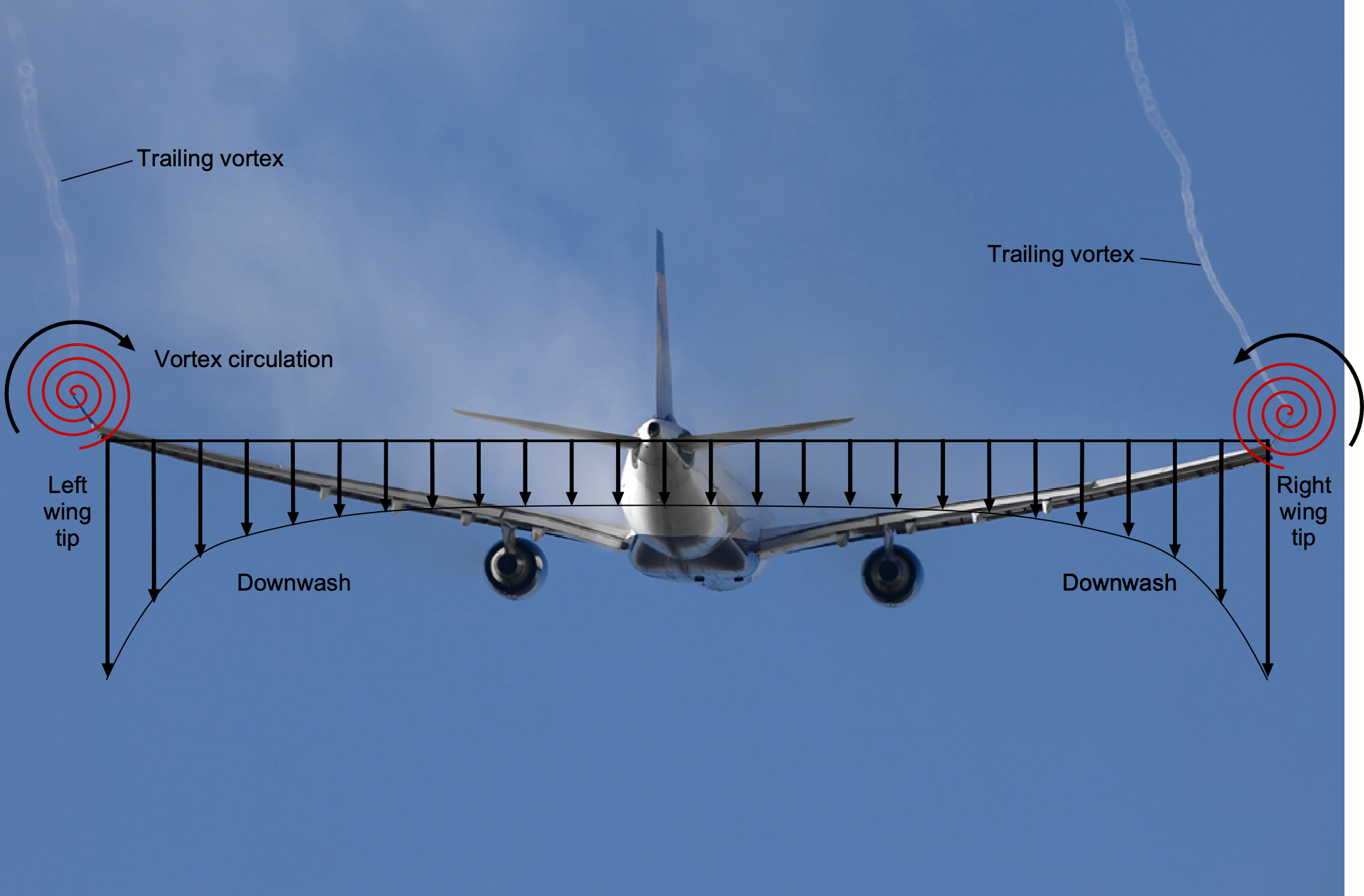
A wing’s aerodynamic performance, including its lift and drag characteristics, is significantly influenced by its geometric design. Factors such as planform shape (chord distribution), span and aspect ratio, and spanwise twist are all essential in determining the wing’s aerodynamic efficiency. The wing design process must carefully balance these elements to optimize lift generation and minimize induced drag, among other factors, thereby achieving the wing’s best aerodynamic performance for the intended application.
Lifting line theory is another cornerstone of classical aerodynamics, explaining and predicting the aerodynamic behavior of finite wings at low speeds, i.e., without considering compressibility effects. Unlike the two-dimensional airfoil theory, which assumes infinite span and aspect ratio, the lifting line theory accounts for the three-dimensional effects of finite wings, including the formation of trailing vortices and the creation of induced drag. By modeling the wing as a bound vortex line with a spanwise variation in circulation, along with the associated effects of the trailed vortex wake, this theory provides a sound mathematical framework for determining the spanwise lift distribution, induced drag, and overall aerodynamic efficiency of a finite wing.
Learning Objectives
- Understand how trailing vortices generate downwash and affect the angle of attack of a wing.
- Mathematically predict how and why the lift varies along the span of a finite wing and its impact on total lift and induced drag.
- Appreciate why an elliptical lift distribution on a wing minimizes its induced drag.
- Determine the total lift and induced drag of a finite wing of arbitrary shape.
- Apply the lifting line solutions to non-eliptical solutions such as for a flying wing.
- Review the extension of lifting line theory to lifting surface theory.
History
Lifting line theory, initially developed by Ludwig Prandtl and his students in the early 1900s, revolutionized the understanding of finite wing aerodynamics, marking a significant milestone in aeronautical developments. Before Prandtl’s work, aerodynamic theories were primarily based on two-dimensional airfoil analysis, which assumed a wing of infinite span and ignored the effects of the wing tip vortices and the three-dimensional impact caused by the wake. The work of Frederick Lanchester on the roll-up of wingtip vortices, as illustrated in a figure from his book shown below, was influential in establishing the importance of adequately modeling finite wing aerodynamics. Furthermore, as aviation advanced, particularly during WWI, including the transition from biplanes to higher-performance monoplanes by the 1920s, the predictive limitations of existing aerodynamic theories quickly became evident. Designers needed a way to better predict and optimize the performance of monoplane wings with finite span, particularly in terms of their lift and drag, as well as other factors such as aeroelastic characteristics and stalling behavior.
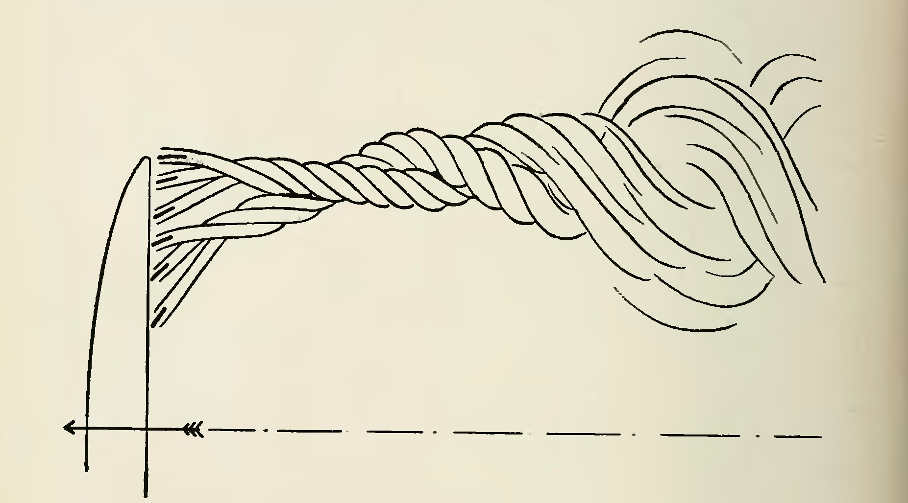
Prandtl’s lifting line theory[2] addressed this need by modeling a finite wing as a bound vortex line with a spanwise circulation distribution. Prandtl’s advance over Lanchester’s work was in the theoretical modeling of the wing, with its wake represented as a sheet of vortices trailing behind it. This wake produced a downwash flow, decreased the effective angle of attack along the entire wing and created induced drag, a drag component directly associated with lift production. Prandtl also demonstrated that an elliptical lift distribution over the wing span minimized the induced drag, setting a practical goal for efficient wing design. Prandtl’s original published works also show an “ideal” elliptical wing planform, which may have influenced the design of the Supermarine Spitfire in the early 1930s.
In the 1920s, Hermann Glauert[3] further refined and extended Prandtl’s work, making it more accessible and applicable to practical engineering problem-solving.[4] The use of straight vortex lines, as shown in the figure below from his book, allowed the induced velocity over the wing to be calculated using the Biot-Savart law, which formed the cornerstone of the lifting line theory. He then clarified the fundamental importance of the elliptical lift distribution and introduced systematic methods for analyzing wings of arbitrary planform and twist using a Fourier series, much like the approach employed in the thin airfoil theory.
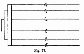
Glauert’s detailed methods for calculating induced drag helped bridge the gap between theoretical predictions and practical wing designs, making lifting line theory one of the first valuable approaches for three-dimensional wing analysis. Additionally, the theory was written in a form that later allowed it to be adapted to swept wings and non-planar configurations and extended to lifting surface methods that model the chordwise distribution of circulation. Though more advanced techniques, such as computational fluid dynamics (CFD), are now widely used, the lifting line theory remains a cornerstone of aerodynamic modeling. Its mathematical simplicity and elegance make it valuable for preliminary wing design and essential to aerodynamic education.
Helmholtz’s Vortex Theorems
Helmholtz’s vortex theorems describe the fundamental properties of vortex motion in an ideal fluid. First formulated by Hermann von Helmholtz in 1858, they remain central to understanding vorticity dynamics in fluid mechanics and aerodynamics. These theorems are derived from the Euler equations and express how vortex lines behave in an ideal flow.
- First Helmholtz Theorem (Conservation of Circulation): The circulation around a material loop moving with the fluid remains constant over time, i.e.,
 , where
  is the circulation. This theorem implies that vortices cannot spontaneously appear or vanish in an inviscid fluid. Circulation can only be introduced through boundaries or viscous effects, which are excluded in the ideal model. This result is consistent with Kelvin’s Circulation Theorem, which forms the foundation for Helmholtz’s first theorem. While Kelvin’s theorem asserts the conservation of circulation around any material loop in an ideal fluid, Helmholtz’s first theorem applies this principle specifically to vortex tubes, emphasizing that their circulation (vortex strength) remains constant along their length as the flow convects them.
 - Second Helmholtz Theorem (Conservation of Vortex Lines): Vortex lines move with the fluid. If a vortex line passes through a fluid element at some initial time, it will continue to pass through that fluid element at all later times. This implies that vortex lines are “frozen” into the fluid, i.e., the topology of the vortex structure is conserved as it is convected with the flow.
- Third Helmholtz Theorem (Strength of Vortex Tubes): The strength of a vortex tube (the circulation around any closed loop within the tube) is constant along its length and does not vary with time. This theorem follows from the divergence-free nature of the vorticity field in an ideal flow, i.e.,
 , which implies that vortex tubes cannot begin or end in the fluid interior, i.e., they must either form closed loops or terminate at boundaries.
Helmholtz’s theorems are foundational in studying vortex dynamics, including the formation and evolution of wingtip vortices and the inviscid modeling of aerodynamic flows. They are essential in developing the Biot-Savart law, the lifting-line theory, and other potential flow models that underpin much of classical aerodynamics. While real fluids are viscous and may violate these theorems under certain conditions, Helmholtz’s laws provide an essential idealized framework for understanding the behavior of vortex flows.
Theory of Vortex Lines
The line vortex is a fundamental singularity in fluid dynamics used to model velocity fields induced by a circulation, . The ideas of circulation and the effects associated with vortices have been previously introduced. A vortex line is a curve of any shape and tangent to the vortex, as shown in the figure below. Notice that a line vortex in three dimensions is analogous to a point vortex in two dimensions, but instead of being a singular point, it extends along a curve. The circulation around any closed curve is equal to the sum of the strengths of the line vortices intersecting the surface bounded by the curve. Consequently, a line vortex cannot terminate within a fluid. It must form a closed loop, end at a solid boundary, or extend to infinity, the principles formally embodied in Helmholtz’s theorems.

The Biot-Savart law describes the velocity field induced by such a circulation distribution, . Regarding the situation shown in the figure above, the increment in the downwash,  , from the vortex element
  can be mathematically expressed as
(1) 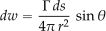
where is the circulation or vortex strength, is a differential element of the line vortex,  is the distance of the point P from the element, and
  is the angle between the direction of the element and the straight line joining the element to the point P. Notice that the element of a line vortex cannot exist by itself and only forms the basis for integrating the effects along a line vortex of finite length.
Straight Line Vortices
Straight-line vortices are used in the development of the finite-wing theory. Consider the evaluation of the induced velocity of a straight-line vortex of finite length AB, as shown in the figure below. If PN has a perpendicular length  , then the induced velocity at P from the element at point Q is
(2) 
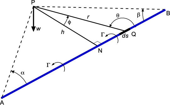
To show this result, the element may be geometrically expressed as
(3) 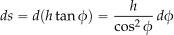
where the angle  is as shown in the figure above, so that
(4) 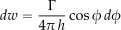
The total induced velocity is then obtained by integration along the length of the vortex line using
(5) 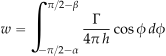
which gives
(6) 
Doubly-Infinite Straight Line Vortex
If, as a special case, the line is of doubly infinite length, as shown in the figure below, then it will be apparent that  , so the general result reduces to
(7) 
which is consistent with the result of a two-dimensional point vortex.
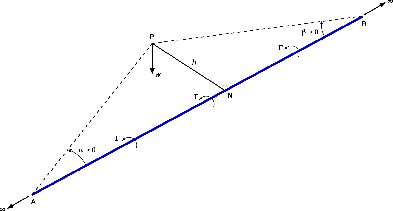
Singly-Infinite Straight Line Vortex
For a singly infinite vortex, which starts at point N and then extends to infinity only in one direction, as shown in the figure below, then  and
and  , and the downwash is given by
(8) 
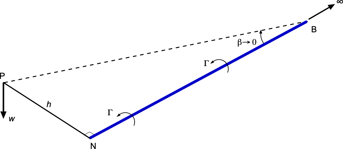
This latter result for the downwash from a semi-infinite line vortex is extensively used in developing the lifting line theory, in which several line vortices are combined appropriately to represent the physics of the flow produced by a finite wing.
Lifting Line Theory
The following exposition of the lifting line theory and the development of the monoplane wing equation follows the work of Gluert. In addressing the problem of a wing of finite span in three-dimensional flow, the following assumptions were made:
- The wing’s chord is relatively minor compared to its span, resulting in a high aspect ratio.
- The wing’s spanwise axis can be considered a straight line perpendicular to the freestream flow, i.e., the wing is unswept.
- The wing planform is symmetrical laterally about its centerline, i.e., the left and right wing panels mirror each other.
Apart from these restrictions, the planform (chord), pitch angle (including any twist angle), and zero-lift angle of the airfoil section may vary arbitrarily across the wing’s span.
Bound & Trailed Vortices
If a wing generates lift, there must be a flow circulation around each airfoil section comprising the wing, effectively creating a line vortex or a set of line vortices along the wing’s span. These line vortices, which are attached to the wing, as shown in the figure below, are referred to as the bound vortices and create lift in accordance with the Kutta-Joukowsky theorem. Physically, these bound vortices are formed by the integrated effect of the vorticity in the boundary layer or equivalent vortex sheet surrounding the airfoil’s surface, as in the manner used to develop the thin airfoil theory. According to the general theory of vortex flows and Helmholtz’s theorems, these bound vortices cannot terminate at the tips of the wing but must extend off the wing tips into the fluid as free line vortices. These are referred to as the trailing or trailed vortices, as illustrated in the figure below.
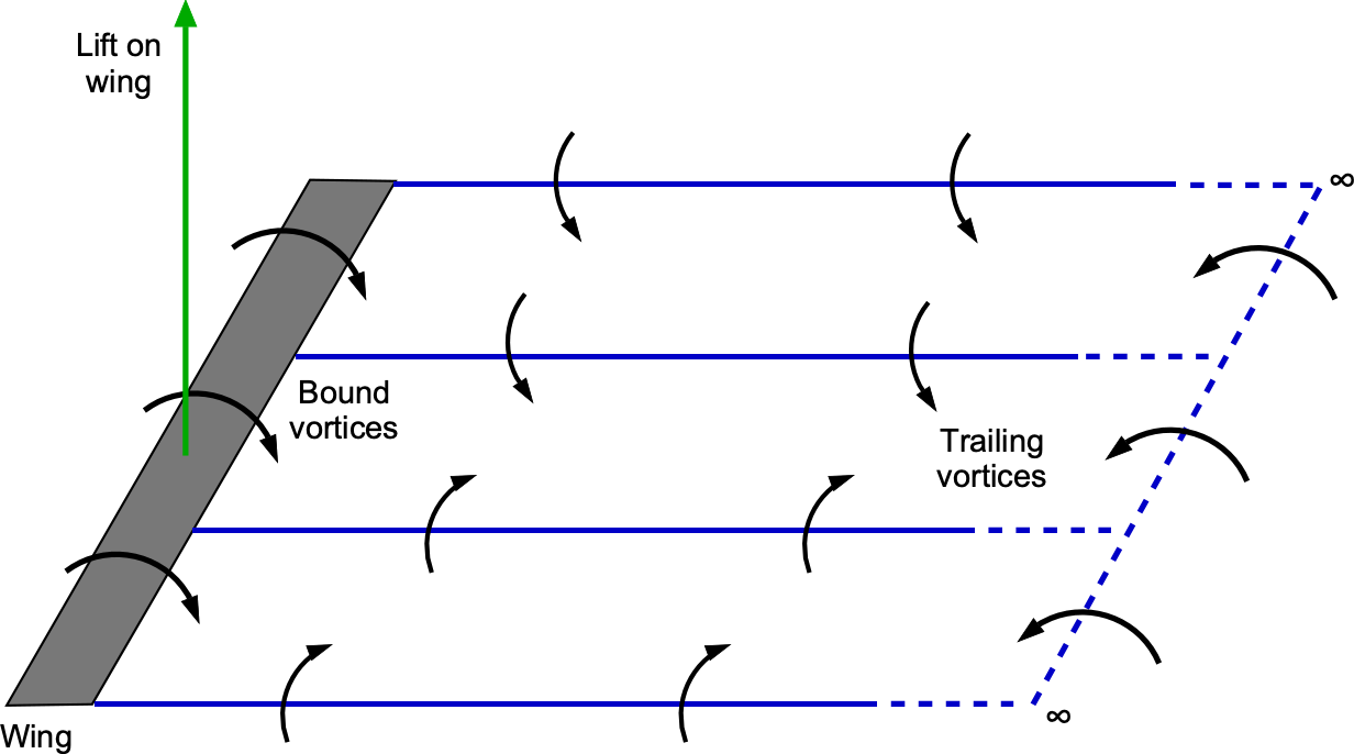
This entire vortex system, which extends to infinity far behind the wing, is completed by a transverse vortex parallel to the span. However, this vortex has no consequence in the steady state as its induced effects are asymptotically zero. For practical purposes, the trailing vortices can be considered to align with the freestream flow and extend downstream to infinity as a singly infinite line vortex.
Horseshoe Vortex System
Glauert describes the simplest type of vortex system as occurring when the circulation around each airfoil section has a constant value across the wing’s span. The bound vortex system can then be represented as a single “lumped” line vortex with strength , which, to be consistent with the thin airfoil theory, can be positioned at the aerodynamic center along the 1/4-chord of the wing, as shown in the figure below. The trailing vortices will consist of two line vortices, each with the same strength, originating from the tips of the wing and extending downstream in the direction of the freestream flow. This representation is called a “horseshoe vortex system.”
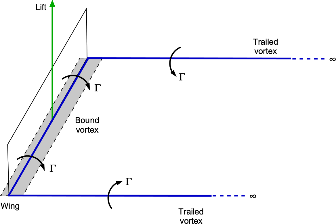
In practice, the vortices trailing from the wing tips will generally not be straight lines because of variations of the downwash at different distances behind the wing. Experiments show that as they develop downstream, the trailing vortices tend to descend below the wing and contract inward. However, as Glauert explains, they can be approximated as straight lines parallel to the direction of motion for most practical purposes. This assumption leads to the simplified representation of the wing and its wake as a horseshoe vortex system, which forms the fundamental basis of the lifting line theory.
Nested Horseshoe System
In reality, the vortex system of an aerofoil is more complex because the circulation is not uniform across the span. Instead, it typically reaches its maximum value at the center and tapers to zero at the tips. This distribution can be represented by superimposing multiple simple “horseshoe vortex systems,” as shown in the figure below. This setup yields a more accurate representation of the vortex system over the wing and in its wake.
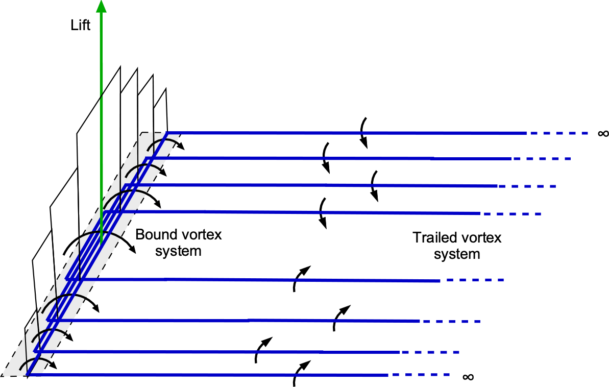
This model then comprises interlaced bound vortices, all colocated at the aerodynamic center on the 1/4-chord axis, and a sheet of trailing vortices extending from the wing’s trailing edge. Glauert used this representation of the vortex system as the fundamental premise in developing the mathematics of the lifting line model.
Wake Rollup
As Glauert explains, the origin of the trailing vortex wake system can also be understood from the perspective of the pressure difference between the upper and lower surfaces of the wing. Suppose the lift distribution across the span of a wing reaches a maximum at its centerline. In that case, there will be a significant decrease in pressure above the wing and an increase in pressure below it, as shown in the figure below. These pressure differences decrease towards the tips of the wing because of the influence of the trailing wing tip vortices.
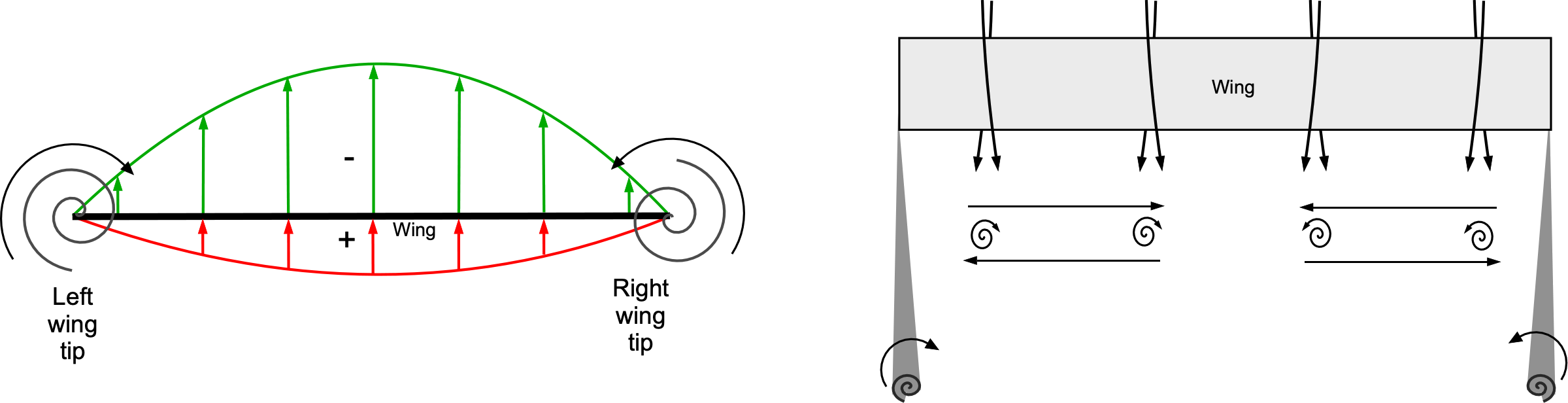
As the streamlines pass above the wing and flow inward toward the center, while those below the wing flow outward, they leave the trailing edge and form a discontinuity surface, as shown in the figure above. The trailing vortices from the wing then represent the vorticity of this discontinuity surface. The sheet of trailing vortices rolls up into a pair of concentrated vortices downstream, forming the characteristic pair of vortices behind a wing, as observed in practice using flow visualization methods.
Nearer to the wing, the influence of the trailing vortex system can be modeled by assuming that the individual trailing vortices extend downstream as straight lines. For the wake farther from the wing, which tends to contract somewhat, it is perhaps more accurate to assume a horseshoe vortex system with a span a little shorter than the wing span. Both representations are sufficiently representative of the actual flow physics for modeling purposes.
Calculating the Induced Velocity
In general, the circulation  will vary across the span of a wing, being symmetrical about the centerline and decreasing to zero at the tips. Consistent with the nested horseshoe vortex model, between the points
  and
and  of the span of the wing, the circulation can be assumed to decrease by an amount
(9) 
Therefore, a trailed wake filament of this strength originates from the element  of the span, as shown in the figure below.
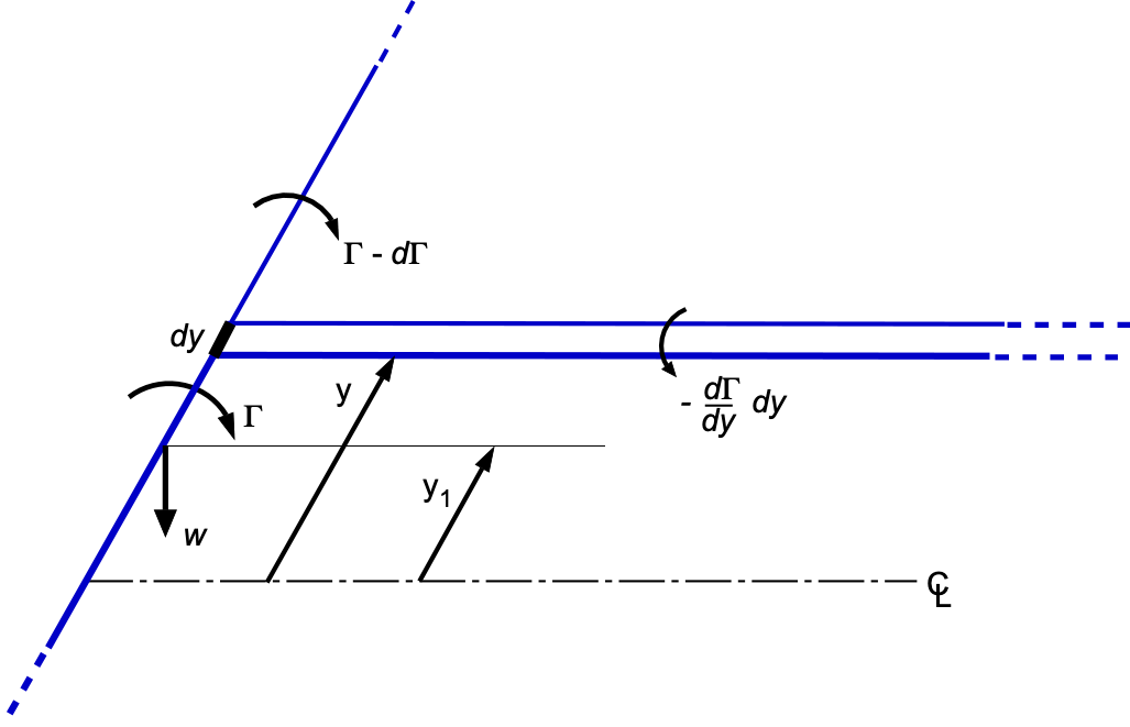
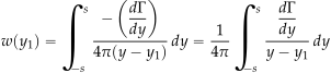
Therefore, in the aggregate, a sheet of trailing vortices will extend behind the entire wingspan because of the continuous change in along the wing, i.e., . The induced downwash at any point of the span will then be obtained as the sum of the effects of all the trailing vortices of this sheet. For example, consider some reference point on the wing, say  . Using Eq. 8, the downwash at this point from all of the trailing line vortices comprising the sheet will be
(10) 
This latter result will then apply at every section, , along the span of the wing, and different values of  will be obtained depending on the distribution, , and the proximity to the wing tips. It will be apparent from the previous discussion that the circulation gradient, i.e.,
  , is much higher at the wing tips, so the trailed wake will have a greater circulation here. This behavior is consistent with Lanchester’s interpretation of the wake generated behind a wing. The question now is how this downwash distribution can be calculated as it affects the lift and drag at each wing section, , and the overall wing lift and drag.
Sectional Effects of the Induced Velocity
The induced velocity from the trailed wake will affect the aerodynamic angle of attack at each section across the wing. Adding the downwash flow vector  to the freestream flow vector
  produces a resultant flow velocity (or local relative wind) that turns through an angle
  , called the induced angle of attack, as shown in the figure below. It will be apparent that the resultant flow now approaches the wing at a different angle, creating a reduced “effective” angle of attack,
  .
.
 is to cause a realignment of the relative wind to the wing section, effectively tilting the lift vector aft to produce a component of drag.
From the geometry, as shown above, the induced angle, , is given by
(11) 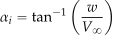
which will, in general, be different at each station on the wing, i.e.,  and
and  . For small angles, which is typical for a wing, it is sufficient to write that
(12) 
Therefore, the effective (and lower) angle of attack of the wing section is now
(13) 
This outcome means that the corresponding lift per unit span will be reduced from its two-dimensional value, i.e., the lift obtained without the effects of the downwash flow. Notice that because will typically be much smaller than , then the resultant velocity,  , can be assumed to be equal to , i.e.,
(14) 
It is particularly significant in this situation to note that the lift vector at each section assumes a new orientation and is tilted slightly rearward from its original direction in two-dimensional flow, thereby reducing the vertical component of the lift for a given angle of attack. The consequence is that there is now a component of the lift that acts in the downstream direction, which explains the origin of the induced drag,  , i.e.,
(15) 
Development of the Monoplane Wing Equation
With an understanding of the aerodynamic elements that comprise the problem of modeling a finite wing, the development of the fundamental equation of lifting line theory can be established, known as the monoplane wing equation.
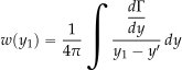
Connection Between Circulation and Downwash
As previously shown, if is the circulation produced around any section of the wing, the downwash from the trailing wake system at a point of the span is determined using
(16) 
A representative wing section, therefore, experiences the lift force corresponding to the two-dimensional conditions at the effective angle of attack, i.e.,
(17) 
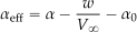
If the angles of attack  and are measured from the angle of zero lift of the airfoil section,
 , then
(18) 
Therefore, the lift coefficient of the wing section will be
(19) 
where  is the slope of the curve of lift coefficient against the angle of attack for the wing section in two-dimensional flow.
Furthermore, the circulation around the wing section can be connected to the lift coefficient,  , using
(20) 
This means that
(21) 
Therefore, it is possible to determine the circulation and the downwash for any wing in terms of the chord and angle of attack of the wing sections, which may vary across its span.
When the circulation and the downwash of any monoplane wing have been determined, the lift and induced drag are obtained by evaluating the integrals
(22) 
Use of the sectional lift curve slope
Strictly, the lift curve slope, , for which Glauert assigns the symbol  , depends on the shape(s) of the wing section(s). However, two-dimensional thin airfoil theory has shown that
  per radian angle of attack. It is known from experiments that is approximately equal to
  for all practical wing sections at low Mach numbers, and hence any normal variations in may be neglected without any appreciable loss of accuracy. Nevertheless, because a wing section may differ from the theoretical value
  , it is best to retain the value of as a variable, and the theoretical value of is generally only used only in theoretical solutions.
Method of Solution
Glauert used a transformation[5] to replace the coordinate , measured to the left wing tip along the span of the wing from its center, by the angle , as defined by
(23) 
where  is the semi-span. It will be apparent that as varies from
  to
to  , then varies from
  to
to  across the span from the left tip to the right. The circulation, , which is a function of , can then be expressed as the Fourier series
(24) 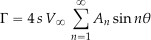
where the values of the coefficients  must be determined by connecting the distribution of “bound” to the wing with
  produced by the trailed wake in a consistent manner.
Notice that the series chosen for the circulation satisfies the condition that the circulation decreases to zero at the wing tips. As shown in the figure below, if the wing is flying in level flight, then the spanwise loading will be symmetrical about its centerline, and only odd integral values of  will occur in the Fourier series.
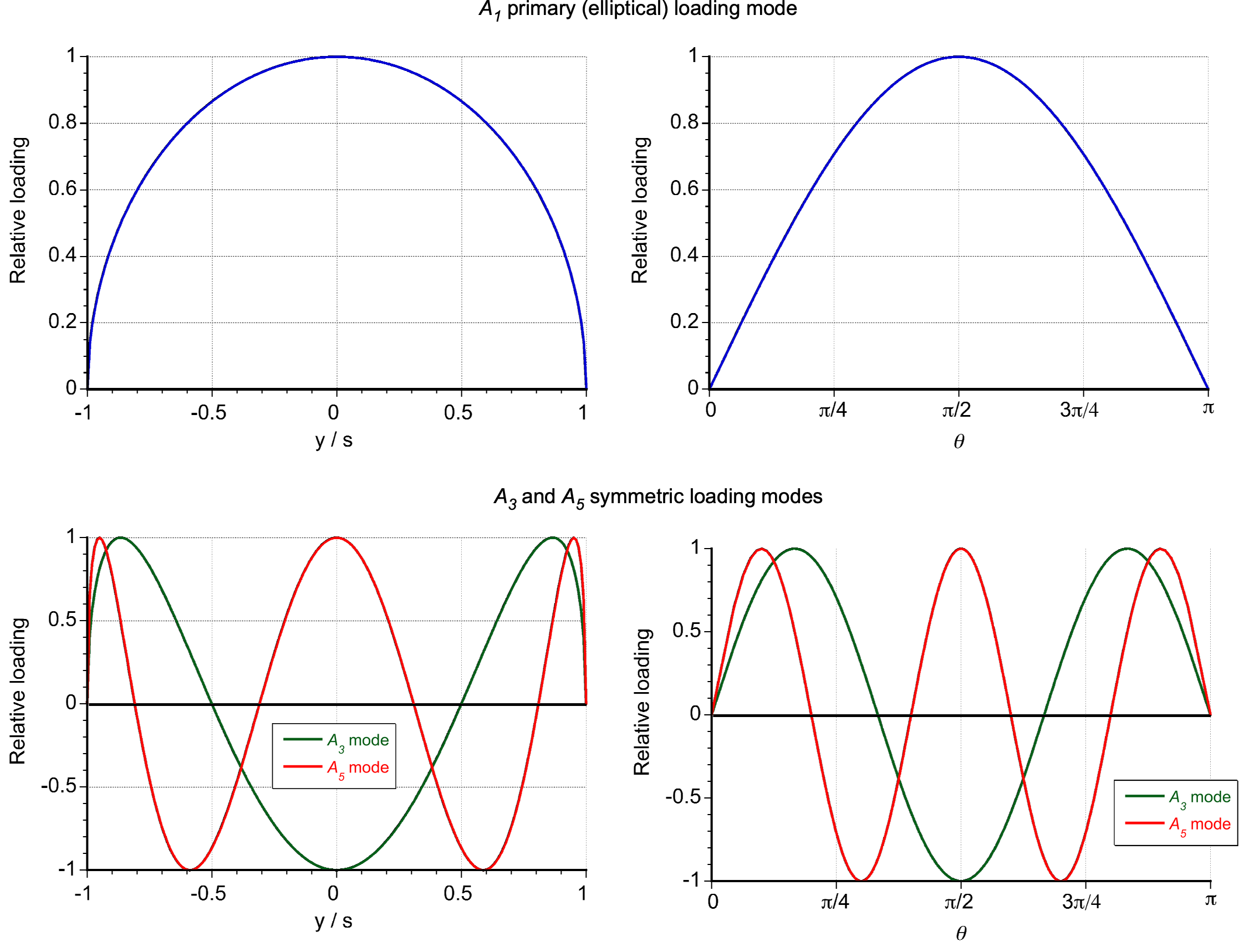
It will be apparent that the primary mode is the  or
or  mode, corresponding to an elliptical circulation distribution over the wing. Because
  , then
(25) 
Simplifying gives
(26) 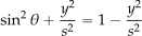
and so
(27) 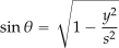
which is elliptical. The higher symmetric modes, i.e.,  , for which
  and
and  are shown in the figure below, represent a symmetric modification to the primary loading, i.e., a deviation from the elliptically distributed form.
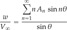
The downwash at the point or  of the wing now becomes
(28) 
because
(29) 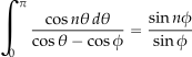
Therefore, at the general point of the wing, the downwash is
(30) 
Monoplane Wing Equation
The equation connecting the circulation and the downwash velocity now becomes
(31) 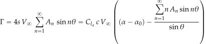
which gives
(32) 
(33) 
Equation 33 is called the fundamental equation of lifting line theory or the monoplane wing equation and can be used to determine the coefficients values for any monoplane[6] wing. It is generally solved numerically. The equation must be satisfied at all points of the wing, but because the wing is symmetrical about its mid-point in level flight, it is usually sufficient to consider values of between and  . In this case, only the symmetric modes, i.e., , must be evaluated. The dimensionless Glauert parameter
  , which is proportional to the chord
  , and the angle of attack , will generally depend on wing twist, e.g., if the wing has wash-out.
Lift and Induced Drag
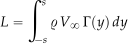
The lift on the wing is given by
(34) 
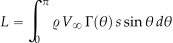
Switching to the spanwise angle coordinate, , where  and
and  , the lift becomes
(35) 
Substituting the general series expression for circulation gives
(36) 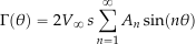
and so
(37) 
Using the orthogonality property of sine functions, i.e.,
(38) ![\begin{equation*} \bigintsss_0^\pi \sin(n\theta) \, \sin(\theta) \, d\theta = \begin{cases} \dfrac{\pi}{2}, & n = 1 \\[12pt] 0, & n \neq 1 \end{cases} \end{equation*}](https://eaglepubs.erau.edu/app/uploads/quicklatex/quicklatex.com-6cc8846088a0343747caf08b0a219ebe_l3.svg "Rendered by QuickLaTeX.com")
then the only term that contributes to the integral is , so
(39) 
The coefficient,  , which is the elliptical loading mode, is related to the lift coefficient,
  , using
(40) 
The induced drag is determined using
(41) 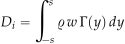
Switching to the coordinate gives
(42) 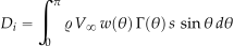
Recall that the downwash velocity is given by
(43) 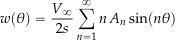
Substituting  and
and  gives
gives
(44) 
Expanding the summation gives
(45) 
Again, the orthogonality of  functions ensures that only terms where
  are retained, so that
(46) 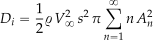
It is convenient to write
(47) 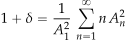
so the induced drag,  , is
, is
(48) 
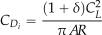
In terms of drag coefficient, then
(49) 
The total drag coefficient includes both profile drag and induced drag. If the profile drag coefficient  varies across the span, the profile drag coefficient for the wing is
(50) 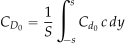
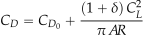
Adding the induced drag gives
(51) 
Asymmetric Loading Modes
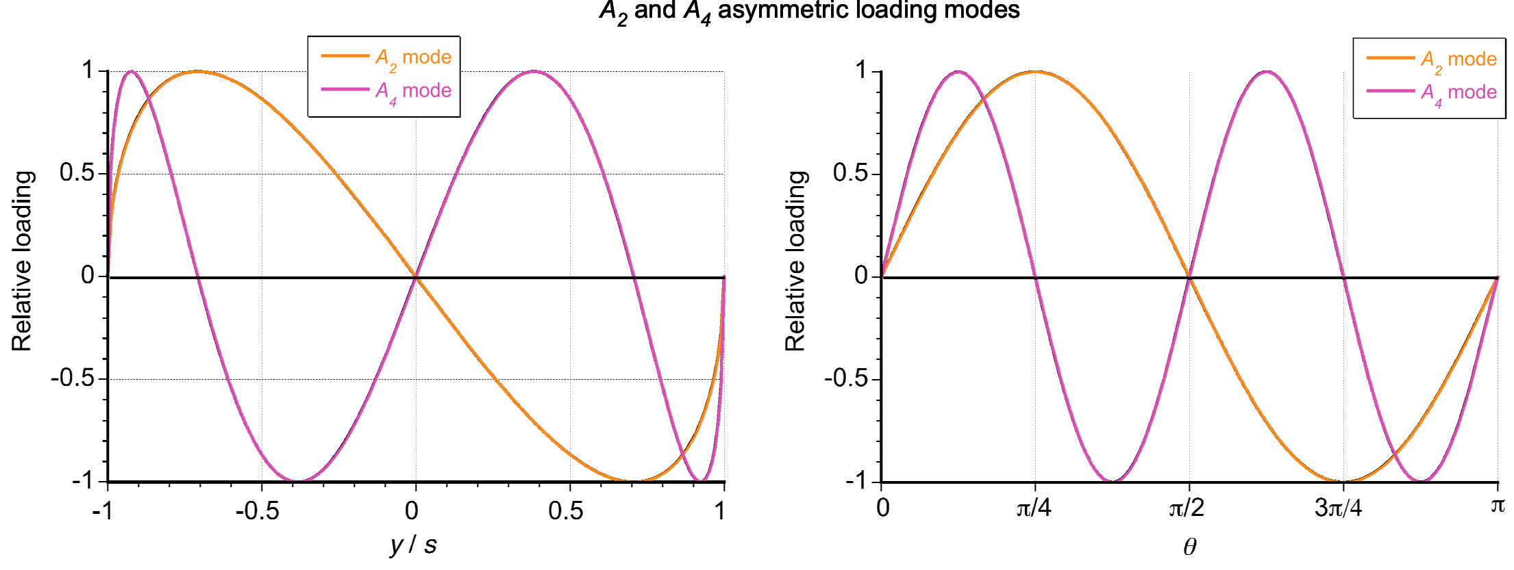
The even modes in the lifting line theory represent an asymmetric lift distribution. These modes can arise from aileron deflections and angular velocity of the wing in roll, yaw, sideslip, or other asymmetries along the wing’s span. This situation then leads to lift asymmetry, influencing rolling moments, possible yawing moments, and induced drag. For example, ailerons are control surfaces located near the wingtips, which are deflected asymmetrically to induce a rolling moment about the aircraft’s longitudinal axis. The figure below shows that their operation produces asymmetric modes in the lifting-line theory, particularly  and other higher even-numbered modes.
The total circulation distribution can be expressed as
(52) 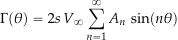
where represents the symmetric lift distribution from the freestream velocity, and captures the antisymmetric lift contribution from aileron deflection, as shown in the figure below. The primary contribution from the ailerons is
(53) 
The coefficient depends on the aileron deflection angle  , which modifies the local angle of attack near the wingtips, i.e.,
(54) 
where  is the aspect ratio. The constant of proportionality depends on the actual wing’s geometry and aerodynamic characteristics. For small deflection angles, is approximately linear in .
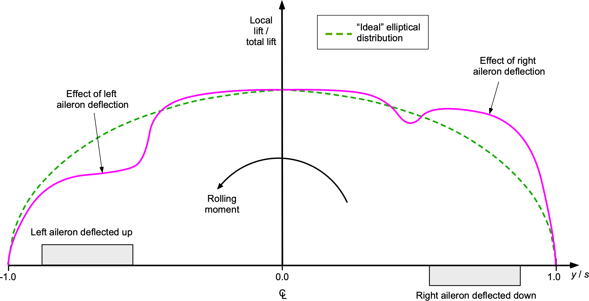
The resulting rolling moment,  , about the longitudinal axis, is directly related to this antisymmetric lift distribution, i.e.,
(55) 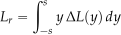
where  is the lift difference from aileron deflection at spanwise location . This rolling moment scales with , i.e.,
(56) 
From a design perspective, proper sizing and placement of ailerons are crucial to ensure sufficient rolling authority without excessive induced drag or adverse yaw effects. To this end, the lifting line theory can provide valuable insight into the aileron designs that may be required.
Worked Example #1 – Further understanding of circulation modes
An untwisted elliptical wing planform is installed symmetrically in a wind tunnel with its centerline along the tunnel axis. If the air in the wind tunnel has a freestream axial velocity and also has a small angular velocity  about the tunnel axis, show that there will be an extra asymmetric distribution of circulation along the wing given by
![\[ \Gamma = 4 s \, A_2 \, \sin(2\theta) \]](https://eaglepubs.erau.edu/app/uploads/quicklatex/quicklatex.com-a418dfb03a0ad1f3c3c7b01b1f36cea8_l3.svg "Rendered by QuickLaTeX.com")
Determine in terms of and the wing parameters.
Show solution/hide solution.
From the lifting-line theory, the spanwise circulation distribution can be expressed as a Fourier sine series, i.e.,
![\[ \Gamma(\theta) = 2s \, V_{\infty} \sum_{n=1}^\infty A_n \, \sin(n\theta) \]](https://eaglepubs.erau.edu/app/uploads/quicklatex/quicklatex.com-f97c2d6117a005a02a2045dc9e7708f7_l3.svg "Rendered by QuickLaTeX.com")
where is the semi-span of the wing, is the spanwise angular coordinate related to the spanwise position by  , and are the Fourier coefficients determined by the flow and wing properties. For an elliptic wing, the baseline lift distribution from the freestream flow, , corresponds to the
  term and perturbations introduced by that will manifest as higher harmonics, starting with
  .The angular velocity induces a spanwise velocity component
  at a location , given by
![\[ v_y = \omega \, y = \omega \, s \, \cos\theta \]](https://eaglepubs.erau.edu/app/uploads/quicklatex/quicklatex.com-11d96dc627f7cee694e37b09e8aa4177_l3.svg "Rendered by QuickLaTeX.com")
This spanwise velocity modifies the local effective angle of attack  , and the change in angle of attack
  is
is
![\[ \Delta\alpha(y) = \frac{v_y}{V_{\infty}} = \frac{\omega y}{V_{\infty}} = \frac{\omega s \cos\theta}{V_{\infty}} \]](https://eaglepubs.erau.edu/app/uploads/quicklatex/quicklatex.com-ddbf11495e77ad84b53e9f992d7b1b2c_l3.svg "Rendered by QuickLaTeX.com")
Therefore, the angular velocity introduces a spanwise perturbation in  , which varies linearly with
  . The local circulation (y) or is proportional to the effective angle of attack , so the perturbation in circulation
  from will be
![\[ \Delta\Gamma(y) \, \propto \, \Delta\alpha(y) \]](https://eaglepubs.erau.edu/app/uploads/quicklatex/quicklatex.com-25c67efdbc8d0c8ee8087eba2e63e575_l3.svg "Rendered by QuickLaTeX.com")
Substituting 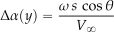 gives
gives
![\[ \Delta\Gamma(y) \, \propto \, \frac{\omega \, s \, \cos\theta}{V_{\infty}} \]](https://eaglepubs.erau.edu/app/uploads/quicklatex/quicklatex.com-a700ffa46aa9da76efd330168dfe99f3_l3.svg "Rendered by QuickLaTeX.com")
For an elliptical wing, the spanwise variation contributes to the  term in the series expansion. This means that
![\[ \Delta\Gamma(\theta) = 4s \, A_2 \, \sin(2\theta) \]](https://eaglepubs.erau.edu/app/uploads/quicklatex/quicklatex.com-b68868de4c4aa8809455b7d7077599a3_l3.svg "Rendered by QuickLaTeX.com")
where is the second harmonic, specifically
![\[ A_2 \, \propto \, \frac{\Delta\alpha(y)}{C_{l_{\alpha}}} \]](https://eaglepubs.erau.edu/app/uploads/quicklatex/quicklatex.com-eec840d5de459a483a79a760c4584aa3_l3.svg "Rendered by QuickLaTeX.com")
where is the lift curve slope (per radian). Substituting 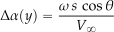 , then
![\[ A_2 = \frac{\omega s}{4 V_{\infty}} \]](https://eaglepubs.erau.edu/app/uploads/quicklatex/quicklatex.com-64295ca6001354f5e270d448ff9e3875_l3.svg "Rendered by QuickLaTeX.com")
Elliptic Spanwise Loading
The lift and induced drag of a wing are given by
(57) 
For a wing of a given size, the coefficient has a fixed value independent of the wing’s shape. The induced drag will be minimized when all higher-order coefficients ( ) in the series for circulation are zero, i.e.,
  . In this case, the distribution of circulation across the span of the wing simplifies to
(58) 
so the circulation is elliptically loaded. Putting  into Eq. 33 gives
(59) 
and so
(60) 
The corresponding induced drag coefficient will be
(61) 
Notice that the result of the downwash becomes
(62) 
and the equivalent angle of attack is
(63) 
along the span. This result implies that the local lift coefficient, , is constant across the span, as shown in the figure below.
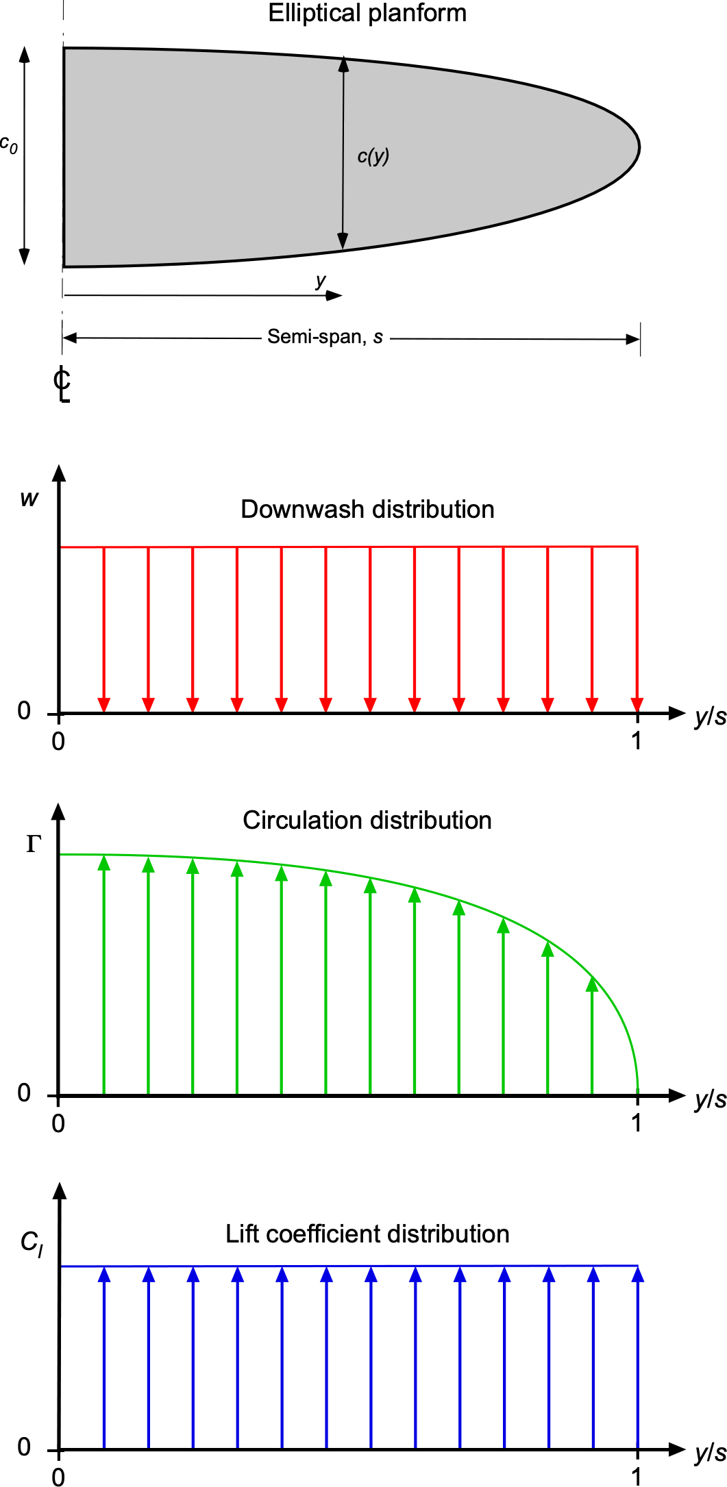
To produce a constant and an elliptic circulation distribution, the chord length must vary elliptically along the span. This result can be obtained by using
(64) 
where it will be apparent that
(65) 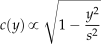
so that a solution is
(66) 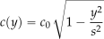
where  is the chord length at the wing root. This special case of elliptic loading is significant for several reasons:
- It results in the minimum possible induced drag for a given total lift, i.e., .
- Most conventional wing designs closely approximate an elliptic load distribution, making it a valid first-order approximation.
- The results derived from the assumption of elliptic loading represent the optimal scale for minimizing induced drag while remaining applicable to practical wing designs.
- Elliptic loading (or almost elliptic) can also be achieved with wings of non-elliptic planforms by suitably varying the twist angle along the span.
Effect of Aspect Ratio
The results developed for the lift and drag coefficients of an elliptic wing can be used to calculate the effect of a change in aspect ratio. If the aspect ratio is reduced from to  , the changes in the drag coefficient at a given value of the lift coefficient is
(67) 
It will be apparent that wings with a higher aspect ratio have aerodynamic advantages, all other factors being equal, e.g., wing area and planform shape.
While this formula for the drag coefficient applies only to wings with an elliptical loading, the lift distribution curves for rectangular and most airplane wings do not differ significantly from the elliptic form. Therefore, the formula may be used more generally to calculate the effect of a modest aspect ratio change.
Effect on Lift Curve Slope
The assumptions are: 1. The two-dimensional lift curve slope for the airfoil is  , which assumes no three-dimensional effects. 2. The lift curve slope for the finite wing is , which includes the effects of finite aspect ratio (
 ). The lifting line theory introduces an induced angle of attack caused by the downwash from the wing’s trailing vortices. The net angle of attack,
  , is related to the effective angle of attack,
  , and the induced angle, , by
(68) 
The total lift coefficient is then
(69) 
where the two-dimensional lift curve slope has been replaced with using Gluert’s notation. The induced angle of attack is related to the lift coefficient and aspect ratio
(70) 
Substituting this back into the lift equation gives
(71) 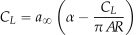
and rearranging gives
(72) 
Dividing through by gives
(73) 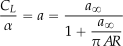
Therefore, for wings with a high aspect ratio or a small , the lift curve slope approaches the two-dimensional value, corrected by an aspect ratio term to account for three-dimensional effects.
Worked Example #2 – Aerodynamic characteristics of an elliptical wing
An elliptical wing has the following characteristics:
- Span,
 = 10 m.
 - Planform area,
 = 8 m
= 8 m .
. - Angle of attack, = 5
 .
. - Zero-lift angle of attack, = -0.5.
- 2-dimensional lift curve slope, = = 2 per radian.
Compute:
1. The wing’s lift coefficient, .
2. The corresponding induced drag coefficient,  .
.
Show solution/hide solution.
The aspect ratio of the wing is
![\[ A\!R = \dfrac{b^2}{S} = \dfrac{10^2}{8} = 12.5 \]](https://eaglepubs.erau.edu/app/uploads/quicklatex/quicklatex.com-f6fb525124d1d5c4940142217cf876c2_l3.svg "Rendered by QuickLaTeX.com")
The lift curve slope of the wing adjusted for 3-dimensional effects is
![\[ a = \dfrac{a_{\infty}}{1 + \dfrac{a_{\infty}}{\pi \, A\!R}} = \dfrac{2\pi}{1 + \dfrac{2\pi}{\pi \times 12.5}} = 5.418 \]](https://eaglepubs.erau.edu/app/uploads/quicklatex/quicklatex.com-7dddd4ab555deace4f5109d8c83f5bdf_l3.svg "Rendered by QuickLaTeX.com")
The lift coefficient is
![\[ C_L = a (\alpha - \alpha_0) = 5.418 \left(\dfrac{5\pi}{180} - \dfrac{-0.5\pi}{180}\right) = 0.520 \]](https://eaglepubs.erau.edu/app/uploads/quicklatex/quicklatex.com-23560ab6f9df89bba94201409c057b0a_l3.svg "Rendered by QuickLaTeX.com")
For an elliptical wing, the induced drag coefficient is
![\[ C_{D_i} = \dfrac{C_L^2}{\pi \, A\!R} = \dfrac{(0.520)^2}{\pi \times 12.5 \times 1} = 0.00688 \]](https://eaglepubs.erau.edu/app/uploads/quicklatex/quicklatex.com-f2856aaf82b7ef418fa1ad7eb48403e9_l3.svg "Rendered by QuickLaTeX.com")
Numerical Solution to the Monoplane Wing Equation
The governing equation for the monoplane wing is
(74) 
where:
- are the coefficients of the circulation expansion.
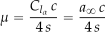 is referred to as Glauert’s non-dimensional parameter.
- is the geometric angle of attack, or more correctly, pitch angle.
- is the chord length (may vary with
 and so ).
 - is the semi-span of the wing.
To solve numerically, the domain ![\theta \in [0, \pi]](https://eaglepubs.erau.edu/app/uploads/quicklatex/quicklatex.com-a4b289d6310ea443777e61ec16fbc147_l3.svg "Rendered by QuickLaTeX.com") is divided into
is divided into  discrete points, i.e.,
(75) 
At each discrete point  , the governing equation becomes
(76) 
This equation can be rewritten in matrix form as
(77) 
where ![\mathbf{A} = [A_1, A_2, \cdots, A_N]^T](https://eaglepubs.erau.edu/app/uploads/quicklatex/quicklatex.com-3468ab6636bd83a959febb3d4da5babd_l3.svg "Rendered by QuickLaTeX.com") is the vector of unknown coefficients;
is the vector of unknown coefficients; ![\mathbf{b} = [b_1, b_2, \cdots, b_N]^T](https://eaglepubs.erau.edu/app/uploads/quicklatex/quicklatex.com-6f0898085b57c6d81c4f008962612ac1_l3.svg "Rendered by QuickLaTeX.com") is the right-hand side vector containing the the wing properties;
is the right-hand side vector containing the the wing properties;  is the influence coefficient matrix.
The components of the matrix equation are
(78) 
and
(79) 
The matrix equation is expanded as
(80) ![\begin{equation*} \begin{bmatrix} M_{11} & M_{12} & \cdots & M_{1N} \\[8pt] M_{21} & M_{22} & \cdots & M_{2N} \\[8pt] \vdots & \vdots & \ddots & \vdots \\[8pt] M_{N1} & M_{N2} & \cdots & M_{NN} \end{bmatrix} \begin{bmatrix} A_1 \\[8pt] A_2 \\[8pt] \vdots \\[8pt] A_N \end{bmatrix} = \begin{bmatrix} b_1 \\[8pt] b_2 \\[8pt] \vdots \\[8pt] b_N \end{bmatrix} \end{equation*}](https://eaglepubs.erau.edu/app/uploads/quicklatex/quicklatex.com-ddc8796696f404130669acac90197273_l3.svg "Rendered by QuickLaTeX.com")
where  and
and 
The unknown coefficients are found by solving
(81) 
Efficient numerical methods, such as LU decomposition, are typically used for inverting when is large.
Once the coefficients  are determined, the following aerodynamic quantities can be computed:
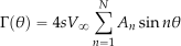
- The spanwise circulation distribution, , i.e.,
(82)
- The lift distribution,
 , and the lift coefficient, . The total lift coefficient is directly related to , i.e.,
(83)

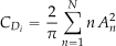
- The induced drag coefficient, which is computed using
(84)
Worked Example #3 – Numerical solution of the monoplane wing equation
A rectangular wing has the following geometric and operating conditions:
- Span,
 = 10 m.
 - Chord, = 1.0 m.
- Angle of attack, = 12.
- Zero-lift angle of attack, = -0.5.
- Lift curve slope,
 = 2 per radian.
 - Free-stream velocity,
 = 50 m/s.
 - Air density,
 = 1.225 kg/m
 .
.
Set up a numerical solution of the monoplane wing equation to determine:
1. The spanwise circulation distribution, .
2. The lift coefficient, .
3. The induced drag coefficient, .
Use five spanwise modes to approximate your answer.
Show solution/hide solution.
The semi-span is
![\[ s = \frac{b}{2} = \frac{10}{2} = 5 \, \text{m} \]](https://eaglepubs.erau.edu/app/uploads/quicklatex/quicklatex.com-ff0d0afabe7f22c28e1524a770af9b81_l3.svg "Rendered by QuickLaTeX.com")
so the non-dimensional parameter is
![\[ \mu = \frac{C_{l_\alpha} c}{4s} = \frac{2\pi \times 1.0}{4 \times 5} = 0.3142 \]](https://eaglepubs.erau.edu/app/uploads/quicklatex/quicklatex.com-6002d0c99ecf111cff11aba7070d1571_l3.svg "Rendered by QuickLaTeX.com")
The geometric angle of attack (allowing for the zero-lift angle) is
![\[ \alpha_{\text{geom}} = \alpha - \alpha_0 = 12^\circ - (-0.5^\circ) = 12.5^\circ = \frac{12.5\pi}{180} = 0.2182 \, \text{radians} \]](https://eaglepubs.erau.edu/app/uploads/quicklatex/quicklatex.com-2785373aa9072f398fc9ef2703726001_l3.svg "Rendered by QuickLaTeX.com")
Dscretize into  into equally spaced angular points, i.e.,
![\[ \theta_i = \frac{i \, \pi}{N-1}, \quad i = 0, 1, 2, 3, 4 \]](https://eaglepubs.erau.edu/app/uploads/quicklatex/quicklatex.com-0b3a1517e86c8f4f53080496915d3625_l3.svg "Rendered by QuickLaTeX.com")
Therefore,
![\[ \theta_0 = 0, \, \theta_1 = \frac{\pi}{4}, \, \theta_2 = \frac{\pi}{2}, \, \theta_3 = \frac{3\pi}{4}, \, \theta_4 = \pi \]](https://eaglepubs.erau.edu/app/uploads/quicklatex/quicklatex.com-341eff6a87e7c05cd66cc2b587ab75cd_l3.svg "Rendered by QuickLaTeX.com")
The governing equation with odd Fourier coefficients is
![\[ \sum_{n=1, 3, 5, 7, 9} A_n \, \sin n\theta_i \left( n \, \mu + \sin \theta_i \right) = \mu \, \alpha_{\text{geom}} \sin \theta_i \]](https://eaglepubs.erau.edu/app/uploads/quicklatex/quicklatex.com-4e779374da771339d7a3eff354b95699_l3.svg "Rendered by QuickLaTeX.com")
This is written in matrix form as
![\[ \mathbf{M} \mathbf{A} = \mathbf{b} \]](https://eaglepubs.erau.edu/app/uploads/quicklatex/quicklatex.com-f8bcb21cdae0a1d26a06568c3b38d317_l3.svg "Rendered by QuickLaTeX.com")
where
![\[ \mathbf{M}_{ij} = \sin(n_j \theta_i) \left( n_j \, \mu + \sin \theta_i \right) \quad \text{and} \quad \mathbf{A} = [A_1, A_3, A_5, A_7, A_9]^T \]](https://eaglepubs.erau.edu/app/uploads/quicklatex/quicklatex.com-c07f1644bc1d0b892adc2d9a802990c2_l3.svg "Rendered by QuickLaTeX.com")
as well as
![\[ \mathbf{b}_i = \mu \, \alpha_{\text{geom}} \, \sin \theta_i \]](https://eaglepubs.erau.edu/app/uploads/quicklatex/quicklatex.com-6442969b9f787f3dfb7df6569810b71e_l3.svg "Rendered by QuickLaTeX.com")
The right-hand side vector is
![\[ \mathbf{b} = \begin{bmatrix} 0 \\ 0.0484 \\ 0.0685 \\ 0.0484 \\ 0 \end{bmatrix} \]](https://eaglepubs.erau.edu/app/uploads/quicklatex/quicklatex.com-1e9550de439150f0eab3bdb602e5d1d8_l3.svg "Rendered by QuickLaTeX.com")
The influence coefficient matrix is
![\[ \mathbf{M} = \begin{bmatrix} 0 & 0 & 0 & 0 & 0 \\ 0.720 & 1.162 & 0.231 & 0.079 & 0.029 \\ 1.000 & 2.514 & 0.942 & 0.376 & 0.151 \\ 0.720 & 1.162 & 0.231 & 0.079 & 0.029 \\ 0 & 0 & 0 & 0 & 0 \end{bmatrix} \]](https://eaglepubs.erau.edu/app/uploads/quicklatex/quicklatex.com-3b02fc2c23bfc7aaa33a8630b9fba842_l3.svg "Rendered by QuickLaTeX.com")
Solving  gives
gives
![\[ \mathbf{A} = \begin{bmatrix} 0.137 \\ 0.042 \\ 0.010 \\ 0.003 \\ 0.001 \end{bmatrix} \]](https://eaglepubs.erau.edu/app/uploads/quicklatex/quicklatex.com-49dacbda0e58754224305dc25682ed77_l3.svg "Rendered by QuickLaTeX.com")
The spanwise circulation distribution is
![\[ \Gamma(\theta) = 4s V_\infty \sum_{n=1, 3, 5, 7, 9} A_n \, \sin n\theta \]](https://eaglepubs.erau.edu/app/uploads/quicklatex/quicklatex.com-593731137aceed77c63a8eb92ec33f0e_l3.svg "Rendered by QuickLaTeX.com")
Substituting the coefficients gives
![\[ \Gamma(\theta) = 1000 \big( 0.137 \, \sin \theta + 0.042 \, \sin 3\theta + 0.010 \, \sin 5\theta + 0.003 \, \sin 7\theta + 0.001 \, \sin 9\theta \big) \]](https://eaglepubs.erau.edu/app/uploads/quicklatex/quicklatex.com-84ef837492ed0fdeabd31217901b94a5_l3.svg "Rendered by QuickLaTeX.com")
Therefore, the lift coefficient is
![\[ C_L = \frac{2A_1}{\pi} = \frac{2 \times 0.137}{\pi} = 1.11 \]](https://eaglepubs.erau.edu/app/uploads/quicklatex/quicklatex.com-9b3feca7fa07398e1835bca2126efa84_l3.svg "Rendered by QuickLaTeX.com")
The corresponding induced drag coefficient is
![\[ C_{D_{i}} = \frac{2}{\pi} \sum_{n=1, 3, 5, 7, 9} n \, A_n^2 \]](https://eaglepubs.erau.edu/app/uploads/quicklatex/quicklatex.com-116aad0b0898bc4c01b89e512eb9fbdb_l3.svg "Rendered by QuickLaTeX.com")
and substituting the values of the coefficients gives
![\[ C_{D_{i}} = \frac{2}{\pi} \left( 1 \times 0.137^2 + 3 \times 0.042^2 + 5 \times 0.010^2 + 7 \times 0.003^2 + 9 \times 0.001^2 \right) = 0.024. \]](https://eaglepubs.erau.edu/app/uploads/quicklatex/quicklatex.com-e747f804dcd439f997eb2c2a95fa21f3_l3.svg "Rendered by QuickLaTeX.com")
Wing Shape & Loading Distributions
The wing’s planform, twist, and interference effects strongly influence the spanwise lift distribution and overall wing performance. The planform shape, including the wing’s aspect ratio, taper ratio, and sweep angle, determines the baseline distribution of lift along the span and affects induced drag and aerodynamic efficiency. Whether geometric or aerodynamic, wing twists allow designers to tailor the angle of attack distribution, optimizing lift and reducing induced drag under specific flight conditions. Interference effects, such as those arising from wing-body junctions, nacelles, or wingtip devices, further modify the flow field around the wing, impacting both the spanwise lift distribution and the overall drag characteristics. These factors must be carefully considered in wing design to strike a balance between aerodynamic efficiency, structural feasibility, and operational requirements.
Planform Effects
The theoretically best aerodynamic efficiency () and lowest induced drag are obtained with a wing planform that is elliptical in planform shape with no twist. This wing shape gives an elliptical spanwise aerodynamic loading (i.e., lift per unit span) and uniform downwash over the wing, which, as previously mentioned, is theoretically the minimum induced drag condition, and so . However, this value is unobtainable in any practical wing design. Values of  for a plain wing can range from about 0.01 to 0.1, as shown in the figure below; anything more than 0.1 would usually be classified as poorly designed. However, even a rectangular planform wing will have a reasonably good value of (probably between 0.05 and 0.1) if it has a decent aspect ratio, i.e.,
  , and also uses some wing twist or wash-out to control the spanwise lift distribution.
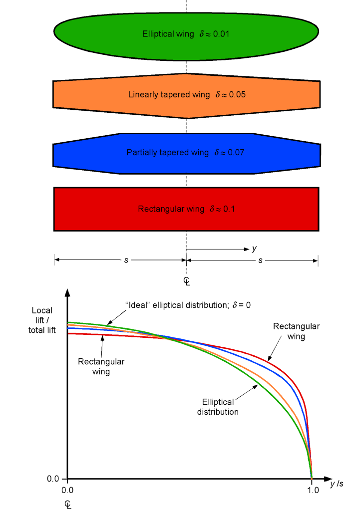
The shape of the wing (i.e., its planform) will affect the distribution of lift and the formation of the trailing vortex system, hence the magnitude of the induced drag on the wing. The idea is to use variations in wing chord along the span and perhaps wing twist and airfoil sections to approximate the ideal elliptical spanwise loading closely and minimize the value of . The actual effective aspect ratio of the wing can also be improved somewhat by paying attention to the shape of the wing tips, which can lower the values of if they are suitably shaped, e.g., with more rounded contours or perhaps with the addition of a winglet.
Incorporating Wing Twist
In the lifting line theory, wing twist affects the circulation distribution by altering the local geometric angle of attack along the span, which modifies the local lift coefficient. The effective angle of attack at any spanwise location is now given by
(85) 
where  is the local geometric angle of attack, including the effect of twist, and the induced angle of attack
  is
is
(86) 
Wing twist, denoted as  , modifies the geometric angle of attack by
(87) 
where  is the root angle of attack. Substituting this, the effective angle of attack becomes
(88) 
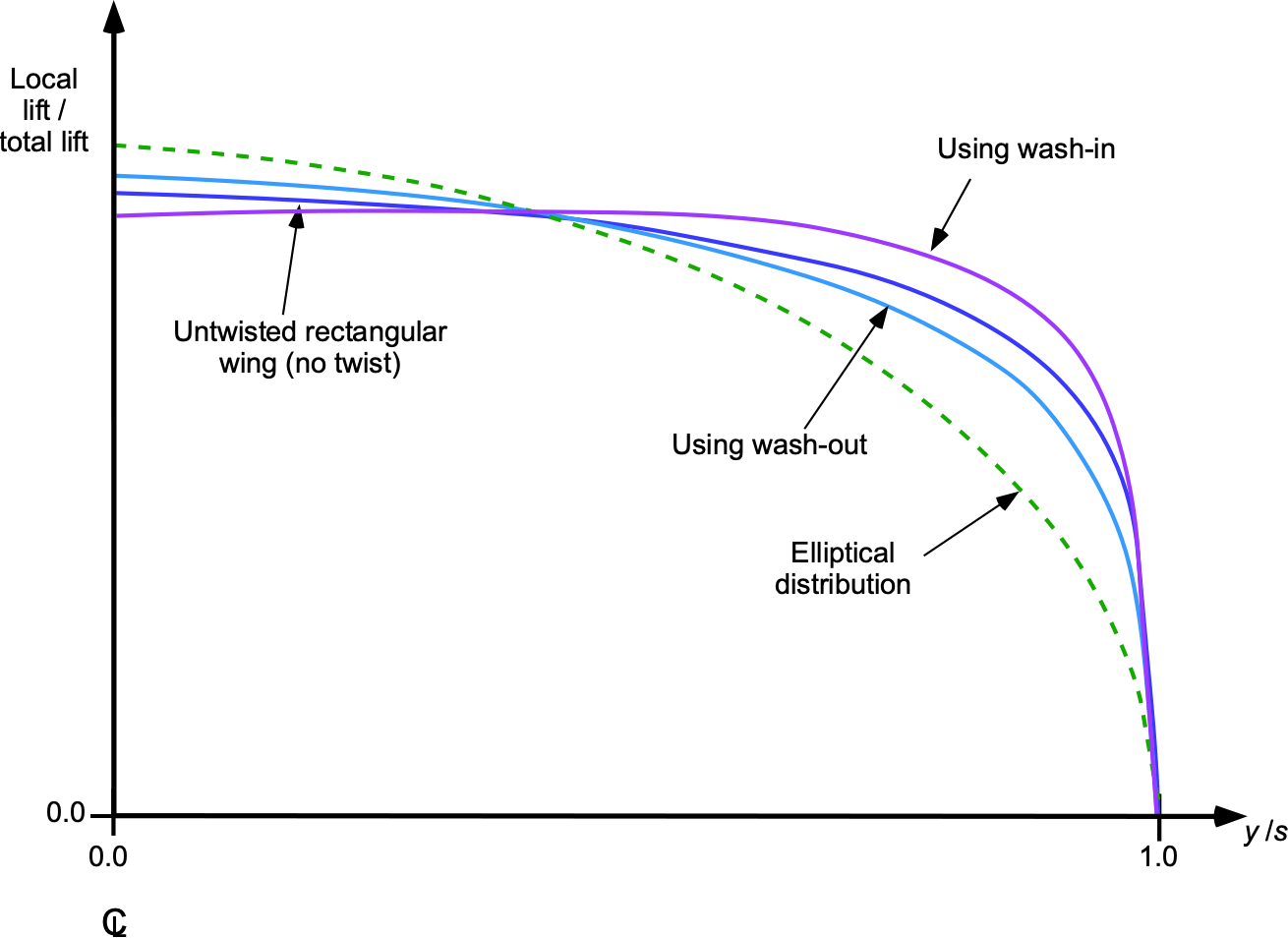
Notice that in the case of no twist, i.e., ( ), the geometric angle of attack is constant, and the circulation distribution depends only on the wing shape and induced effects. In the case of wash-out, i.e., decreases toward the tip, this reduces lift at the wingtips, redistributes lift inboard, as shown in the figure below, and also decreases induced drag. If the wing has wash-in, i.e., increases toward the tip (which is unusual), it increases lift at the wingtips, leading to higher induced drag. Twist allows designers to optimize the lift distribution and induced drag for specific flight conditions.
Interference Effects
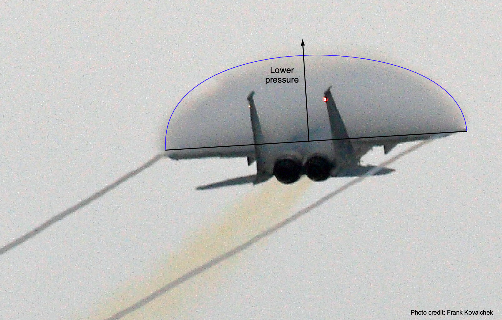
The photograph below illustrates the nature of the spanwise loading over a wing from the process of natural condensation in the low-pressure zones, which is nominally elliptically distributed, even on this relatively low aspect ratio wing. The highest lift (highest pressure difference) is at midspan, and the lowest lift (lowest pressure difference) is at the wing tips. The problem is, however, that even minor deviations from the ideal elliptical form can result in higher induced drag from the wing. Such variations can occur because of interference effects on the wing from the fuselage, engines, undercarriage, external stores, and other components.
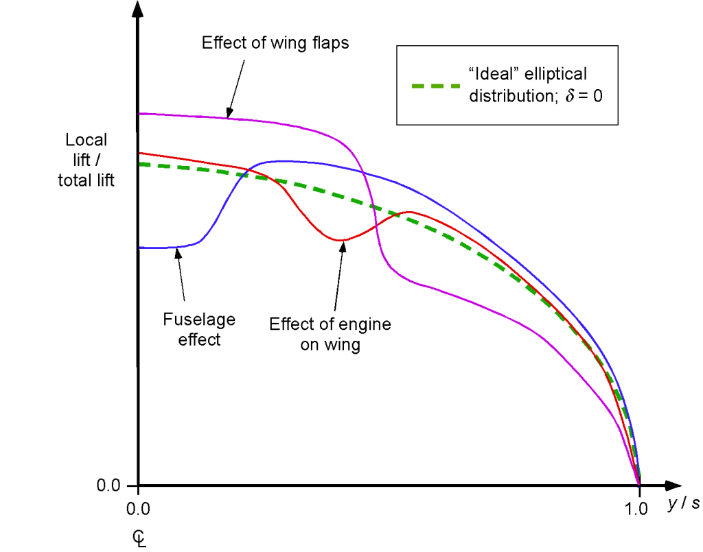
Examples of the effects of spanwise interference are shown in the figure below, which are for the same approximate value of total wing lift. Notice that the fuselage can produce significant deviations from the ideal elliptical form, perhaps increasing the value of to over 1.15. However, local effects along the wing, such as those caused by the aerodynamic interference effects produced by an engine, tend to have a minor impact on the value of .
 .
.What is aerodynamic twist?
Aerodynamic twist refers to the variation in the airfoil’s camber or thickness distribution along the wing span, which alters the local zero-lift angle of attack, , such as using a different airfoil section. Unlike geometric twist, which physically pitches the wing sections, aerodynamic twist modifies the airfoil shape to tailor the lift characteristics. By modifying , the effective angle of attack and, consequently, the spanwise lift distribution can be modified. In the context of lifting line theory, aerodynamic twist directly impacts the governing equation by introducing a spanwise variation in . This changes the effective angle of attack, which determines the local lift coefficient and the distribution of circulation. The primary advantage of aerodynamic twist is its ability to achieve specific spanwise loading patterns, such as near-elliptic lift distributions, without changing the wing’s physical orientation. This minimizes induced drag, optimizes load redistribution, and enhances performance for non-elliptic planforms.
Additionally, aerodynamic twist improves stall behavior by reducing lift near the tips, ensuring the wing root stalls first. It also provides flexibility in wing design, as it does not require a physical twist of the wing sections like a geometric twist. By incorporating aerodynamic twist into lifting line theory, designers can achieve a better balance between aerodynamic efficiency, structural feasibility, and flight performance.
Induced Drag Reduction Using Winglets
Winglets reduce the induced drag of finite wings by modifying the location and structure of the trailed vortex system generated as a consequence of lift generation. Although winglets increase the wing’s wetted surface area and give a small increment to overall skin friction and profile drag, they typically produce a net reduction in total airplane drag for no increase in wingspan. This tradeoff explains the widespread adoption of winglets on modern commercial airliners as an effective strategy for reducing drag and saving fuel.
In the following analysis, the wing and its wake are modeled using a classical lifting-line horseshoe vortex system, modified to include winglets by geometrically displacing the trailing vortex legs, as illustrated in the figure below. The induced velocity is evaluated at the mid-span of the wing. While this effective span winglet theory does not represent the spanwise variation in downwash, it provides a useful approximation of the total induced drag using the principles of the Biot-Savart law. It highlights the aerodynamic benefit of winglets through their influence on the geometry of the trailing vortex system.
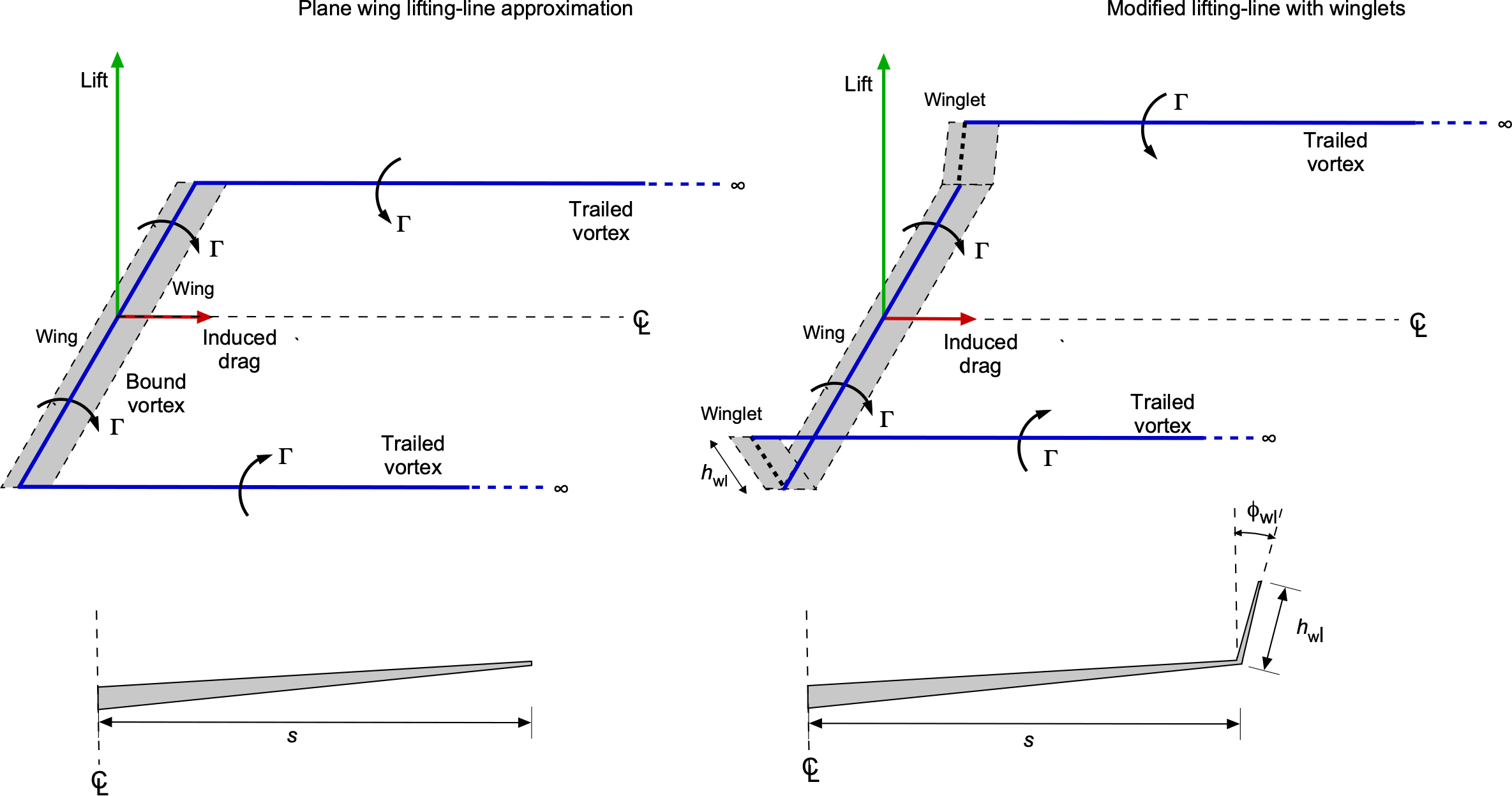
The winglet itself is assumed to generate no lift or drag; its effect is modeled purely as a geometric shift in the starting position of the tip vortex, effectively moving it farther from the lifting wing. As such, this model isolates the influence of vortex positioning on the downwash field (albeit a mild violation of Helmholtz’s laws) without accounting for the winglet’s detailed aerodynamic behavior or the tip vortex’s roll-up. The wing tip vortices are still modeled as semi-infinite straight filaments extending downstream, so the induced vertical velocity field can be calculated using the Biot-Savart law.
When the wing has regular tips (no winglets), the trailing vortices originate in the plane of the wing at  , the effects of any dihedral angle being neglected. The induced vertical velocity at mid-span is
(89) 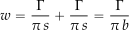
where is the semi-span, representing the lateral displacement from the mid-span at  to the origin of the tip vortices. Now, consider the case when the winglets relocate the vortex tips along a length
  at a cant angle
  from the vertical. The trailed vortex filaments, i.e., the wing tip vortices, now start from
  . Notice that this approach assumes that the spatial separation of the trailing vortex system governs induced drag. This formulation is consistent with Prandtl-Jones minimum induced drag theory,[7] in which the induced drag is inversely proportional to the distance between the trailing vortices.
Using the Biot-Savart law, the vertical velocity induced at mid-span by one vortex leg is
(90) 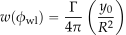
where
(91) 
Including both tip vortices, the induced velocity becomes
(92) 
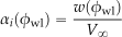
which gives the induced angle of attack as
(93) 
The lift generated by the wing is
(94) 
As a consequence, the induced drag is
(95) 
and so compared to the baseline wing without the winglet, then
(96) 
where  .
.
In coefficient form, an effective aspect ratio can also be defined based on the inverse of the downwash ratio (to reflect a correct reduction of induced drag), i.e.,
(97) 
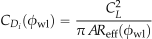
where is the baseline aspect ratio of the wing without the winglet. Therefore, the induced drag coefficient becomes
(98) 
Special cases include:
- No winglet:
(99)

- Vertical winglet:
(100)

- Flat winglet (full span extension):
(101)

Minimizing induced drag from the use of a winglet corresponds to maximizing  , which depends on the effective location of the trailed vortex system. Define the geometric function
(102) 
Expanding and simplifying this gives
(103) 
This function is minimized for a given winglet length when  is minimized, i.e., at
(104) 
which corresponds to a downward-pointing winglet. However, such a configuration is impractical because of ground clearance, among other limitations. Therefore, to determine the optimum cant angle under the current assumptions, define the performance metric
(105) 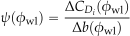
which measures induced drag reduction per unit increase in span. The induced drag reduction is
(106) 
and the effective span added by the winglet is
(107) 
Substituting yields  in ratio form, i.e.,
(108) 
Maximizing corresponds to solving
(109) 
which leads to a transcendental equation in that must be solved numerically. The results summarized in the figure below indicate that the reduction in induced drag increases with the cant angle and winglet length but diminishes beyond a cant angle of approximately  .
.
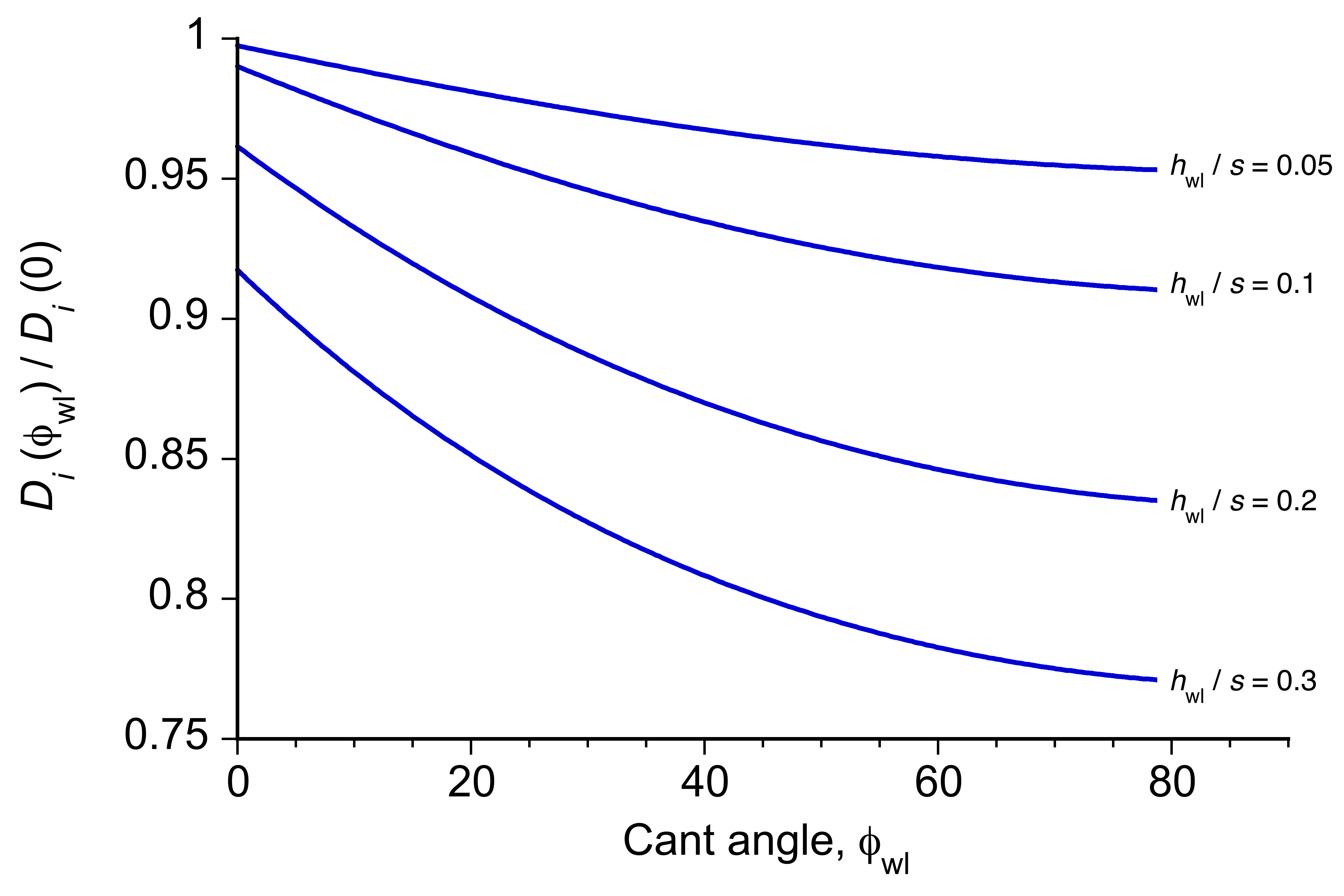
 and cant angle .
A commonly used approach in airplane performance analysis to estimate the effect of a winglet is to use a linear correction to the aspect ratio of the form
(110) 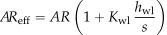
where  is the corrected or “effective” aspect ratio, is the height of the winglet, and
  is a coefficient that depends on the winglet geometry. This expression is widely used in preliminary design because of its simplicity.
This model, given by Eq. 110, can be reconciled with the theoretical effective span winglet theory by performing a Taylor expansion of the more general result. Recall that the effective aspect ratio based on the trailed wingtip vortex geometry is
(111) 
where  . Expanding this expression for small
  gives
gives
(112) 
Comparing this expansion with Eq. 110, the linear winglet correction coefficient is identified as
(113) 
This result shows that the linear model is simply a first-order approximation to the vortex-induced effective span theory. For a typical cant angle of  , this yields
  , which aligns with values often cited in the literature for a classic winglet. Therefore, while Eq. 110 provides a convenient approximation; the full geometric expression is more accurate, especially for larger winglet lengths or varying cant angles. In both cases, however, increasing the spatial separation of the trailed vortices, whether through increased span and/or vertical offset, results in reduced induced drag on the wing, which is consistent with the proven aerodynamic effects of winglets.
Worked Example #4 – Aerodynamic benefit of a typical winglet
Consider a wing with semi-span = 30 ft and a winglet of height = 2 ft, giving  . If the winglet has a cant angle of
  , estimate the improvement in effective aspect ratio using both the vortex-induced effective span theory and its linear approximation. Then, assuming the wing has a baseline aspect ratio of
  , a wing reference area = 124 m, cruise lift coefficient = 0.5, and fuel flow rate of 2.6 kg/s at cruise, determine the reduction in induced drag using the winglet and the corresponding fuel savings over a 3-hour flight. Assume the induced drag accounts for 40% of the total drag.
Show solution/hide solution.
Using the vortex-induced effective span model, then
(114) 
Putting in the values gives
(115) 
For comparison, using the linear approximation gives
(116) 
The vortex-induced effective span model predicts an effective aspect ratio of  . The ratio of induced drag coefficients is
(117) 
This corresponds to an 8.6% reduction in induced drag. If the induced drag is 40% of the total drag, then the total drag reduction is
(118) 
The corresponding reduction in fuel flow rate is
(119) 
Therefore, over a 3-hour flight (10,800 s), the total fuel saved is
(120) 
Notice that a modest 2-foot winglet at a 25 cant angle yields a 9.4% increase in effective aspect ratio (vortex-induced effective span mode), leading to an 8.6% reduction in induced drag and a 3.4% reduction in total drag. Over a typical 3-hour flight, this translates to nearly one metric ton of fuel saved, highlighting the aerodynamic and operational value of even modest winglet designs.
Biplane Wing Theory
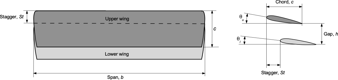
While there are few biplane types of airplanes flying today, other than in general aviation, their aerodynamics are interesting and instructive because of the dual-lift system and mutual aerodynamic interference between the two wings. A simple biplane consists of two wings, typically aligned almost vertically one above the other, and spaced apart by a vertical distance called the gap, , as shown in the figure below. Each wing can be assumed to have a span and a chord , although the wings may have different spans and chords. The wings may be offset horizontally by a geometric parameter called stagger,  . Another geometric parameter, the decalage angle, refers to the angular offset between the incidences, or pitch angles, of a biplane’s upper and lower wings. If the upper wing has an incidence angle
  and the lower wing
  , then the decalage angle,
  , is defined as the difference
(121) 
History
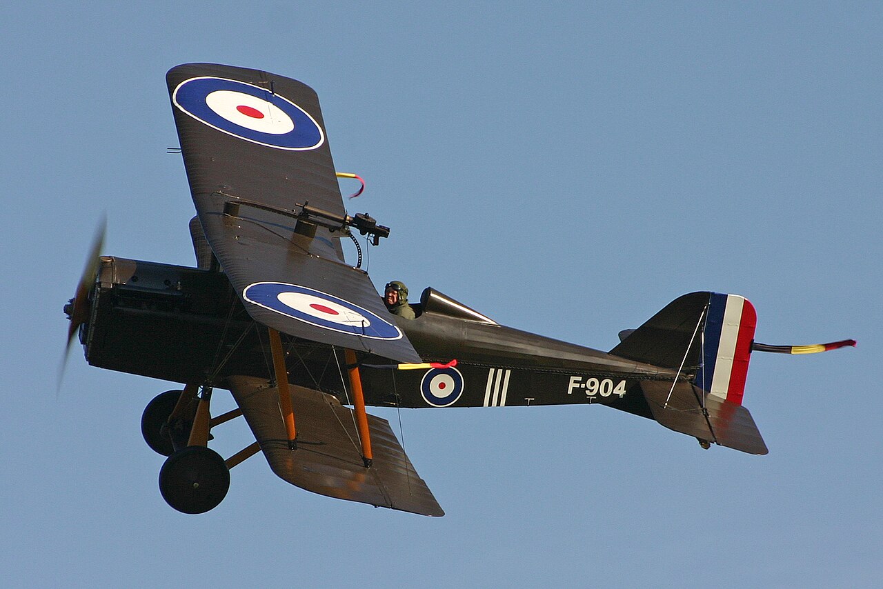
There are subtle differences between biplanes that have been built over time. One of the most iconic biplanes of WWI, the Sopwith Camel, employed moderate positive stagger and slight positive decalage, improving forward visibility and enhancing longitudinal trim. Thanks to its relatively short wingspan, the Camel was known for its agility and tight turning radius. The Royal Aircraft Factory SE5a, as shown in the photograph below, featured a more pronounced stagger and relatively large gap. This configuration reduced interference drag and gave it more airspeed in level flight.
The Curtiss JN-4 “Jenny” was used primarily as a trainer during WWI. Its small wing gap and relatively low stagger led to greater aerodynamic interference. However, its docile handling characteristics were ideal for training, though its low performance reflected the compromise made in aerodynamic efficiency. The Fokker D.VII was more unusual because it used minimal stagger but a large gap. This design significantly reduced the interference drag, and it was one of the few biplanes that was nearly as efficient as a monoplane.
A modern example of a biplane is the Pitts Special, a compact, high-performance aerobatic aircraft. Unlike early biplanes, the Pitts Special prioritizes extreme maneuverability and high agility. It features positive wing stagger and decalage, improving pilot visibility and trim stability during upright flight. The aircraft features low-aspect-ratio wings and symmetric airfoils, which facilitate rapid roll rates in both upright and inverted attitudes. In such designs, the induced drag is not minimized; instead, the aerodynamic layout is optimized for maneuverability, agility, and light control response under high-loading maneuvers. The Pitts Special exemplifies how biplane configurations persist in niche roles where their unique design features offer specific performance advantages.

Other biplanes, such as the Christen (Aviat) Eagle and the Waco YMF-5, further demonstrate the continued relevance of the biplane layout in specialized applications. The Christen Eagle, also designed for aerobatics, features similar structural compactness and maneuvering performance as the Pitts. The Waco YMF-5, in contrast, is a modern reproduction of a 1930s-era luxury sport biplane, emphasizing nostalgic appeal and stable touring characteristics rather than aerobatic performance. These examples highlight the biplane configuration’s versatility in recreational and competitive aviation, despite the overwhelming dominance of monoplanes in mainstream civil and military aviation.
Aerodynamics of Biplanes
In a biplane configuration, each wing generates a trailing vortex system, producing a downwash field in the wake. This downwash alters the local flow field encountered by the other wing, effectively reducing its angle of attack. Consequently, the lift produced by each wing is lower than it would be if the wings operated independently in isolation. This mutual aerodynamic interference is a defining feature of biplane aerodynamics; it becomes more pronounced as the vertical gap between the wings decreases or as their stagger and decalage angles are reduced.
The interference reduces the total lift for a given geometric angle of attack. It increases the induced drag because the downwash fields reinforce each other, contributing to a greater wake deflection. Consequently, the aerodynamic efficiency of the biplane is significantly lower than that of an equivalent monoplane with the same total area and span. The extent of this degradation can be quantified through theoretical models, such as Prandtl’s biplane interference formula or Glauert’s extensions of lifting-line theory, which incorporate correction factors for gap, stagger, and wing loading distribution. Understanding these interference effects is crucial for evaluating the performance of historical biplane designs and assessing the trade-offs between structural compactness and aerodynamic efficiency.
Classic Theory
Ludwig Prandtl was the first to address the aerodynamics of biplanes, deriving a formula for the induced drag, i.e.,
(122) 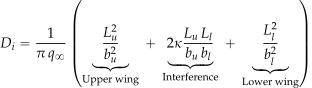
where  and
and  refer to the lift and span of the upper wing, and
  and
and  refer to the lift and span of the lower wing, respectively. The term
  is a biplane interference factor. While not all biplanes have the same wingspan, if
  and
and  , then
(123) 
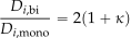
The ratio of biplane to monoplane induced drag is then
(124) 
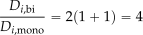
In the worst case, where  , the biplane has four times the induced drag of an equivalent monoplane, i.e.,
(125) 
More typically, if  to
to  , then
(126) 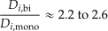
This latter result highlights why biplanes, while structurally efficient and compact, suffer aerodynamically from mutual interference between the two wings. The theory shows that they have a lift-to-drag ratio less than half that of a monoplane.
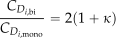
The same result can be determined in terms of aerodynamic coefficients, perhaps a more general and familiar approach, i.e.,
(127) 
where  and
and  are the lift coefficients of the upper and lower wings, respectively, and is the aspect ratio of each wing (assumed equal). If the wings are identical and equally loaded, so that
  , then
(128) 
The induced drag coefficient of a monoplane with the same lift coefficient and aspect ratio is
(129) 
Therefore, the ratio of induced drag for the biplane to the monoplane becomes
(130) 
General Theory
Other early aerodynamicists, such as Hermann Glauert and Max Munk, developed models to quantify further the biplane interference effect using extensions of lifting-line theory. For a monoplane wing, the three-dimensional lift-curve slope can be shown to be
(131) 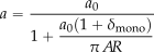
where  is the two-dimensional value (often referred to as , and
  accounts for the deviation of the spanwise loading from the elliptical. For a biplane with no stagger or decalage, an additional interference term appears as
(132) 
The value of is referred to as an aerodynamic interference factor, so a penalty that increases as the gap, , decreases.
For the monoplane, the induced drag coefficient is
(133) 
The lift coefficient is
(134) 
and so substituting gives
(135) 
where the aspect ratio is  .
.
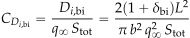
For the biplane, with symmetric lift sharing and span for each wing and total lift  , the induced drag is
(136) 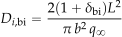
and the corresponding drag coefficient is
(137) 
Using  , then
(138) 
Assuming  , then
(139) 
This latter result shows that the induced drag coefficient for a biplane is increased by a factor of four relative to a monoplane with the same aspect ratio, assuming symmetric lift sharing, equal lift coefficient, and  .
.
Munk’s Stagger Theorem
Munk’s Stagger Theorem is a classical result from early biplane theory, addressing the induced drag characteristics of multiple lifting surfaces arranged with longitudinal stagger. The theorem was formulated by Max Munk in the 1920s and remains a foundational concept in theoretical aerodynamics for multi-wing configurations. It states: “For two or more coplanar lifting surfaces with the same total span and the same total circulation, the induced drag of the system is independent of the stagger between the wings, provided that the wake remains planar and aligned with the freestream.”
As Munk states, this result holds under several, perhaps idealized, assumptions. The flow must be steady, incompressible, inviscid, and irrotational. All lifting surfaces are assumed to lie in the same horizontal plane, with no vertical separation between them. The total span and total bound circulation of the system are held constant. The wake shed by the lifting surfaces is assumed to remain flat and aligned with the freestream direction, and the flow is modeled using classical lifting-line theory.
In lifting-line theory, the induced drag is expressed as
(140) 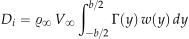
where is the bound circulation at the spanwise location , and is the downwash induced by the trailing vortex system. When the total span and circulation are held fixed, introducing a fore-aft offset between the wings, known as stagger, modifies the local circulation distribution and downwash but leaves the total integral unchanged. Because induced drag depends only on this integral, it remains invariant under idealized changes in stagger.
The local induced angle of attack on each wing is affected by both its own trailing vortices and those of the other wing. The net induced angle of attack at spanwise location is
(141) 
where  arises from the downwash induced by the other wing. For a vortex filament at vertical gap and horizontal stagger
  , the mutual downwash is approximated by
(142) 
As stagger increases, this induced velocity becomes more asymmetric between the wings, enhancing the induced angle of attack and, therefore, increasing induced drag.
In terms of a Fourier-mode representation of the spanwise circulation, the induced drag is given by
(143) 
where are the coefficients of the loading modes, and  is a stagger-dependent interference term. Because increases with stagger, it follows that
  . In the non-staggered case (
 ), the trailing vortices from the upper and lower wings are vertically aligned, and their downwash fields partially cancel each other. In contrast, stagger skews the wake and increases mutual interference, thereby enhancing the overall downwash and, consequently, the induced drag.
Munk’s theorem implies that one cannot simply reduce induced drag on a biplane by staggering its wings. Although stagger changes local aerodynamic interference, the total induced drag remains the same if the total circulation and span remain the same. Consequently, modifications such as introducing vertical separation (gap), adjusting twist, or redistributing circulation spanwise are required to reduce induced drag in multi-wing configurations in a meaningful manner.
It is essential to recognize the limitations of the theorem, as it applies only within the framework of lifting-line theory. In real flows, effects such as mutual wake distortion introduce deviations from the idealized assumptions. Three-dimensional wake behavior at high angles of attack can also invalidate the assumption of a flat, undisturbed wake. Nonetheless, Munk’s Stagger Theorem offers a valuable theoretical insight into the behavior of coplanar lifting surfaces and remains a benchmark in the aerodynamic analysis of biplanes and multiplanes.
Decalage
Decalage refers to the angular difference in incidence or geometric pitch between the upper and lower wings of a biplane. This geometric offset directly affects the lift distribution, typically increasing the lift on the wing with greater incidence. However, decalage also introduces asymmetric aerodynamic interference. The downwash produced by one wing modifies the effective angle of attack on the other in a non-uniform manner, depending on the gap, stagger, and relative circulation strengths. Consequently, the mutual influence between the wings becomes more complex, and the induced drag may increase.
The interference factor , which accounts for the degradation in aerodynamic efficiency because of wing–wing interaction, must be carefully re-evaluated when decalage is present. In addition to altering lift sharing, decalage significantly impacts the pitching moment and longitudinal trim, and must be chosen with consideration of both aerodynamic performance and stability requirements.
Design Trades with Biplanes
Despite Munk’s theorem, actual biplane configurations often incorporate stagger and decalage for practical reasons that extend beyond minimizing induced drag. Stagger can improve the pilot’s overall visibility by moving the upper wing forward. It also allows for shorter and lighter interplane struts, which reduce structural weight and drag. Adjustments in stagger and decalage can also help shift the center of pressure to achieve desirable trim and stability characteristics. In addition, physical constraints can influence the choice of wing placement.
Positive decalage, in which the upper wing is set at a higher geometric angle of incidence than the lower wing, is commonly used to achieve longitudinal trim or pitch stability. This configuration generates more lift from the upper wing than from the lower wing. As a result, the aerodynamic center shifts, and the aircraft gains more favorable moment characteristics for trimmed, stable flight.
Aircraft with short wings and low aspect ratio experience reduced roll damping compared to longer-span designs. Roll damping arises from the differential lift generated across the wing span during a rolling rate motion, with one wing experiencing an increased angle of attack and the other a decreased one. This effect is pronounced on high-aspect-ratio wings, which generate significant aerodynamic damping in roll, e.g., a sailplane. However, the roll damping is much smaller with two short wings rather than one longer and higher aspect ratio wing of the same wing area. This characteristic is advantageous in aerobatic aircraft, such as the Pitts Special, where rapid roll response and minimal resistance to roll acceleration are essential for precise maneuvering. The two wings give the needed lift, and the low roll damping contributes directly to the aircraft’s high agility.
Worked Example #5 – Biplane aerodynamic performance
A biplane has two identical wings, each with span = 6 m and chord = 1.2 m. The total mass of the airplane is  = 1,000 kg. The aircraft flies at MSL ISA conditions at an airspeed of = 80 mph. Assume: 1. Two-dimensional lift curve slope: = 2. 2. Span efficiency factor for monoplane:
  = 0.05. 3. Interference correction factor for biplane: = 0.30. 4. Effective span efficiency factor for the biplane:
  = 0.2.
- Determine the lift coefficient based on the total reference area
 .
. - Compute the lift curve slope of separate monoplane wings,
 , and for the biplane,
  .
. - Determine the induced drag coefficient for the separate monoplanes,
 , and for the biplane
  .
. - Comment on the aerodynamic efficiency of this biplane compared to a monoplane of the same span and total area.
Show solution/hide solution.
- The area of one wing is
(144)

so the aspect ratio is
(145)
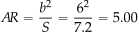
The total reference area for the biplane is
(146)

The total lift required equals the airplane’s weight, i.e.,
(147)

The airspeed is
 , so the dynamic pressure is
(148)

The lift coefficient is then
(149)

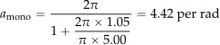
- The lift curve slope for a monoplane wing with span efficiency
 is
is
(150)
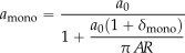
Substituting the values gives
(151)
The biplane’s lift curve slope, accounting for interference, is
(152)
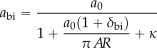
Substituting the values gives
(153)

- The induced drag coefficient for the monoplane is
(154)

The induced drag coefficient for the biplane is
(155)

- Compared to two separate monoplane wings, the biplane has a lower lift curve slope (
 vs.
vs.  ) and a significantly higher induced drag coefficient (
 vs.
vs.  ). The aerodynamic penalty comes from mutual downwash interference between the wings, quantified by and . Although compact, the biplane is substantially less efficient in cruise than an equivalent monoplane.
Note on Triplane Configurations
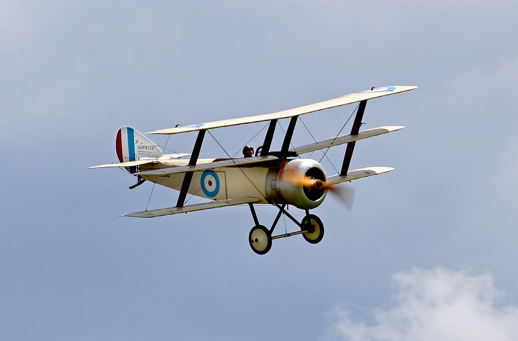
A triplane, a relatively rare type of airplane, features an additional lifting surface positioned above or below the existing biplane configuration. As shown in the photograph below, the Sopwith Triplane was a British single-seat fighter aircraft designed and manufactured by the Sopwith Aviation Company during WW1. It has the distinction of being the first military triplane to see operational service. The motivation for a triplane is to increase the total wing area without increasing the span, which benefits both structural stiffness and maneuverability. However, interference effects become more severe with the third wing. In this case, each wing contributes to the downwash seen by the others, and the mutual interference becomes more complex. Theoretical treatments typically model the triplane as three lifting lines, where each line experiences downwash induced by the other two.
The induced drag of a triplane can be estimated by extending lifting line theory to three wings. If each of the three wings carries an equal share of the aircraft’s weight, i.e.,  =
=  and the span is , then the induced drag is approximated as
(156) 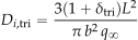
where  is an effective span efficiency factor for the triplane configuration. The factor of 3 arises because the three lifting surfaces contribute cumulatively to the total induced drag and experience mutual aerodynamic interference. In general,
(157) 
indicating a progressive loss in aerodynamic efficiency compared to a biplane and monoplane. In coefficient form, using a total reference area  , the induced drag coefficient becomes
(158) 
This latter result shows that while the triplane has the same functional form for  as a monoplane, the span efficiency factor is significantly higher because of the added interference and downwash effects from the multiple wings. The net result is a higher induced drag penalty for the same lift coefficient and aspect ratio.
The Fokker “Dr.I” Triplane, the most famous triplane, used short spans and closely spaced wings. It had an impressive roll rate and climb capability, but suffered from high drag, which limited its speed and maneuverability. Its triplane configuration reflected a specific design solution focused on turning agility in dogfights. Triplanes had a brief period of popularity during WWI but were quickly abandoned thereafter as monoplane structures improved and interference drag became better understood.
Flying Wings
Flying wings, also known as tailless aircraft, are a distinctive and relatively unusual class of aircraft in which the fuselage and empennage, as well as all the flight control surfaces, are fully integrated into the wing structure, thereby eliminating the need for a traditional tail. This design offers several advantages, including reduced drag, a lower structural empty weight fraction, and an increased payload fraction. The Northrop Grumman B-2 Spirit stealth bomber is a prime example of a modern flying wing design, which cruises just below the speed of sound. Its smooth, blended aerodynamic surfaces minimize drag and also reduce its radar cross-section, making it highly effective in evading enemy radar. However, the tailless flying wing configuration also introduces unique technical challenges that must be addressed to ensure acceptable flight performance, particularly in terms of its directional stability and control.
Aerodynamics of Flying Wings
Flying wing designs benefit from reduced parasitic drag compared to conventional airplanes of similar size and weight. Their continuous wing surfaces and carefully shaped aerodynamic profiles eliminate many of the typical sources of drag and flow interference found on traditional configurations. However, while conventional wing design has long aimed for an elliptical spanwise lift distribution to minimize induced drag, flying wings require a slightly different approach. The absence of a fuselage and tail surfaces means that the spanwise lift distribution must be tailored not only for good aerodynamic efficiency but to ensure adequate stability and control.
In contrast to the elliptical spanwise lift distribution, which is ideal for minimizing induced drag on conventional wings, flying wings typically employ a bell-shaped spanwise loading, as illustrated in the schematic below. This distribution concentrates more lift toward the inboard sections of the wing, reducing structural bending moments and enabling a lighter wing design. However, this comes at the cost of increased induced drag. One way to offset this penalty is to use a slightly longer wing with a higher aspect ratio, within the constraints of an allowable bending moment and wing weight, thereby regaining aerodynamic efficiency while maintaining overall structural efficiency.
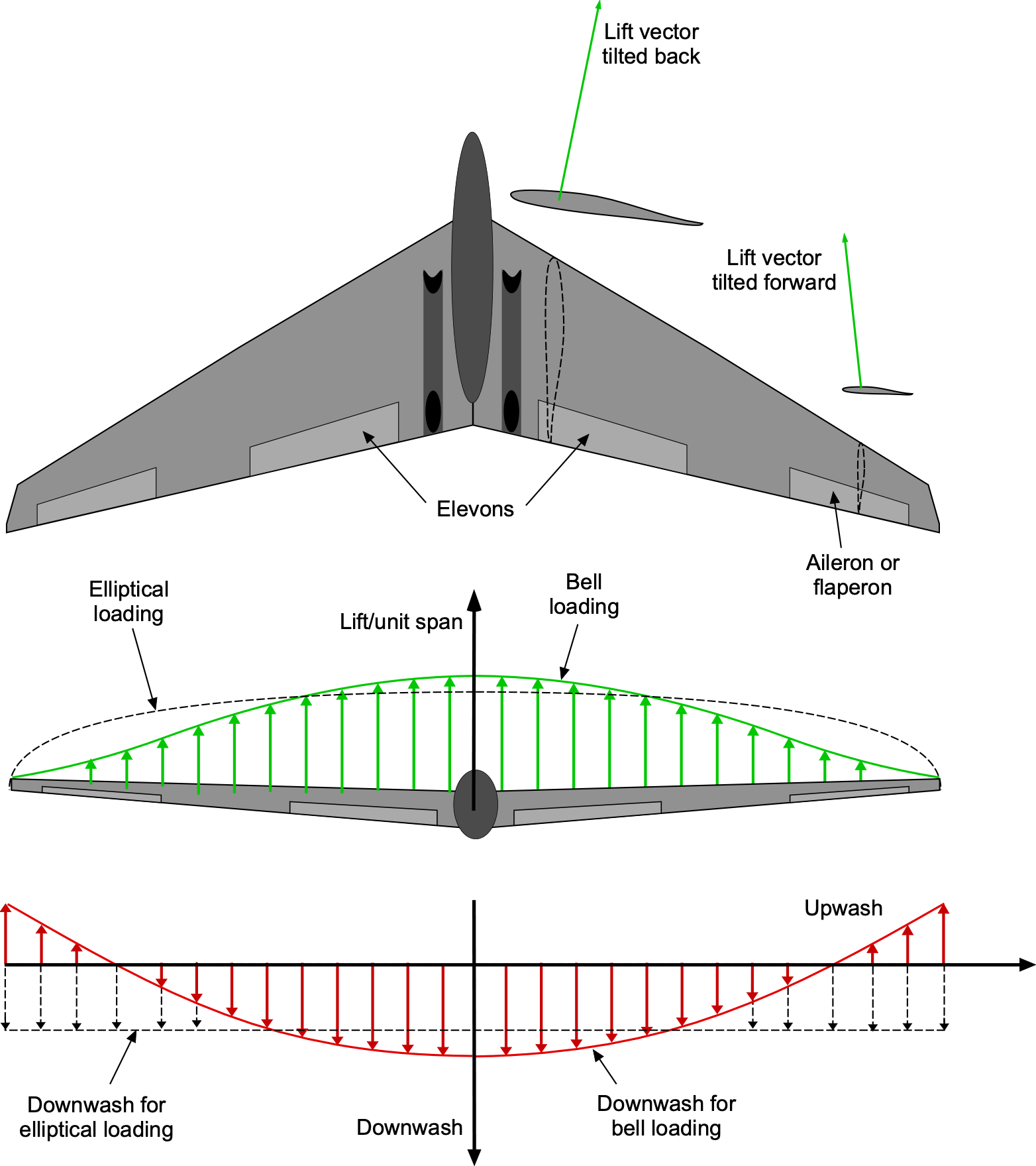
But creating such a bell-shaped spanwise loading, which is achieved through suitable variations in wing chord and twist, serves another important purpose in that it establishes upwash regions over the outer wing panels. This upwash generates forward-acting lift vectors in those regions, effectively producing negative induced drag. It is this forward-acting lift force at the wingtips that provides the flying wing with essential directional (yaw) stability and control. In addition, it leads to proverse yaw in response to aileron or flaperon inputs,[8] a feature critical for flying wings, which lack a vertical tail and rudder.
Bell-Shaped Loading
The aerodynamic consequences of the bell-shaped spanwise loading require further exposition. A starting point is the extended spanwise loading solutions discussed by Prandtl in 1933, which stemmed from Munk’s original formulation of the lifting-line theory,[9] who concluded that if the wing span or aspect ratio is not a design constraint, other forms of the spanwise lift distribution may help optimize the aerodynamic and structural efficiency of a wing. However, he makes no mention of any application to tailless flying wings.
Prandtl introduced a more general spanwise circulation loading function given by
(159) 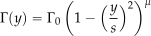
where = 1/2 gives the classic elliptical loading and = 3/2 gives a “bell-shaped” loading. The bell-shaped loading distribution has a higher peak  near the wing root compared to the elliptical loading. It then quickly decreases towards the wingtip, where the lift over the outer part of the wing is much lower, thereby giving it the characteristic “bell shape,” as shown in the figure below.
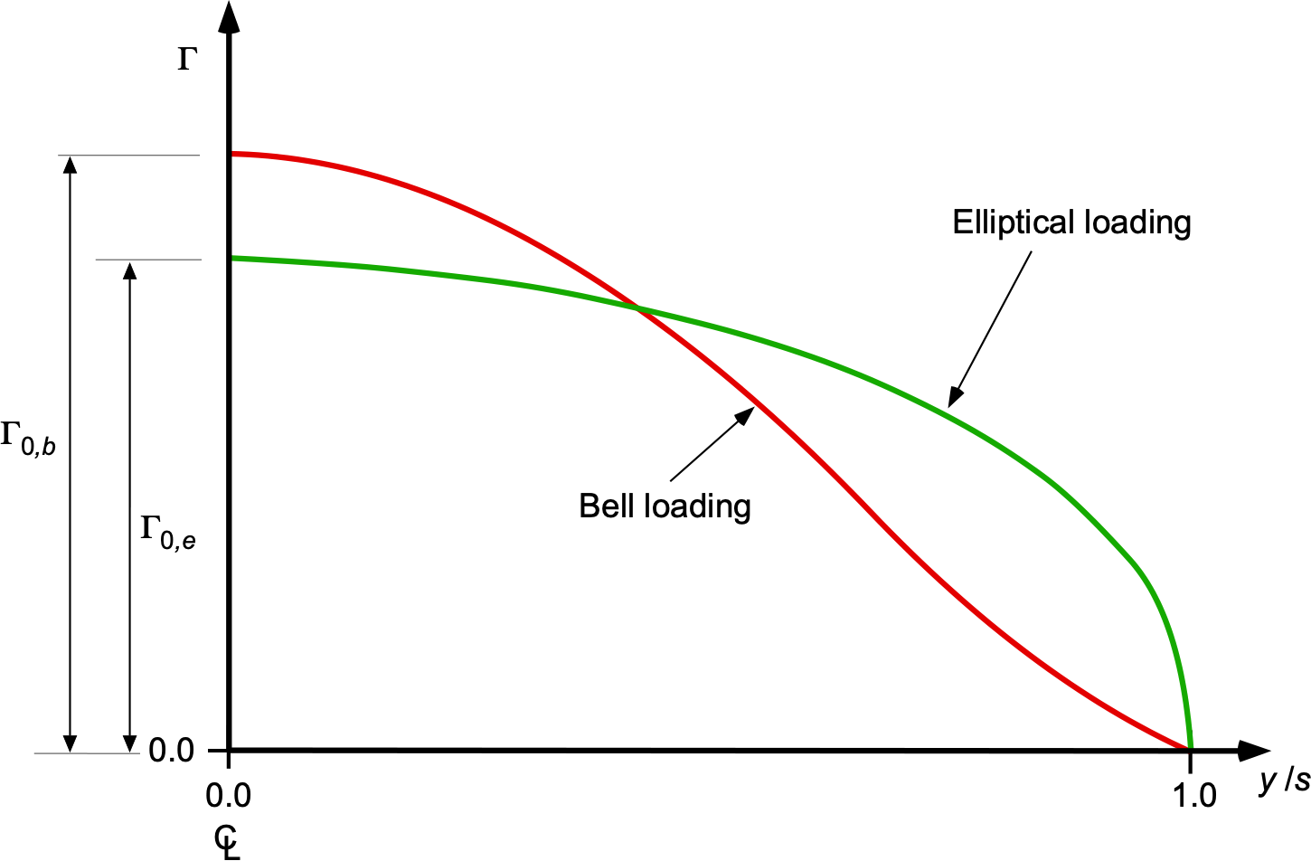
Therefore, the two idealised spanwise circulation loadings of interest for further comparative analysis are the classical elliptical form (as a reference) with = 1/2, i.e.,
(160) 
and the bell-shaped form with = 3/2, i.e.,
(161) 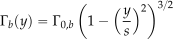
where  and
and  are the respective loadings (circulation values) at mid-span. A standard symmetric wing of semi-span
  is assumed.
Downwash
There is a non-uniform downwash over the wing with the bell-shaped spanwise loading (compared to the uniform downwash obtained with the elliptical loading), with an upwash being produced over the outer part of the wing. For the well-known elliptical span loading, the downwash, , is constant across the span, i.e.,
(162) 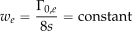
For an untwisted elliptical planform with uniform downwash, it also results in a constant induced angle of attack and a constant local lift coefficient across the span, representing the minimum induced drag configuration for the wing.
The downwash corresponding to the bell-shaped loading can be obtained from the lifting-line method discussed previously, which expresses the circulation as
(163) 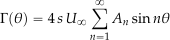
where the coefficients can be determined from the prescribed loading. The bell spanwise loading distribution is
(164)
Using the standard transformation with the lifting line theory that  where
where  , then
  . Furthermore, using the trigonometric identity that
  , then only the first and third harmonics appear in the loading distribution, i.e.,
(165) 
Matching coefficients gives
(166) 
For any general circulation distribution, then the downwash is
(167) 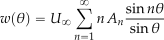
and substituting for the bell-shaped loading gives
(168) 
Using the trigonometric identity that  , then
 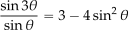 , and so
(169) 
 , then
 (170) 
This result means that the downwash with the bell-shaped spanwise loading is a maximum at the wing root and becomes an upwash at the tip outboard of =  = 0.707, as shown in the figure below.
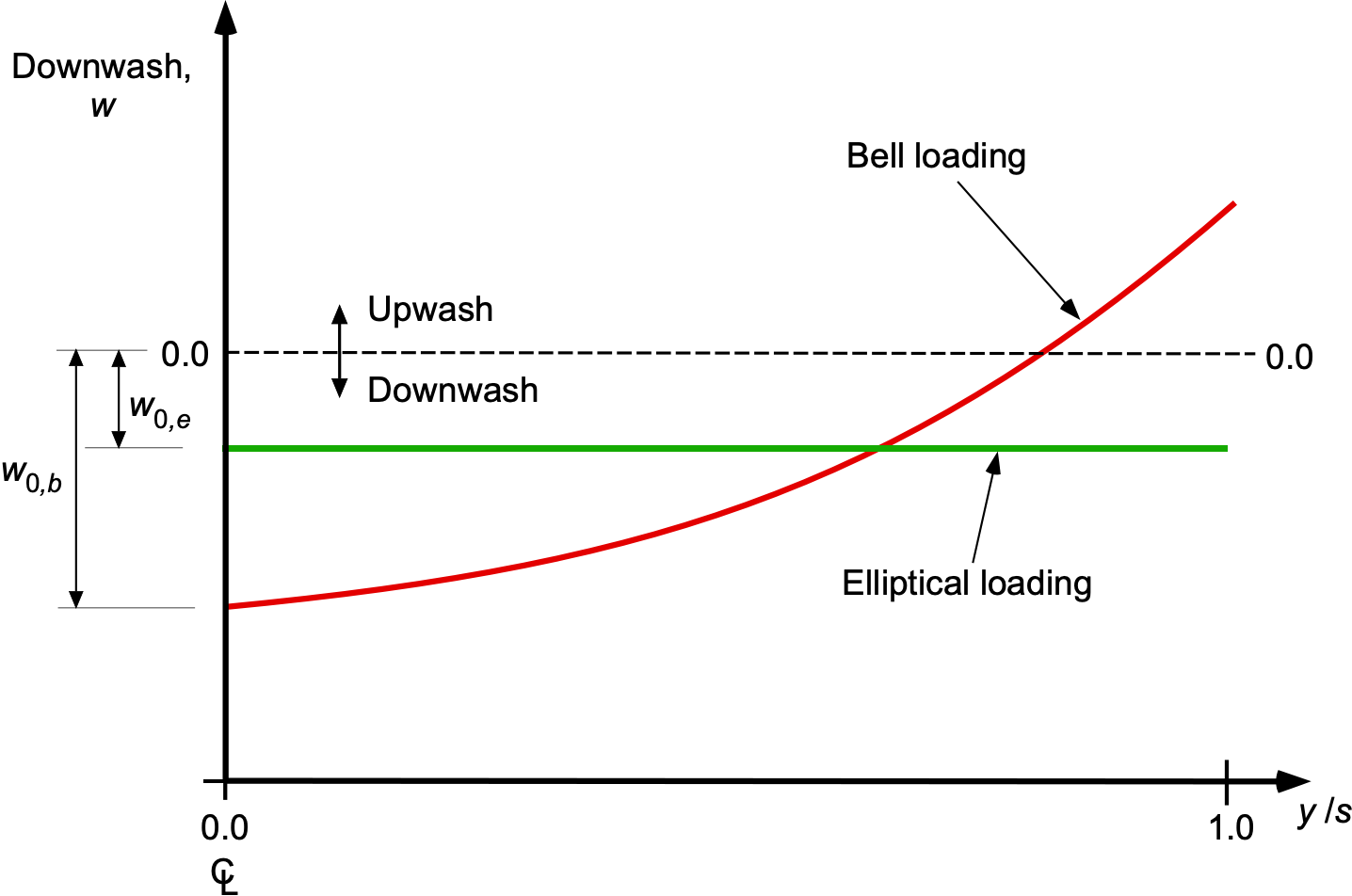
Wing Lift
The lift on a wing, according to the Kutta-Joukowsky theorem, is given by
(171) 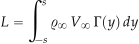
The standard lifting line transformation that can be used, where  . In this case, the total wing lift is
(172) 
Substituting  for the elliptical loading gives
(173) 
In terms of the coordinate, the bell-shaped spanwise circulation distribution is given by
(174) 
Substituting this distribution into the lift equation gives
(175) 
If the elliptically loaded and bell-loaded wings produce the same lift, then  , so their peak values of circulation are related by
(176) 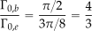
Induced Drag Distribution
Because of the low geometric angles and upwash generated by the bell-shaped spanwise loading over the tip regions, they produce a forward-acting lift vector, resulting in negative induced drag. The downwash has been previously derived in Eq. 170, so the form of the local induced drag coefficient follows directly. For the elliptical loading, then
(177) 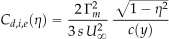
where  , and for the bell loading
(178) 
where is the local wing chord. As shown in the figure below, for which a rectangular planform with = constant is assumed, the induced drag becomes negative outboard of  = 0.707. Notice that when using Eq. 176, then
(179) 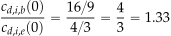
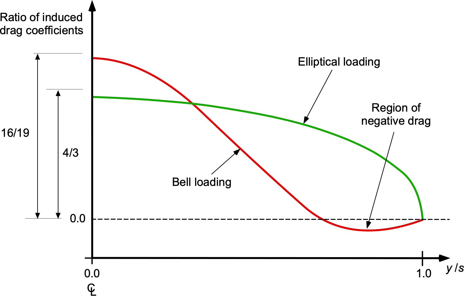
It is the forward-acting lift vector at the wing tips, as shown for the sectional level in the figure below, that proves necessary to give stability and control to a flying wing. However, the net drag on the wing is still positive for a given span and aspect ratio, the bell-shaped form of wing loading producing higher overall induced drag compared to a wing with the elliptical loading, i.e., the spanwise loading factor, , will be greater than zero, as will be shown later.
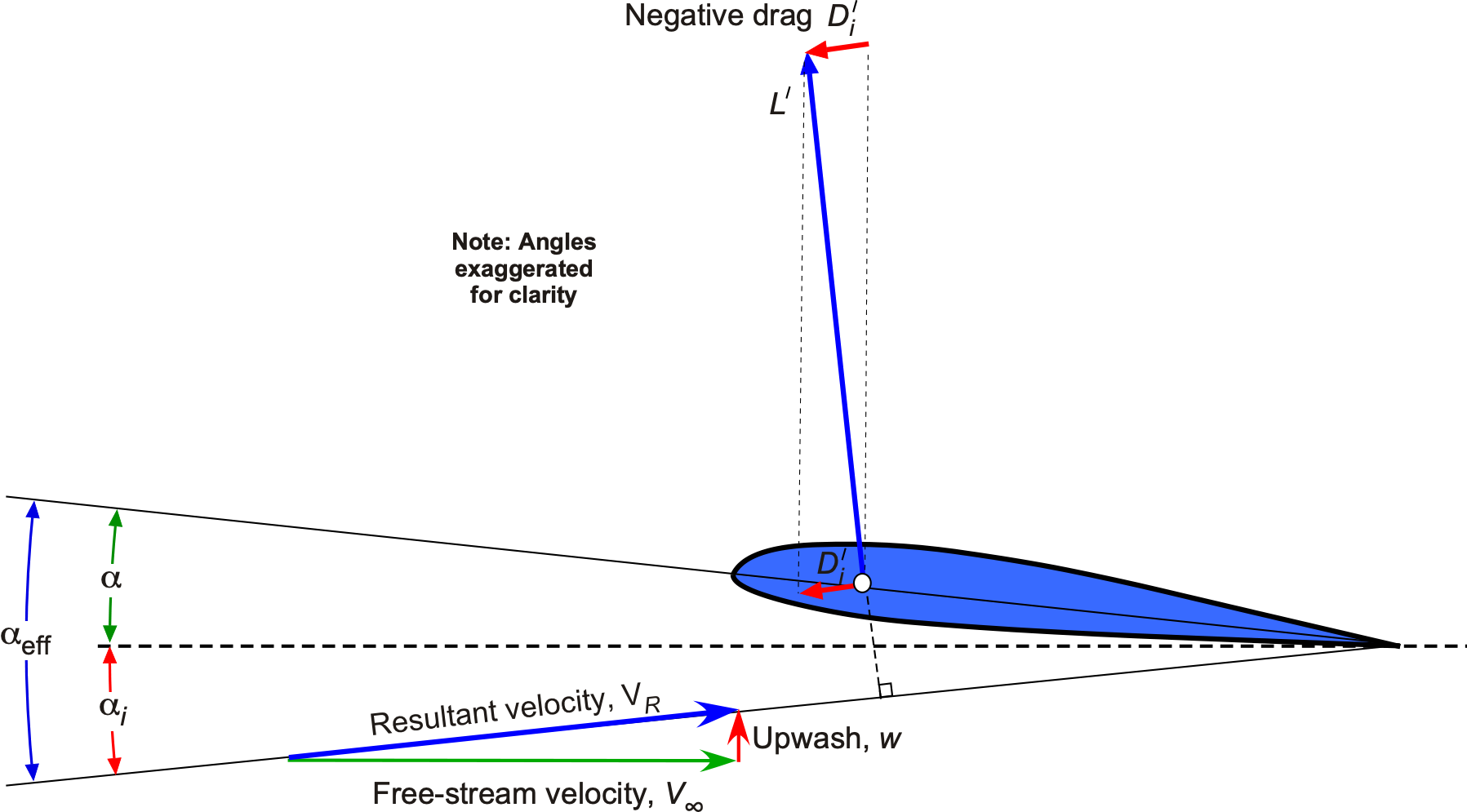
Lift Coefficient Distribution
For a rectangular planform where the chord and section lift-curve slope are constant, the local section lift coefficient is directly proportional to the bound circulation. Consequently, the spanwise lift-coefficient distributions corresponding to the two loadings are
(180) 
Normalizing by the mid-span value gives the purely geometric forms as
(181) 
or
(182) 
where . Therefore, the bell-shaped loading will generally have the lower values at the wing tips than the elliptical loading for the same wing planform. This distribution gives a flying wing good stall qualities because the inboard sections stall first, the wing maintaining its directional stability while the flaperons remain effective.
Wing Twist Distribution
It is necessary to use planform shape and nonuniform wing twist to produce the bell-shaped form of spanwise loading, with significant nose-down twist being needed over the outer span. The general form of the nonlinear twist needed to create the bell-shaped loading is
(183) 
where  and
and  depend on the details of the wing planform as well as the airfoil section as it affects the zero-lift angle of attack.
The approach to finding the needed twist on the wing to achieve the bell-shaped loading is straightforward. With the bell circulation distribution, then
(184) 
where  . If a rectangular wing of unit chord is assumed, then
  . The section lift coefficient is
(185) 
In terms of section angles, then
(186) 
where  is the geometric angle of attack or pitch measured relative to the reference or datum,
  . Therefore, the needed twist distribution can be expressed as
(187) 
Using  = 2/rad for the sectional lift curve slope, then
(188) 
For the bell-shaped spanwise loading, then  , so the needed twist is
(189) 
where the lift coefficient, , can be interpreted as the design lift coefficient for the wing, such as in cruise flight. This equation represents the unique geometric twist that creates both the bell spanwise loading and its unique downwash distribution for a wing of constant chord, as illustrated in the figure below. If the wing has taper and/or camber, which is typical, the lifting-line problem and the needed spanwise twist can be solved numerically; however, the fundamental approach remains the same.
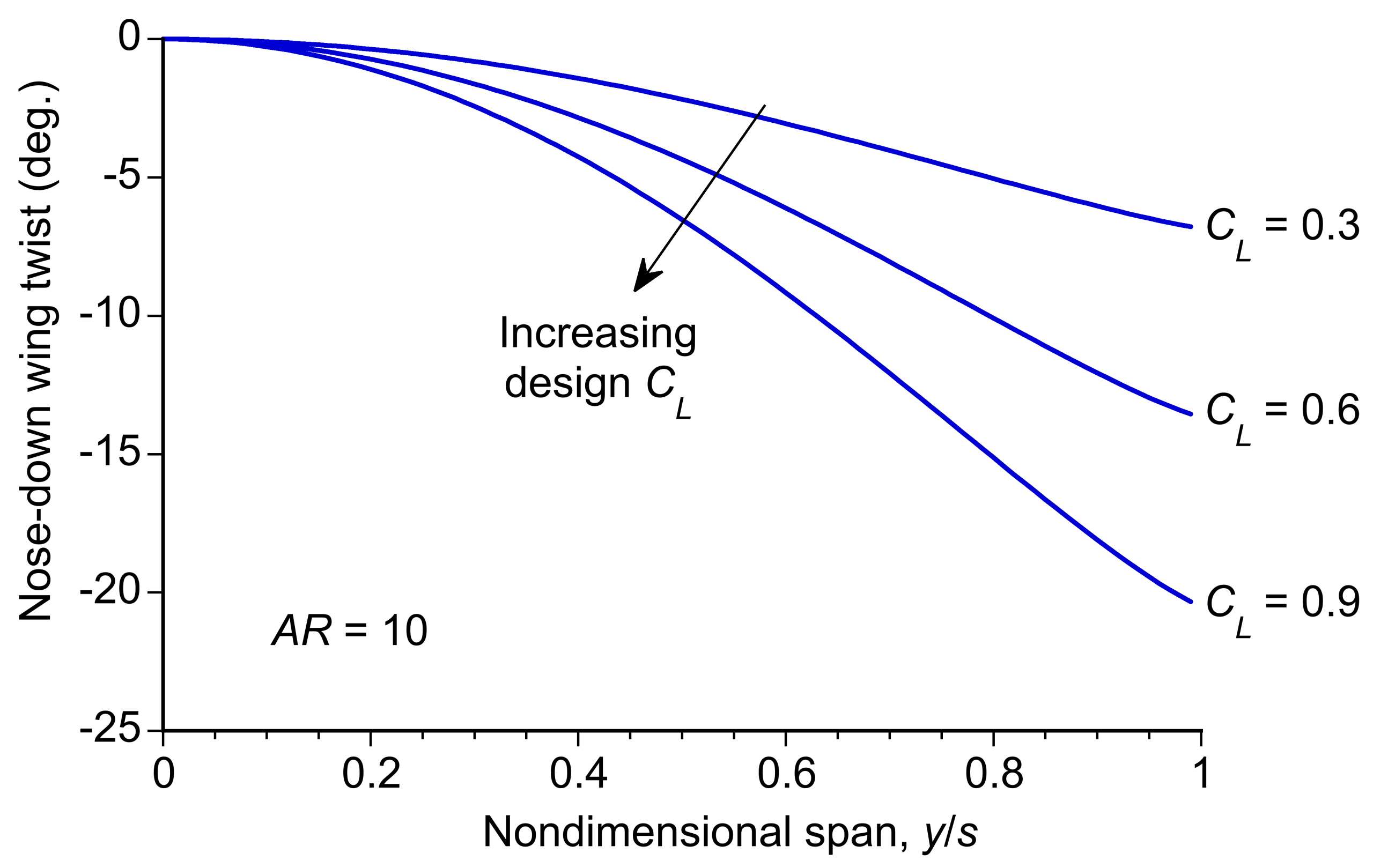
Wing Bending Moments
In his 1933 paper, Prandtl minimized the integral of the square of the bending moment (an energy proxy) while maintaining a constant total lift. The key argument in the use of other than an elliptical wing loading is to minimize wing bending and hence reduce wing weight, although at the expense of some loss of aerodynamic efficiency. Prandtl remarked in his paper that one may “regard the integrated bending moment as a measure of spar weight.” A reasonable assumption, therefore, is that wing weight is proportional to the characteristic wing bending moment. Later, R.T. Jones[10] made similar arguments with similar outcomes.
The wing root bending moment is obtained by integrating the aerodynamic loading from the tips to the root, i.e., using
(190) 
For the elliptical loading, where  , then
(191) 
For the bell-shaped loading, where  , then
(192) 
To produce the same total lift, the peak circulation of the bell-shaped loading must be  , as shown in the previous figure. Substituting these relationships gives
(193) 
so the ratio of the bending moments is
(194) 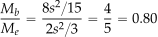
This result indicates that the bell-shaped loading gives a lower spanwise bending moment overall and a 20% reduction in the root bending moment compared to the elliptical loading, for the same total wing lift, as illustrated in the figure below. This outcome has significant implications for the design of a wing with a bell-shaped spanwise loading because it can be lighter than if it had the elliptical loading with some increase in induced drag for the same span.
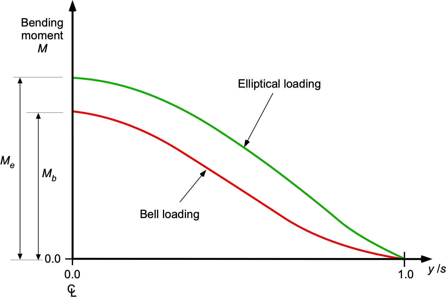
Total Induced Drag
The induced drag for a wing with the bell-shaped spanwise loading distribution can now be determined. For the elliptical loading, where , then
(195) 
For the bell-shaped loading, where , the induced drag is
(196) 
To ensure equal total lift, the peak circulation values must be scaled using . Substituting gives
(197) 
Therefore, the ratio of induced drag values is
(198) 
Because, in general, the induced drag coefficient is
(199) 
and because  = 0 for the elliptic loading, then it can be concluded that
  = 1.219. This result shows that the bell-shaped spanwise loading produces 21.9% more induced drag than the elliptical distribution, keeping in mind that this is for the same total lift and wing span. This is an expected outcome based on the significant spanwise deviations of the bell-shaped loading from the elliptical ideal.
Design Application
The primary reason for using a bell-shaped spanwise loading is that for flying wings or other tailless airplane configurations, the upwash at the wing tips helps give yaw stability and eliminates adverse yaw effects. Ideally, this goal should be achieved without either aerodynamic or structural weight penalty. Therefore, a final step is to determine a new wing span with a bell-shaped spanwise loading that yields the same structural root bending moment as the elliptical loading, while maintaining the same total wing lift, wing area, and without as much of an induced drag penalty.
From Eq. 190, it is apparent that the wing root bending moment scales with the square of the semi-span, i.e.,  , or equivalently
  . From the previous results, it was shown that the root bending moment for the bell-shaped loading is 80% of that for the elliptical loading, i.e.,
  . Therefore, the span of a bell-loaded wing that produces the same root bending moment as an elliptically loaded wing can be increased by
(200) 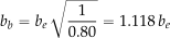
which corresponds to an 11.8% increase in wing span. Consequently, the wing aspect ratios are related by
(201) 
if the wing area is held constant. The aspect ratio scales with the square of the span, so for the bell-shaped loading, then
(202) 
and for an 11.8% increase is span, then
(203) 
Therefore, the aspect ratio increases by 25% with the wing area being held constant. In this case, the induced drag coefficients, which are both for the bell-shaped loading, will be related using Eq. 199 by
(204) 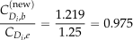
This result shows that by adopting a bell-shaped spanwise loading and not allowing the structural root bending moment to increase over that obtained with the elliptical loading, the wing span can be increased by 11.8% (for the same wing area), resulting in a 25% increase in aspect ratio and a 2.5% reduction in induced drag. It will be apparent that, in general, then
(205) 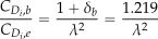
as shown in the plot below. Such is the powerful advantage of the aspect ratio as a means of offsetting less-than-ideal spanwise loading distributions on a wing.
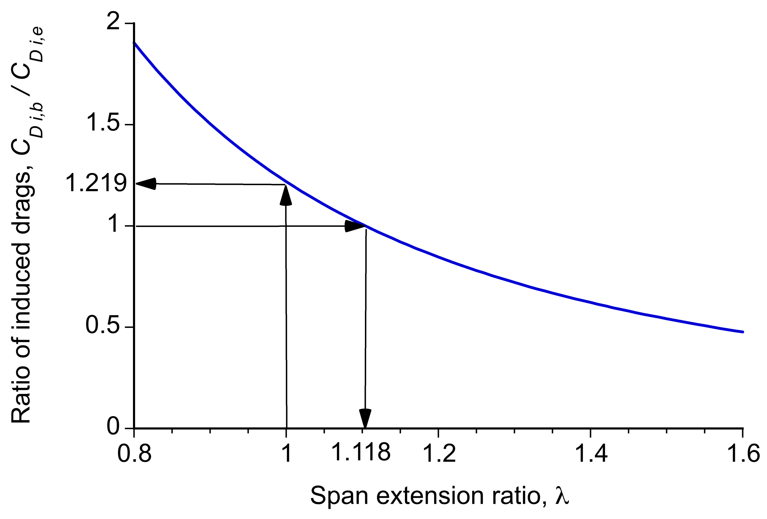
This is an interesting and potentially important result in airplane design, not just limited to flying wings. When geometric span alone constrains the wing design, the elliptical spanwise loading remains optimal. However, the main reason for using an alternative spanwise loading, in this case, the bell-shaped loading, is the upwash it produces at the wing tips, which inclines the lift vectors forward rather than aft, as previously described. This condition produces the directional stability on a tailless flying wing and also gives a desirable proverse yaw effects with the application of flaperons or ailerons.
This characteristic is crucial for the success of flying wings, and is the primary advantage of designing the wing to give a bell-shaped spanwise loading, despite the penalty of a higher induced drag factor, , of 0.219. But, if the wing span is not a design constraint, then the induced drag penalty from the use of a bell-shaped spanwise loading, or any other non-ideal loading for that matter, can be offset by using a wing of modestly higher span and aspect ratio. The consideration of increased wing weight, however, still remains an issue.
It has been demonstrated that the root bending moment is proportional to the product of lift and span. However, a 12% increase in span incurs no net wing weight penalty with the bell-shaped loading and reduces the induced drag as a result of the higher aspect ratio. Further increasing the wing span, say by 20%, increases the bending moment by the same fraction for the same wing lift. The weight of a wing grows roughly with the cube of its span, an outcome of the square-cube law. Taking also the lower inboard bending moment achieved with the bell loading (i.e.,  ), a first-order wing weight estimate is
(206) 
Even after benefiting from the bell loading’s lower inboard bending moment, when the span grows too much, the cubic term in Eq. 206 produces a 40% increase in wing weight. Therefore, when both drag and weight are considered, the optimum wing design typically involves using only enough extra wing span to make the structural cost aerodynamically worthwhile.
Introduction to Lifting Surface Theory
The progression from lifting line theory to lifting surface theory and eventually to incorporating thickness represents a series of refinements in aerodynamic modeling using vortex methods. Each step increases the model’s fidelity by including additional aspects of three-dimensional flow around finite wings. Lifting line theory is the simplest of these models, in which the wing is represented as a single line of bound circulation located at the quarter-chord along the span. While straightforward and analytically elegant, lifting line theory does not account for chordwise loadings or the presence of wing thickness and camber, limiting its applicability to more complex wing geometries, including those with sweep or non-planar geometries.
Lifting surface theory, also known as the vortex lattice or vortex panel method, extends this framework by treating the wing as a surface. The circulation is now distributed across both the span and the chord, denoted by  , allowing for a more realistic spatial representation of aerodynamic loading. As shown in the figure below, this approach utilizes distributed vortex sheets in the form of quadrilateral panels to model both spanwise and chordwise variations in lift.
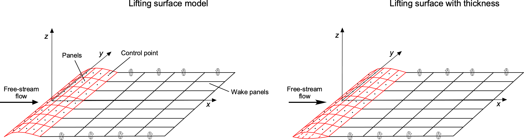
The induced downwash at a control point at  is obtained from the net effect of all vortex elements using
(207) 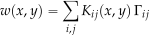
where  is an influence coefficient matrix associated with the unit-strength vortex element at
  . Each entry is a scalar representing the vertical velocity induced at the control point by a unit-strength vortex element at , and the matrix is assembled from these scalar entries.
The actual strengths of the vortex elements are then solved for by satisfying the flow tangency (the no-penetration condition) at control points located at the centroids of each panel. This condition is expressed as
(208) 
where  is the net velocity at the surface and
  is the local unit normal vector. The net velocity is composed of the freestream and induced components, i.e.,
(209) 
Substituting into the boundary condition gives
(210) 
In many practical implementations, such as the classical vortex lattice method, the surface is assumed to lie approximately in the  – plane, and the unit normal vector is taken to point in the
  direction. Therefore, the boundary condition reduces to a scalar equation involving the vertical component of velocity, i.e.,
(211) 
For small angles, the boundary condition is simplified to
(212) 
where  is the local induced angle of attack resulting from the downwash. This relation is based on the small-angle approximation and the linear relationship
(213) 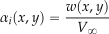
Therefore, the equations to be solved are
(214) 
Solving this set of linear simultaneous equations yields the vortex strengths  over the lifting surface, from which the spanwise and chordwise loading distributions can then be determined. Solving the linear system typically involves assembling the influence matrix and applying boundary conditions to determine using matrix inversion or iterative solution methods.
Lifting surface theory significantly improves the fidelity of aerodynamic predictions, particularly for wings with moderate or low aspect ratios, but it continues to assume a thin airfoil shape. However, as also illustrated in the figure above, the lifting surface model can be extended to include wing thickness and camber. Wing thickness introduces an additional layer of aerodynamic complexity because a wing with finite thickness alters the chordwise and spanwise pressure distributions, and hence the lift distribution and induced drag. Alternatively, source distributions can be added to the thin vortex sheet representation to model thickness effects. In this case, the total potential is then expressed as
(215) 
Here,  represents the bound vortex strength, as before, and
  denotes the distributed source strength over the surface . The quantity is the distance from the field point to the source point, defined as
(216) 
Such lifting surface models, with thickness and camber, form the foundation of many modern aerodynamic “panel methods” for analyzing arbitrary aircraft configurations. While classical lifting surface theory models the wing as a distribution of bound vortices, modern panel methods incorporate vortex and source distributions to model thickness and camber effects.
Summary & Closure
The lifting line theory provides a foundational framework for analyzing the aerodynamic behavior of finite wings. By modeling the wing as a spanwise distribution of bound circulation and accounting for the induced downwash generated by the trailing vortex system, the theory allows for estimating essential aerodynamic quantities such as the lift distribution and induced drag Although the theory relies on simplifying assumptions, including high aspect ratio, small angles of attack, and inviscid, incompressible flow, it represents the essential physics governing three-dimensional wing aerodynamics with reasonable accuracy. It remains a core analytical tool in aircraft design because of its simplicity, analytical tractability, and predictive capability.
For multiple lifting surfaces, such as biplanes, the theory must be extended to account for aerodynamic interference between the wings. Biplane theory models each wing as a lifting line and includes the mutual downwash that one wing induces on the other. This coupling modifies the local angle of attack and alters the spanwise circulation distribution, resulting in increased induced drag compared to an isolated wing. The aerodynamic penalty is commonly expressed through an interference factor that quantifies the degradation in performance relative to a monoplane of equivalent span and total lift. Parameters such as gap, stagger, decalage, and chord ratio significantly influence the interference and, therefore, affect the overall efficiency of the wing configuration.
To better represent three-dimensional effects and more general wing geometries, the lifting line theory can be extended to a lifting surface theory, which treats the wing as a two-dimensional surface rather than a line. This approach discretizes the wing into a grid of panels or vortex elements, allowing for the simultaneous resolution of both spanwise and chordwise variations in vorticity. Lifting surface methods, such as vortex lattice models, account for non-uniform chord, sweep, taper, and airfoil thickness because they enforce the flow tangency condition across the entire wing surface. These models are intermediate between simple analytical theories and full computational fluid dynamics (CFD) simulations.
5-Question Self-Assessment Quickquiz
For Further Thought or Discussion
- How might the assumptions used in lifting line theory (inviscid, incompressible flow) affect the quality of predictions of actual wings?
- Why does the elliptical circulation distribution minimize induced drag, and what are the practical challenges in achieving it for non-elliptic wing planforms?
- How does increasing a wing’s aspect ratio improve aerodynamic efficiency but introduce structural and design challenges?
- How do wings with rectangular or linearly tapered shapes deviate from elliptic loading, and how does this impact induced drag and overall wing performance?
- Why is the lifting line theory inapplicable in supersonic flows, and how are these issues addressed in modern aerodynamics?
- How might winglets be modeled within the framework of the lifting line theory? What types of modifications, if any, may be required?
- How does wing twist affect wing performance and allow for loading optimization under specific flight conditions?
- What are some examples of aircraft that achieve near-elliptic wing loading?
- How is the lifting line theory or its derivatives applied in other contexts, such as rotor blades, wind turbines, or hydrofoils?
Other Useful Online Resources
To understand more about the aerodynamics of finite wings and wing theory, explore some of these online resources:”
- Finite Wings – Lifting Line Theory” from the Postcard Professor.”Prandtl’s Lifting Line Theory” by Professor Sid G.
- “Lifting Line Theory” by Professor Lakshmi Sankar at GaTech.
- Lecture notes from MIT OpenCourseWare introduces Prandtl’s lifting line theory, including geometry and fundamental definitions.
- A comprehensive overview of lifting line theory, including its principles, derivation, and applications.
- An explanation of Prandtl’s lifting line theory, focusing on three-dimensional potential flow, provided by the University of Cambridge.
- Lecture notes from Stanford University discussing finite wing theory and related details, including lifting line theory.
- An educational website offering resources on various aerodynamics topics, including lifting line theory.
- A GitHub repository containing Python code implementing Prandtl’s lifting line theory for aerodynamic analysis.
- Lecture notes from MIT OpenCourseWare focusing on force calculations within lifting line theory.
- A tutorial example providing practical insights into applying lifting line theory.
- Lecture notes offering a detailed explanation of lifting line theory concepts.
- A collection of MATLAB scripts and functions implementing lifting line theory for aerodynamic analysis.
- The addition of a winglet will cause the tip vortex to form at the tip of the winglet. ↵
- Prandtl's original publication on the lifting-line theory was "Über Tragflügeltheorie" ("On Wing Theory"), which was published in 1904 in the proceedings of the Third International Congress of Mathematicians in Heidelberg, Germany. This paper introduced the fundamental ideas of the lifting-line theory. ↵
- Hermann Glauert was a British aerodynamicist and a pioneer in theoretical aerodynamics.
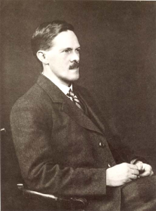 He worked at the Royal Aircraft Establishment (RAE) and is best known for his contributions to thin airfoil theory and lifting line theory. His influential book, "The Elements of Aerofoil and Airscrew Theory," remains a classic. ↵
 - Glauert systematically presented this theory in his 1926 book The Elements of Aerofoil and Airscrew Theory. ↵
- This transformation is analogous to the one used in the thin airfoil theory. ↵
- There is also a biplane wing theory, which is considered later in this chapter. ↵
- R. T. Jones, "The Spanwise Distribution of Lift for Minimum Induced Drag of Wings Having a Given Lift and a Given Bending Moment," NACA TN-2249, 1950. ↵
- Proverse yaw occurs because the increased lift and reduced drag on the down-going aileron facilitated by the upwash, eliminates the adverse yaw effects that would typically occur with a conventional airplane. ↵
- Prandtl, L., "Über die Tragfähigkeit der Flügel (On the Lift of Wings)," Zeitschrift für Flugtechnik und Motorluftschiffahrt, 1933. See also: "Ludwig Prandtl’s 1933 Paper Concerning Wings for Minimum Induced Drag, Translation and Commentary," AIAA 2020-0644. AIAA Scitech 2020 Forum. January 2020. ↵
- Jones, R. T., "The Spanwise Distribution of Lift for Minimum Induced Drag of Wings Having a Given Lift and a Given Bending Moment," NACA Technical Note 2249, Dec. 1950. ↵