Worked Examples: Airplane, Rocket, & Spacecraft Performance

J. Gordon Leishman

69 Worked Examples: Airplane, Rocket, & Spacecraft Performance

These worked examples have been fielded as homework problems or exam questions.

Worked Example #1

A propeller-driven airplane has a fuel flow ${\overbigdot{W}_f}$ to the engines of the form

$\frac{dW_f}{dt} = {\overbigdot{W}_f} = c_{b} \left( A V_{\infty}^3 + \frac{B}{V_{\infty}} \right)$

where ${\overbigdot{W}_f}$ is the weight of fuel burned per unit time, $V_{\infty}$ is the true airspeed, $c_b$ is the brake specific fuel consumption. The values of $A$ and $B$ depend on the characteristics of the airplane, its weight, and the density altitude at which it is flying, i.e.,

$A = \frac{1}{2} \varrho_{\infty} S C_{D_{0}} \mbox{~~~~and~~~~} B = \frac{2 W^2}{\varrho_{\infty} S (\pi \, AR e)}$

Based on this fuel flow equation, show that the airspeed for the best endurance for the airplane will be obtained when the true airspeed is

$V_{\infty} = V_x = \left(\frac{B}{3A}\right)^{1/4}$

and the corresponding airspeed for the best range for the airplane will be obtained when the true airspeed is

$V_{\infty} = V_y = \left(\frac{B}{A}\right)^{1/4}$

Explain the operational significance of flying at $V_x$ and $V_y$ , and give an example of a flight profile (or a part of one) when such airspeeds might be specifically used.

The first term in the fuel flow equation is the contribution from the profile/parasitic (non-lifting) part of the drag, which grows with the cube of the airspeed. The second part is the contribution from the induced drag, which is inversely proportional to airspeed. Starting from

$\frac{dW_f}{dt} = {{\overbigdot{W}_f}} = c_b\left( A V_{\infty}^3 + \frac{B}{V_{\infty}} \right)$

then the lowest fuel burn (hence maximum flight endurance) can be determined by finding when ${\overbigdot{W}_f}$ is a minimum. Differentiating the fuel flow equation with respect to $V_{\infty}$ gives

$\frac{d{\overbigdot{W}_f}}{dV_{\infty}} = c_b \left( 3 A V_{\infty}^2 - \frac{B}{V_{\infty}^2} \right)$

which is zero for a minimum, i.e.,

$3 A V_{\infty}^2 - \frac{B}{V_{\infty}^2} = 0$

and so

$V_{\infty} = V_x = \left( \frac{B}{3A} \right)^{1/4}$

The best range is obtained when the ratio ${\overbigdot{W}_f}/V_{\infty}$ is a minimum. In this case

$\frac{{\overbigdot{W}_f}}{V_{\infty}} = c_b \left( A V_{\infty}^2 + \frac{B}{V_{\infty}^2} \right)$

so that

$\frac{d({\overbigdot{W}_f}/V_{\infty})}{dV_{\infty}} = c_b \left( 2 A V_{\infty} - 2\frac{B}{V_{\infty}^3} \right)$

which is zero for a minimum, i.e.,

$2 A V_{\infty} - \frac{2B}{V_{\infty}^3} = 0$

and so

$V_{\infty} = V_y = \left( \frac{B}{A} \right)^{1/4}$

There are a variety of missions where flight at the speed for the best range and best endurance are essential. For example, a long-range ferry mission of the airplane (say, over water) might need the airplane to be flown at or near its airspeed for the best range, even though this airspeed is typically lower than the best cruise speed of the airplane. Likewise, flight at an airspeed for best endurance might be needed for a reconnaissance mission where the airplane might have to fly at or near a particular location for an extended period.

Worked Example #2

Starting from the steady, level-flight flight assumption of $L = W$ and $T = D$ , and assuming the engine thrust specific fuel consumption TSFC ( $c_t$ ) is constant, then show that for a jet-propelled airplane flying at a constant altitude that the fuel flow to the engines in terms of weight of fuel burned per unit time ${\overbigdot{W}_f}$ can be expressed in the form

${{\overbigdot{W}_f}} = A V_{\infty}^2 + \frac{B}{V_{\infty}^2}$

where you should evaluate $A$ and $B$ in terms of the the wing area, $S$ , wing aspect ratio, $A\!R$ , flight weight, $W$ , parasitic drag coefficient & $C_{D_{0}}$ , Oswald’s efficiency factor, $e$ , engine TSFC, $c_t$ .

The standard formula gives the lift $L$ on the airplane.

$L = \frac{1}{2} \varrho_{\infty} \, V_{\infty}^2 \, S \, C_L$

which is equal to weight $W$ . The drag $D$ on the airplane is

$D = \frac{1}{2} \varrho_{\infty} V_{\infty}^2 S C_D$

where the drag coefficient $C_D$ is given by

$C_D = C_{D_{0}} + C_{D_{i}} = C_{D_{0}} + \frac{{C_L}^2}{\pi \, AR e}$

i.e., the sum of non-lifting and lifting (induced) parts. $A\!R$ is the wing’s aspect ratio, and $e$ is Oswald’s efficiency factor. Using the equation for lift (as well as the assumption that $L = W$ ), the lift coefficient is

$C_L = \frac{2 L}{\varrho_{\infty} V_{\infty}^2 S} = \frac{2 W}{\varrho_{\infty} V_{\infty}^2 S}$

Also, because the thrust $T$ equals drag, then

$T = \frac{1}{2} \varrho_{\infty} V_{\infty}^2 S C_{D_{0}} + \frac{1}{2} \varrho_{\infty} V_{\infty}^2 S \left( \frac{2 W}{\varrho_{\infty} V_{\infty}^2 S} \right)^2 \left( \frac{1}{\pi \, AR e} \right)$

and after rearrangement, then

$T = \frac{1}{2} \varrho_{\infty} V_{\infty}^2 S C_{D_{0}} + \frac{2 W^2}{\varrho_{\infty} V_{\infty}^2 S (\pi \, AR e)}$

For a jet engine, the fuel burn rate ${\overbigdot{W}_f}$ will be the product of the thrust and the thrust-specific fuel consumption, i.e.,

$\frac{d W_f}{dt} = {\overbigdot{W}_f} = T c_t$

Substituting for $T$ gives

${\overbigdot{W}_f} = \frac{1}{2} \varrho_{\infty} V_{\infty}^2 S c_t C_{D_{0}} + \frac{2 c_t W^2}{\varrho_{\infty} V_{\infty}^2 S (\pi \, AR e)}$

or

${\overbigdot{W}_f} = \left( \frac{1}{2} \varrho_{\infty} S c_t C_{D_{0}} \right) V_{\infty}^2 + \left( \frac{2 c_t W^2}{\varrho_{\infty} S (\pi \, AR e)} \right) \frac{1}{V_{\infty}^2}$

which is of the form

${\overbigdot{W}_f} = A V_{\infty}^2 + \frac{B}{V_{\infty}^2}$

where

$A = \frac{1}{2} \varrho_{\infty} S c_t C_{D_{0}}$

and

$B = \frac{2 c_t W^2}{\varrho_{\infty} S (\pi \, AR e)}$

Both constants are based on the stated assumptions of all the values involved for a constant weight $W$ and altitude, i.e., $\varrho_{\infty}$ = constant.

Worked Example #3

Using the fuel flow equation from the previous worked example, i.e.,

${{\overbigdot{W}_f}} = \frac{d W_f}{dt} = A V_{\infty}^2 + \frac{B}{V_{\infty}^2}$

show that the airspeed for the best endurance for a jet airplane will be obtained when

$V_{\infty} = V_x = \left(\frac{B}{A}\right)^{1/4}$

In this problem, we are asked to start from

$\frac{d W_f}{dt} = {\overbigdot{W}_f} = A V_{\infty}^2 + \frac{B}{V_{\infty}^2}$

The lowest fuel burn (hence maximum flight endurance) can be determined by differentiating the fuel flow equation with respect to $V_{\infty}$ , i.e.,

$\frac{d{\overbigdot{W}_f}}{dV_{\infty}} = 2 A V_{\infty} - \frac{2 B}{V_{\infty}^3}$

which is zero for a minimum, i.e.,

$2 A V_{\infty} - \frac{2B}{V_{\infty}^3} = 0$

and so

$V_{\infty} = V_x = \left( \frac{B}{A} \right)^{1/4}$

where

$A = \frac{1}{2} \varrho_{\infty} S c_t C_{D_{0}}$

and

$B = \frac{2 c_t W^2}{\varrho_{\infty} S (\pi \, AR e)}$

So $V_x$ would be the airspeed at which the airplane can fly with minimum fuel flow. This speed depends on the airplane’s weight and altitude.

Worked Example #4

An ERAU Cessna 172 Skyhawk airplane is flying along at an estimated in-flight weight of 2,100 lb and an airspeed of 120 knots at 2,000 ft where the air density is 0.00216 slugs/ft ${^3}$ . The student pilot is flying solo on a long cross-country flight. When flying over Jacksonville airport on the way back to ERAU (125 nautical miles left to fly), the pilot notices from the fuel gauge that only 8 gallons of usable AVGAS fuel remain in the tanks. Assume that the airplane’s weight for this analysis is the initial in-flight weight minus half the remaining fuel weight. Assume also that AVGAS fuel weighs 6.0 lb per gallon. The engineering characteristics of the airplane are given below:

Wing span, $b$ = 36 ft
Wing area, $S$ = 174 ft $^2$
Non-lifting drag coefficient, $C_{D_{0}}$ = 0.02
Average propeller efficiency, $\eta_p$ = 0.85
Oswald’s efficiency factor, $e$ = 0.81
Engine BSFC, $c_b$ = 0.45 lb hp $^{-1}$ hr $^{-1}$

Calculate the following:
(a) The operating lift coefficient of the wing, $C_L$ .
(b) The induced drag coefficient, $C_{D_{i}}$ and the total drag coefficient, $C_D$ .
(c) The lift-to-drag ratio of the airplane.
(d) The propeller thrust and engine power (in hp) required for the airplane to fly.
(e) The fuel flow in gallons per hour. Will the pilot make it back to ERAU using the remaining fuel?

We are told to assume that the airplane’s weight for this analysis is the initial in-flight weight, say $W_0$ , less half the remaining fuel weight. We have only 8 gallons of AVGAS fuel, and we are told to assume AVGAS weighs 6.0 lb per gallon, so $W_f$ = 48 lb of fuel. Therefore, the weight to perform the analysis is

$W = W_0 - \frac{W_f}{2} = 2,100 - \frac{48.0}{2} = 2, 076~\mbox{lb}$

An airspeed of 120 kts is equivalent to 120 $\times$ 1.688 = 202.54 ft/s = $V_{\infty}$ .

(a) The operating lift coefficient of the wing, $C_L$ , is

$C_L = \frac{2W}{\varrho V^2 S} = \frac{2 \times 2,076}{0.00216 \times 202.54^2 \times 174.0} = 0.269$

(b) To find the induced drag coefficient, we need the aspect ratio of the wing, $A\!R$ , i.e.,

$A\!R = \frac{b^2}{S} = \frac{(36.0)^2}{174.0} = 7.45$

The induced drag coefficient $C_{D_{i}}$ will be

$C_{D_{i}} = \frac{{C_L}^2}{\pi \, AR e} = \frac{0.269^2}{\pi \times 7.45 \times 0.81} = 0.00382$

The total drag coefficient, $C_D$ , is

$C_D = C_{D_0} + C_{D_i} = C_{D_0} + \frac{{C_L}^2}{\pi \, AR e} = 0.02 + 0.00382 = 0.02382$

(c) The lift-to-drag ratio of the airplane at the given conditions of flight is

$\frac{L}{D} = \frac{C_L}{C_D} = \frac{0.269}{0.02382} = 11.3$

(d) The thrust $T$ from the propeller required for the airplane to fly is

$\frac{W}{C_L/C_D} = \frac{2,076}{11.3} = 183.7~\mbox{lb}$

The power required for flight $P_{\rm req}$ will be

$P_{\rm req} = \frac{ T \, V_{\infty} }{\eta_p} = \frac{183.7 \times 202.54}{0.85 \times 550} = 79.6~\mbox{hp}$

where the conversion factor 550 has been used to convert the base USC units to standard units of horsepower (hp).

(e) The fuel flow now follows directly, i.e.,

$\frac{d W_f}{dt} = {\overbigdot{W}_f} = P_{\rm req} \, c_b = 79.6 \times 0.45 = 35.8~\mbox{lb hr$^{-1}$}$

So, the airplane is using about 6 gallons per hour.

(f) The time to burn off all of the relatively small amount of available fuel is

$\mbox{Time} = T_i = \frac{48.0}{35.8} = 1.341~\mbox{hrs}$

So, the potential approximate range of the airplane is

$\mbox{Range} = R = 1.341 \times 120 \approx 160~\mbox{nautical~miles}$

In conclusion, the airplane has enough fuel to return to ERAU. But, in practice, the FAA requires a minimum fuel reserve of 30 minutes of flight time (visual rules) and 45 minutes of flight time (instrument rules), so legally, the student pilot is probably going to have to land and pick up more fuel before completing the final leg back to ERAU.

Worked Example #5

Consider a small jet-powered airplane with an initial in-flight weight of 21,000 lb flying in unaccelerated level flight at an airspeed of 250 knots where the air density is 0.0015 slugs/ft ${^3}$ . The airplane weighs 850 lb of usable fuel remaining in its tanks. The airplane’s wing span is 48.0 ft, and the wing panels have a trapezoidal shape with a root chord $c_r$ = 9 ft and a tip chord $c_t$ = 4 ft. The other characteristics of the airplane are: Non-lifting drag coefficient, $C_{D_{0}}$ = 0.02; Oswald’s efficiency factor, $e$ = 0.81; Engine TSFC = $c_t$ = 0.5 lb lb^-1 hr^-1. Assume for the following analysis that the airplane’s weight from fuel burning is the initial weight minus half the remaining fuel weight. Calculate the following:

(a) The operating lift coefficient of the wing, $C_L$ .
(b) The induced drag coefficient, $C_{D_{i}}$ and the total drag coefficient, $C_D$ .
(c) The lift-to-drag ratio of the airplane in the given flight conditions.
(d) The thrust $T$ required from the engines for the airplane to fly.
(e) The approximate maximum potential remaining flight range of the airplane.
(f) The approximate flight time to reach the remaining flight range.

We need initial information, including the wing area and aspect ratio, as well as the weight at which to run the calculations. Calculating the area of the wing gives

$S = b\frac{(c_r + c_t)}{2} = 48.0 \left( \frac{9.0 + 4.0}{2} \right) = 312.0~\mbox{ft}^2$

The aspect ratio can be calculated using

$A\!R = \frac{b^2}{S} = \frac{(48.0)^2}{312.0} = 7.38$

We are told to use the weight of the airplane at a point which is its initial weight minus half the remaining fuel weight, so

$W = W_0 - \frac{W_f}{2} = 21,000 - \frac{850.0}{2} = 20,575~\mbox{lb}$

(a) An airspeed of 250 kts is equal to 422 ft/s. The operating lift coefficient of the wing, $C_L$ , is

$C_L = \frac{2W}{\varrho V^2 S} = \frac{2 (20,575)}{0.0015 (422.0)^2 312.0} = 0.494$

(b) The total drag coefficient, $C_D$ , is

$C_D = C_{D_0} + C_{D_i} = C_{D_0} + \frac{{C_L}^2}{\pi \, AR \, e} = 0.02 + \frac{0.494^2}{\pi \times 7.38 \times 0.81} = 0.033$

(c) The lift-to-drag ratio of the airplane at the given conditions of flight is

$\frac{L}{D} = \frac{C_L}{C_D} = \frac{0.494}{0.033} = 14.97$

(d) The thrust $T$ required for the airplane to fly is

$\frac{W}{C_L/C_D} = \frac{20,575}{14.97} = 1,374.42~\mbox{lb}$

(e) The time to burn off all of the relatively small amount of available fuel is

$\mbox{Time} = T_i = \frac{W_f}{c_t \, T} = \frac{850.0}{(0.5/3,600) \times 1374.42} = 4,452.8~\mbox{seconds} = 1.24~\mbox{hours}$

So, the potential approximate range of the airplane is

$\mbox{Range} = R = 1.24 \times 250.0 = 309~\mbox{nautical~miles}$

Worked Example #6

Consider an airplane with a wing of lifting planform area $S =$ 60 m $^2$ , an aspect ratio $A\!R =$ 12, and Oswald’s efficiency factor $e =$ 0.90. The wing has a non-lifting profile drag coefficient of 0.01. The remainder of the airplane has a non-lifting drag coefficient of 0.03. All force coefficients are based on wing area $S$ . The mass of the airplane is 16,000 kg. If the airplane is flying at a density altitude of 10,000 ft and its true airspeed is 253 kts, then calculate (a) The lift force produced by the wing; (b) The lift coefficient of the wing; (c) The drag force on the wing; (d) The lift-to-drag ratio of the wing; (e) The total drag force on the airplane; (f) The lift-to-drag ratio of the airplane.

(a) With the assumption that the airplane is flying along in steady, unaccelerated flight, the lift force produced by the wing will equal the weight of the airplane, i.e.,

$L = W = M \, g = 16,000 \times 9.81 = 156,960~\mbox{N}$

(b) The lift coefficient of the wing is given by

$C_L = \frac{L}{\frac{1}{2} \varrho_{\infty} V_{\infty}^2 S}$

To find $C_L$ , therefore, we need the density of the air (in this case at 10,000~ft) and the true airspeed in units of m/s. The density can be found from the ISA (assume standard temperature) so

$\varrho_{\infty} = 0.9048~\mbox{kg/m$^3$}$

and converting from nautical miles per hour (kts) to m/s gives

$V_{\infty} = 130.154~\mbox{m s$^{-1}$}$

Inserting the numbers gives

$C_L = \frac{L}{\frac{1}{2} \varrho_{\infty} V_{\infty}^2 S} = \frac{156,960}{\frac{1}{2} \times 0.9048 \times 130.154^2 \times 60.0} = 0.341$

(c) The drag force on the wing will be given by

$D = \frac{1}{2} \varrho_{\infty} V_{\infty}^2 S \, C_D$

where $C_D$ is the drag coefficient of the wing, which will be given by

$C_{D_{\rm wing}} = 0.01 + \frac{{C_L}^2}{\pi \, AR \, e}$

where the second part is the induced drag (i.e., drag due to lift). Inserting the numbers gives

$C_{D_{\rm wing}} = 0.01+ \frac{0.341^2}{\pi \times 12 \times 0.9} = 0.01 + 0.00343 = 0.01343$

Therefore, the drag force on the wing is

$D_{\rm wing} = \frac{1}{2} \varrho_{\infty} V_{\infty}^2 S \, C_D = 0.5 \times 0.9048 \times 130.154^2 \times 60.0 \times 0.01343 = 6,175.4~\mbox{N}$

(d) Now the lift and drag on the wing are known then the lift-to-drag ratio of the wing is

$\frac{L}{D_{\rm wing}} = \frac{156,960}{6,175.4} = 25.41$

(e) The total drag force on the airplane is

$D = \frac{1}{2} \varrho_{\infty} V_{\infty}^2 S \, C_D$

where $C_D$ is the net drag coefficient of the airplane, which will be given by

$C_D = 0.03 + C_{D_{\rm wing}}$

where we are given that for the remainder of the airplane, then $C_{D_{0}} = 0.03$ (the non-lifting part), and the second part will be from the wing (which has already been calculated). Notice that all drag coefficients are defined using wing area as a reference. For the entire airplane, then

$C_D = 0.03 + 0.01343 = 0.04343$

Therefore, the drag force on the airplane is

$D = \frac{1}{2} \varrho_{\infty} V_{\infty}^2 S \, C_D = 0.5 \times 0.9048 \times 130.154^2 \times 60.0 \times 0.04343 = 19,970~\mbox{N}$

(f) Now the lift and drag are known then, the lift-to-drag ratio of the entire airplane is

$\frac{L}{D} = \frac{156,960}{19,970} = 7.86$

Worked Example #7

It is desired to estimate the endurance and range of a general aviation airplane similar to a Cessna 182 Skylane; the parameters describing this propeller-driven airplane are given in the table below.

Wing span

$b$

35.8 ft

Wing area

$S$

174 ft $^2$

Wing aspect ratio

$A\!R$

7.37

Gross takeoff weight

$W_{\rm GTOW}$

2,950 lb

Fuel capacity (tankage)

$V_f$

65 U.S. gals AVGAS

Engine rated power

$P_{\rm bhp}$

230 hp @ MSL ISA

Engine BSFC

$c_b$

0.45 lb hp $^{-1}$ hr $^{-1}$

Parasitic drag coefficient

$C_{D_{0}}$

0.025

Oswald’s efficiency factor

$e$

0.8

Average propeller efficiency

$\eta_p$

0.8

From the information given, many of the performance characteristics of the airplane can be established, including the power requirements for flight. It can be assumed that the weight of the airplane is the gross takeoff weight, so $L = W =W_{\rm \scriptsize GTOW}$ and so

$L = \frac{1}{2} \varrho_{\infty} \, V_{\infty}^2 \, S \, C_L =W_{\rm \scriptsize GTOW} = W$

Rearranging for the lift coefficient gives

$C_L = \frac{W}{\frac{1}{2} \varrho_{\infty} V_{\infty}^2 S}$

Also, the drag coefficient for the airplane (profile drag plus induced drag) is

$C_D = C_{D_{0}} + \frac{{C_L}^2}{\pi \, AR e}$

and so the total drag is

$D = \frac{1}{2} \varrho_{\infty} V_{\infty}^2 S C_D = \frac{1}{2} \varrho_{\infty} V_{\infty}^2 S\left(C_{D_{0}} + \frac{{C_L}^2}{\pi \, AR e}\right)$

For level flight then, the brake power required is

$P_{\rm req} = \frac{D V_{\infty}}{\eta_p}$

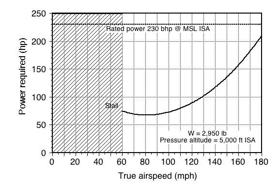
remembering to factor in the propeller efficiency; the power curve is shown in the figure below for a pressure altitude of 5,000 ft where $\varrho_{\infty}$ = 0.002048.

Finally, assuming a constant BSFC gives the fuel flow rate as

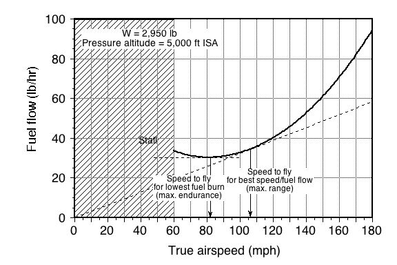
$\frac{dW_f}{dt} = {\overbigdot{W}_f} = c_b P_{\rm req}$

which is shown graphically in the figure below.

The airplane’s endurance and range can be estimated using the appropriate Breguet formulas. This airplane’s fuel capacity is 65 gallons of AVGAS, and at 6.01 lb per gallon, the maximum fuel weight that could be carried would be 390.65 lb. This is about 13% of the gross weight, so the assumption of constant weight over the flight time is reasonable for evaluating the maximum values of $C_L/C_D$ and $C_L^{\, 3/2}/C_D$ . While these values and their corresponding airspeeds will change with weight and altitude, a representative weight that can be used for analysis is that the in-flight weight equals the GTOW less half of the total fuel weight.

Not all of this fuel would be usable, however, because at least some quantity of fuel would be needed for startup, taxi, takeoff, and climb, as well as for the descent and landing plus an allowance of 30 minutes of VFR flight or 45 minutes of IFR flight must be included to comply with FAA regulations. If an average fuel burn allowance of 120 lb is assumed, which seems reasonable for takeoff and landing, this leaves 270 lb of fuel for actual flight use. So, for the endurance and range estimates in this case, then $W_0$ = 2,950-60 = 2,890 lb and $W_1$ = 2,890 – 270 = 2,620 lb.

The estimated maximum endurance can be found using

$E = \frac{ \eta_p}{c} \left(\frac{C_L^{\, 3/2}}{C_D}\right) \sqrt{2 \varrho_{\infty} S} \left( \frac{1}{\sqrt{W_0 - W_f}} - \frac{1}{\sqrt{W_0} } \right)$

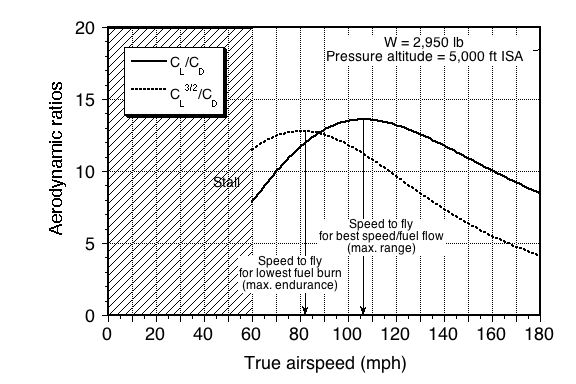
From the graph below, the maximum value of $C_L^{\, 3/2}/C_D$ is 12.79 at 81 mph or 118.8 ft/s.

Notice that the BSFC value must be converted into appropriate engineering units so $c_b$ = 0.45/550/3600 = 2.27 $\times 10^{-7}$ in units of (lb) (lb-ft s $^{-1}$ ) $^{-1}$ (s) $^{-1}$ . Substituting the appropriate values gives

$\begin{eqnarray*} E & = & \frac{0.8 \times 12.79}{2.27 \times 10^{-7}} \sqrt{2 \times 0.002048 \times 174} \left( \frac{1}{\sqrt{2,620}} - \frac{1}{\sqrt{2,890} } \right) \\[10pt] & = & 35,582 \mbox{s} = 593~\mbox{mins} = 9.9 \mbox{hrs} \nonumber \end{eqnarray*}$

So, if we loiter, the airplane at or around an airspeed of 81 mph would stay in the air for nearly 10 hours.

The estimated maximum range can be found using

$R = \frac{\eta_p}{c} \left( \frac{C_L}{C_D}\right) \ln \left( \frac{W_0}{W_0-W_f}\right)$

The maximum value of $C_L/C_D$ is 13.6 at 106 mph or 155 ft/s.
Substituting the appropriate values gives

$\begin{eqnarray*} R & = & \frac{0.8 \times 13.6}{2.27 \times 10^{-7}} \ln \left( \frac{2,890}{2,620} \right) \\[10pt] & = & 3.73\times 10^6 \mbox{ft} = 707 \mbox{miles} \nonumber \end{eqnarray*}$

which would only be obtained if this airplane was flown at or around 106 mph. Of course, this is rather slow compared to the top speed of the airplane, which is around 170 mph, but at that airspeed, the range would be reduced by nearly half.

Remember that these latter results are only estimates of the maximum range and endurance, but they are typically within 10% of the actual values that can be demonstrated in flight.

Worked Example #8

It is desired to estimate the endurance and range of a jet-powered airplane in the form of a small jet similar to the Cessna Citation. The parameters describing this airplane are listed in the table below.

Wing span

$b$

53.3 ft

Wing area

$S$

318 ft $^2$

Wing aspect ratio

$A\!R$

8.93

Gross takeoff weight

$W_{\rm GTOW}$

19,815 lb

Fuel capacity (tankage)

$V_f$

1,119 U.S. gals JET-A

Engine rated thrust ( $\times$ 2)

$T_A$

3,650 lb @ MSL ISA

Engine TSFC

$c_t$

0.6 lb lb $^{-1}$ hr $^{-1}$

Parasitic drag coefficient

$C_{D_{0}}$

0.02

Oswald’s efficiency factor

$e$

0.81

We can assume for the following calculations that the airplane’s weight is the gross takeoff weight, so $L = W =W_{\rm \scriptsize GTOW}$ , although this assumption will tend to overpredict the fuel burn. Alternatively, one can use the $W_{\rm GTOW}$ less half the total fuel weight, which is usually considered the preferred approach. The drag coefficient for the airplane is

$C_D = C_{D_{0}} + \frac{{C_L}^2}{\pi \, AR e}$

assuming no transonic wave drag. For level flight, then, the total thrust required is

$T_{\rm req} = D = \frac{1}{2} \varrho_{\infty} V_{\infty}^2 S\left(C_{D_{0}} + \frac{{C_L}^2}{\pi \, AR e}\right)$

where

$C_L = \frac{W}{\frac{1}{2} \varrho_{\infty} V_{\infty}^2 S}$

Substituting the known values for our exemplar jet airplane gives the thrust required curve shown below for a pressure altitude of 15,000 ft where $\varrho_{\infty}$ = 0.0014963.

Because this is a twin-engine airplane, each engine would produce half of this required thrust. Assuming a constant TSFC gives the total fuel flow rate as

$\frac{dW_f}{dt} = {\overbigdot{W}_f} = c_t T_{\rm req}$

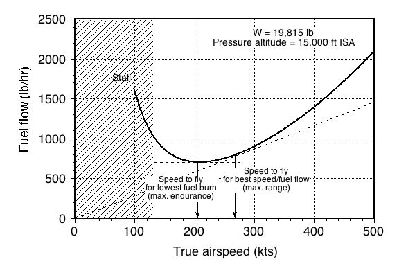
which is shown in the figure below. Notice that the fuel flow mimics the thrust requirements, and for flight at higher airspeeds, the fuel flow increases rapidly, reflecting that for any airplane, there is a high fuel cost involved in flying fast.

Using the appropriate Breguet formulas, we can estimate this jet airplane’s endurance and range. We should always use the proper formulas for jet airplanes and distinguish them from propeller airplanes.

The fuel capacity of this jet airplane is 1,119 gals of JET-A, and at 6.8 lb per gallon, the maximum fuel weight would be 7,609.2 lb, which is about 38% of the airplane’s gross weight. This is why a more accurate estimate of endurance and range would be done using $W_{\rm GTOW}$ less half the total fuel weight. But we will continue here with $W =W_{\rm \scriptsize GTOW}$ . Not all this fuel would be usable, and allowances are needed for previously discussed reasons. We can proceed by assuming that $W_0$ = 19,815 -1,000 (the 1,000 lb being the allowance) = 18,815 lb and $W_1$ = 18,815 – 5,600 = 13,215 lb. The endurance is evaluated by using

$E = \frac{1}{c_t} \left( \frac{C_L}{C_D} \right) \ln \left(\frac{W_0}{W_0 - W_f} \right)$

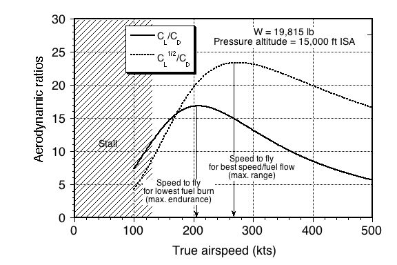
According to the results given below, this airplane’s best $C_L/C_D$ ratio of 16.85 occurs at an airspeed of 208 kts or 351 ft/s. The needed ratios can also be calculated because we have formulas for calculating both $C_L$ and $C_D$ .

Substituting the numbers and remembering to convert $c_t$ into units of s $^{-1}$ by dividing by 3,600 gives

$E = \left(\frac{1}{0.6/3,600} \right) \left( 16.85 \right) \ln \left(\frac{18,815}{13,215} \right) = 9.9 \mbox{~hrs} \nonumber$

where the final result has been converted back from seconds to hours. The range is evaluated by using

$R = \frac{2}{c_t} \sqrt{ \frac{2}{\varrho_{\infty} S}} \left(\frac{C_L^{1/2}}{C_D} \right) \left( W_0^{1/2} - W_1^{1/2} \right)$

The best $C_L^{1/2}/C_D$ ratio of 23.4 occurs at an airspeed of 274 kts or 462 ft/s. Substituting the actual numbers gives

$\begin{eqnarray*} R & = & \frac{2 \times 3,600}{0.6} \sqrt{ \frac{2}{0.0014963 \times 318}} \left( 23.4 \right) \left(18,815^{1/2} - 13,215^{1/2} \right) \nonumber \\[10pt] & = & 2,422 \mbox{~statute~miles} \end{eqnarray*}$

which seems fairly reasonable for this class of jet-powered airplanes. Of course, these results would depend on the payload, which may need to be traded for fuel. Note: For all aircraft, a maximum useful load can be carried, which is the sum of the payload and the fuel load. More payload (e.g., passengers) may and usually does, allow for less fuel load.

Worked Example #9

A small jet airplane weighs 10,000 lb, has a wing area of 200 ft $^2$ , and a drag polar given by $C_D = 0.02 + 0.05 C_L2$ . Because of a fuel leak, the airplane runs out of fuel, and the engines stop at an altitude $h$ = 20,000 ft. Estimate the best glide range from this altitude.

The drag polar is given by

$C_D = 0.02 + 0.05 C_L^ {\,2}$

Therefore,

$\frac{C_D}{C_L} = \frac{0.02}{C_L} + 0.05 C_L$

Differentiating with respect to $C_L$ gives

$\frac{(C_D/C_L)}{C_L} = -\frac{0.02}{C_L^ {\,2}} + 0.05$

which will be zero for a maximum or minimum, i.e.,

$-\frac{0.02}{C_L^ {\,2}} + 0.05 = 0$

or

$C_L = \sqrt{ \frac{0.02}{0.05}} = 0.632$

The drag coefficient at this lift coefficient is

$C_D = 0.02 + 0.05 \times 0.632^2 = 0.04$

Therefore, the lift-to-drag ratio is

$\frac{C_L}{C_D} = \frac{0.632}{0.04} = 15.81$

The gliding distance is given by

$R = h \left( \frac{C_L}{C_D} \right) = 20,000 \times 15.81 = 316,227~\mbox{ft} \approx 52~\mbox{nautical~miles}$

Worked Example #10 – Propellant needed for a single-stage rocket

A single-stage rocket must provide a speed of 6,000 m/s (6 km/s) to a payload mass, $M_L$ , of 12,000 kg. The vehicle’s structural mass coefficient, $\epsilon$ , is 0.06. The propellant used in the engine has a specific impulse, $I_{\rm sp}$ , of 325 s. What must be the rocket’s initial mass, $M_0$ , and its propellant mass, $M_P$ , to meet these requirements?

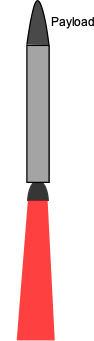
The equivalent exhaust velocity is

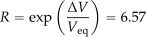
(1) $\begin{equation*} V_{\rm eq} = I_{\rm sp} \, g_0 = 3,188~\mbox{m s$^{-1}$} \end{equation*}$

The initial mass-to-burnout mass ratio, $R$ , is

(2) $\begin{equation*} R = \exp \left( \frac{\Delta V}{V_{\rm eq}} \right) = 6.57 \end{equation*}$

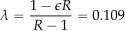
and the payload ratio, $\lambda$ , is

(3) $\begin{equation*} \lambda = \frac{1 - \epsilon R}{R - 1} = 0.109 \end{equation*}$

where $\epsilon = 0.06$ is the structural mass coefficient. Therefore, the initial mass of the rocket, $M_0$ , is

(4) $\begin{equation*} M_0 = \left( \frac{1+\lambda}{\lambda} \right) M_L = 122,000~\mbox{kg} \end{equation*}$

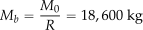
and the burnout mass, $M_b$ , is

(5) $\begin{equation*} M_b = \frac{M_0}{R} = 18,600~\mbox{kg} \end{equation*}$

Finally, the propellant mass, $M_P$ , is

(6) $\begin{equation*} M_P = M_0 - M_b = 122,000 - 18,600 = 103,400~\mbox{kg} \end{equation*}$

which is a fairly large rocket.

Worked Example #11

A small rocket is launched vertically from the Earth’s surface with an initial mass of 1,000 kg. If the rocket engine has a thrust of 10 kN and a specific impulse of 250 s, calculate (a) The rocket’s acceleration at liftoff. (b) The flight velocity of the rocket after 30 seconds.

(a) The acceleration at liftoff will be

$a = \frac{T}{M_0} = \frac{10,000}{1,000} = 10.0~\mbox{m s$^{-2}$}$

(b) The equivalent exhaust velocity is

$V_{\rm eq} = I_{\rm sp} g_0 = 250.0 \times 9.81 = 2,452.5~\mbox{m s$^{-1}$}$

and the thrust from the engine is

$T = \overbigdot{m} \, V_{\rm eq}$

The mass flow rate is

$\overbigdot{m} = \dfrac{T}{V_{\rm eq}} = \dfrac{10,000}{2,452.5} = 4.0775~\mbox{kg s$^{-1}$}$

Therefore, using the rocket equation, then the flight velocity after $t$ seconds will be

$V_{t} = V_{\rm eq} \, \ln\left(\dfrac{M_0}{M_0 - \overbigdot{m} \, t}\right)$

and inserting the numerical values for $t$ = 30 seconds gives

$V_{30} = 2,452.5 \, \ln \left(\dfrac{1,000}{1,000 - 4.0775 \times 30.0}\right) = 320~\mbox{m s$^{-1}$}$

which is just below the speed of sound.

Worked Example #12

Consider a small single-stage rocket with the following design characteristics: propellant mass = 7,200 kg; structural mass = 800 kg; payload mass = 50 kg. The specific impulse for this rocket is 275 s. The rocket blasts off from Earth and climbs vertically. The burning of the fuel occurs steadily, and the burnout time is 60 seconds. The aerodynamic drag can be neglected, but the effects of gravity should be included. (a) What will be the value of the burnout velocity? (b) Find the thrust generated by the rocket. (c) What is the initial acceleration of the rocket? (d) What will the speed and acceleration of the rocket be 30 seconds into the flight?

(a) The equivalent velocity from the rocket engine will be

$V_{\rm eq} = I_{\rm sp} \, g_0 = 275 \times 9.81 = 2,698~\mbox{m s$^{-1}$}$

The burnout mass $M_b$ has no fuel left so this mass will be the sum of the structural mass and payload mass, i.e.,

$M_b = M_S + M_L = 800 + 50 = 850 \mbox{kg}$

The initial mass of the rocket $M_0$ has all the unburned fuel, so

$M_0 = M_S + M_L + M_p = 800 + 50 + 7,200 = 8,050~\mbox{kg}$

With the gravity loss term included, the burnout velocity of the rocket will be

$\Delta V = V_{\rm eq} \ln \left( \frac{M_0}{M_b} \right) - g_0 \, t_b = 2,698 \times \ln(8050/850) - 9.81 \times 60 = 5,477~\mbox{m s$^{-1}$}$

(b) The thrust generated by the rocket will be

$T = \overbigdot{m}_P \, V_{\rm eq} = \frac{M_P}{t_b} V_{\rm eq} = 7,200/60 \times 2,698 = 323.76~\mbox{kN}$

(c) With the consideration of gravity, the initial acceleration will be

$a = \frac{T - M_0 \, g_0}{M_0} = \frac{323,760 - 8,050 \times 9.81}{8,050} = 30.41~\mbox{m s$^{-2}$ }$

so about 3 $g_0$ .

(d) After 30 secs from liftoff, the mass of the rocket will be

$M_{30} = M_0 - \overbigdot{m}_P \, t = 8,050 - 7,200 \times 30 /60 = 4,450~\mbox{kg}$

and so the acceleration at 30 secs will be

$a_{30} = \frac{T - M_{30} \, g_0}{M_{30}} = \frac{ 323,760 - 4,450 \times 9.81}{4,450} = 62.94~\mbox{m s${^-2}$}$

so about 6 $g_0$ .

$\Delta V_{30} = V_{\rm eq} \ln \left( \frac{M_0}{M_{30}} \right) - g_0 \, t_b = 2,698 \times \ln(8050/4450) - 9.81 \times 30 = 1,305~\mbox{m s$^{-1}$}$

Of course, including aerodynamic drag on the rocket would reduce this value slightly.

Worked Example #13

A single-stage rocket has a total mass of $1.14 \times 10^5$ kg and a burnout mass of $1.11 \times 10^4$ kg, including engines, structural shell, and payload. The rocket blasts off from Earth and climbs vertically, exhausting its propellant in 2.2 minutes. The propellant burning occurs at a steady rate, and the specific impulse of the propulsion system is 240 seconds. (a) If air resistance and gravity are neglected, what will the rocket’s velocity be at burnout conditions? (b) What thrust does the rocket engine develop at liftoff? (c) What is the initial acceleration of the rocket if gravity is not neglected? (d) What is the acceleration of the rocket at 60 seconds into the flight?

(a) We have that specific impulse $I_{\rm sp}$ is 240 seconds and the initial mass $M_0$ is 1.14 $\times 10^5$ kg and the burnout mass $M_b$ is 1.11 $\times 10^4$ kg. Therefore, the propellant mass $M_P$ will be

$M_P = M_0 - M_b = 1.14 \times 10^5 - 1.11 \times 10^4 = 1.029 \times 10^5~\mbox{kg}$

The rocket equation (we are told to ignore the gravity loss term in this equation) gives us the change in the velocity of the vehicle $\Delta V$ , i.e.,

$\Delta V = V_{\rm eq} \ln \left( \frac{M_0}{M_b} \right)$

The equivalent exhaust velocity $V_{\rm eq}$ is given in terms of the specific impulse, i.e.,

$V_{\rm eq} = I_{\rm sp} g_0 = 240.0 \times 9.81 = 2,354.4~\mbox{m s$^{-1}$}$

The burnout velocity is

$\Delta V = V_{\rm eq} \ln \left( \frac{M_0}{M_b} \right) = 2,354.4 \ln \left( \frac{114,000}{11,100} \right) = 5,484~\mbox{m s$^{-1}$} = 5.48~\mbox{km/s}$

if we do not include the gravity loss term, as stated.

(b) We need to find the net mass flow rate to the engines. Assuming the rate of propellant consumption is constant, then the mass of the rocket $M$ varies over time as

$M = M_0 - M_P \left( \frac{t}{t_b} \right) = M_0 - \left( \frac{M_P}{t_b} \right) t = M_0 - \overbigdot{m}_P \, t$

where $t_b$ is the burnout time and $\overbigdot{m}_P$ is the rate of burning propellant. The thrust produced $T$ will be

$T = \overbigdot{m}_P V_{\rm eq} = \left( \frac{M_P}{t_b} \right) V_{\rm eq} = \left( \frac{1.029 \times 10^5}{2.2 \times 60} \right) 2,354.4 = 1.835~\mbox{MN}$

(c) The initial acceleration will be

$a = \frac{T - M_0 g_0}{M_0} = \frac{1.835 \times 10^6 - 1.14 \times 10^5 \times 9.81}{1.14 \times 10^5} = 6.29~\mbox{m s$^{-2}$}$

(d) The mass of the rocket at 60 seconds into the flight will be

$M_{60} = M_0 - \left( \frac{M_P}{t_b}\right) t = 1.14 \times 10^5 - \left( \frac{1.029 \times 10^5}{2.2 \times 60} \right) 60.0 = 67,227.3~\mbox{kg}$

So, the acceleration will be

$a = \frac{T - M_{60} g_0}{M_{60}} = \frac{1.835\times 10^6 - (67,227.3) (9.81)}{67,227.3} = 17.49~\mbox{m s$^{-2}$}$

Worked Example #14

Use the rocket equation to determine its burnout velocity and maximum achievable height, assuming it was launched vertically. Neglect the aerodynamic drag forces. Solve for the burnout velocity and maximum altitude if the burnout time is 60 seconds. The specific impulse is 250 seconds, the initial mass is 12,700 kg, and the propellant mass is 8,610 kg.

We are given that specific impulse $I_{\rm sp}$ is 250 seconds, the initial mass $M_0$ is 12,700 kg, and the propellant mass $M_P$ is 8,610 kg. The rocket equation gives us the change in the velocity of the vehicle $\Delta V$ , i.e.,

$\Delta V = V_{\rm eq} \ln \left( \frac{M_0}{M_b} \right)$

where $M_0$ is the initial mass of the vehicle and $M_b$ is the final or burnout mass. If gravity is included (but no aerodynamic drag), then

$\Delta V = V_{\rm eq} \ln \left( \frac{M_0}{M_b} \right) - g_0 \, t_b.$

where $t_b$ is the burnout time, which is 60 seconds in this case.

The equivalent exhaust velocity $V_{\rm eq}$ is given in terms of the specific impulse, i.e.,

$V_{\rm eq} = I_{\rm sp} g_0 = 250 \times 9.81 = 2,452.5~\mbox{m s$^{-1}$}$

The burnout mass $M_b$ is given by

$M_b = M_0 - M_P = 12,700 - 8,610 = 4,090~\mbox{kg}$

So now we have the burnout velocity, which is

$\Delta V = V_{\rm eq} \ln \left( \frac{M_0}{M_b} \right) = 2,452.5 \ln \left( \frac{12,700}{4,090} \right)$

so

$\Delta V = 2,452 \times 1.133 = 2,778.16~\mbox{m s$^{-1}$} = 2.77~\mbox{km s$^{-1}$}$

if we do not include the gravity loss term. With the gravity loss term included, then

$\Delta V = V_{\rm eq} \ln \left( \frac{M_0}{M_b} \right) - g_0 \, t_b$

So $\Delta V$ at the burnout is reduced to

$\Delta V = 2,778.16 - 9.81 \times 60 = 2,778.16 - 588.6 = 2,189.56~\mbox{m s$^{-1}$} = 2.18~\mbox{km s$^{-1}$}$

Assuming the propellant consumption rate is constant, then the mass of the rocket $M$ varies over time as

$M = M_0 - M_P \frac{t}{t_b} = M_0 - \left( M_0 - M_b \right) \frac{t}{t_b}$

The velocity then is

$V = V_{\rm eq} \ln \left( \frac{M_0}{M} \right) - g_0 t$

The height achieved at the burnout time is then.

$H_b = \int_0^{t_b} V dt$

which, after the application of mathematics, gives

$H_b = V_{\rm eq} t_b \left( \frac{ \ln \left( \displaystyle{\frac{M_0}{M_b}} \right) }{\displaystyle{\frac{M_0}{M_b} - 1} } \right) - \frac{1}{2} g_0 t_b^2$

Inserting the values gives

$H_b = 2,452.5 \times 60 \left( \frac{ \ln \left( \displaystyle{\frac{12,700}{4,090}} \right) }{\displaystyle{\frac{12,700}{4,090} - 1} } \right) - \frac{1}{2} \times 9.81 \times 60^2$

so

$H_b = 2,452.5 \times 60 \left( \frac{1.133}{2.105} \right) - \frac{1}{2} \times 9.81 \times 60^2 = 61,544.5~\mbox{m} = 61.54~\mbox{km}$

The final additional coasting height of the rocket can then be determined by equating the kinetic energy of the rocket at its burnout time with its change in potential energy between that point and the maximum obtained height.

Worked Example #15

A rocket must provide a speed of 6,000 m/s to a payload of 12,000 kg. The vehicle’s structural coefficient is 0.06. The propellants used in the engines have a specific impulse of 325 s. What must the initial mass and propellant mass be to meet these requirements?

The equivalent exhaust velocity

$V_{\rm eq} = I_{\rm sp} g_0 = 3,188.25~\mbox{m s$^{-1}$}$

so

$R = \exp \left( \frac{\Delta V}{V_{\rm eq}} \right) = 6.57$

and

$\lambda = \frac{1 - \epsilon R}{R - 1} = 0.109$

Therefore, the initial mass is

$M_0 = \frac{1+\lambda}{\lambda} M_L = 122,211~\mbox{kg}$

and the burnout mass is

$M_b = \frac{M_0}{R} = 18,613~\mbox{kg}$

so the propellant mass is

$M_p = M_0 - M_b = 103,598~\mbox{kg}$

Worked Example #16

Use the rocket equation to determine a rocket’s burnout velocity and maximum achievable height if its burnout time is 60 seconds. The specific impulse is 250 seconds, the initial mass is 12,700 kg, and the propellant mass is 8,610 kg. Assume the rocket is launched vertically.

The specific impulse $I_{\rm sp}$ is 250~seconds, the initial mass $M_0$ is 12,700 kg, and the propellant mass $M_p$ is 8,610 kg. The rocket equation gives us the change in the velocity of the vehicle $\Delta V$ , i.e.,

$\Delta V = V_{\rm eq} \ln \left( \frac{M_0}{M_b} \right)$

where $M_0$ is the initial mass of the vehicle and $M_b$ is the final or burnout mass. If gravity is included (but no aerodynamic drag), then

$\Delta V = V_{\rm eq} \ln \left( \frac{M_0}{M_b} \right) - g_0 \, t_b.$

where $t_0$ is the burnout time, which is 60 seconds in this case.

The equivalent exhaust velocity $V_{\rm eq}$ is given in terms of the specific impulse, i.e.,

$V_{\rm eq} = I_{\rm sp} g_0 = 250 \times 9.81 = 2,452.5~\mbox{m s$^{-1}$}$

The burnout mass $M_b$ is given by

$M_b = M_0 - M_P = 12,700 - 8,610 = 4,090~\mbox{kg}$

So now we have the burnout velocity, which is

$\Delta V = V_{\rm eq} \ln \left( \frac{M_0}{M_b} \right) = 2,452.5 \ln \left( \frac{12,700}{4,090} \right)$

so

$\Delta V = 2,452 \times 1.133 = 2,778.16~\mbox{m s$^{-1}$} = 2.77~\mbox{km s$^{-1}$}$

if we do not include the gravity loss term. With the gravity loss term included, then

$\Delta V = V_{\rm eq} \ln \left( \frac{M_0}{M_b} \right) - g_0 \, t_b$

So $\Delta V$ at the burnout is reduced to

$\Delta V = 2,778.16 - 9.81 \times 60 = 2,778.16 - 588.6 = 2,189.56~\mbox{m s$^{-1}$} = 2.18~\mbox{km s$^{-1}$}$

Assuming the propellant consumption rate is constant, then the mass of the rocket $M$ varies over time as

$M = M_0 - M_P \frac{t}{t_b} = M_0 - \left( M_0 - M_b \right) \frac{t}{t_b}$

The velocity is

$V = V_{\rm eq} \ln \left( \frac{M_0}{M} \right) - g_0 t$

The height achieved at the burnout time is then.

$H_b = \int_0^{t_b} V dt$

which, after some mathematics, gives

$H_b = V_{\rm eq} t_b \left( \frac{ \ln \left( \displaystyle{\frac{M_0}{M_b}} \right) }{\displaystyle{\frac{M_0}{M_b} - 1} } \right) - \frac{1}{2} g_0 t_b^2$

Inserting the values gives

$H_b = 2,452.5 \times 60 \left( \frac{ \ln \left( \displaystyle{\frac{12,700}{4,090}} \right) }{\displaystyle{\frac{12,700}{4,090} - 1} } \right) - \frac{1}{2} \times 9.81 \times 60^2$

so

$H_b = 2,452.5 \times 60 \left( \frac{1.133}{2.105} \right) - \frac{1}{2} \times 9.81 \times 60^2 = 61,544.5~\mbox{m} = 61.54~\mbox{km}$

The final additional coasting height of the rocket can then be determined by equating the kinetic energy of the rocket at its burnout time with its change in potential energy between that point and the maximum obtained height.

Worked Example #17

Consider a two-stage rocket with a payload mass = 60 kg. The first stage has two solid rocket boosters attached. First stage: propellant mass = 7,200 kg, structural mass = 800 kg, and mass flow rate = 80.0 kg s $^{-1}$ . For each booster, propellant mass = 1,400 kg, structural mass = 200 kg, and the burn time is 45 s. For the second stage: propellant mass = 5,400 kg, structural mass = 600 kg. The specific impulse for the first stage is 250 and 290s for the boosters. Find the extra burnout velocity of the rocket at first stage separation when using the boosters compared to without the boosters.

Here is a summary of the information provided:

Propellant mass for stage 1, $M_{P_{1}}$ = 7,200 kg
Propellant mass for stage 2, $M_{P_{2}}$ = 5,400 kg
Propellant mass for each booster, $M_{P_{b}}$ = 1,400 kg
Structural mass for stage 1, $M_{S_{1}}$ = 800 kg
Structural mass for stage 2, $M_{S_{2}}$ = 600 kg
Structural mass for each booster, $M_{S_{b}}$ = 200 kg
Payload mass, $M_{L}$ = 60 kg
Specific impulse for stage 1, $I_{{\rm SP}_{1}}$ = 250.0 s
Specific impulse for boosters, $I_{{\rm SP}_{b}}$ = 290.0 s
Burnout time for each booster, $t_{b_{b}}$ = 45 s
Mass flow rate for stage 1, $\overbigdot{m}_1$ = 80 kg/s

The initial mass, $M_0$ , of the rocket without the boosters is

$M_0 = M_{P_{1}} + M_{P_{2}} + M_{S_{1}} + M_{S_{2}} + M_{L}$

and inserting the values gives

$M_0 = 7,200.0 + 5,400.0 + 800.0 + 600.0 + 60.0 = 14,060.0~\mbox{kg}$

The burnout mass, $M_b$ , just before the first stage separation is

$M_b = M_{P_{2}} + M_{S_{1}} + M_{S_{2}} + M_{L}$

which gives the burnout mass, $M_b$ , as

$M_b = 5,400.0 + 800.0 + 600.0 + 60.0 = 6,860.0~\mbox{kg}$

Therefore, the $\Delta V$ increment for the first stage without the boosters is

$\Delta V = V_{b_{1}} = V_{{{\rm eq}_{1}}} \ln \left( \frac{M_0}{M_b} \right) - g_0 \, t_b$

and inserting the values gives

$V_{b_{1}} = 2,452.5 \, \ln \left( \frac{14,060.0}{6,860.0} \right) - 9.81\times 90 = 877.08~\mbox{m s$^{-1}$}$

Therefore, for the first stage, the burnout velocity is

$V_{b_{1}} = 877.08~\mbox{m s$^{-1}$}$

The equivalent exhaust velocity for each booster, $V_{{\rm eq}_{b}}$ , is

$V_{{\rm eq}_{b}} = I_{{\rm SP}_{b}} \, g_0 = 290 \times 9.81 = 2,844.9~\mbox{m s$^{-1}$}$

and the net thrust, $T_b$ , produced is

$T_b = 2 \overbigdot{m}_b\, V_{{\rm eq}_{b}}$

The mass flow rate for each booster is

$\overbigdot{m}_b = \frac{M_{P_{1}}}{t_{b_{1}}} = \frac{1,400}{45} = 31.1~\mbox{kg s$^{-1}$}$

so the net thrust (to augment the thrust of stage 1) will be

$T_b = 2 \times 31.1 \times 2,844.9 = 177,016 ~\mbox{N} = 177.016~\mbox{kN}$

remembering that there are two boosters. Notice that the boosters nearly double the thrust at the launch.

To obtain the burnout velocity at booster burnout at 45 seconds into the flight, we first need the mean equivalent exhaust velocity for the stage 1 core and the two boosters, which is given by

$\overline{V}_{\rm eq} = \frac{ N_b \, \overbigdot{m}_b \, V_{{\rm eq}_{b}} + \overbigdot{m}_1 \, V_{{{\rm eq}_{1}}} }{ N_b \overbigdot{m}_b + \overbigdot{m}_1 }$

where $N_b = 2$ . The mass flow rates and the equivalent velocities of the stage 1 core and the boosters have already been calculated, so

$\overline{V}_{\rm eq} = \frac{ 2 \times 31.1 \times 2,844.9 + 80.0 \times 2,452.5}{ 2 \times 31.1 + 80.0} = 2,624.14~\mbox{m s$^{-1}$}$

The burnout velocity of the rocket at booster burnout, $V_{b_{b}}$ , at $t_{b_{b}}$ = 45 seconds into the flight is given by

$V_{b_{b} } = \overline{V}_{\rm eq} \ln \left( \frac{M_0}{M_b} \right) - g_0 \, t_{b_{b}}$

In this case, the initial mass, $M_0$ , of the rocket with the two boosters is

$M_0 = M_{P_{1}} + M_{P_{2}} + M_{S_{1}} + M_{S_{2}} + M_{L} + 2 M_{S_{b}} + 2 M_{P_{b}}$

and inserting the values gives

$M_0 = 7,200.0 + 5,400.0 + 800.0 + 600.0 + 60.0 + 2 \times 1,400.0 + 2 \times 200.0 = 17,260.0~\mbox{kg}$

The burnout mass, $M_b$ , at booster burnout at 45 seconds is

$M_b = \left( \frac{90.0 - 45.0}{90} \right) M_{P_{1}} + M_{P_{2}} + M_{S_{1}} + M_{S_{2}} + M_{L} + 2 M_{S_{b}}$

noting that the first stage core has burned, in this case, half of its propellant. Therefore, the burnout mass at booster burnout, $M_b$ , is

$M_b = 0.5 \times 7,200.0 + 5,400.0 + 800.0 + 600.0 + 60.0 + 2 \times 200.0 = 10,860~\mbox{kg}$

Therefore, the $\Delta V$ increment for the first stage at the burnout time is

$\Delta V_b = \overline{V}_{\rm eq} \ln \left( \frac{M_0}{M_b} \right) - g_0 \, t_{b_{b}}$

and inserting the values gives

$\Delta V_b = 2,624.14 \, \ln \left( \frac{17,260.0}{10,860.0} \right) - 9.81\times 45 = 774.33~\mbox{m s$^{-1}$}$

Therefore, at booster burnout, the velocity of the rocket is

$V_{b_{b}} = 774.33~\mbox{m s$^{-1}$}$

The first stage then burns for another 45 seconds, over which it burns the other half of its propellant. After booster separation, the new initial weight is

$M_0 = 0.5 \times 7,200.0 + 5,400.0 + 800.0 + 600.0 + 60.0 = 10,460.0~\mbox{kg}$

and the burnout mass just before stage 1 separation is then

$M_b = M_{P_{2}} + M_{S_{1}} + M_{S_{2}} + M_{L}$

Therefore, the burnout mass is

$M_b = 5,400.0 + 800.0 + 600.0 + 60.0 = 6,860~\mbox{kg}$

and so the $\Delta V$ for this part of the launch is

$\Delta V_1 = V_{{{\rm eq}_{1}}} \ \ln \left( \frac{M_0}{M_b} \right) - g_0 \, t_{b_{b}}$

Inserting the values gives

$\Delta V_1 = 2,452.5 \, \ln \left( \frac{10,460}{6,860} \right) - 9.81\times 45 = 593.14~\mbox{m s$^{-1}$}$

Therefore, at stage 1 burnout, the velocity of the rocket is

$V_{b_{1}} = 774.33 + 593.14 = 1,367.5~\mbox{m s$^{-1}$}$

This means the rocket travels nearly twice the velocity it would have traveled without the boosters.

Worked Example #18 – Space Shuttle launch

Consider a Space Shuttle launch, which is a parallel rocket system launch vehicle. The Shuttle used LH₂/LOX for the “core” main engines on the Orbiter, with two solid rocket boosters or SRBs. It is required to estimate the final burnout velocity. Neglect the gravity loss term in the rocket equation. The information available includes the following:

Orbiter:
- Structural mass = 110,000 kg
- Payload mass = 24,000 kg
- Specific impulse = 454 seconds
- Burnout time = 480 seconds

External tank
- Structural mass = 30,000 kg
- Propellant mass = 720,000 kg

SRB (for each):
- Structural mass = 86,000 kg
- Propellant mass = 500,000 kg
- Specific impulse = 269 seconds
- Burnout time = 124 seconds

For the Orbiter or the “core,” the equivalent exhaust velocity, $V_{{\rm eq}_{c}}$ , is

$V_{{\rm eq}_{c}} = I_{\rm sp_{c}} \, g_0 = 454 \times 9.81 = 4,453.7~\mbox{m s$^{-1}$}$

For the SRBs, the equivalent exhaust velocity, $V_{{\rm eq}_{b}}$ , is

$V_{{\rm eq}_{b}} = I_{\rm sp_{b}} \, g_0 = 269 \times 9.81 = 2,638.9~\mbox{m s$^{-1}$}$

The fraction of propellant mass remaining in the core at booster burnout will be

$\chi = \frac{480 - 124}{480} = 0.742$

The mean equivalent exhaust velocity, $\overline{V}_{\rm eq}$ , is

$\overline{V}_{\rm eq} = \frac{ M_{P_{b}} \, V_{{\rm eq}_{b}} + (1 - \chi) \, M_{P_{c}} \, V_{{{\rm eq}_{c}}} }{ M_{P_{b}} + (1 - \chi) M_{P_{c}}}$

and putting in the values gives

$\begin{eqnarray*} \overline{V}_{\rm eq} & = & \frac{ 2 \times 500,000 \times 2,638.9 + (1 - 0.742) \times 720,000 \times 4,453.7}{2 \times 500,000 + (1 - 0.742)\times 720,000} \\ & & = 2,923.2~\mbox{m s$^{-1}$} \end{eqnarray*}$

The initial mass at the point of launch is

$M_{0_{0}} = M_{P_{c}} + M_{P_{b}} + M_{S_{c}} + M_{S_{b}} + M_{L}$

and putting in the values gives

$\begin{eqnarray*} M_{0_{0}} & = & (720,000 + 2 \times 500,000) + (110,000 + 30,000) + \\ & & \quad \quad \quad \quad \quad \quad (2 \times 86,000) + 24,000 \\ & = & 2,056,000~\mbox{kg} \end{eqnarray*}$

The final mass of the vehicle at SRB burnout is

$M_{f_{0}} = \chi M_{P_{c}} + M_{S_{c}} + M_{S_{b}} + M_{L}$

and putting in the values gives

$M_{f_{0}} = 0.742 \times 720,000 + (110,000 + 30,000) + 2 \times 86,000 + 24,000 = 870,240~\mbox{kg}$

Therefore, the $\Delta V$ at SRB burnout is

$\Delta V_0 = \overline{V}_{\rm eq} \ln \left( \frac{M_{0_{0}}}{M_{f_{0}} } \right) = 2,923.2 \ln \left( \frac{2,056,000}{870,240} \right) = 2,512.2~\mbox{m s$^{-1}$}$

The initial vehicle mass after SRB separation is

$M_{0_{1}} = \chi M_{P_{c}} + M_{S_{c}} + M_{L}$

and putting in the values gives

$M_{0_{1}} = 0.742 \times 720,000 + (110,000 + 30,000) + 24,000 = 698,240~\mbox{kg}$

The final mass at the depletion of the propellant in the external tank is

$M_{f_{1}} = M_{S_{c}} + M_{L} = (110,000 + 30,000) + 24,000 = 164,000~\mbox{kg}$

The extra $\Delta V$ at complete burnout is

$\Delta V_1 = V_{{\rm eq}_{c}} \ln \left( \frac{M_{0_{1}}}{M_{f_{1}}} \right) = 4,453.7 \ln \left( \frac{698,240}{164,000} \right) = 6,453.1~\mbox{m s$^{-1}$}$

Therefore, the final burnout velocity of the Orbiter is

$V_f = \Delta V_0 + \Delta V_1 = 2,512.2 + 6,453.1 = 8,965.3~\mbox{m s$^{-1}$} \approx 9~\mbox{km s$^{-1}$}$

which is fairly close to the values quoted by NASA, bearing in mind that the gravitational $\Delta V$ has been neglected.

Worked Example #19 – Change in kinetic energy of a spacecraft

A spacecraft with a mass of 10,000 kg travels with a velocity of 5,000 m/s. If its rocket engine with a specific impulse of 250 seconds is turned on and produces a constant thrust of 50 kN for 100 seconds, then calculate (a) The final velocity of the spacecraft. (b) The change in kinetic energy of the spacecraft.

(a) The final velocity of the spacecraft is given by

$V_f = V_i + a \; t = V_i +\left( \dfrac{T}{M} \right) t = 5,000.0 + \left( \frac{50,000}{10,000} \right) 100.0 = 5,500~\mbox{m s$^{-1}$}$

(b) The change in kinetic energy of the spacecraft is given by

$\Delta KE = \frac{1}{2} M_f V_f^2 - \frac{1}{2} M_i V_i^2$

The initial mass of the spacecraft is 10,000 kg, and the final mass can be determined based on the mass flow rate, i.e.,

$\overbigdot{m} = \frac{T}{I_{\rm sp} \, g_0} = \frac{20,000}{250.0 \times 9.81} = 8.155~\mbox{kg s$^{-1}$}$

giving the final mass as

$M_f = M_i - \overbigdot{m} \, t_b = 10,000 - 8.155 \times 100.0 = 9,184.5~\mbox{kg}$

Therefore, the change in kinetic energy of the spacecraft is

$\Delta KE = \frac{1}{2} \times 9,184.5 \times 5,500^2 - \frac{1}{2} \times 10,000 \times 5,000^2 = 1.39 \times 10^4~\mbox{MJ}$

License

Icon for the Creative Commons Attribution-NonCommercial-NoDerivatives 4.0 International License

Introduction to Aerospace Flight Vehicles Copyright © 2022–2024 by J. Gordon Leishman is licensed under a Creative Commons Attribution-NonCommercial-NoDerivatives 4.0 International License, except where otherwise noted.