15 Dimensional Analysis
Introduction
Engineers quickly begin to recognize from even the most casual observations that understanding and solving real-world problems involves considering many parameters, as well as parameters with other dependencies and interdependencies. In other words, many quantities and factors could affect the physical behavior of a given system, and different effects will be obtained when one parameter is varied versus another. In particular, the behavior of air and other fluids is relatively complex to describe because they can be sheared and deformed, primarily as they flow around objects; notice that objects are often referred to as “bodies” in the field of fluid dynamics.
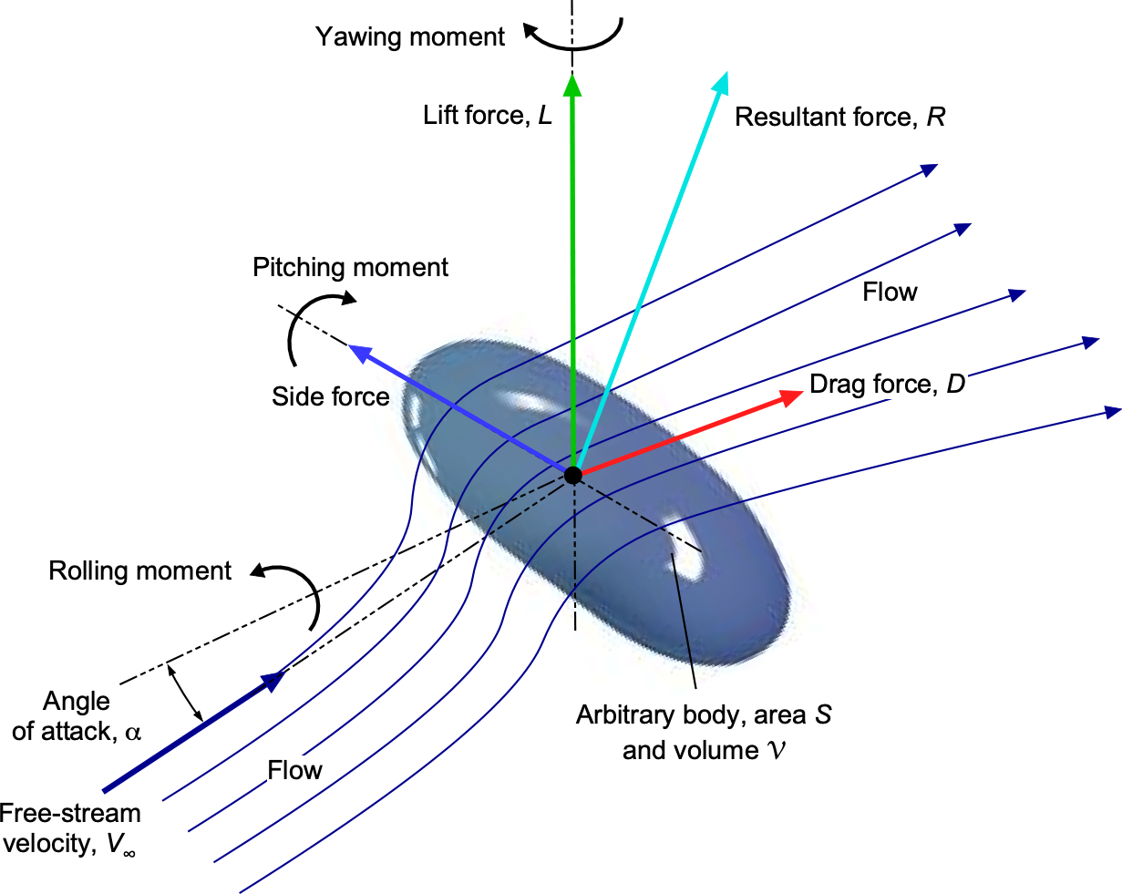
The fluid also produces forces and moments on such bodies, including the familiar lift and drag forces, as shown in the figure below. There is undoubtedly an intuitive expectation that what the flow does (e.g., where the fluid goes) and what effects it has on the body will be determined at least partially by the geometrical shape of the body, as well as its angular orientation to the flow. The forces can also be expected to depend on the fluid properties already discussed, such as flow velocity (airspeed), density, viscosity, temperature, pressure, and speed of sound, among others. However, other parameters may also be involved.
To solve this type of fluid dynamics problem, one approach would be to derive and use the equations of motion governing the fluid’s behavior, and then attempt to solve these equations. These nonlinear partial differential equations, known as the Navier-Stokes equations, form the basis of a class of methods called computational fluid dynamics (CFD). However, this is not a straightforward approach due to the complexity of the nonlinear partial differential equations that must be solved, as well as the considerable proficiency required in the solution methods.
Another approach would be to conduct experiments to determine the relationships between the forces acting on a body and the fluid properties, for example, in tests performed in a wind tunnel. At least in principle, either or both of these latter approaches will enable the determination of the effects of the fluid on the body, as well as the reciprocal influences of the body on the fluid. However, even with CFD and the ability to conduct experiments, sequential variations in the problem parameters to determine cause and effect will take a considerable amount of time.
Nevertheless, another method can be used to help determine the general effects of key physical quantities on aerodynamic behavior. This method is called dimensional analysis, which reduces the number of unknowns governing the understanding of the problem into sets of dimensionless or non-dimensional groupings called similarity parameters. These similarity parameters then allow a significant simplification in understanding the effects of the original problem parameters. Another advantage of dimensional analysis is its ability to help predict the behavior of a given system at a larger scale from results known at a smaller scale, a principle crucial in many aspects of engineering design. Dimensional analysis is not restricted to fluid problems and is helpful in many fields of engineering and science.
Learning Objectives
- Appreciate the principle of dimensional homogeneity and balancing the dimensions of an equation.
- Understand how to perform dimensional analysis, a method used to identify the primary dependencies in an engineering problem in terms of dimensionless groupings, called similarity parameters.
- Realize the significance of dimensionless similarity parameters and how they can simplify a problem and reduce the number of dependencies, i.e., making a problem more straightforward to comprehend.
- Develop and discuss some exemplary problems to become familiar with the method and practice of dimensional analysis and the use of similarity parameters.
Physical Quantities
Recall that physical quantities are of two types: base quantities and derived quantities. Base quantities, such as mass, length, time, and temperature, can be readily measured and observed. Derived quantities are things like velocity, pressure, energy, and power, all of which are derived from these base quantities. In dimensional analysis, only base quantities are used; those encountered in mechanics and engineering are listed in the table below. Other base quantities that may arise in problem-solving are electrical current (Ampere or Amp), the intensity of light (candela), and concentration (mole). Notice also that unit symbols are generally not italicized. For example, the symbol for length is  , but the symbol for the base dimension of length is L. Likewise, the symbol for temperature is
  , but the symbol for the dimension of temperature is
  .
.
| Base quantity | Symbol | Base dimension | SI unit | USC unit |
| Mass | M | M | kilogram (kg) | slug (or slugs or sl) |
| Length | L | L | meter (m) | foot (ft) |
| Time | t | T | second (s) | second (s) |
| Temperature | T | |
Kelvin ( K or K) K or K) |
Rankine (R or R) |
Many of the parameters routinely used in engineering are derived parameters, in that their units are derived from combinations of base dimensions, e.g., volume, density, force, work, energy, power, etc. Consider the following examples of derived parameters, noting that a parameter inside a set of square brackets [ ] means the dimensions of that parameter, i.e.,
(1) ![\begin{equation*} \left[ \text{parameter} \right] \equiv \text{dimensions of that parameter} \end{equation*}](https://eaglepubs.erau.edu/app/uploads/quicklatex/quicklatex.com-20d9f60cc572a2d5e099c5cde21e16bc_l3.svg "Rendered by QuickLaTeX.com")
- Velocity,
 , is distance per unit time, i.e., L/T = L T
 . Notice also that scientific notation must be used throughout dimensional analysis to avoid ambiguity in the final dimensions of the derived parameter. Therefore, [] = L T.
 - Volume,
 , is the volume of something such as a cuboid, then its width (dimensions of L) must be multiplied by its length (dimensions of L) by its height (dimensions of L). Therefore, the derived units for volume are L
 or [] = L.
 - The density,
 , of some substance, is its mass (dimensions of M) per unit volume (dimensions of L), so density will have dimensions of M L
 , i.e., [] = M L.
 - A force is equivalent to the product of a mass and its acceleration (Newton’s second law), so in terms of its base dimensions, then [
 ] = M LT
 .
. - Torque, given the symbol
 or , is a moment, so the product of a force times a distance or “arm.” Therefore, []
  [] = (M LT) L = M L
 T.
T.
Obtaining the correct base dimensions of any given parameter takes some practice, but it is essential for correctly using dimensional analysis. Again, the scientific notation should be used when expressing the dimensions of a parameter to avoid ambiguity, e.g., always use the form M L T and not M L / T .
.
Aerodynamic Force on a Wing
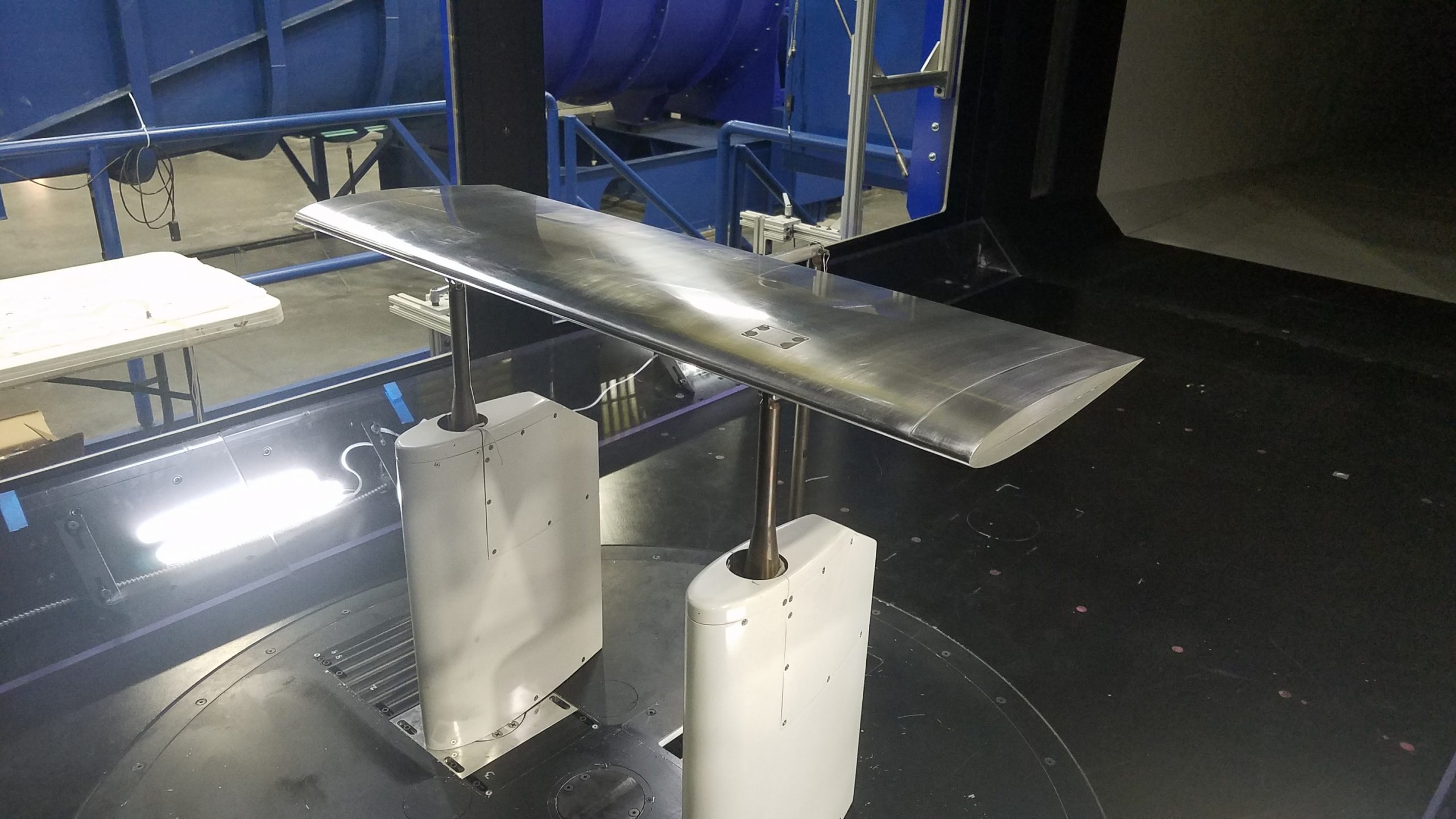
To introduce dimensional analysis methods, consider the forces produced on a wing placed in the test section of a wind tunnel, as shown in the photo below. The resultant aerodynamic force on the wing is  . For convenience, it can be assumed that this force acts at a center of pressure, which, by definition, is a point where there are no pitching moments. In 1687, Philosophiae Naturalis Principia Mathematica (Mathematical Principles of Natural Philosophy) made three statements say that the forces acting on two geometrically similar bodies which move in fluids with different densities are proportional to:
- The square of the velocity of the fluid.
- The square of the linear dimension of the body.
- The density of the fluid.
He further notes that the proportionality of the force to the square of the velocity is restricted to lower flow speeds because ballistic experiments, even in Newton’s time, suggested that these statements do not apply to flow velocities greater than the speed of sound. Under these conditions, the thermodynamics of the fluid flow will also become important.
In general, for a subsonic flow, it would be expected that the resultant aerodynamic force on the wing for a given orientation to the flow will depend on:
- The freestream velocity,
 .
. - The freestream density,
 .
. - The size of the wing, as described by its planform area
 , which for a rectangular wing is the product of its chord
  and span
  , i.e.,
  , as shown in the figure below.
 - The sonic velocity
 , i.e., the potential for compressibility effects.
 - The viscosity of the air, i.e., on the coefficient of viscosity
 .
.
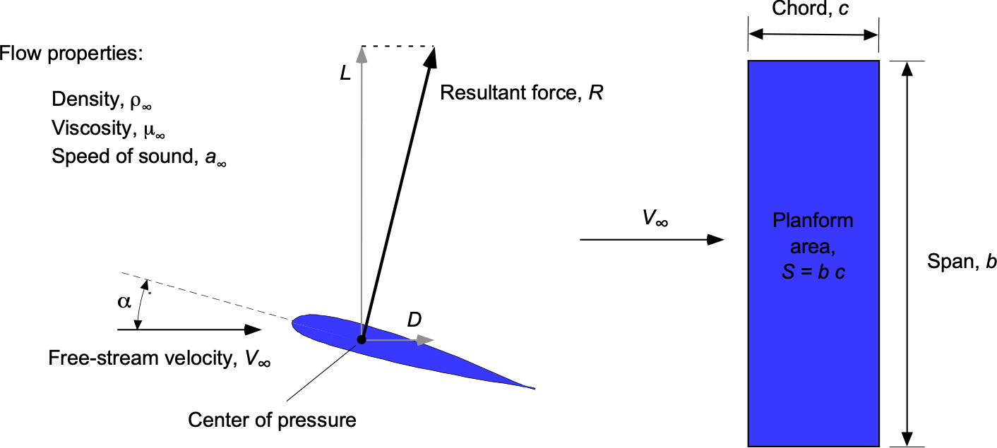
The subscript  or “infinity” means undisturbed conditions, i.e., the “freestream” or reference values of these quantities that are constant well upstream of the wing. Defining fixed reference values is logical because otherwise, all of these values will change as the flow approaches the wing. Notice that the angle of attack of the wing,
  , is the angle between the chordline of the wing (i.e., a line running from the leading edge or nose to the trailing edge or tail of the wing) and the direction of the freestream velocity .
The relationship between and the air properties may now be written in a general functional form as
(2) 
where is referred to as the dependent variable and , , and are called the independent variables. The functional dependence, i.e., the relationship(s) between the dependent and independent variables, denoted by  in this case, is still to be determined, which, more often than not, is determined from experiments.
Although this equation expresses a general relationship, its direct use for measuring or calculating is often impractical. To understand why, consider how an engineering student might measure in a wind tunnel experiment. The student could begin by placing a wing at a given angle of attack, , and then systematically varying each of the influencing parameters, , , , and , one at a time, measuring the corresponding values of at each step. This process is known as a parametric study. The student might return with a series of plots illustrating the dependencies of on each parameter, such as shown in the figure below.
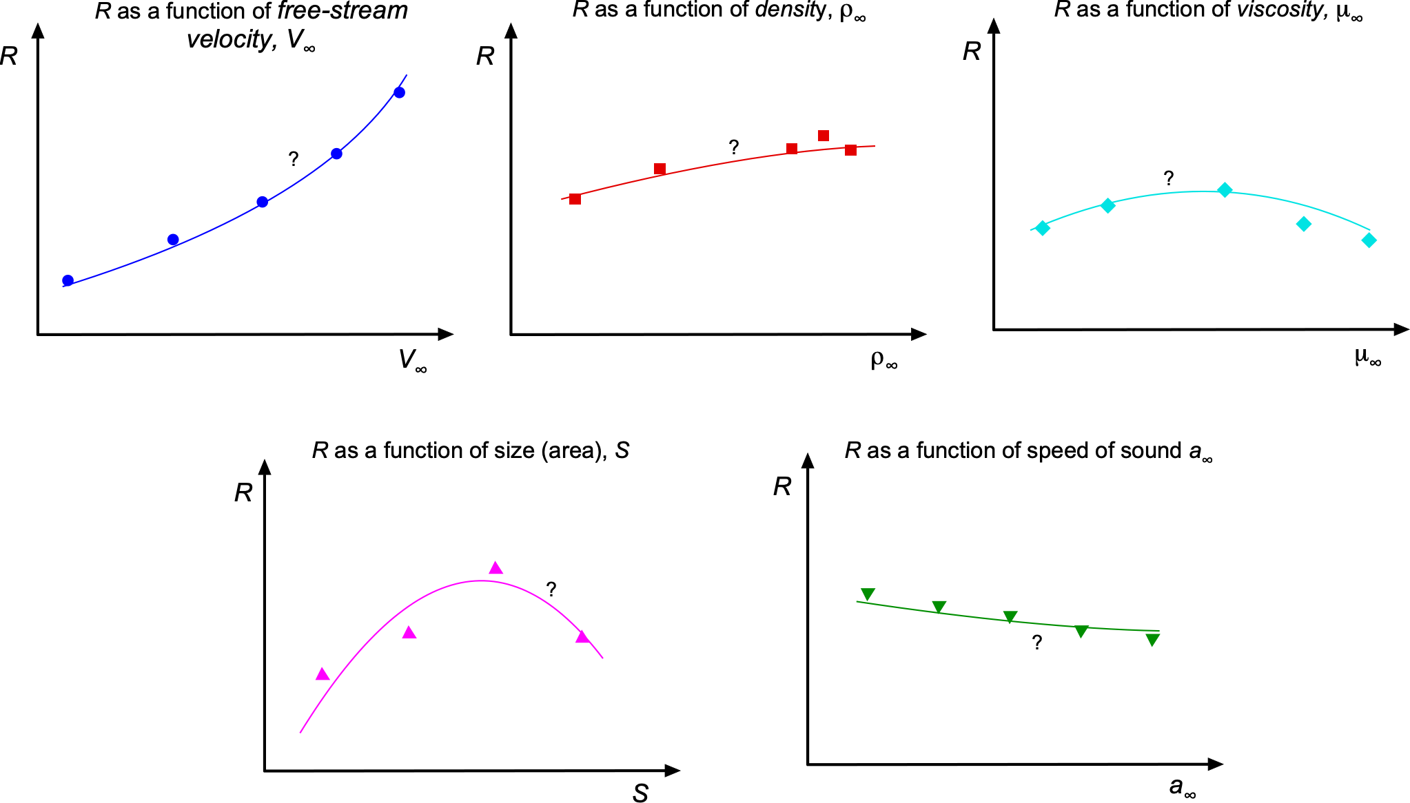
Among these variables, varying the freestream velocity,  , is straightforward in most wind tunnel facilities. Additionally, different geometrically scaled wings could be tested to investigate the effects of changing wing area,
  . However, directly controlling or systematically varying the other parameters such as air density , viscosity
  , and speed of sound
  , is significantly more challenging, if not impossible in some cases. Furthermore, isolating the effect of a single parameter while keeping all others constant presents additional difficulties. However, for the sake of this discussion, assume that such control is achievable.
Denote the number of values each parameter can take as follows:  for the first parameter,
  for the second parameter,
  for the third parameter,
  for the fourth parameter, and
  for the fifth parameter. Then, the total number of test cases is given by the product of the number of values each parameter can take will be
(3) 
For example, if each parameter is varied at only five different values, the total number of test cases would be
(4) 
Most would agree that this is a substantial number of tests to conduct in a wind tunnel! Eventually, the relationships required between and all dependent quantities at each angle of attack would be determined. If ten angles were selected, the total number of runs would exceed 30,000. Thus, it quickly becomes evident that systematically varying each dependent parameter while holding the others constant would require significant time in the wind tunnel.
This approach would also generate an extensive dataset, from which cross-plotting and possibly curve-fitting could be used to determine the functional relationships describing how , , etc., influence . If only a single independent variable were considered, the relationship could be easily represented with two columns of numbers. However, managing the data would require extensive tables or multiple pages of charts and graphs when dealing with four or more independent variables. Hence, the student soon realizes that handling an engineering problem involving three, four, or more independent variables is exceptionally challenging.
Basis of Dimensional Analysis
It is clear that systematically varying each independent parameter to establish the “cause and effect” on the dependent parameter would be impractical from a measurement perspective, nor would it be attractive from a computational (modeling) approach. Fortunately, the approach to the preceding problem can be simplified by employing dimensional analysis, which can be used to determine sets of dimensionless groups of parameters that affect the problem of interest. Such an approach will also be shown to reduce the number of independent variables, thereby becoming an essential technique for understanding many engineering problems, not just aerodynamics.
Dimensional Homogeneity
Dimensional analysis is based on the fact that if an equation of parameters such as
(5) 
expresses some physical relation, then the parameters  ,
,  ,
,  , and
, and  must all have the same dimensions and so be dimensionally homogeneous for the equation to be mathematically valid, e.g., , , , and could all be values of pressures or velocity components. Equation 5 can also be made dimensionless by dividing through by one of the terms, i.e., the same result can be expressed as
(6) 
or that
(7) 
Another advantage of this latter dimensionless form is that all quantities are now expressed as dimensionless ratios, so the system of units is irrelevant.
Complete and Incomplete Equations
An equation arising from a physical problem is said to be complete if stated so that the physical dimensions of each variable involved can be explicitly recognized. Consider a falling body accelerating to some velocity, , under gravity,  , from an initial velocity,
  . The governing equation is
(8) 
where  is the vertical distance. The form of this equation is said to be complete. However, if the equation is written as
(9) 
then it is incomplete because the dimensions of the second term in the equation cannot be recognized, i.e., it is impossible to positively conclude that 19.62 equals  . However, that would certainly be a good guess with SI units ( = 9.81 m/s2).
A parameter placed inside a set of square brackets [ ] means the dimensions of that parameter. If the equation is complete, then it is possible to conclude that in terms of dimensions, then
(10) ![\begin{equation*} {\left[ V^2 \right] = \left[ U^2 \right] = \left[ 2 \, g \, s \right]} \end{equation*}](https://eaglepubs.erau.edu/app/uploads/quicklatex/quicklatex.com-98086b59daa5217bd0988c800e9fafb1_l3.svg "Rendered by QuickLaTeX.com")
Inserting the base dimensions for each parameter gives
(11) 
and the equation is, therefore, dimensionally homogeneous.
Furthermore, to make sense of any equation, each parameter must be expressed numerically in the same units system, i.e., either entirely in SI units or entirely in USC units, in each case with the same base dimension. However, notice that Eq. 8 can also be written in non-dimensional form as
(12) 
so the system of units (SI or USC) does not matter. When undertaking derivations and developing equations in engineering, it is often desirable to work in non-dimensional forms if possible.
Satisfying Dimensional Homogeneity
As an example of dimensional homogeneity, consider the kinetic energy,  , of a mass,
  , traveling at velocity, , which is given by
(13) 
Dimensional homogeneity requires this equation to be dimensionally balanced. On the left-hand side, the units are energy, which is the ability to do work so
(14) ![\begin{equation*} \left[ KE \right] \equiv \mbox{Force times distance} = (\rm M L T^{-2} ) L = \rm M L^2 T^{-2} \end{equation*}](https://eaglepubs.erau.edu/app/uploads/quicklatex/quicklatex.com-f7d8830f5613c77e1882c87c0a018dc1_l3.svg "Rendered by QuickLaTeX.com")
On the right-hand side, then
(15) ![\begin{equation*} \left[ \frac{1}{2} m V^2\right] \equiv \mbox{Mass times velocity squared} = \rm M (L T^{-1})^2 = M L^2 T^{-2} \end{equation*}](https://eaglepubs.erau.edu/app/uploads/quicklatex/quicklatex.com-fd1cfb48defa5739c03873ab607b975c_l3.svg "Rendered by QuickLaTeX.com")
Therefore, the dimensions on the left side of this equation balance those on the right side, so the equation is dimensionally homogeneous.
Consider another problem in which dimensional homogeneity must be satisfied. To describe the fluid flow between two moving plates, the shear stress, , is some function of the viscosity,  , and the velocity difference
  between the two plates separated by a distance
  . The relationship can be expressed as
(16) 
By satisfying dimensional homogeneity, it is possible to determine the values of ,  , and
, and  . In terms of the dimensions, then
(17) ![\begin{equation*} \left[ \tau \right] = \left[ \mu \right]^{\alpha} \left[ \Delta V\right]^{\beta} \left[ h \right]^{\gamma} \end{equation*}](https://eaglepubs.erau.edu/app/uploads/quicklatex/quicklatex.com-55a1860f1032e92273d570b5c1b59df1_l3.svg "Rendered by QuickLaTeX.com")
and so for each parameter, then
(18) ![\begin{equation*} \left[ \tau \right] = \rm M \rm L^{-1} \rm T^{-2} \quad\quad \left[ \mu \right] = \rm M \rm L^{-1} \rm T^{-1} \quad\quad \left[ \Delta V \right] = \rm L \rm T^{-1} \quad\quad \left[ h \right] = \rm L \end{equation*}](https://eaglepubs.erau.edu/app/uploads/quicklatex/quicklatex.com-b56e37eb4e4b5ce3dcc318cbb5de2e35_l3.svg "Rendered by QuickLaTeX.com")
Therefore,
(19) 
To obtain dimensional homogeneity, then
(20) 
so  ,
,  , and
, and  . Inserting the values gives the final relationship as
(21) 
showing that the shear stress is proportional to the velocity gradient, with the constant of proportionality being the value of viscosity, . This equation is called Newton’s law of viscosity.
The Buckingham Π Method
These ideas of dimensional analysis and dimensional homogeneity are fundamental and intrinsic to the Buckingham  method. Lord Rayleigh and Joseph Bertrand initially set down these preceding simple, but profoundly important, principles in what is called the “Method of Dimensions.” However, these principles are now formally embodied in what is known as the “Buckingham theorem” after Edgar Buckingham, who developed it into a more structured form suitable for general use. The Buckingham Theorem (usually just called the Buckingham method or just the method) is a generalized formalization of the method of dimensions, which can now be examined. The original publication by Edgar Buckingham, a scientist at NIST, is available, which is worth reading in conjunction with the following exposition of his method.
Let  , represent a list of
  physical variables in the general physical relationship
(22) 
where  is the dependent parameter and
  are the -1 independent parameters. The function represents a general functional relationship, as yet unknown. Notice that the previous equation can also be written in an implicit form as
(23) 
where  represents another functional relationship between the parameters yet to be determined.
Let  equal the number of fundamental dimensions required to collectively describe the physical variables. In engineering, most physical variables can be expressed as a combination of mass, length, time, and temperature, so generally,
  . In mechanics, then mass, length, and time are involved, so
  . The Buckingham method then states that the relationship in Eq. 23 may be expressed as a relationship of fewer
  dimensionless products called products, where each product is a dimensionless product of a selected set of repeating variables plus one other variable. Therefore, one key to applying the method is selecting the most suitable set of repeating variables.
To see how the method works, let  be the selected repeating variables. The repeating variables are not unique in most cases, but their selection is not arbitrary and must be selected according to some specific rules. The primary and most important rule is that the selected repeating variables cannot include the dependent variable,
  , which can only appear in one of the groups. Therefore,
(24) ![\begin{eqnarray*} \Pi_{1} & = & \phi_{1} \left( \underbrace{ P_{2}, \, P_{3}......P_{K+1}}_{\mbox{~\scriptsize Repeating}} ,\underbrace{P_{1}}_{\mbox{~\scriptsize Dependent}} \right) \\[6pt] \Pi_{2} & = & \phi_{2} \left( \underbrace{ P_{2}, \, P_{3}, .....P_{K+1}}_{\mbox{~\scriptsize Repeating}} ,\underbrace{P_{K+2}}_{\mbox{~\scriptsize Other}} \right) \\[6pt] & & \bigcdot \\[6pt] & & \bigcdot \\[6pt] & & \bigcdot \\[6pt] \Pi_{N-K} & = & \phi_{N-K} \left( \underbrace{ P_{2}, \, P_{3}, .......P_{K+1}}_{\mbox{~\scriptsize Repeating}}, \underbrace{P_{N}}_{\mbox{~\scriptsize Remaining}} \right) \end{eqnarray*}](https://eaglepubs.erau.edu/app/uploads/quicklatex/quicklatex.com-3e3d2106802f842377d3f3ab05f162c3_l3.svg "Rendered by QuickLaTeX.com")
where  is the last remaining variable.
Notice that there are now  new functional relationships, i.e.,
  ,
,  ….
…. , but they are expressed in terms of the dimensionless products. Therefore, it can be written that
(25) 
where  is the functional relationship (still to be determined), it is now expressed in terms of each of the products. The functional relationship is often found from experiments, as the figure below suggests. The process of dimensional analysis does not allow theoretical relationships to be developed, i.e., equations. Notice that in explicit form, this latter equation can also be written as
(26) 
where  is some other functional relationship.
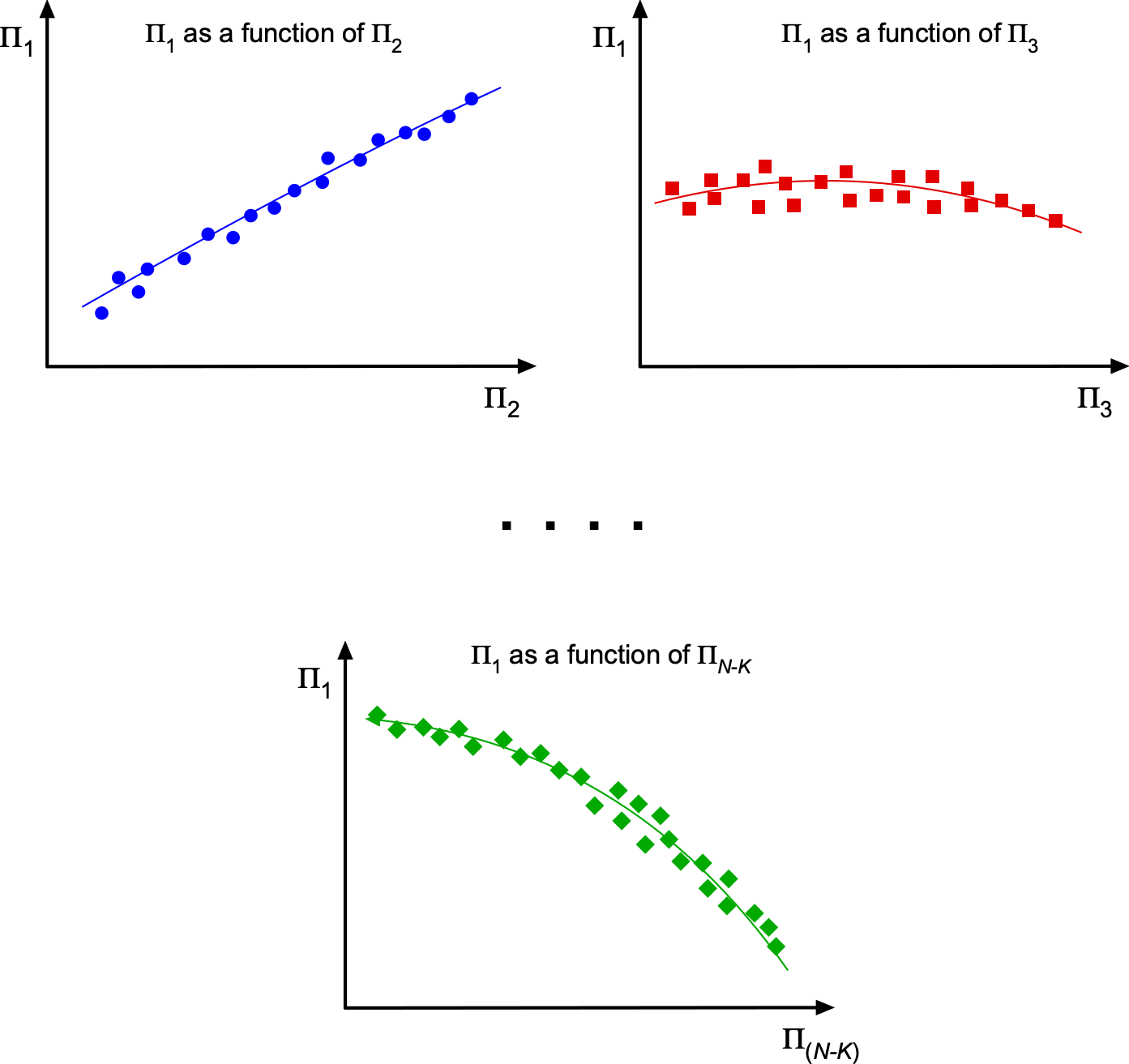
The upshot of the dimensional analysis process means that the functional relationship has been reduced from the initial dimensional variables to  dimensionless variables. Therefore, decreasing the number of dependent parameters significantly simplifies the analysis of the original problem. For example, suppose originally
  and
and  , i.e., the dependent variable is a function of five other parameters as in the aforementioned wing problem. In that case, the dimensional analysis will reduce the problem to three dimensionless groupings, i.e., one dimensionless grouping becomes a function of two other dimensionless groupings. If
  and , then the dimensional analysis will reduce the problem to two dimensionless groupings in that one grouping becomes a sole function of the other grouping. The potential simplifications, therefore, that can be afforded by dimensional analysis become clear.
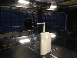
Π Method Applied to the Drag on a Sphere
Consider a sphere to be tested in a low-speed wind tunnel to measure its drag, as shown in the photograph below. The drag of a sphere sounds relatively uninteresting compared to a wing, but this problem helps introduce the dimensional analysis process without making the process too lengthy. Furthermore, the aerodynamic characteristics of a sphere are particularly relevant to all sorts of ball games, such as tennis, baseball, soccer, and many others. The motion of balls through the air is a complex fluid dynamic problem that is influenced by many factors, including the flow density and viscosity, the velocity and size of the ball, and its surface finish. For example, the aerodynamics of a golf ball affects the distance, spin, and overall trajectory of the ball. Ever wonder why a golf ball has dimples on its surface? In baseball, the aerodynamics of the ball can influence the speed and trajectory of a pitch.
Functional Dependency
The objective is to find the dimensionless groupings describing this aerodynamic problem. On a physical intuitive basis, the aerodynamic drag force,  , on the sphere would be expected to depend on:
- Free-stream velocity, .
- Free-stream density, .
- Free-stream viscosity, i.e., the coefficient of viscosity .
- The size of the sphere, as described by its diameter
 .
.
This list may be incomplete, and other parameters may affect the drag, such as surface roughness and speed of sound. On the one hand, omitting a relevant parameter may restrict the validity of the result or make it wrong. On the other hand, including unnecessary parameters may make the final result more complicated than it should be.
The relationship between and the air properties may be written in a general functional form as
(27) 
The drag is the dependent variable. , , and are the independent variables. In this case, the functional dependence is denoted by .
Following the Buckingham method, the functional dependence is then written in implicit form, i.e.,
(28) 
where is some other function. In this case, , ,  , so there are two products to be determined.
Understanding explicit versus implicit functional forms
What is the difference between writing an equation  and the form
  ? In mathematics, the dependent function, say
  , for example, can be written in terms of other parameters, e.g., where
  is some function, or more generally as
  , which are called explicit functional dependencies. However, the relationship can also be written in implicit form, i.e., is equivalent to
  . Notice that the function
  is NOT the same as the function . If
  , for example, then , which is an explicit dependency of
  on
on  . Alternatively, it can be written that
  , which is in the form , which is the implicit form of the same relationship. Likewise,
  as
as  . In dimensional analysis, the process starts by writing the functional dependency of the problem parameters in implicit form.
Dimensions of the Variables
Now, the dimensions of the variables in this problem must be determined. Remember that the square brackets [-] around a variable means “the dimensions of” that variable. For each dependency, then
(29) ![\begin{eqnarray*} \left[ D \right] & = & \rm M L T^{-2} \\ \left[ \varrho_{\infty} \right] & = & \rm ML^{-3} \\ \left[ V_{\infty} \right] & = & \rm LT^{-1} \\ \left[ \mu_{\infty} \right] & = & \rm ML^{-1} \rm T^{-1} \\ \left[ d \right] & = & \rm L \end{eqnarray*}](https://eaglepubs.erau.edu/app/uploads/quicklatex/quicklatex.com-f3279d927b71b07cc902bac6e72343e8_l3.svg "Rendered by QuickLaTeX.com")
Recall that the dimensions of force are obtained from mass times acceleration, i.e., MLT.
Dimensional Matrix
The solution to the dimensional analysis problem proceeds by setting up a dimensional matrix with all the parameters in their base dimensions. Setting up the dimensional matrix, in this case, gives
(30) 
One purpose of the dimensional matrix is to lay the problem out clearly and test for the linear independence of the repeating variables in terms of the chosen primary dimensions.
Repeating Variables
Although the selection of the repeating variables can be viewed as somewhat arbitrary, in general, they must always be selected based on four essential rules:
- The repeating variables must all have a primary dependency on the dependent variable. In this case, the variables
 and can all be expected to have strong effects on the dependent variable, .
 - The dependent variable, , cannot be used as a repeating variable, so it must appear only in one group by default. No exceptions.
- The repeating variables must include all of the physical base dimensions of the problem, i.e., they must collectively include mass and/or length and/or time, as appropriate, for the particular problem in question. In this case, , and collectively include the base dimensions of mass, length, and time.
- The repeating variables must be linearly independent of one another, i.e., repeating variables must not be chosen that will have the same units or products of the same units, e.g., repeating variables with two different length scales or two different reference velocities cannot be used. In addition, repeating variables that are already dimensionless or repeating variables that can form a dimensionless group by themselves will not be linearly independent of each other. In this case, , and are all linearly independent of each other.
The dimensional analysis process will likely succeed if these prior rules are followed. If not, then it will fail, often catastrophically. The choice of repeating variables may not be obvious for complex problems, for which there are many in engineering! However, they should still be selected as quantities most likely to have substantial effects on the dependent variable. For example, the velocity and density of the flow in an aerodynamic problem are two quantities that will significantly affect the aerodynamic forces.
Formal Check for Linear Independence
To formally check for linear independence (although, in most cases, this will be obvious), the determinant of the sub-matrix formed by the selected repeating variables must be determined, which in this case is
(31) 
If  ,
,  , and
, and  are non-zero constants in the following equation for linear independence, then
(32) ![\begin{equation*} c_1 \left[ \begin{array}{r} 1 \\ -3 \\ 0 \end{array} \right] + c_2 \left[ \begin{array}{r} 0 \\ 1 \\ -1 \end{array} \right] + c_3 \left[ \begin{array}{r} 0 \\ 1 \\ 0 \end{array} \right] \ne 0 \end{equation*}](https://eaglepubs.erau.edu/app/uploads/quicklatex/quicklatex.com-02b86e14fcfee461ee4f697643621b47_l3.svg "Rendered by QuickLaTeX.com")
Reassembling this in matrix form gives
(33) ![\begin{equation*} \left[ \begin{array}{rrr} 1 & 0 & 0 \\ -3 & 1 & 1 \\ 0 & -1 & 0 \end{array} \right] \left[ \begin{array}{r} c_1 \\ c_2 \\ c_3 \end{array} \right] \ne 0 \end{equation*}](https://eaglepubs.erau.edu/app/uploads/quicklatex/quicklatex.com-0a790223966cdd554661c60eb55be778_l3.svg "Rendered by QuickLaTeX.com")
For this matrix equation to have a nontrivial solution, then the determinant must be non-zero, i.e., the test in this case is whether
(34) ![\begin{equation*} \det \left[ \begin{array}{rrr} 1 & 0 & 0 \\ -3 & 1 & 1 \\ 0 & -1 & 0 \end{array} \right] \equiv \left| \begin{array}{rrr} 1 & 0 & 0 \\ -3 & 1 & 1 \\ 0 & -1 & 0 \end{array} \right| \ne 0 \, ? \end{equation*}](https://eaglepubs.erau.edu/app/uploads/quicklatex/quicklatex.com-af1dccef78c7a290f1d7ab4df1267b74_l3.svg "Rendered by QuickLaTeX.com")
Therefore, the determinant is
(35) 
Therefore, it has now been formally verified that the selected repeating variables and are indeed linearly independent of each other. In most cases, however, the formal test is not needed because if the variables are chosen such that they do not have the same units or products of the same units, then they will be linearly independent.
Development of the Π Products
Following the Buckingham method, then the products in this case will be
![\begin{eqnarray*} \Pi_{1} & = & \phi_{1} \left( \underbrace{\varrho_{\infty}, \, V_{\infty}, \, d}_{\mbox{~\scriptsize Repeating}} , \underbrace{D}_{\mbox{~\scriptsize Dependent}} \right) \\[8pt] \Pi_{2} & = & \phi_{2} \left( \underbrace{\varrho_{\infty}, \, V_{\infty}, \, d}_{\mbox{~\scriptsize Repeating}} , \underbrace{\mu_{\infty}}_{\mbox{~\scriptsize Remaining}} \right) \end{eqnarray*}](https://eaglepubs.erau.edu/app/uploads/quicklatex/quicklatex.com-711a0aaa318c1245b9a48bf87f2e49ae_l3.svg "Rendered by QuickLaTeX.com")
First Π Product
For  then
then
(36) 
The values of the coefficients , , and must now be obtained to make the equation dimensionally homogeneous and dimensionless. In terms of the dimensions of the parameters, then
(37) ![\begin{equation*} \left[ \Pi_{1} \right] = 1 = \rm M^{0}L^{0}T^{0} = \left( \rm ML^{-3} \right)^{\alpha} \left( LT^{-1} \right)^{\beta} \left( \rm L \right)^{\gamma} \left( \rm MLT^{-2} \right) \end{equation*}](https://eaglepubs.erau.edu/app/uploads/quicklatex/quicklatex.com-4f52ef8db851574a3364408be69b41d7_l3.svg "Rendered by QuickLaTeX.com")
Because the left-hand side of the above equation is dimensionless, it means that the powers or exponents of M, L, and T must add to zero to make the equation dimensionally homogeneous and dimensionless. Therefore, for to be dimensionless, then
(38) 
so that

By inspection,  ,
,  , and
, and  . Therefore, the first product is
(39) 
or
(40) 
which is a force coefficient. Usually, aerodynamic force coefficients are defined in terms of the dynamic pressure, i.e.,  . Also, in this case, a good reference is to use projected area
  . Therefore, the force coefficient would be written as
(41) 
It is always good to check the final dimensions of the grouping to be sure it is dimensionless, i.e., it has dimensions of 1. So, in this case
(42) ![\begin{equation*} \left[ C_D \right] = \frac{\rm M L T^{-2}}{ (\rm M L^{-3}) (\rm L^2 T^{-2}) (L^{2})} = \frac{\rm M L T^{-2}}{\rm M L T^{-2}} = 1 \end{equation*}](https://eaglepubs.erau.edu/app/uploads/quicklatex/quicklatex.com-f87d42d9c939ab9bb43b10ad5ad3d6ef_l3.svg "Rendered by QuickLaTeX.com")
which confirms that the grouping is dimensionless.
Dealing with exponents or powers
In dimensional analysis, solving for the dimensionless groupings involves adding the values of the unknown exponents for each base dimension. Exponents are also called the power of the quantity because they represent the number of times a quantity is multiplied by itself. Here are some examples:
![\[\small 2^2 \, 2^3 = 2^{2+3} = 2^5 \]](https://eaglepubs.erau.edu/app/uploads/quicklatex/quicklatex.com-696146ae6a2ecbdb56841f73b112acf0_l3.svg "Rendered by QuickLaTeX.com")
![\[ x^a \, x^b = x^{a+b} \]](https://eaglepubs.erau.edu/app/uploads/quicklatex/quicklatex.com-112d433712fa81d22a2f184d78f0d1d4_l3.svg "Rendered by QuickLaTeX.com")
![\[ x^a \, y^b \, y^c = x^a \, y^{b+c} \]](https://eaglepubs.erau.edu/app/uploads/quicklatex/quicklatex.com-8782a723f104a0f5312c94b5002c49fe_l3.svg "Rendered by QuickLaTeX.com")
![\[ \rm M^{\alpha} \, \rm M^{\beta + 1} = \rm M^{(\alpha + \beta + 1)} \]](https://eaglepubs.erau.edu/app/uploads/quicklatex/quicklatex.com-db64caa0877d286d80622178509670ae_l3.svg "Rendered by QuickLaTeX.com")
![\[ \rm M^{\alpha} \, \rm L^{\gamma} \, \rm M^{\beta -2 } \, L^{-1} = \rm M^{(\alpha + \beta - 2)} \, \rm L^{\gamma -1} \]](https://eaglepubs.erau.edu/app/uploads/quicklatex/quicklatex.com-4626a67a82fc8e48de209e774b9d71c5_l3.svg "Rendered by QuickLaTeX.com")
When working with exponents, remember that the base parameter has to be the same, and the addition is performed on the exponent.
Second Π Product
For  then
then
(43) 
so, in terms of dimensions, then
(44) 
Equating the powers gives

Therefore, in this case ,  , and .
(45) 
i.e.,
(46) 
Or by inverting the quantity, a dimensionless grouping is still obtained, i.e.,
(47) 
Remember from before that this dimensionless parameter is called the Reynolds number. Again, a check should be made to be sure that the grouping is dimensionless, so in this case
(48) ![\begin{equation*} \left[ Re \right] = \frac{(\rm M L^{-3}) ( \rm L T^{-1}) (\rm L) }{ \rm M L^{-1} T^{-1}} = \frac{\rm M L^{-1} \rm T^{-1} }{ \rm M L^{-1} T^{-1}} = 1 \end{equation*}](https://eaglepubs.erau.edu/app/uploads/quicklatex/quicklatex.com-9e2782c2cfbbabe0268af0a50ecd0251_l3.svg "Rendered by QuickLaTeX.com")
which indeed confirms that the grouping is dimensionless.
Final Result for Functional Dependency
As a result of the dimensional analysis of the sphere, then
(49) 
or
(50) 
In explicit form, the relationship between the drag coefficient and the Reynolds number is
(51) 
So, now, instead of the drag being a function of four parameters, i.e.,
(52)
the drag coefficient is a function of one non-dimensional parameter, i.e.,
(53)
Benefits of Dimensional Analysis
The benefits of dimensional analysis have now become much clearer. In this latter problem of finding the effects of different parameters on the drag of a sphere, the question for the analyst comes down to finding the explicit relationship between drag and four parameters versus finding the relationship between a force coefficient and the Reynolds number, as summarized in the figure below. Most analysts would side with the latter approach, not only because it involves less work but because the results from other experiments and at different Reynolds numbers, such as in other wind tunnels, can be directly compared on the same non-dimensional basis.
Dimensional analysis is also essential for generalizing data and establishing causal relationships, including for design purposes. In general, dimensional analysis provides a systematic approach for consistency checking, unit conversion, estimation, modeling, experimental design, equation verification, and problem-solving across various engineering and scientific disciplines.
The original dimensional analysis paper by Edgar Buckingham.
The original dimensional analysis paper by Edgar Buckingham dates to 1914. Notice his comments on dealing with the square root of parameters (“dispense with fractional exponents”), the choice of repeating variables, and the inversion of dimensionless groupings. Later in the paper, he talks about the “screw propeller” problem and dynamic similarity, which he recognizes as a powerful tool for scaling measurements made on models and relating them to full scale. In 1914, he commented, “This subject seems to be less familiar to physicists than it deserves to be…” Today, we take advantage of dimensional analysis and the principles of dynamic similarity in much of what we do as engineers. It sometimes pays to step back and remember how we got this far.
Doing the Experiment
The functional dependency to be measured is now  . The drag force on the sphere, , can be measured with a balance and with measurements of the flow velocity , as well as density, , and viscosity , (via measurements of pressure and temperature), calculations are made of:
1. The drag coefficient, 
2. The Reynolds number, 
The figure below shows the results for the sphere’s drag coefficient as measured in the wind tunnel as a function of Reynolds number. The data collection can proceed rapidly because the values of the groupings are being plotted rather than the values of the individual parameters. Notice the rapid decrease in the drag coefficient between  and
and  , which suggests that something very profound is happening to the flow about the sphere. Indeed, this behavior is tied to the flow characteristics on the sphere’s surface, called the boundary layer, and how the flow separates behind the sphere and creates a wake. In this dimensionless form, these results can also be directly compared to measurements made, for example, in another wind tunnel or added to a pool of data covering other ranges of Reynolds numbers.
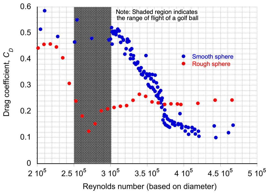
Effects of surface roughness?
Notice also from the results given in the preceding plot that the sphere’s drag coefficient depends on whether the sphere has a smooth or rough surface. Indeed, this is a very interesting outcome as it affects the drag of a golf ball. Therefore, it is helpful to think about what might happen if surface roughness was added as the fifth variable to the parameter list, i.e., in this case, assume that
![\[ D = \phi \left( \varrho_{\infty}, V_{\infty}, \mu_{\infty}, d , \epsilon \right) \]](https://eaglepubs.erau.edu/app/uploads/quicklatex/quicklatex.com-6d6547346ed44d2dd1f51520ece41ac4_l3.svg "Rendered by QuickLaTeX.com")
where  is a linear measure of the roughness height. The new functional dependence of in the implicit form is
![\[ \psi\left( \varrho_{\infty}, \, V_{\infty}, \, \mu_{\infty}, \, d, \, \epsilon, \, D \right) = 0 \]](https://eaglepubs.erau.edu/app/uploads/quicklatex/quicklatex.com-d5aa9051595ad6704350c50ab6fc825b_l3.svg "Rendered by QuickLaTeX.com")
In this case, , ,  , so there are three products. The first two products have already been determined, and it is easily shown that now
![\[ C_{D} = \phi_3 \left( Re , \frac{\epsilon}{d} \right) \]](https://eaglepubs.erau.edu/app/uploads/quicklatex/quicklatex.com-510ec5c2f5e317c429df159a51b943ad_l3.svg "Rendered by QuickLaTeX.com")
where  is a dimensionless roughness height. Notice that the effects of roughness decrease the drag of a sphere in the range where golf balls fly, which allows them to go further.
Π Method Applied to a Wing
Returning to the wing problem initially discussed, the explicit dependency of the resultant aerodynamic force (the dependent quantity) in terms of the independent variables is
(54) 
The functional dependence can also be written in implicit form, i.e.,
(55) 
where is some functional dependency to be determined. Following the method then , , , and so three products must be found in this case.
Dimensions of the Variables
Now, the dimensions of the variables must be determined. For each dependency in this case, then
(56) ![\begin{eqnarray*} \left[ R \right] & = & \rm MLT^{-2} \\ \left[ \varrho_{\infty} \right] & = & \rm ML^{-3} \\ \left[ V_{\infty} \right] & = &\rm LT^{-1} \\ \left[ S \right] & = & \rm L^2 \\ \left[ \mu_{\infty} \right] & = & \rm ML^{-1}T^{-1} \\ \left[ a_{\infty} \right] & = & \rm LT^{-1} \end{eqnarray*}](https://eaglepubs.erau.edu/app/uploads/quicklatex/quicklatex.com-473e76cbceaeed609685994836491805_l3.svg "Rendered by QuickLaTeX.com")
Notice that the dimensions of force are obtained from the product of mass and acceleration, i.e., [] =  . It is critically important that each variable is assigned the correct base dimensions. If not, the Buckingham method will fail.
Forming the Dimensional Matrix
The solution to the dimensional analysis problem proceeds by setting up a dimensional matrix with all of the parameters being given in terms of their base dimensions, i.e.,
(57) 
Choice of Repeating Variables
In this problem, a good choice of the repeating variables is , and , which is a common choice for aerodynamic problems. Remember not to choose the dependent variable as a repeating variable. Remember also that the repeating variables must be linearly independent, i.e., the dimensions of any one repeating variable cannot be linearly obtained from the dimensions of any other. Choosing repeating variables with different dimensions or products of dimensions is necessary. For example, two repeating variables comprising a length and an area or two repeating variables with units, cannot be used, or the method will fail. Furthermore, the repeating variables must collectively include all of the base dimensions of the problem.
In this case, the choice of the repeating variables , and satisfy all of these requirements. This can also be confirmed by determining the determinant of the dimensional submatrix in Eq. 57 that is formed by the repeating variables, which shows that
(58) 
IMPORTANT! Rules for choosing the repeating variables
The formal determination that the repeating variables are linearly independent takes some work, although it is just arithmetic. However, in some cases, this outcome can be verified by inspection. Some basic rules can help choose the repeating variables, so the formal test for linear independence can be foregone. These rules are:
- NEVER choose the dependent variable as a repeating variable! If this rule is ignored, then the Buckingham method will fail catastrophically.
- Always choose repeating variables that will, or are likely to, have a primary effect on the dependent variable. For aerodynamic problems, these are usually the density of the flow, the speed of the flow, and some area or length scale.
- Do NOT choose repeating variables that have the same dimensions, so don’t choose two repeating variables, such as flow velocity and the speed of sound (which both have dimensions of length/unit time), or two length variables, such as a wing chord and a wing span (both have dimensions of length). Furthermore, two variables with dimensions of length and area, respectively, cannot be used as repeating variables because they are also not linearly independent.
- Remember that the choice of repeating variables may not, in most cases, be unique! The choice is not arbitrary, but a different choice of repeating variables will inevitably lead to a different set of dimensionless groupings. Even though dimensionless groupings are obtained, the process can be conducted again with a different set of repeating variables.
Development of the Π Products
Continuing to follow the Buckingham procedure, then the products in this problem are
(59) ![\begin{eqnarray*} \Pi_{1} & = & \phi_{1} \left( \underbrace{\varrho_{\infty}, V_{\infty}, S}_{\mbox{~\scriptsize Repeating}} , \underbrace{R}_{\mbox{\scriptsize ~Dependent}} \right) \\[8pt] \Pi_{2} & = & \phi_{2} \left( \underbrace{\varrho_{\infty}, V_{\infty}, S}_{\mbox{~\scriptsize Repeating}} , \underbrace{\mu_{\infty}}_{\mbox{~\scriptsize Other}} \right) \\[8pt] \Pi_{3} & = & \phi_{3} \left( \underbrace{\varrho_{\infty}, V_{\infty}, S}_{\mbox{~Repeating}} , \underbrace{a_{\infty} }_{\mbox{~\scriptsize Remaining}}\right) \end{eqnarray*}](https://eaglepubs.erau.edu/app/uploads/quicklatex/quicklatex.com-3174d1ed77ddec456c099987a6bc6773_l3.svg "Rendered by QuickLaTeX.com")
First Π Product
Take the first product, , then
(60) 
where the coefficients , , and are unknowns, and their values must be obtained appropriately to make the equation dimensionally homogeneous, i.e., finding their values to make the equation dimensionless with dimensions of 1. In terms of the dimensions, then
(61) ![\begin{equation*} \left[ \Pi_{1} \right] = \rm M^{0}L^{0}T^{0} = \left( \rm ML^{-3} \right)^{\alpha} \left(\rm LT^{-1} \right)^{\beta} \left( \rm L^2 \right)^{\gamma} \left( MLT^{-2} \right) \end{equation*}](https://eaglepubs.erau.edu/app/uploads/quicklatex/quicklatex.com-d3e141531cdf8c83d5f61450f99942d2_l3.svg "Rendered by QuickLaTeX.com")
where ![\left[x\right]](https://eaglepubs.erau.edu/app/uploads/quicklatex/quicklatex.com-26842f64ee88a7dad480c09046136cc0_l3.svg "Rendered by QuickLaTeX.com") is used to mean “the dimensions of variable
is used to mean “the dimensions of variable  .” Collecting the terms gives
(62) ![\begin{equation*} \left[ \Pi_{1} \right] = \rm M^{0}L^{0}T^{0} = \rm M^{(\alpha+1)} \, \rm L^{(-3\alpha+\beta+2\gamma+1)} \, \rm T^{(-\beta-2)} \end{equation*}](https://eaglepubs.erau.edu/app/uploads/quicklatex/quicklatex.com-89f42a9ce1d876dbc8142fb9c33eec8d_l3.svg "Rendered by QuickLaTeX.com")
Because the left-hand side of the above equation is dimensionless, it means that the powers or exponents of M, L, and T must add to zero to make the equation dimensionally homogeneous, i.e.,
(63) 
Therefore, in this case by inspection then , , and and so the first product is
(64) 
or
(65) 
Hence, is a form of force coefficient. Aerodynamic force coefficients are nearly always defined in terms of the dynamic pressure, i.e., , which is referred to as  , so more usually the force coefficient would be written as
(66) 
Notice that multiplying a similarity parameter by a constant value does not change the dimensions of that parameter.Paralleling the above approach used to find , the two remaining products, namely and  , can now be derived.
Second Π Product
For  then
then
(67) 
so
(68) ![\begin{equation*} \left[ \Pi_{2} \right] = \rm M^{0} L^{0} T^{0} = \left(\rm ML^{-3} \right)^{\alpha} \left( \rm LT^{-1} \right)^{\beta} \left( \rm L^2 \right)^\gamma \left( \rm ML^{-1}T^{-1} \right) \end{equation*}](https://eaglepubs.erau.edu/app/uploads/quicklatex/quicklatex.com-0dac871c52e60ec5f254cda384b963c5_l3.svg "Rendered by QuickLaTeX.com")
and
(69) 
Therefore, in this case , , and  and so this product becomes
(70) 
This derived product is a dimensionless parameter that will become infinite as the velocity tends to zero. This behavior is inconvenient, but the product can be inverted to prevent that. The outcomes are still a dimensionless parameter, but now one that is more convenient, i.e., the product becomes
(71) 
Because, in this case, there is a square root of an area, it can be replaced by a linear dimension, such as the chord of the wing , i.e., the area of a rectangular wing will be its chord times the span of the wing or  , so now
(72) 
The choice of the appropriate length scale is somewhat arbitrary (e.g., the wing span could have been used). Still, generally, in an aerodynamic problem, a parameter describing a downstream distance should be used, e.g., wing chord in this case.
This latter dimensionless parameter is known as the Reynolds number, which is denoted by the symbol  . The Reynolds number is one of the most significant parameters in aerodynamics because it governs the relative magnitude of viscous effects to inertia effects in the flow.
Third Π Product
Similarly, for the third product, then
(73) 
and so, in terms of dimensions, then
(74) ![\begin{equation*} \left[ \Pi_{3} \right] = \rm M^{0}L^{0}T^{0} = \left( \rm ML^{-3} \right)^{\alpha} \left( \rm LT^{-1} \right) ^{\beta} \left( \rm L^2 \right)^{\gamma} \left(\rm LT^{-1} \right) \end{equation*}](https://eaglepubs.erau.edu/app/uploads/quicklatex/quicklatex.com-b4dc70fa4df852159d91c60828a7507e_l3.svg "Rendered by QuickLaTeX.com")
giving
(75) 
Therefore, in this case  , , and
  , i.e.,
(76) 
Again, the product can be inverted for convenience (to put on the numerator) and still have adimensionless quantity so
(77) 
This particular dimensionless parameter is called the Mach number (the freestream Mach number in this case), which is the ratio of the freestream velocity to the freestream speed of sound. Mach number is an essential quantity in aerodynamics that affects the magnitude of the forces on a body and the general compressible nature of the flow.
Final Result for Functional Dependency
Therefore, as a result of the dimensional analysis of the wing problem, then
(78) 
or
(79) 
or in explicit form
(80) 
In dimensional form, then
(81) 
which is sometimes called Rayleigh’s equation.
The previous result is a significant outcome because it means the original aerodynamic problem in the wind tunnel has been reduced from one involving five independent variables (for which it is practically impossible to determine the functional relationships to ) to one that now only has two variables! Therefore, with a little effort, it has been shown that to determine the force on a given wing at a given angle of attack , then only the dependence of and  on need to be established. The dimensionless parameters (the Reynolds number) and (the Mach number) are known as similarity parameters.
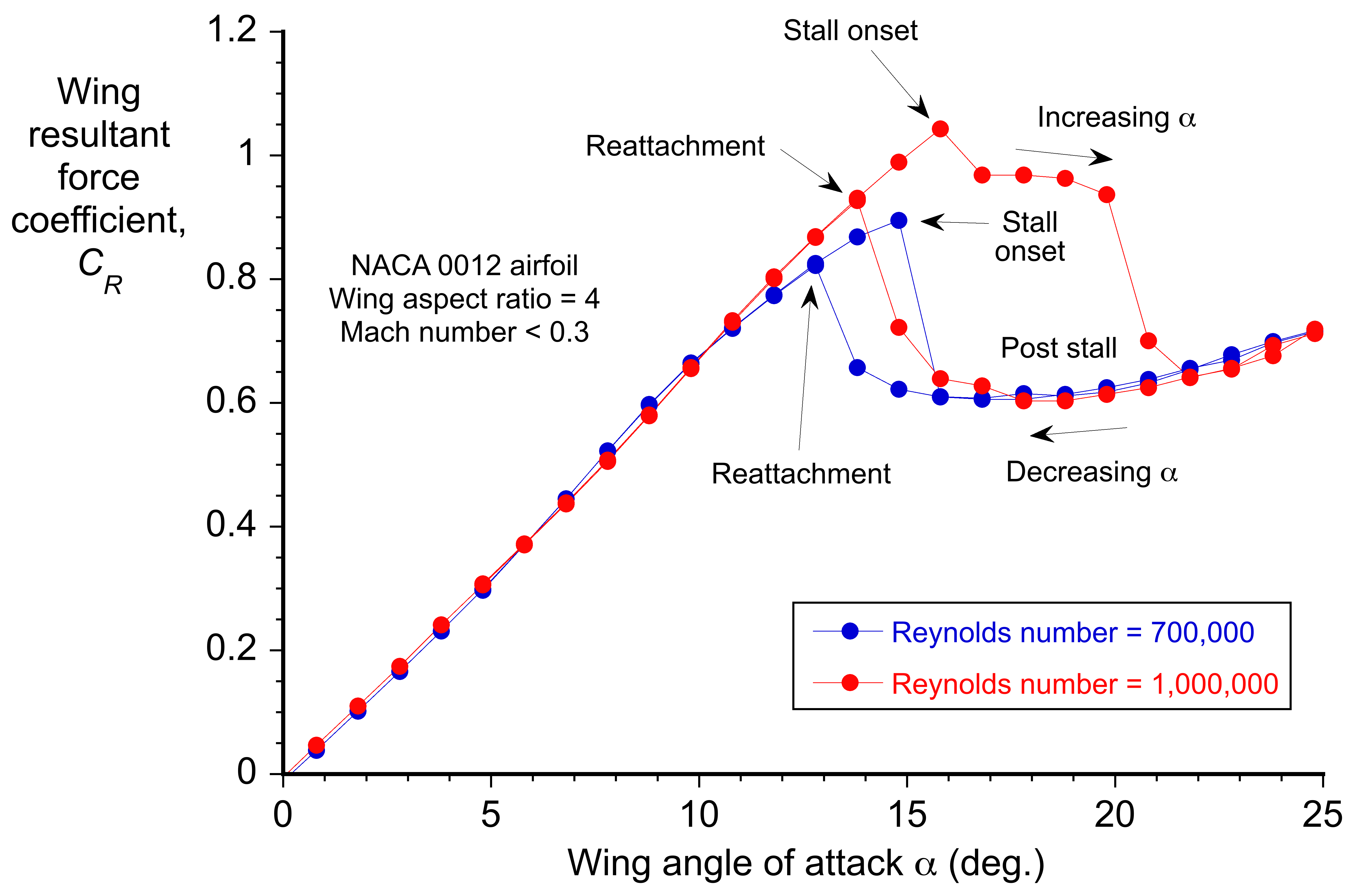
The plot below shows the actual results from the wind tunnel test to measure the resultant force coefficient,  , as a function of the wing’s angle of attack, , to the freestream flow. The measurements were performed at two different values of the Reynolds number, which in this case was obtained by varying the wind speed. Notice the significant effect of a higher Reynolds number, which increases the angle of attack and the maximum force coefficient before the onset of stall. Look carefully at the plot below. Why does the resultant force vary depending on whether the angle of attack is increasing or decreasing? In general, the values of the Reynolds and Mach numbers will substantially affect the aerodynamic forces produced on an airfoil section and on an entire wing, which is discussed in more detail in the following chapters.
Why cannot both a∞ and V∞ be chosen as repeating variables?
The answer is that they have the same units and are not linearly independent. This can be mathematically verified by finding the determinant of the dimensional matrix in this case, i.e.
![\[ \begin{array}{l|r|r|} \mbox{\small Base~unit} & a_{\infty} & V_{\infty} \\ \hline \text{\small Length, L} \quad & 1 & 1 \\ \text{\small Time, T} \quad & -1 & -1 \end{array} \]](https://eaglepubs.erau.edu/app/uploads/quicklatex/quicklatex.com-3b3c28e6eca7d5689f77bcdba22d757b_l3.svg "Rendered by QuickLaTeX.com")
The determinant of the matrix gives
![\[ \det \left[ \begin{array}{rr} 1 & 1 \\ -1 & -1 \end{array} \right] = 1 \times (- 1 ) - (-1) \times 1 = 0 \]](https://eaglepubs.erau.edu/app/uploads/quicklatex/quicklatex.com-e31d3b4e4403c1deb2935cede24b80c5_l3.svg "Rendered by QuickLaTeX.com")
Because the determinant is zero, then and are not linearly independent, and so both variables together cannot be chosen as repeating variables. As a final step, it is easy to prove that powers of parameters with the same dimensions are also not linearly independent.
Adding Wing Span to the Problem
In a final step, consider what would happen if wing span was added as a seventh variable to the parameter list in this previous problem, i.e., in this case, assume that
(82) 
Therefore,  , ,
, ,  , and so four products will result from the dimensional analysis. The first three have already been determined. It does not take much work to show that the fourth dimensionless grouping will be
(83) 
which is a span-to-chord ratio known as the aspect ratio of the wing,  . Therefore, in functional form, the resultant force can be written as
(84) 
The outcome is that by measuring the aerodynamic characteristics of a wing as a function of its aspect ratio, freestream Mach number, and Reynolds number, the wing’s behavior can be uniquely defined for any combination of flight conditions. Notice that the aspect ratio measures the slenderness of the wing. Wings that are long and narrow will have a higher aspect ratio. The results in the figure below show the effects on the resultant force on the wing by decreasing its aspect ratio from 4 to 3. This particular wing used in the wind tunnel has replaceable tip extensions to allow changes in aspect ratio and the addition of different tip shapes, including winglets. Notice that the higher aspect ratio gives a higher force for a given angle of attack. Furthermore, the drag is reduced with a higher aspect ratio wing.
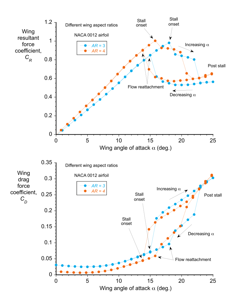
Measurements, as well as theory, show that the value of at a given Reynolds and Mach number is inversely proportional to the aspect ratio, i.e.,
(85) 
so the higher the aspect ratio, the greater the force coefficient. The theory also gives the result that the drag (induced drag) is given by
(86) 
Therefore, wings with a high aspect ratio are more efficient because for a given angle of attack, and all other parameters such as Mach number and Reynolds number being held constant, a wing with a higher aspect will produce more lift and less drag. The additional results shown in the figure below confirm the influence of the aspect ratio on the resultant force coefficient.
Practicing Exemplars
The best way of learning the method of dimensional analysis is by example. Practice first by checking and balancing equations for dimensional homogeneity to ensure the terms have the correct dimensions and units. Then, practice problems using the Buckingham method to find dimensionless groupings. After working through two or three more examples, one will quickly realize the power of dimensional analysis and how this technique can help in engineering problem-solving. Naturally, the method is not restricted to aerodynamics, and the process of dimensional analysis is helpful in all branches of engineering and the physical sciences.
Check Your Understanding #1 – Balancing equations for dimensional homogeneity
The kinetic energy, of a rotating propeller, depends on its moment of inertia,  , and its angular velocity,
  . The relationship can be expressed as
![\[ {KE = C \, I^{\alpha} \, \Omega^{\beta}} \]](https://eaglepubs.erau.edu/app/uploads/quicklatex/quicklatex.com-a92a667d7ccb12d3db1f7b88e92afe95_l3.svg "Rendered by QuickLaTeX.com")
where  is a dimensionless constant. Write down the base dimensions of each of the parameters. Then, by satisfying dimensional homogeneity, determine the values of and . Show all steps in your analysis. Hint: Moment of inertia has dimensions of mass times length squared. Show ALL steps in your analysis.
Show solution/hide solution.
We are given that
![\[ KE = C \, I^{\alpha} \, \Omega^{\beta} \]](https://eaglepubs.erau.edu/app/uploads/quicklatex/quicklatex.com-d8d5536adf574303c6d9b8491600d93a_l3.svg "Rendered by QuickLaTeX.com")
where is a dimensionless constant. In terms of the dimensions
![\[ \left[ KE\right] = \left[ I^{\alpha} \right] \left[ \Omega^{\beta} \right] \]](https://eaglepubs.erau.edu/app/uploads/quicklatex/quicklatex.com-b9626642abe7c01ae3e588325d057df7_l3.svg "Rendered by QuickLaTeX.com")
In terms of dimensions for each parameter, then
![\[ \left[ KE \right] = \rm M L^2 T^{-2} \quad\quad \left[ I \right] = \rm M L^{2} \quad\quad \left[ \Omega \right] = \rm T^{-1} \]](https://eaglepubs.erau.edu/app/uploads/quicklatex/quicklatex.com-f330cc0b07456733407755ed216752e6_l3.svg "Rendered by QuickLaTeX.com")
so
![\[ \rm M L^2 T^{-2} = \left(\rm M L^{2} \right)^\alpha \, \left( \rm T^{-1}\right)^\beta \]](https://eaglepubs.erau.edu/app/uploads/quicklatex/quicklatex.com-f793aabfefff99a16502403ab86943f5_l3.svg "Rendered by QuickLaTeX.com")
For dimensional homogeneity, then

so and  . Inserting the values gives the relationship as
![\[ KE = C \, I^{1} \, \Omega^{2} = C \, I \, \Omega^{2} \]](https://eaglepubs.erau.edu/app/uploads/quicklatex/quicklatex.com-985ce54e8beb34e5b1ae78e11e8fa77a_l3.svg "Rendered by QuickLaTeX.com")
Therefore, the final answer is
![\[ KE = C \, I \, \Omega^{2} \]](https://eaglepubs.erau.edu/app/uploads/quicklatex/quicklatex.com-cc4c7f5bad75aadef68a51a9e0967cbf_l3.svg "Rendered by QuickLaTeX.com")
Now, we can check the final units to confirm that the equation is dimensionally balanced. In this case,
![\[ \left[ KE \right] = \rm M L^2 T^{-2} \]](https://eaglepubs.erau.edu/app/uploads/quicklatex/quicklatex.com-8695ba23ce20f1fa3280c294f51b6105_l3.svg "Rendered by QuickLaTeX.com")
and
![\[ \left[ I \Omega^2 \right] = \left( \rm M L^{2} \right) \rm T^{-2} = \rm M L^2 T^{-2} \]](https://eaglepubs.erau.edu/app/uploads/quicklatex/quicklatex.com-fddfc38e0d66266a8c67b07ee1c626d3_l3.svg "Rendered by QuickLaTeX.com")
which confirms that the equation  is indeed dimensionally balanced.
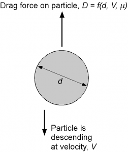
Check Your Understanding #2 – Drag on an aerosol particle
As shown in the figure below, a spherical aerosol particle of diameter (assumed in the sub-micron size range) falls freely vertically at velocity in air. Assume that the fluid’s viscosity is much more important than its density, so the effects of density (which manifests as buoyancy) can be ignored. Find the similarity parameter that governs the drag on the particle.
Show solution/hide solution.
Functional Dependence
The aerodynamic drag on the particle can be written in functional form as
![\[ D = \phi ( d, \, V, \, \mu ) \]](https://eaglepubs.erau.edu/app/uploads/quicklatex/quicklatex.com-ff88d54ded05cab081ee07f09b13e3f9_l3.svg "Rendered by QuickLaTeX.com")
where is the viscosity of the air and is some function to be determined. In implicit form, then
![\[ \psi (d, \, V, \, \mu, \, D ) = 0 \]](https://eaglepubs.erau.edu/app/uploads/quicklatex/quicklatex.com-eca9bb5d871fa5d101501221a15093be_l3.svg "Rendered by QuickLaTeX.com")
where is some other function. In this case,  and (by inspection, all of mass, length, and time are involved in this problem), so there are
  , i.e., one product.
Dimensional Matrix
Setting down the dimensional matrix, then
![\[ \begin{array}{l|r|r|r|r|r} \mbox{\small Base~unit} & d & V & \mu & D \\ \hline \text{\small Mass, M} \quad & 0 & 0 & 1 & 1 \\ \text{\small Length, L} \quad & 1 & 1 & -1 & 1 \\ \text{\small Time, T} \quad & 0 & -1 & -1 & -2 \end{array} \]](https://eaglepubs.erau.edu/app/uploads/quicklatex/quicklatex.com-19ffef385d82fe72509998362b8f857f_l3.svg "Rendered by QuickLaTeX.com")
Repeating Variables
The dependent variable ( in this case) cannot be a repeating variable, and so the only choice is , , and . This can also be confirmed by determining the determinant of the dimensional submatrix that is formed by the repeating variables, which shows that
![\[ \det \begin{bmatrix} 0 & 0 & 1 \\ 1 & 1 & -1 \\ 0 & -1 & -1 \end{bmatrix} \ne 0 \]](https://eaglepubs.erau.edu/app/uploads/quicklatex/quicklatex.com-45e24b2df2ddaecfb1d8b0345954196a_l3.svg "Rendered by QuickLaTeX.com")
Π product
For the only product, then
![\[ \Pi = (d)^{\alpha} (V)^{\beta} (\mu)^{\gamma} \, D \]](https://eaglepubs.erau.edu/app/uploads/quicklatex/quicklatex.com-948f22c6895715aab0cc2a5f7fb45a73_l3.svg "Rendered by QuickLaTeX.com")
and in terms of dimensions, then
![\[ \left[ \Pi \right] = \rm M^{0}L^{0}T^{0} =\rm (L)^{\alpha} \rm (L T^{-1})^{\beta} \rm (M L^{-1} T^{-1})^{\gamma} \rm M L T^{-2} \]](https://eaglepubs.erau.edu/app/uploads/quicklatex/quicklatex.com-dee35e5ca466be3357c8bc536f38ed18_l3.svg "Rendered by QuickLaTeX.com")
For the group to be dimensionless, then

Therefore, , and and so the product is
![\[ \Pi = (d)^{-1}(V)^{-1} (\mu)^{-1} D = \frac{D}{d V \mu} = C_D \]](https://eaglepubs.erau.edu/app/uploads/quicklatex/quicklatex.com-5264bfccf9de12c999ad6a6c9f3d0519_l3.svg "Rendered by QuickLaTeX.com")
which is a drag coefficient  applicable, in this case, to what is known as a Stokes flow.
Check
It is always good to check the final dimensions of the grouping to be sure it is dimensionless, i.e., it has dimensions of 1. So, in this case
![\[ \left[ C_D \right] = \frac{\rm M L T^{-2}}{(\rm L) (\rm L T^{-1}) (\rm M L^{-1} T^{-1})} = \frac{\rm M L T^{-2}}{\rm M L T^{-2}} = 1 \]](https://eaglepubs.erau.edu/app/uploads/quicklatex/quicklatex.com-7dcec091fb110bfbbdc43aaf3dd9239a_l3.svg "Rendered by QuickLaTeX.com")
which confirms that the grouping is dimensionless.
Check Your Understanding #3 – Equilibrium of a soap bubble
The equilibrium state of a soap bubble of diameter depends on a differential pressure balance,  , between its internal pressure relative to the ambient pressure as well as its surface tension,
  . Find the non-dimensional grouping that expresses this relationship. Hint: The base dimensions of surface tension is M L.
Show solution/hide solution.
Functional Dependency
The pressure difference can be written in functional form as
![\[ \Delta p = \phi (d, \, \sigma ) \]](https://eaglepubs.erau.edu/app/uploads/quicklatex/quicklatex.com-0714c9129ea2ef0df5b9bf70d26867d4_l3.svg "Rendered by QuickLaTeX.com")
or in implicit form as
![\[ \psi (d, \, \sigma, \, \Delta p )= 0 \]](https://eaglepubs.erau.edu/app/uploads/quicklatex/quicklatex.com-69dc246fea5905d739bcd694337699d6_l3.svg "Rendered by QuickLaTeX.com")
Therefore,  , , and there are no
  products! This is a special situation that can be resolved by reducing the number of repeating variables by one, i.e., setting = 2.
Dimensional Matrix
The dimensional matrix is
![\[ \begin{array}{l|r|r|r|r|r} \mbox{\small Base~unit} & d & \sigma & \Delta p \\ \hline \text{\small Mass, M} \quad & 0 & 1 & 1 \\ \text{\small Length, L} \quad & 1 & -2 & -1 \\ \text{\small Time, T} \quad & 0 & 0 & -2 \end{array} \]](https://eaglepubs.erau.edu/app/uploads/quicklatex/quicklatex.com-cf9c4ecc1c46dd9e304b84767d74a4a4_l3.svg "Rendered by QuickLaTeX.com")
Repeating Variables
The dependent variable ( in this case) cannot be a repeating variable, and so the only choice is and , which are linearly independent. This can also be confirmed by determining the determinant of the dimensional submatrix that is formed by the repeating variables, which shows that
(87) 
Derivation of the Π Product
The product is
![\[ \Pi = (d)^{\alpha} (\sigma)^{\beta} \Delta p \]](https://eaglepubs.erau.edu/app/uploads/quicklatex/quicklatex.com-d81b3273c687e1e5460596f5cc9326c5_l3.svg "Rendered by QuickLaTeX.com")
where the values of the coefficients and must be obtained to make the equation dimensionally homogeneous and dimensionless. In terms of the dimensions of the parameters, then
![\[ \left[ \Pi \right] = \rm M^{0}L^{0}T^{0} = \left( \rm L \right)^{\alpha} \left( \rm M T^{-2} \right)^{\beta} \left(\rm M L^{-1} T^{-2}\right) \]](https://eaglepubs.erau.edu/app/uploads/quicklatex/quicklatex.com-c06f334addb888a67cf031f73e12a512_l3.svg "Rendered by QuickLaTeX.com")
For to be dimensionless, then the powers or exponents of M, L, and T must add to zero, i.e., in this case

Therefore, , , so the product is
![\[ \Pi = \dfrac{\Delta p \, d}{\sigma} \]](https://eaglepubs.erau.edu/app/uploads/quicklatex/quicklatex.com-cd23545225ea0deda4229f6b38fb64d7_l3.svg "Rendered by QuickLaTeX.com")
Check
Check the final dimensions of the grouping to be sure it is dimensionless, i.e., it has dimensions of 1. So, in this case
![\[ \left[ \dfrac{\Delta p \, d}{\sigma} \right] = \dfrac{ (M L^{-1} T^{-2}) L }{M T^{-2} } = 1 \]](https://eaglepubs.erau.edu/app/uploads/quicklatex/quicklatex.com-cca48491d59bac80392aa5e2dc1efc00_l3.svg "Rendered by QuickLaTeX.com")
Check Your Understanding #4 – Orbital decay of a satellite in low Earth orbit
The orbital decay of a satellite in low earth orbit (LEO), given by  (=
(=  ), is known to be a function of the orbital radius,
  , the density of the air, , in the upper atmosphere, the size of the satellite in terms of a reference area,
  , the aerodynamic drag on the satellite,
  , the mass of the satellite,
  , and acceleration under gravity, . Find the dimensionless groupings that will govern this problem.
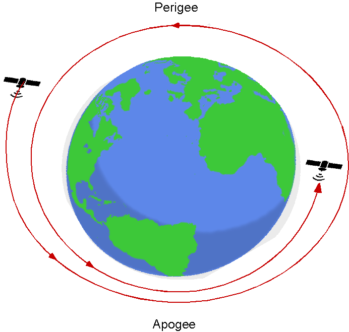
Show solution/hide solution.
Functional Dependency
By using the information provided then, the orbital decay in LEO can be written in an explicit functional form as
(88) 
where  is some function, or the information can be written in implicit form as
![\[ \psi_2 \left( \overbigdot{R_s} , \varrho, \, A_{\rm ref}, \, D, \, m_s, \, g, \, R_s, \, V_s \right) = 0 \]](https://eaglepubs.erau.edu/app/uploads/quicklatex/quicklatex.com-3ba7d9eb8239d66c58d814b3f23c0b27_l3.svg "Rendered by QuickLaTeX.com")
where  is some other function. Therefore,
  , , and so there are five products to find in this case. This is a little more complex problem in dimensional analysis, but the principles are the same.
Dimensional Matrix
Forming the dimensional matrix from the base dimension of each of the parameters gives
![\[ \begin{array}{l|r|r|r|r|r|r|r|r} \mbox{\small Base~unit} & \overbigdot{R_s} & \varrho & A_{\rm ref} & D & m_s & g & R_s & V_s \\ \hline \text{\small Mass, M} & 0 & 1 & 0 & 1 & 1 & 0 & 0 & 0 \\ \text{\small Length, L} & 1 & -3 & 2 & 1 & 0 & 1 & 1 & 1 \\ \text{\small Time, T} & -1 & 0 & 0 & -2 & 0 & -2 & 0 & -1 \end{array} \]](https://eaglepubs.erau.edu/app/uploads/quicklatex/quicklatex.com-cf46ece73581eb21fc7ce9ad9a24105a_l3.svg "Rendered by QuickLaTeX.com")
Repeating Variables
The repeating variables must collectively include the dimensions of mass  , length
  , and time
  , so one choice here is ,
  , and
, and  , all of which have a primary dependence on the orbital decay and by inspeaction they are also linearly independent. Alternatively, , , and could be used. But if were to be chosen instead of
  as a repeating variable, then collectively, the repeating variables would not include mass, ; the Buckingham method will fail in this case. Notice also that it would not be appropriate to use the satellite’s mass, , as a repeating variable because the orbital characteristics, such as velocity and period, are independent of the mass. The dependent variable, , cannot be used as a repeating variable.
This can also be confirmed by determining the determinant of the dimensional submatrix that is formed by the repeating variables, which shows that
(89) 
Π Products
Therefore, the five products are formed from
![\[ \Pi_1 = \phi_1(\varrho, R_s, V_s, \overbigdot{R_s} ) \]](https://eaglepubs.erau.edu/app/uploads/quicklatex/quicklatex.com-23e745bc99c7b04804cf9d323a62d24a_l3.svg "Rendered by QuickLaTeX.com")
![\[ \Pi_2 = \phi_2(\varrho, R_s, V_s, D ) \]](https://eaglepubs.erau.edu/app/uploads/quicklatex/quicklatex.com-2c65c09f15f0dcc6d9a5e52e27afbfd8_l3.svg "Rendered by QuickLaTeX.com")
![\[ \Pi_3 = \phi_2(\varrho, R_s, V_s, m_s ) \]](https://eaglepubs.erau.edu/app/uploads/quicklatex/quicklatex.com-0599d180118956ad6a44b52b1c3c7ce5_l3.svg "Rendered by QuickLaTeX.com")
![\[ \Pi_4 = \phi_2(\varrho, R_s, V_s, g ) \]](https://eaglepubs.erau.edu/app/uploads/quicklatex/quicklatex.com-b4bf5ae03faa355e10dffacd30eedc28_l3.svg "Rendered by QuickLaTeX.com")
![\[ \Pi_5 = \phi_2(\varrho, R_s, V_s, A_{\rm ref} ) \]](https://eaglepubs.erau.edu/app/uploads/quicklatex/quicklatex.com-582b19dc7c334bd12d085dc1afbaa999_l3.svg "Rendered by QuickLaTeX.com")
Derivation of the Π Products
The first product is formed from
![\[ \Pi_{1} = (\varrho)^{\alpha} (R_s)^{\beta} (V_s)^{\gamma} \, \overbigdot{R_s} \]](https://eaglepubs.erau.edu/app/uploads/quicklatex/quicklatex.com-3cd8460346ba822ab6c5bfaa276369bc_l3.svg "Rendered by QuickLaTeX.com")
where the values of the coefficients , , and must be obtained to make the equation dimensionally homogeneous and dimensionless. In terms of the dimensions of the parameters, then
![\[ \left[ \Pi_{1} \right] = \rm M^{0}L^{0}T^{0} = \left( \rm M L^{-3} \right)^{\alpha} \left( \rm L \right)^{\beta} \left( \rm L T^{-1} \right)^{\gamma} \left(\rm L T^{-1}\right) \]](https://eaglepubs.erau.edu/app/uploads/quicklatex/quicklatex.com-8bfb607e6cf6ff4b0c3c17df08c3b833_l3.svg "Rendered by QuickLaTeX.com")
For to be dimensionless, then the powers or exponents of M, L, and T must add to zero, i.e.,

Therefore, in this case , , and  , so the
  product is
![\[ \Pi_1 = (\varrho)^{0} (R_s)^{0} (V_s)^{-1} \, \overbigdot{R_s} = \dfrac{\overbigdot{R_s}}{V_s} \]](https://eaglepubs.erau.edu/app/uploads/quicklatex/quicklatex.com-82af5caf5498f384420fbfdec04f42d9_l3.svg "Rendered by QuickLaTeX.com")
which is a dimensionless decay rate that is a fraction of the orbital velocity.
The second product involves the drag force, , i.e.,
![\[ \Pi_2 = (\varrho)^{\alpha} (R_s)^{\beta} (V_s)^{\gamma} \, D \]](https://eaglepubs.erau.edu/app/uploads/quicklatex/quicklatex.com-cec88dbead8a531489fb3fa4633a891a_l3.svg "Rendered by QuickLaTeX.com")
In terms of the dimensions, then
![\[ \left[ \Pi_2 \right] = \rm M^{0}L^{0}T^{0} = \left( \rm M L^{-3} \right)^{\alpha} \left( \rm L \right)^{\beta} \left( \rm L T^{-1} \right)^{\gamma} \left(\rm M L T^{-2}\right) \]](https://eaglepubs.erau.edu/app/uploads/quicklatex/quicklatex.com-f2ebed9fd4127f0937539ea0fac6ca66_l3.svg "Rendered by QuickLaTeX.com")
For to be dimensionless, then

Solving these equations gives , , and , so the product is
![\[ \Pi_2 = (\varrho)^{-1} (R_s)^{2} (V_s)^{-2} \, D = \frac{D}{\varrho \, R_s^2 \, V_s^2} \]](https://eaglepubs.erau.edu/app/uploads/quicklatex/quicklatex.com-5f76e21b006fa863e64a586699bc98ae_l3.svg "Rendered by QuickLaTeX.com")
which is a form of drag coefficient. It is legitimate to replace  by and multiply the denominator by 1/2 to obtain the conventional form of drag coefficient, i.e.,
![\[ \Pi_2 = \dfrac{D}{\dfrac{1}{2} \varrho \, A_{\rm ref} \, V_s^2} \]](https://eaglepubs.erau.edu/app/uploads/quicklatex/quicklatex.com-008db487829a248f8b99b4a49bf0176e_l3.svg "Rendered by QuickLaTeX.com")
The third product involves the satellite mass, , i.e.,
![\[ \Pi_3 = (\varrho)^{\alpha} (R_s)^{\beta} (V_s)^{\gamma} \, m_s \]](https://eaglepubs.erau.edu/app/uploads/quicklatex/quicklatex.com-1af5a3aa56aa0c2f2188f138f0f3ae45_l3.svg "Rendered by QuickLaTeX.com")
In terms of the dimensions, then
![\[ \left[ \Pi_3 \right] = \rm M^{0}L^{0}T^{0} = \left( \rm M L^{-3} \right)^{\alpha} \left( \rm L \right)^{\beta} \left( \rm L T^{-1} \right)^{\gamma} \, \rm M \]](https://eaglepubs.erau.edu/app/uploads/quicklatex/quicklatex.com-a3ce35249aae824716b5060bb30df675_l3.svg "Rendered by QuickLaTeX.com")
For  to be dimensionless, then

Solving these, gives , , and  , so the product is
![\[ \Pi_3 = (\varrho)^{-1} (R_s)^{-3} (V_s)^{0} \, m_s = \frac{m_s}{\varrho \, R_s^3} \]](https://eaglepubs.erau.edu/app/uploads/quicklatex/quicklatex.com-676ad31cedd498f5d93c95165d7ca141_l3.svg "Rendered by QuickLaTeX.com")
or inverting the grouping because a low value will make the parameter large, then
![\[ \Pi_3 = \frac{\varrho \, R_s^3}{m_s} \]](https://eaglepubs.erau.edu/app/uploads/quicklatex/quicklatex.com-a37e8dd29b47ce36113b2003a9a0c7a0_l3.svg "Rendered by QuickLaTeX.com")
which is a form of buoyancy ratio. The value of this parameter in space is likely to be so small, even in a low Earth orbit, that it can be justifiably neglected.
The fourth product involves the gravitational acceleration, , i.e.,
![\[ \Pi_4 = (\varrho)^{\alpha} (R_s)^{\beta} (V_s)^{\gamma} \, g \]](https://eaglepubs.erau.edu/app/uploads/quicklatex/quicklatex.com-60f9517330fadfa510be797ac56c2f1a_l3.svg "Rendered by QuickLaTeX.com")
In terms of the dimensions, then
![\[ \left[ \Pi_4 \right] = \rm M^{0}L^{0}T^{0} = \left( \rm M L^{-3} \right)^{\alpha} \left( \rm L \right)^{\beta} \left( \rm L T^{-1} \right)^{\gamma} \left(\rm L T^{-2}\right) \]](https://eaglepubs.erau.edu/app/uploads/quicklatex/quicklatex.com-eba2f6595dbdda4e2495f7c4b6bdca0e_l3.svg "Rendered by QuickLaTeX.com")
For  to be dimensionless, then

Solving these, gives , , and , so the product is
![\[ \Pi_4 = (\varrho)^{0} (R_s)^{1} (V_s)^{-2} \, g = \frac{g \, R_s}{V_s^2} \]](https://eaglepubs.erau.edu/app/uploads/quicklatex/quicklatex.com-aa81051f8afebcba8ebfc8f2f9a5fbfc_l3.svg "Rendered by QuickLaTeX.com")
which is a ratio of potential energy to kinetic energy. This outcome will be apparent by multiply the numerator and the denominator by the satellite’s mass.
The fifth product involves the reference area, , i.e.,
![\[ \Pi_5 = (\varrho)^{\alpha} (R_s)^{\beta} (V_s)^{\gamma} \, A_{\rm ref} \]](https://eaglepubs.erau.edu/app/uploads/quicklatex/quicklatex.com-27c45b8b5d1478874f5ff51d32f9c9b3_l3.svg "Rendered by QuickLaTeX.com")
In terms of the dimensions, then
![\[ \left[ \Pi_5 \right] = \rm M^{0}L^{0}T^{0} = \left( \rm M L^{-3} \right)^{\alpha} \left( \rm L \right)^{\beta} \left( \rm L T^{-1} \right)^{\gamma} \left(\rm L^2\right) \]](https://eaglepubs.erau.edu/app/uploads/quicklatex/quicklatex.com-1bb82ac8848abba64a62a43f6181a428_l3.svg "Rendered by QuickLaTeX.com")
For  to be dimensionless, then

Solving these equations, gives , , and . Therefore, the product is
![\[ \Pi_5 = (\varrho)^{0} (R_s)^{-2} (V_s)^{0} \, A_{\rm ref} = \frac{A_{\rm ref}}{R_s^2} \]](https://eaglepubs.erau.edu/app/uploads/quicklatex/quicklatex.com-4c4407a3cb26ad93fc1d72f1193d939f_l3.svg "Rendered by QuickLaTeX.com")
which is an area ratio, although of little significance in this problem.
Final Dimensionless Form
In summary, the five products are:
![\[ \Pi_1 = \frac{\overbigdot{R_s}}{V_s}, \quad \Pi_2 = \frac{D}{\dfrac{1}{2}\varrho \, A_{\rm ref} \, V_s^2}, \quad \Pi_3 = \frac{\varrho \, R_s^3}{m_s}, \quad \Pi_4 = \frac{g \, R_s}{V_s^2}, \quad \Pi_5 = \frac{A_{\rm ref}}{R_s^2} \]](https://eaglepubs.erau.edu/app/uploads/quicklatex/quicklatex.com-3302f752a39020d57ee5d46420baa81a_l3.svg "Rendered by QuickLaTeX.com")
The final relationship can be written as a function of these dimensionless groups as
![\[ \phi_1\left( \frac{\overbigdot{R_s}}{V_s}, \ \dfrac{D}{\dfrac{1}{2}\varrho \, A_{\rm ref} V_s^2}, \ \frac{\varrho \, R_s^3}{m_s}, \ \frac{g \, R_s}{V_s^2}, \ \frac{A_{\rm ref}}{R_s^2} \right) = 0 \]](https://eaglepubs.erau.edu/app/uploads/quicklatex/quicklatex.com-9d9a86415c238630fa73cbfe587011e6_l3.svg "Rendered by QuickLaTeX.com")
Removing the irrelevant or redundant terms in writing in explicit form gives
![\[ \frac{\overbigdot{R_s}}{V_s} = \psi_2 \left( \dfrac{D}{\dfrac{1}{2}\varrho \, A_{\rm ref} \, V_s^2}, \ \frac{g R_s}{V_s^2} \right) \]](https://eaglepubs.erau.edu/app/uploads/quicklatex/quicklatex.com-38bffd0829af2f83853fe982064ea836_l3.svg "Rendered by QuickLaTeX.com")
Therefore, a satellite’s dimensionless radial decay in LEO is a function of its aerodynamic drag coefficient ( is often assumed) and the ratio of the potential to kinetic energy (usually about 1).
Other Dimensionless Quantities
In engineering practice, it is common to work with dimensionless quantities or to normalize dimensional quantities by appropriate reference values to make them dimensionless. This approach simplifies mathematical expressions and allows the use of standard mathematical functions without introducing units.
Some physical variables are naturally dimensionless by their definition, i.e., as ratios of the same dimensional quantities. One example often encountered in thermodynamics and aerodynamics is the ratio of specific heats,  . Another example of a naturally dimensionless parameter used in structural analysis is strain, which is defined as the ratio of the change in length of a structural component under loading, , compared to its initial length, , i.e., the strain is
  . Finally, in hydrostatics, the specific gravity,
  , which is a dimensionless number defined as the ratio of the density of a given liquid relative to the density of water, is often used.
It should be remembered that all angles are dimensionless. In engineering analysis, angles measured in radians are always used, defined as a ratio of the arc length to the radius of a circle. The dimensions of a radian are 1, i.e., it is unitless. While angles are often measured or reported in degrees, units of degrees must be converted to radians for most engineering calculations. A complete circle subtends an angle of  radians. which is equivalent to 360 degrees or 360, so the angular conversion is 1 radian =
  degrees. The same should also be done with angular rates, which should always be converted to radians per second (rad/s) no matter what units the rates are originally given in, e.g., rates are often measured in revolutions per minute (rpm) or revolutions per second (rps). The dimensions of angular rate are T as is revolutions per unit time.
When dealing with trigonometric and exponential functions, the arguments must be dimensionless; using them with dimensional values is incorrect. Consider the following examples:
- In trigonometry, angles are measured in radians, which is a dimensionless angle. Therefore, all trigonometric expressions such as
 and
and  are valid only when and are in units of radians. For example, if has units of length (typical in engineering), then the equation
  is invalid. However, if the lengths are non-dimensionalized by a fixed reference length such as , then
  is a valid equation.
 - The exponential function
 , which occurs frequently in engineering, is also defined for dimensionless arguments. If the variable
  has units of time, then the equation
  is invalid. However, if
  is a frequency (units of radians per second), then
  is a valid equation. Likewise, if is a reference time (units of seconds), then
  is a valid equation.
When Things Go Wrong in the Buckingham Π Method
The Buckingham method is a powerful tool for constructing dimensionless groupings, but certain issues can arise that cause the method to fail or otherwise provide meaningful results. Common problems with more complex problems with more dependencies and fundamental dimensions include the inability to find a set of linearly independent repeating variables, failing to include all fundamental dimensions, or ending up with an underdetermined system that does not yield a unique set of dimensionless groups.
- No Linearly Independent Set of Repeating Variables:
This issue occurs when a dimensionless variable (such as the ratio of specific heats
) is chosen as a repeating variable, or the selected repeating variables can form a dimensionless group among themselves. In either case, the dimensional vectors will be linearly dependent, i.e., the resulting matrix does not have full rank. Therefore, repeating variables must be dimensionally independent and span all fundamental dimensions used in the problem. For example, consider the variables:(90)
![\begin{equation*} \begin{array}{rl} \gamma: & \text{dimensionless} \\ V: & \text{velocity}, \ [V] = \rm L T^{-1} \\ c: & \text{length}, \ [c] = \rm L \\ \mu: & \text{dynamic viscosity}, \ [\mu] = \rm M L^{-1} T^{-1} \end{array} \end{equation*}](https://eaglepubs.erau.edu/app/uploads/quicklatex/quicklatex.com-5f92ec32d3b1165a3ca7123a22834cdd_l3.svg "Rendered by QuickLaTeX.com")
If
, , and are chosen as repeating variables, the resulting dimensional sub-matrix is(91)

Therefore,
(92)

which makes the set linearly dependent. A valid set of repeating variables must be linearly independent and span all fundamental dimensions in the problem. Therefore, this choice is invalid.
![\[\]](https://eaglepubs.erau.edu/app/uploads/quicklatex/quicklatex.com-4aabddc1c342c8ef16735dbd83bd3e5b_l3.svg "Rendered by QuickLaTeX.com")
- Not All Fundamental Dimensions Are Represented:
Even with linearly independent repeating variables, the selection is invalid if it does not cover all fundamental dimensions, e.g., M, L, T. The rule is that the repeating variables must span the entire dimensional space of the problem. Consider the following variables:
(93)
![\begin{equation*} \begin{array}{rl} V: & \text{velocity},\ [V] = \rm L T^{-1} \\ c: & \text{length},\ [c] = \rm L \\ g: & \text{gravitational acceleration},\ [g] = \rm L T^{-2} \\ \varrho: & \text{density},\ [\varrho] = \rm M L^{-3} \end{array} \end{equation*}](https://eaglepubs.erau.edu/app/uploads/quicklatex/quicklatex.com-d825ae784573deca5cbb8eb5d286a758_l3.svg "Rendered by QuickLaTeX.com")
Suppose the chosen repeating variables are
 , , and
  . Their dimensional representations are
(94)

Therefore,
(95)

The determinant is zero because all rows have a zero for the mass dimension, so the matrix lies entirely within the L-T subspace. Although the vectors are linearly independent within that subspace, they do not include all of M, L, and T. Therefore, it is not possible to non-dimensionally combine a variable such as
, which includes the mass dimension, using only the selected repeating variables. Therefore, this is an invalid selection of repeating variables, even though the vectors are linearly independent. - Indeterminate Solutions and Non-Unique Groups:
Sometimes, the system of equations has infinitely many solutions, meaning the resulting
groups are not unique. This happens when too many repeating variables are chosen, or the selection is not well-posed. As an example where the repeating variables form a dimensionless, consider the variables:(96)

Suppose the repeating variables are chosen as
, , and . The determinant of their dimensional vectors is(97)

which is zero, showing that the chosen variables are linearly dependent. This means that
, , and cannot be used together as repeating variables. These variables can also form a dimensionless group(98)

This confirms that they are not dimensionally independent. A useful warning sign is that the variables all share similar or overlapping dimensions, and none include all base units.
- Indeterminate System From Too Many Repeating Variables:
Consider a problem involving the following five variables, all expressed in terms of only two fundamental dimensions, L and T, i.e.,
(99)

This system involves only two base dimensions, L and T. The number of independent dimensionless groups should be
= 5 – 2 = 3. Suppose the repeating variables are chosen as , , and . Their dimensional representations are(100)

This set includes three vectors, but only two fundamental dimensions are involved. As a result, the system of equations used to construct the
groups is underdetermined: there are more unknowns (the power or exponents) than there are equations (base dimensions).This leads to infinite valid solutions and non-unique
groups. The method no longer produces a unique or minimal set of dimensionless parameters. To resolve this, the number of repeating variables must be reduced to exactly two, i.e., matching the number of base dimensions. For example, selecting and as repeating variables yields a valid, well-posed system that produces three unique groups involving the remaining variables , , and  .
. - Using repeating variables that could form their own dimensionless group:
Repeating variables must not form a dimensionless group among themselves. For example, it would be inappropriate to choose
, , and one other variable (e.g., or ) as repeating variables in dimensional analysis. While these variables are dimensionally independent in a strict algebraic sense, they can combine to form a dimensionless group, specifically, the Reynolds number  . This violates a critical requirement of the Buckingham Pi theorem, i.e., the repeating variables must not form a dimensionless product among themselves. Doing so introduces redundancy, undermines dimensional independence, and can produce spurious or non-unique dimensionless groups.
As a reminder, the four main rules as to how to choose the repeating variables are:
- Do not choose the dependent variable as a repeating variable.
- Choose repeating variables likely to have the most important effects on the dependent variable.
- The repeating variables must collectively include all of the base dimensions.
- The repeating variables must be linearly independent. In general, do not choose repeating variables with the same base dimensions or base dimensions that differ by an exponent.
Remember that the determinant of the submatrix formed by the dimensions of the selected repeating variables should not equal zero. If it is zero, then the method will fail.
In practice, this also means that:
- Do not use dimensionless variables as repeating variables.
- Avoid using repeating variables that are likely to form their own dimensionless group.
Again, in both of these latter cases, if the determinant of the submatrix formed by the dimensions of the selected repeating variables is zero, then this selection will cause the method to fail.
Finally, if the system is underdetermined, i.e., too many dimensions and not enough repeating variables that meet the four rules, then the recommended approach is to reduce the number of repeating variables by one, and then form one additional group.
Summary & Closure
Dimensional analysis can be a powerful tool for engineering analysis because it reduces and simplifies the size and scope of the problem in terms of dimensionless or non-dimensional groupings called similarity parameters. The strength of dimensional analysis as a tool usually becomes apparent when applied to increasingly more complicated engineering problems, such as where the effects of all the dependencies cannot be established explicitly and/or the governing equations for the solution of the problem can become formidably complicated. For example, it is common for engineering problems to have five, six, seven, or even more dependencies. However, sorting out the problem parameters into dimensionless groupings helps to understand what parameters are essential as they will affect the physical behavior and what parameters are not.
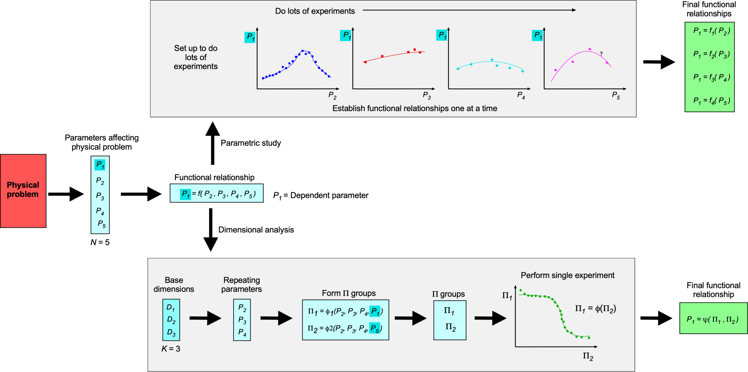 method. (Click on the image for a bigger version.)
Dimensional analysis must be used in a systematic and structured approach, formally embodied in the Buckingham method. A critical first step is to carefully lay out the problem in terms of the dependent and independent quantities, which must all be assigned the correct base dimension. While the choice of the repeating quantities is somewhat arbitrary, specific rules must be followed for the method to work. For example, it is critical that the dependent quantity is not used as a repeating variable. The repeating variables must also have substantial effects on the dependent quantity and be linearly independent of each other, i.e., two repeating parameters with the same dimensions cannot be used, such as two reference length scales or two reference velocities. If the basic rules of the Buckingham method are followed, then the outcomes will be groups of dimensionless parameters that should not only help understand the problem but will simplify its scope.
5-Question Self-Assessment Quickquiz
For Further Thought or Discussion
- You are tasked with explaining to a high-school student studying physics the advantages of using dimensional analysis and dimensionless quantities. What two primary arguments would you make?
- The force on a body in the wind tunnel is known to depend on flow velocity (airspeed) and the static pressure and temperature in the flow. What other parameters may be involved? Hint: Do not suggest parameters such as viscosity or the speed of sound.
- Use dimensional analysis to show that the drag of a ship’s hull, in part, depends on the Froude number. The Froude number is defined as
 , where is the length of the ship and is the speed of the ship through the water.
 - You are tasked with determining the hydrodynamic drag force on a fully submerged, very long, neutrally buoyant cable dragged behind a ship. You propose to do this by doing small-scale experiments in a water tunnel. Determine the dimensionless groupings that will affect this problem.
- Show that the pressure drop caused by a restrictor in a flow can be expressed in terms of the Euler number
 , where the pressure drop is expressed in terms of an energy loss in the flow per unit of kinetic energy per volume of the flow.
Other Useful Online Resources
To dive deeper into the methods of dimensional analysis, navigate to the following online resources:
- Description of dimensional analysis on Wikipedia.
- YouTube video on the Buckingham method.
- YouTube Video of an example of using the Buckingham method.
