Introduction

Aerospace engineering students soon begin to ask when they can start to solve actual problems relevant to aircraft, rockets, or spacecraft. Of course, it is natural to ask such questions, even in the early stages of an engineering education. However, practical problem-solving in engineering is a serious business that requires engineers-in-training to become well-versed in the fundamental subjects relevant to their field. In addition to the usual engineering disciplines, this process of learning and becoming proficient will inevitably require a solid foundation in physics, chemistry, mathematics, numerical methods, and computer programming.

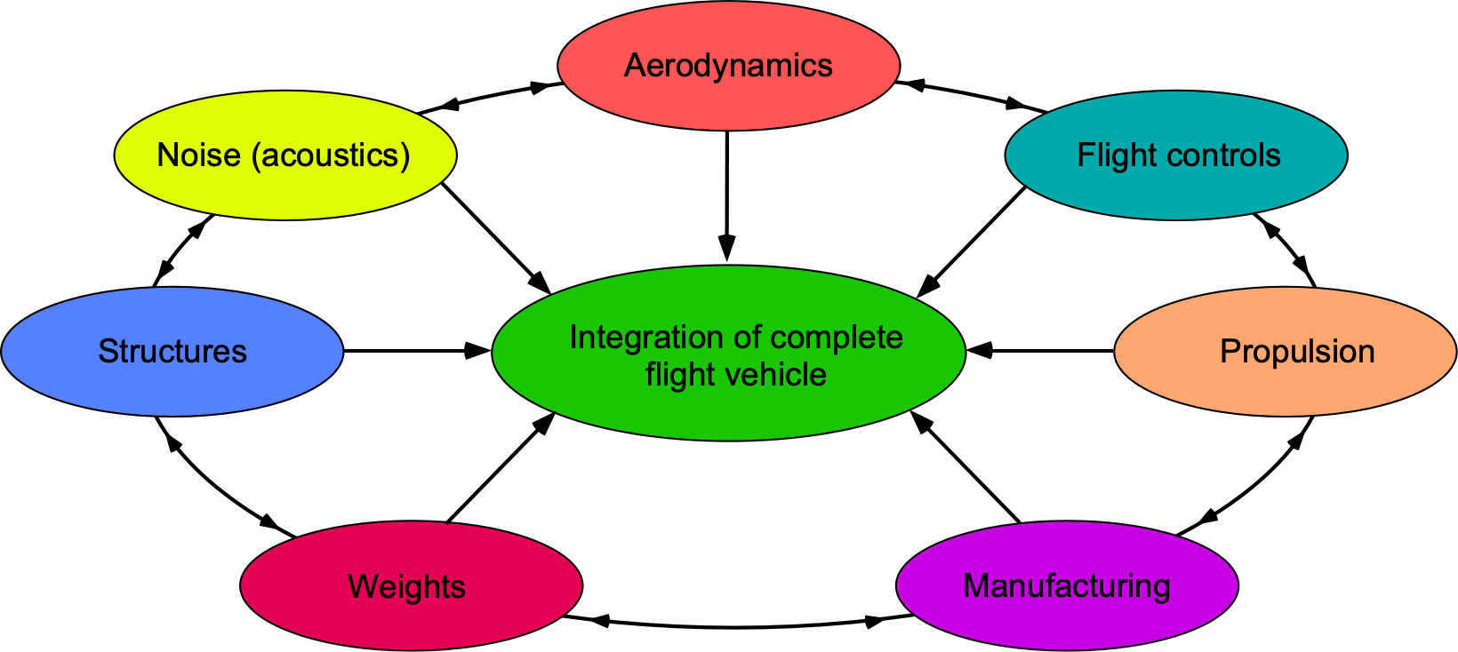
In general, engineering problem-solving is an established and well-proven process in which the bigger problem is first dissected into smaller, more manageable, and perhaps better digestible parts, as illustrated in the figure below for a flight vehicle. However, the smaller parts are not mutually exclusive. Then, each vehicle component can be analyzed separately, at least initially, perhaps through experiments, mathematical models, numerical models, or a combination of these working approaches. Finally, the understanding and functionality of the parts can be reassembled using a synthesis approach to comprehend the flight vehicle as a whole, considering interactions as well. Of course, such an approach is always flawed, but it forms at least one rational basis for understanding and designing complex engineering systems, including aircraft and spacecraft.

Today, aerospace engineers must also have increasingly multidisciplinary technical skill sets, which means they must follow a broader-based educational path and become more knowledgeable and versatile in using a more comprehensive range of subject matter. It is no longer sufficient to be an aerodynamics specialist or “aerodynamicist,” or a “structural dynamicist,” or an “acoustician.” Successful aerospace engineers must be technically broad and increasingly versatile to work with others in interdisciplinary contexts.

Furthermore, artificial intelligence (AI), machine learning, and big data analytics are becoming increasingly prevalent in the aerospace industry, and engineers must understand the benefits and limitations of these technologies. As the industry evolves and tackles increasingly complex problems, it is also crucial that aerospace engineers continually develop their problem-solving skills throughout their careers to stay current with the latest technological advancements.

Hypothetico-Deductive Method

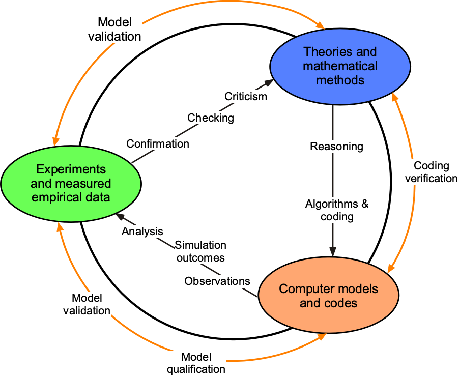
Many have argued that the engineering design process must follow the hypothetico-deductive method (or H-D method), a primary method for testing hypotheses or conjectures. The “hypothetico” (or hypothetical) part involves proposing a hypothesis or theory that needs to be tested, and the “deductive” part involves drawing conclusions from the hypothesis or hypotheses.^[1] The H-D method is sometimes called THE scientific method, but it is not the only method used in scientific and engineering work. The H-D method can be divided into four stages, as outlined in the figure below.

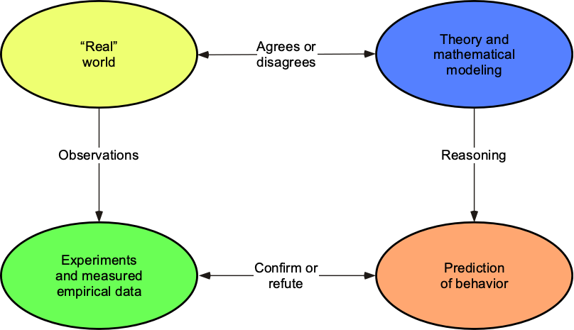
1. Identify the theory, the hypothesis, or the conjecture to be tested. This approach does not necessarily need to rely on facts and allows for “imaginative preconceptions, intuition, and even luck.” However, the hypothesis usually relies on prior understanding or awareness of pervasive laws.

2. Generate predictions from the theory. Theories are used to make predictions about what we see, i.e., we proceed to imitate what we perceive as the “real world.” These predictions would also encompass the range of conditions perceived as the theory’s domain of applicability, which cannot necessarily have limitless bounds and will trade off cost with theoretical complexity and value with predictive fidelity.

3. Use various types of experiments and measurements to test whether predictions are, in fact, correct. If done correctly, the measurements represent the truth. The data acquired, assuming the necessary quantities can be measured to the required levels of fidelity, provide the evidence to test the proposed theories. Replicating an experiment by others and repeating the data over time are critical to doing good science. The data may often uncover unexpected outcomes and spawn new directions if it is sufficiently comprehensive and of high quality.

4. Expose the theory to criticism, then reject or modify the theory or declare that the theory has been validated or otherwise proved. This process may take a significant amount of time and often depends on specific experimental measurements and the availability of other relevant data. However, it is the most crucial part of doing scientific research. Alternative hypotheses may be pursued after criticism to see which is more likely to explain the predictions. In this regard, the principle of parsimony, or Ockham’s Razor, is essential in mathematical modeling, i.e., in generating equations and mathematical models to represent any given physical behavior.

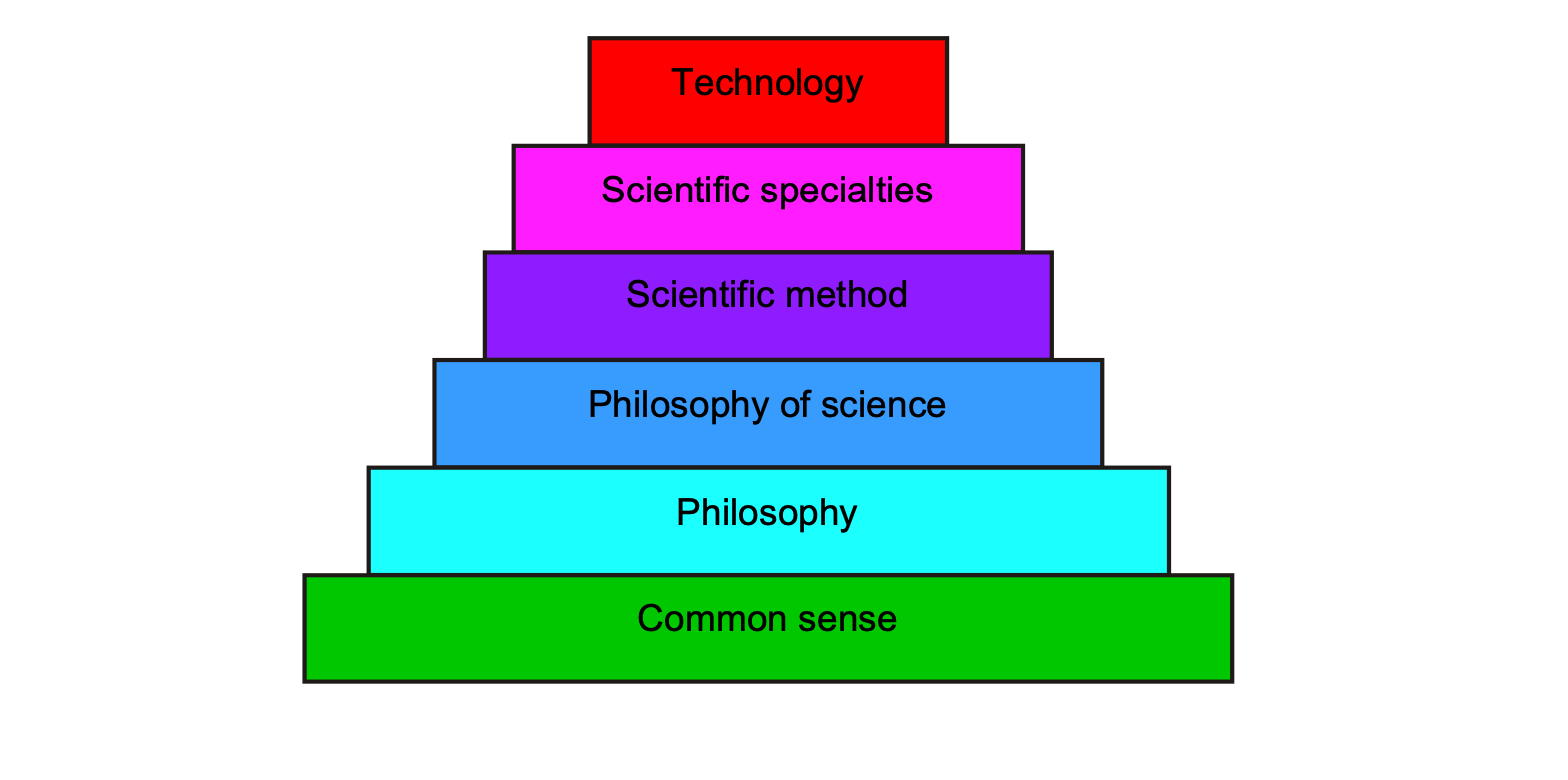
The overarching goal is to maintain a balance between modeling complexity and predictive fidelity. This can be achieved through careful, systematic validation studies and requires a degree of engineering common sense. After all, as the figure below suggests, this is the ultimate foundation on which the scientific method is based.

Other methods are used in scientific and engineering work. For example, descriptive methods observe and describe phenomena, while experimental methods manipulate variables to establish causal relationships. Correlational studies examine the relationships between variables without manipulation. Qualitative research gathers in-depth insights through non-numerical data, while mixed-methods research combines quantitative and qualitative approaches. Longitudinal studies track changes over time, meta-analysis synthesizes findings from multiple studies, and action research collaborates to address practical issues. Each method offers unique strengths suited to different research questions and objectives, guiding scientific exploration across diverse disciplines and contexts. Nevertheless, the hypothetico-deductive method remains the primary method for testing scientific and engineering hypotheses.

Starting Out

As students delve deeper into engineering concepts and various types of problem-solving in aerodynamics, structures, flight vehicle performance, and other areas, some cautionary words are warranted. First, it is essential to appreciate that there are few “handy equations” for solving engineering problems, especially in aerodynamics. Instead, the relevant equations for problem-solving must be selected carefully, based on the specific equations that most accurately govern the problem, known as the governing equations.

Choosing the governing equations is one issue, but solving them using the correct boundary conditions, and perhaps with any appropriate simplifications, involves considerable skill that comes only from much practice, i.e., consistent, purposeful, and focused practice over time. The solutions to some of these problems become homework exemplars of the field. “Those who study a scientific discipline are expected to know its exemplars.” Exemplars are “Key examples chosen so as to be typical of designated levels of quality of competence.”^[2] There is no fixed set of exemplars in aerospace engineering; however, this e-book is filled with a few hundred to start. Quo plus facit, eo magis peritus fit.

Aerodynamics

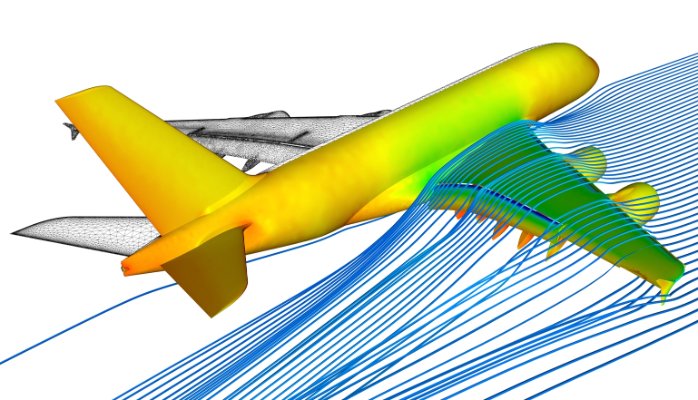
Remember that aerodynamics is the underpinning of flight; therefore, some form of aerodynamic analysis, as shown in the figure below, applies to almost all types of problem-solving involving aircraft and even spacecraft, including launch and re-entry vehicles. Therefore, it is essential that the selected aerodynamic models be sufficiently comprehensive and detailed to predict what is needed and for the right reason. Ultimately, they will provide a more substantial basis for informed decision-making, effective resource allocation, prudent risk management, and enhanced adaptability. By considering a wide range of factors and understanding the underlying reasons, it becomes possible to navigate options and reduce uncertainties, making informed choices.

Value-Based Analysis

The level of detail and comprehensiveness required in any mathematical model will depend on the specific type and complexity of the physical problem, which also affects the time and effort (i.e., cost) required to solve it. If the model is intended for precise predictions, design optimization, or critical engineering applications, a higher level of detail and accuracy is typically required, and the penalty is time for a solution. In the workplace, time is equivalent to money; therefore, a value-based decision process is necessary, making it essential to balance the technical level of detail in the model with the resulting computational cost.

Mathematical models must consider additional factors such as non-linearities, coupling effects, boundary interactions, or time-dependent behavior. These complexities require more comprehensive models that incorporate greater detail to accurately represent the physical problem and its behavior, albeit at the expense of longer execution times and higher costs. For example, aerodynamic equations may need to be solved consistently and simultaneously with other sets of equations that describe the behavior of different aspects of the aircraft, such as its dynamic flight motion, aeroelasticity, and acoustics.

It is soon concluded that problem-solving in engineering, especially concerning flight vehicles, can be very challenging, time-consuming, and costly because the mathematical forms of the governing equations for different disciplines will inevitably differ. This issue requires different solution methods, including various specific techniques, numerical methods, and others, which may be required in each case. For example, this may involve numerically solving the governing equations together or coupling them, as applicable, in different engineering fields.

Governing Equations

As students learn more about aerospace engineering disciplines, they will be exposed to more general forms of potentially applicable governing equations in each field. In many cases, the relevant governing equations that apply to a given problem may be subsets of more general governing equations intended to apply to a broader range of issues and conditions. In other cases, the governing equations may need to be developed from first principles, for example, by directly invoking the conservation principles of mechanics and thermodynamics. However, the approach must be systematic when choosing or creating the equations that apply to or govern a specific problem. The approach of picking a few equations and hoping they will apply is called an ad hoc approach. However, such an approach will inevitably prove disastrous; engineering case histories and experience speak for themselves.

Problem-solving also requires understanding the meaning of the governing equations, as well as each of the terms that comprise these equations. There may be terms or groups of terms in these equations that have different levels of complexity and may also have interdependencies, so dropping one term may have unintended consequences on the evaluation of other terms. In many cases, simplified (reduced) or otherwise particular governing equations may be appropriate because they simplify the solution process. Indeed, an approximate (and fast) solution might be adequate in the initial design phases. However, a more accurate (and likely more time-consuming) solution might be needed later. Part of the skill that must be developed in engineering problem-solving is determining which terms in the equations can be retained and which can be eliminated without substantially affecting the final solution’s outcomes.

Setting Up Aerodynamic Models

Solving problems in aerodynamics requires setting up the appropriate and applicable mathematical models of the flow correctly. The derivation of the mathematical equations that describe fluid dynamics and aerodynamic flows is a systematic process that has become well-established in engineering practice. However, because air (like all fluids) will continuously deform as it flows, its behavior must naturally be expected to be more difficult to describe than that of a solid material.

The starting point of any aerodynamic analysis is the statement of the physical problem, a definition of the appropriate boundary conditions, and making justifiable assumptions and approximations about how the flow develops. An example of a boundary condition defines the values of the freestream flow conditions or how the flow behaves on a boundary or surface, such as when it flows parallel to the surface. The three fundamental conservation principles of mechanics must then be applied to the aerodynamic problem, namely:

1. Conservation of mass, i.e., mass is neither created nor destroyed.
2. Conservation of momentum, i.e., a force applied to a mass equals its time rate of change of momentum.
3. Conservation of energy, i.e., energy is neither created nor destroyed and can only be converted from one form into another.

The resulting mathematical equations should then describe the aerodynamic behavior of the flow of interest, at least within the bounds of the stated assumptions and approximations. The solution to these equations can be obtained analytically, numerically, or both, providing the engineer with the desired results.

All practical problems will inevitably require some assumptions and approximations to obtain solutions. A common assumption is that air behaves as an ideal gas. Other assumptions may include two-dimensional flow, steady flow, incompressible flow, and inviscid flow, among others. However, all such assumptions must be justified, and such justifications often take skill and experience. Skill and experience are acquired through solving engineering problems, which initially develop from diligently working through homework problems.

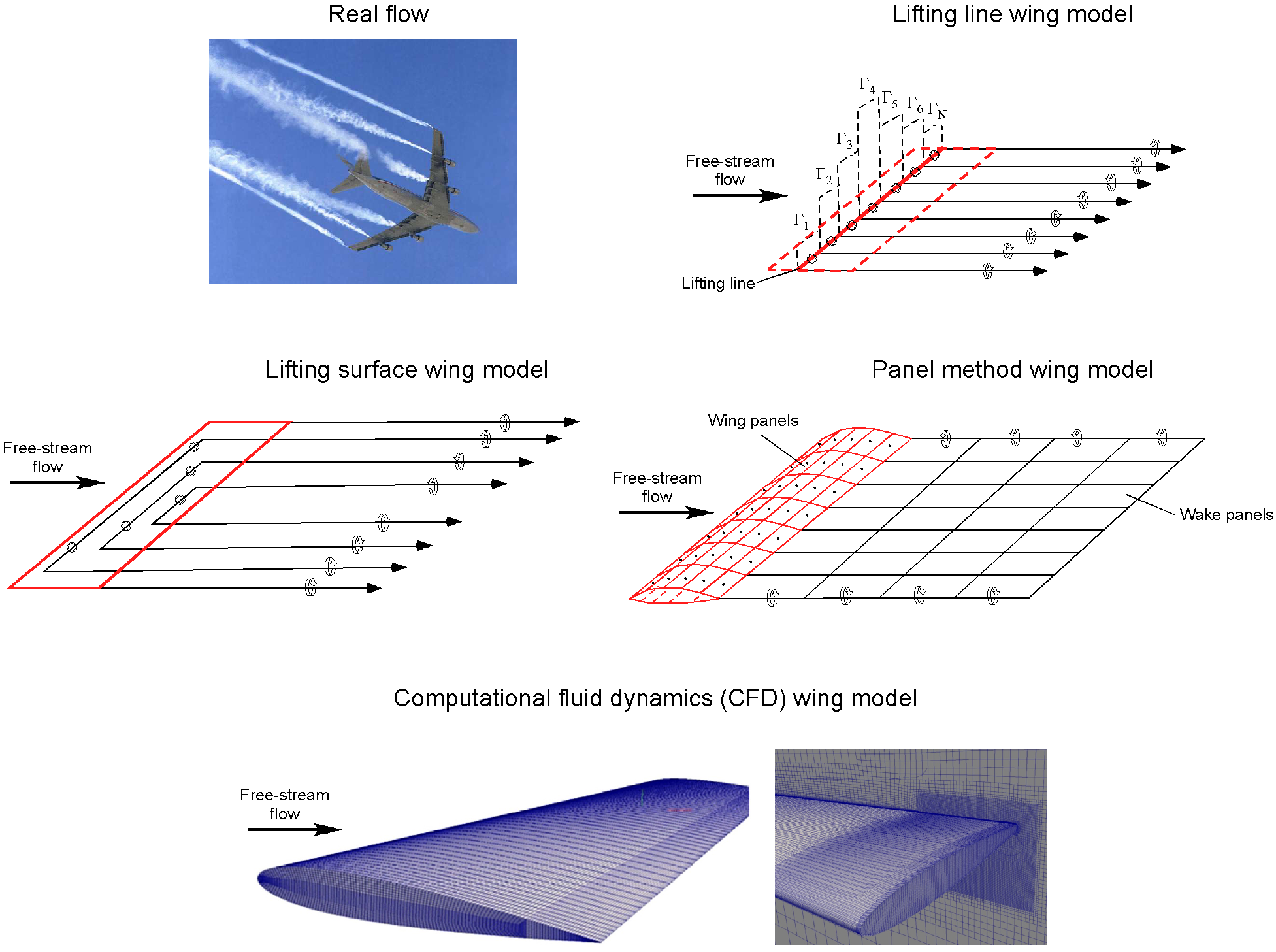
For example, the figure below illustrates a hierarchy of aerodynamic methods that can be used to model the actual flow, starting from lifting line theory, progressing through lifting surface theory to a panel method that also accounts for the effects of wing thickness, and ultimately to a full computational fluid dynamics (CFD) model. Each technique is accompanied by a corresponding increase in fidelity, as well as an increase in execution time and computational cost. Whether the problem is aerodynamics or otherwise, the idea is often to start with a more straightforward method to get some initial understanding of the problem at a relatively low cost and then progress to a more complex model with higher fidelity for the final calculations. For example, a CFD calculation may take up to five orders of magnitude more time and cost than the lifting line theory.

Verification and Validation

Inevitably, the outcomes from any model (i.e., the computed results) would be checked to make sure that they make sense, such as by comparing them with measurements, i.e., to establish how well the model works, a process called verification and validation or “V & V.” If the outcomes are positive, then the process inevitably also involves checking it for different input scenarios to ensure that the model predicts what it needs to predict and for the right reason. However, the process may conclude that the results do not agree. The V & V of all mathematical models is critically important, especially if such models are to be used in the design process. Confidence in the design tools being used is critical if the design is to prove viable or successful.

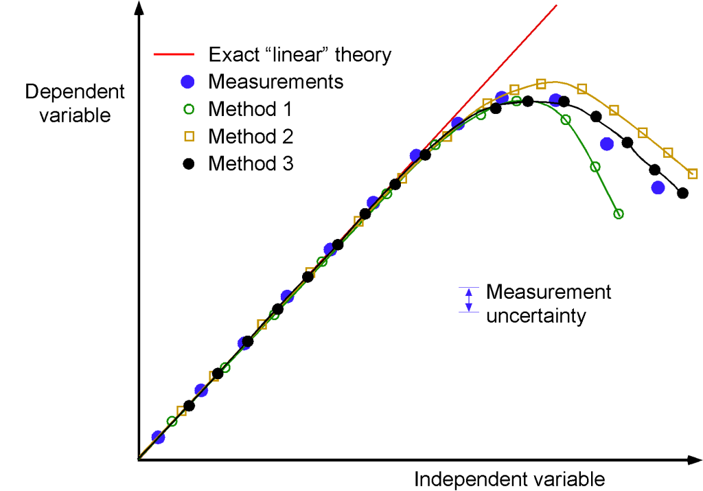
An example is shown in the figure below, where predictions from four mathematical models (i.e., different competing methods or theories) are compared with measurements. The question is: Which mathematical model performs best in comparison to the measurements? All methods work reasonably well over specific ranges, but one or more may be more effective than the others. The exact theory fails for higher values of the independent variable. Subjectively, Method 3 compares best to the measurement points. However, when measurement uncertainty is accounted for, Methods 1 and 2 may be equally effective in predicting their values. Unfortunately, in this case, the final answer as to the “best” model may be in the eye of the beholder!

Another issue to examine is ensuring that the best method predicts behavior for the right reason, which may require additional measurements and/or analysis to provide a comprehensive answer. Predicting the correct outcome for the wrong reason is not a verification or validation of the method. Indeed, some may argue that such models cannot be validated, only disproved, i.e., the essence of Popper’s falsification principle.

Finally, these equations (i.e., the “model,” in general) can be used to analyze similar problems of interest, such as in a parametric study where one quantity is varied using the model to establish the corresponding effects on the other quantities. Such parametric studies, utilizing mathematical and/or numerical models, are crucial in engineering design. For example, a particular combination of parameters may be sought to optimize the system performance or for another reason. However, it should always be remembered that no mathematical description of a physical problem can be perfect for its behavior. It can only be an approximation whose accuracy depends on how diligently the model is set up, including the nature of the assumptions and approximations.

Multi-Disciplinary Problems

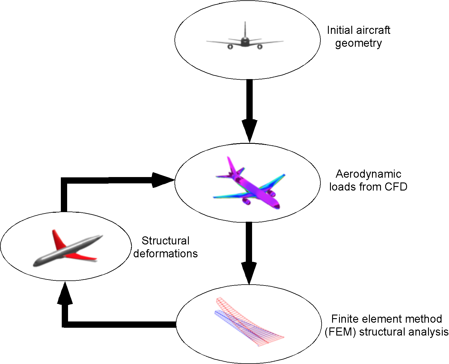
As previously discussed, aircraft and spacecraft structures are composed of lightweight, thin-walled elements, including various beams, columns, shafts, plates, and shells. All must be modeled in aggregate with aerodynamics using a multidisciplinary approach, as illustrated in the figure below. Coupling aerodynamics with the structures and structural dynamics is called aeroelasticity because the action of the aerodynamic loads elastically deforms the structure, which in turn feeds back to the aerodynamic loads. Combining models of aerodynamics and structural loads and deformations typically requires an iterative approach, which significantly increases computational time and overall effort.

Like aerodynamics, the governing equations of structural elasticity comprise sets of partial differential equations. Computational Fluid Dynamics (CFD) can help predict detailed aerodynamic loads if sufficient computing power is available, i.e., sufficient memory and execution speed. For the structure, the finite element method (FEM) is usually necessary to predict the behavior of complex structural geometries. The FEM is highly developed and sophisticated enough to handle almost any aerospace structure, but, like CFD, it also requires significant computing power. Sometimes, subsets of the governing equations may be sufficient to expedite the computational process, depending on the assumptions and approximations that can be justified, such as small displacements or isotropic structural properties.

Flutter is a form of aeroelasticity, a potentially catastrophic dynamic phenomenon that can occur with the flexible structures of aircraft and spacecraft. Flutter usually occurs when the forces created on an object cause it to displace or deform, elastically return to its original position, but also overshoot and then repeat the process, beginning to oscillate. This is a dynamic process that requires an inherently coupled aerodynamic and structural dynamic solution process. If the forces subsequently increase in magnitude, the oscillations also increase until the object eventually fails structurally; for example, the tail or a wing may break off during flight. Therefore, flutter must be avoided, and great efforts must be undertaken to ensure a flight vehicle is flutter-free. Unfortunately, flutter can still occur on flight vehicles, and it can also happen with buildings, bridges, and other flexible objects exposed to the wind.

Problem-Solving Process

The figure below illustrates that a general procedure for solving a physical problem typically involves several steps. The steps are not unique and will vary from problem to problem, but the iterative process is typical of all aspects of design, particularly for flight vehicles. The process involves numerous specialized activities and inevitably requires a considerable amount of time.

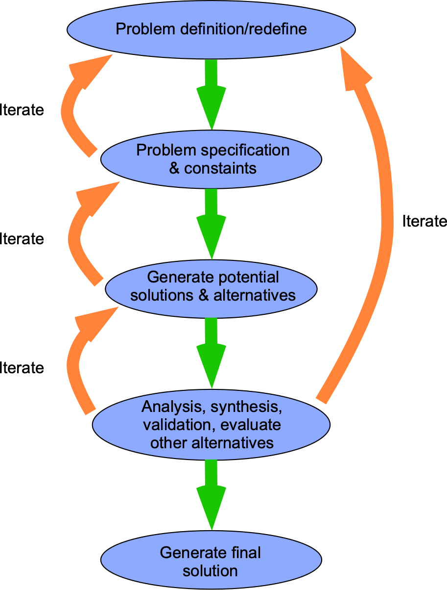
1. Specify or define and then describe the nature of the physical problem. This can often be done relatively quickly using an appropriately annotated sketch. For an aerodynamic problem, the annotations could include the size and shape of a control volume, the general flow directions, and the specifications of relevant boundary conditions.

2. Mathematically specify any relevant known boundary conditions, such as upstream freestream conditions. On the surface of a solid body placed in a flow, the flow would not pass through that body; therefore, another boundary condition is that the flow is parallel to the body surface.

3. Determine the primary form of the required model, i.e., whether an integral or differential approach is necessary. For example, if detailed properties are needed at all points, an integral approach is unlikely to be suitable, and the problem should be addressed using a differential model.

4. For aerodynamic problems, decide whether an Eulerian or Lagrangian flow model is required, i.e., whether the aerodynamic behavior at a fixed point or over a volume in space is needed or whether the identical fluid particles need to be tracked as they move through the flow.

5. Make any justifiable assumptions about the problem. The idea here is to take the actual physical problem and derive a simplified but still relevant mathematical version of the physical problem. By drawing on experience or from experiments on similar problems, it may be possible to make reasonable assumptions. For example, in aerodynamic problems, it may be possible to assume that the flow is steady and/or predominantly two-dimensional, which usually results in considerable simplifications of the mathematics. These assumptions are then used to help develop the appropriate governing equations for the model.

6. Apply the conservation principles to establish the mathematical form of the model that describes the physical problem. Because there are three physical principles to invoke (i.e., mass, momentum, and energy), most problems will involve three governing equations. However, auxiliary equations (e.g., an equation of state) may also be needed. These equations then need to be solved consistently and concurrently.

7. Conduct the solution process, where the relevant equations are solved to obtain the desired physical quantities, such as velocities and pressures, as needed for flow problems. In some cases, the equations may be solved analytically in closed form, meaning that the resulting solutions are purely mathematical and involve the creation of final sets of descriptive equations. The equations will likely need to be solved numerically; that is, a computer program must be written with numerical outputs.

8. Verify and validate the model to determine its accuracy and correctness, a process often referred to as “V&V.” In this process, predicted outcomes are used to assess how well the model represents the desired physical behavior. The model’s validity can be established by comparing the results with existing measurements, if such measurements are available or can be conducted, as shown in the figure below.

This step is essential in aerodynamic modeling and is one reason wind tunnels are critical in understanding all types of aerodynamic flows. If experimental data are unavailable, other theories can sometimes be used for validation; however, validation is rarely conducted without reference to appropriate measurements. In all cases, experience and good judgment must be used to establish that the predictive credibility of the model has been obtained. This is rarely a test that one person can objectively conduct, as confirmational bias, also known as confirmation bias, can play a role.^[3]

9. Enhance the model’s capabilities to broaden its scope. As experience is gained in the validation process regarding what the model predicts adequately and what it does not, the limitations and assumptions within the model can be progressively removed, or other enhancements can be made. For example, extending the range of validity of an aerodynamic model may be possible by incorporating unsteady effects or by accounting for turbulence. In a structural model, it may be necessary to include nonlinear effects, such as those from large deflections.

10. Finally, balance the model’s complexities and capabilities against the time and cost of obtaining solutions from the model. In this case, questions will have to be asked about how the model will be used and whether the full fidelity of the model is needed. For example, the need to model compressibility effects in the flow might not be required if the problem is restricted to low Mach numbers. Furthermore, if the model is to be used exclusively for research, then computational time and cost will be less crucial than for use in the industry, where a short turnaround time is always needed.

Generalization of Data & Data Fitting

The ability to generalize data from one or more sources, whether experiments or computations, is an essential skill for effective engineering modeling. Many engineering problems are too complex to be adequately represented by theoretical models in the form of parsimonious equations. Therefore, mathematical models used for design at the system level are often empirical or semi-empirical, meaning that they are either based entirely on observations from experiments, i.e., based on “curve-fits,” or based primarily on theory but augmented by key data taken from experiments, which is referred to as a semi-empirical model. Semi-empirical models are standard in engineering analyses, as illustrated in the figure below. Dimensional analysis is also helpful here, as the entire domain can be more readily generalized if the measured data from different experiments are expressed and compared in terms of dimensionless parameters or groupings, such as the Reynolds number, Mach number, and force coefficients.

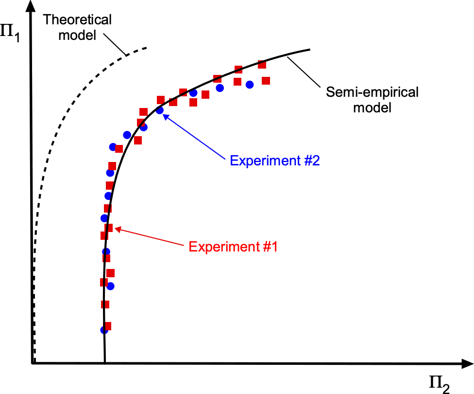
For example, a pure theoretical model may be of the form

(1)  

which may show good qualitative agreement with measurements but not quantitative agreement. However, a semi-empirical model of the form

(2)  

may show much better agreement with experiments where the numerical values of and are semi-empirical coefficients derived by matching the available data in some manner, such as based on a least-squares fit. Experienced modelers may even establish the coefficient based on subjective assessments, but this is not recommended. Nevertheless, the measurements used to establish the semi-empirical model must be comprehensive enough to ensure that reasonable predictive confidence has been achieved. Finally, any reasonable application of the scientific method will limit predictions to within the bounds of the measurements; significant extrapolation (either upward or downward) using a semi-empirical model is always a dangerous practice.

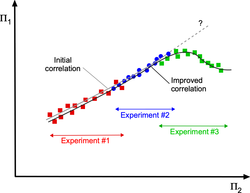
It is rarely possible to cover the entire domain of the parameter space in one single experiment. In this regard, not all test facilities are created equally. One experiment may cover a limited range of the domain, while another experiment may cover a different range, possibly with some overlap, as illustrated in the figure below. Each experiment may be inadequate in establishing any useful, robust, causal correlation. However, a semi-empirical model can show a more robust and positive correlation if the data is taken collectively and used intelligently in the generalization process.

Repetition of experiments is always a good practice, which can also benefit from advancements in measurement technologies. Indeed, the scientific method requires that any one experiment can only be fully trusted once it has been independently repeated and the results confirmed.  Unfortunately, repeating experiments is often difficult to justify based on cost, time, or both. Inherent differences in the testing facilities can also be a consideration, such as wind tunnel interference effects and measurement limitations. However, the logical rationalization here from the perspective of the scientific method is that the ability to make better measurements will lead to lower errors and inaccuracies in the acquired data. Therefore, a stronger causal correlation is likely to be demonstrated, and a greater predictive confidence can then be gained. Nevertheless, for any given dataset, there is always considerable uncertainty in extrapolation beyond the range of the measured data.

Over time, new experiments on a given problem are inevitably conducted, and some may be ambitious enough to extend the domain’s range. Such data may confirm existing trends or be disruptive, suggesting a different correlation, as shown in the figure above. On the one hand, such disruptive data lead to improved correlation and more confident mathematical models, which show enhanced predictive confidence at the system level. On the other hand, predictions at the system level may be worse, in which case one can suspect that one modeling error has previously acted to cancel another, i.e., duo mala faciunt unum bonum, and so point to further modeling deficiencies. The stakes in such outcomes are high, as the validity of the entire system model can be called into question until the weaknesses in other parts of the model are identified and corrected. In this regard, complex models, especially those with significant empiricism, can remain perpetually tentative until more and/or confirmatory measurements are obtained.

Ockham’s Razor – The KIS² Principle

One issue with complex engineering models for multidisciplinary aerospace applications is that significant empirical evidence may be required. Some physical problems are difficult to model without resorting to substantial empiricism, an unavoidable consequence of representing complex physical processes with parsimonious models that achieve practical levels of computational efficiency. In this regard, there is always a need to balance the complexity of the mathematical model against its predictive accuracy, while aiming to minimize variability and maximize intelligibility in the resulting simulations. For complex mathematical models, history has shown that predictive accuracy increases with increasing modeling complexity only up to a point where the cumulative uncertainties in the model’s components, particularly those with significant empirical foundations, begin to increase the “noise” in the predictions. Then, beyond a certain level of complexity, the predictive accuracy decreases again, the system exhibiting a classic “Ockham’s Hill,” as shown in the figure below.

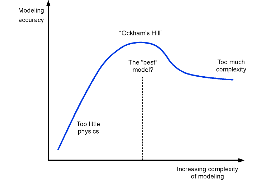
In this regard, it is essential to remember the principle of Ockham’s Razor, i.e., given two sets of solutions from methods of equivalent accuracy, one should side with the simpler or parsimonious method, i.e., Frustra fit per plura quod potest fieri per pauciora. This approach is sometimes called the KISS or KIS2 principle, which means “Keep it Short and simple.” Ernst Mach was also an advocate of a similar principle, which he called the “Principle of Economy,” stating: “Scientists must use the simplest means of arriving at their results and exclude everything not perceived by the senses.” The message is evident in that the goal for engineers is to strike a balance between modeling complexity and predictive fidelity, something that cannot be achieved solely through careful, systematic validation studies, but also requires a degree of common sense.

Approaching Homework Problems

The skills and abilities to solve real engineering problems develop from the exemplar problems encountered in the classroom. To this end, budding engineers must first excel at solving homework problems. Results generated in homework problems may be single numbers, tables, or graphs in any or all combinations that must be adequately presented. Below are some general guidelines to help new students tackle homework problems and build up the skills they need to learn as engineers.

Homework is NOT a quiz!

The idea of homework for engineering students is to begin learning the process of solving real-world problems, which becomes a lifelong endeavor for an engineer. Homework problems expand upon what can be done in the classroom, which are usually simpler and straightforward. When doing homework, students can utilize all the available resources, including exemplar problems and solutions provided in the textbook or e-book, many of which are former exam or quiz questions. Students should use these exemplars to help them understand the process of solving similar problems that may come up on homework and future exams.

If you are a student and need help understanding how to approach a specific homework problem, ask your instructor before or after class, during office hours, or by email. Refrain from guessing! Also, do not copy down former “solutions” to similar problems and present them as your own – use the exemplar solutions to understand the process of solving the current homework questions, then write out your own solutions. Finally, do not assume that the current question(s) is (are) exactly the same as a previous question you may have seen; submitting the correct answer to the wrong homework problem will not have a good outcome.

A student’s homework score may account for a significant portion of their total grade in an engineering course. This fraction reflects the importance that instructors place on learning the methods and techniques for solving engineering problems, as well as developing and maintaining other essential skills, including presentation formats, time management, MATLAB use, and graph drawing, among others. Remember that students may see exam questions that are very similar to homework questions, which are often easier! Therefore, if students approach homework problems seriously and dedicate the required time to understanding the processes of solving them, they can expect to perform well on the exams. History speaks for itself in this regard.

Pointers for Doing Good Homework

Preparations

1. 1. Review the homework problem set as soon as the professor or course instructor assigns it. Remember: Start working on the problem set early! Time management is essential.
   2. Don’t guess! Homework is not a quiz. It is a learning exercise, so don’t consider it a quiz or exam.
   3. If you need help with the homework questions, attend the professor’s, instructor’s, or TA’s office hours. Come prepared and ask specific questions; other students may be waiting to ask their questions.
   4. Don’t post your homework problems online, hoping that someone in cyberspace knows better than the person who wrote the question. Ask the professor or whoever wrote the problem(s) for advice.
   5. Check whether a similar problem is addressed in the textbook, e-book, or notes. Review old problem sets and their solutions – professors usually make them available to students.
   6. Meet with other students, your study group, the TA, the grader, or anyone else to try to understand the problem and potential solution. One effective learning method is for one student in a study group, for example, to try to teach the solution method to the others.

Starting on the Problems

1. 1. Based on the information provided, state the problem statement briefly and concisely. It is often helpful to restate the information in the question, clearly and straightforwardly stating what is known and what is not.
   2. If appropriate, draw a sketch or schematic of the problem/approach. In most cases, an annotated sketch of the physical problem will help you decide the nature of the mathematical model that needs to be adopted, e.g., control volume approach or otherwise.
   3. Write down the appropriate mathematical equations necessary to solve the problem. These equations should not be expected to be given in the homework problem, at least not in all cases. Choosing (or deriving) a set of simpler equations from a broader, more general set of governing equations may be necessary.
   4. List and develop any simplifying assumptions appropriate to the problem. Sometimes, the assumptions will be specified; others may be left as part of the problem. For some more challenging problems, it may not be apparent initially what assumptions are needed. Several attempts may be necessary until the correct assumptions can be confirmed and verified.

Working the Problems

1. 1. 1. Be sure to work carefully and systematically through each problem. It is better to work slowly but get the correct answer than to work faster and make silly mistakes.
      2. Complete the analysis in algebraic form (i.e., equations with symbols and variables) before substituting the specific numerical values. Sometimes, the answer will be presented as an equation rather than a numerical value.
      3. Substitute known numerical values (using a consistent set of engineering units) to obtain a numerical answer or answers. If the problem is given in SI units, it is best to work it entirely in SI units; conversely, if it is given in US customary units (USC units), then work it entirely in USC units. For example, switching back and forth between USC and SI is inadvisable because this approach is often a source of mistakes and numerical errors.
      4. All numerical answers must have appropriate units unless they are in non-dimensional form. Always double-check the engineering units of the solution (s). Units should be used consistently throughout, ideally in base units.
      5. Check that the number of significant digits in the answer(s) is/are consistent with the given data. For example, if you are given information to 3 significant digits, it would not be appropriate to calculate your final results to 5 significant digits. However, it is good practice to round off numerical values at the end of the problem.
      6. Review the answer(s) for correctness. In some cases, it will be evident if the result is wrong; it may be challenging in other cases. In many cases, the question is: Does that result seem physically correct? Check with someone else if in doubt, such as a course instructor.
      7. Draw a box around the final answer to clarify that this is your definitive answer. The answer will often be an equation (or formula) or a number, but it could also be a table or a graph. You do not need to draw a box around tables or graphs.
      8. Import the results into the appropriate software if a graph is needed. Never draw graphs freehand!! Use MATLAB, Excel, or your favorite graphing program. Kaleidagraph was used for many of the plots in this e-book. As appropriate, all graphs need to have proper legends, labels, and other annotations.

Submission

1. 1. Your submitted homework must be neat and easy to follow. You will also need to follow the submission rules. For example, you may need to use squared engineering paper, include your name and student identification number on each page, and staple your pages together, among other requirements. If not, you will likely get less credit regardless of the correct solution. In the industry, great emphasis is placed on the clarity and presentation of reports and papers; for the same reason, clarity in homework is a good place to start.
   2. Write down clearly and unambiguously the names of the student(s) you worked with on the homework, if any. Working with others is acceptable, but you should submit your OWN answers to the questions. For example, you may state, “I cross-checked my final answers with John and Kevin, and my answers agreed with theirs.”
   3. Be sure to submit your homework on time and follow your professor’s requirements, such as submitting it on paper or as a file upload.

All those Equations!

In engineering (or any scientific field), students do not have to memorize hundreds of equations or formulas. The questions and concerns from new students of the field inevitably soon start to flow, such as: ” What equation do I use?” or “Where do I find the equation?” or “What is this symbol in this equation?” or “Where do I get the solution to this integral?” Such questions are natural, and guidance from experienced engineers and professors is essential. As taught in many educational contexts, the “plug and chug” paradigm of plugging a numerical value into some equation and chugging out an answer is a surefire recipe for disaster in actual engineering problem-solving. Bona fide engineering students need to learn to do much better.

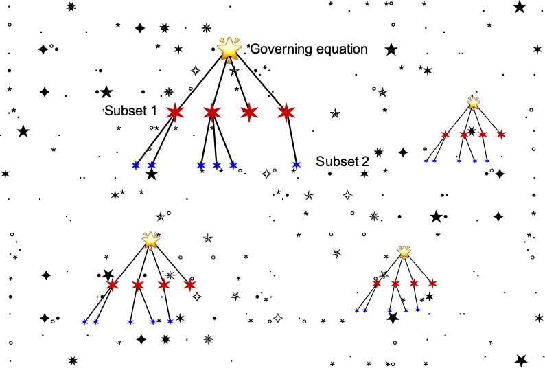
The number of equations in science and engineering could be as many as the number of stars in the galaxy! No exaggeration. As the figure below suggests, most successful engineers and professors remember the details of the biggest stars and the most general form of the equations, or the “governing” equations. They also understand the concepts and have completed enough problems to know how to reduce and simplify equations under certain assumptions and conditions, producing subsets of equations with specific applicability to the problem at hand. The equations they can’t remember can usually be derived! The governing equations can then be adapted and applied successfully to various situations by grasping the underlying concepts, rather than memorizing dozens of problem-specific equations. Science and engineering are not a memory game.

The risk in memorizing without understanding is that the wrong equation (or equations) are applied, so the answer obtained is inevitably wrong, too, which is always a disastrous outcome in engineering problem-solving. Therefore, rather than relying on rote memorization or searching for a specific formula that may or may not be applicable, understanding the fundamental principles enables engineers to derive and apply the relevant equations to particular problems. While some foundational equations may be readily accessible, the focus should still be on understanding the underlying physical principles and fundamental concepts expressed by these equations, appreciating the meaning of all the terms, and rationalizing the best solution strategies for them.

Moreover, with access to the Internet, students can readily access information and resources to find the more general form of the equation(s) that might be needed. Unfortunately, the Internet is riddled with opinionated absurdity, especially when it comes to aerospace engineering topics, so using authoritative resources is crucial. Utilizing selective online resources, as well as peer-reviewed publications, textbooks, and sanctioned computational tools, can help new students and practicing engineers retrieve or verify specific equations and/or solution methods when needed. Labora sapienter, non strenue.

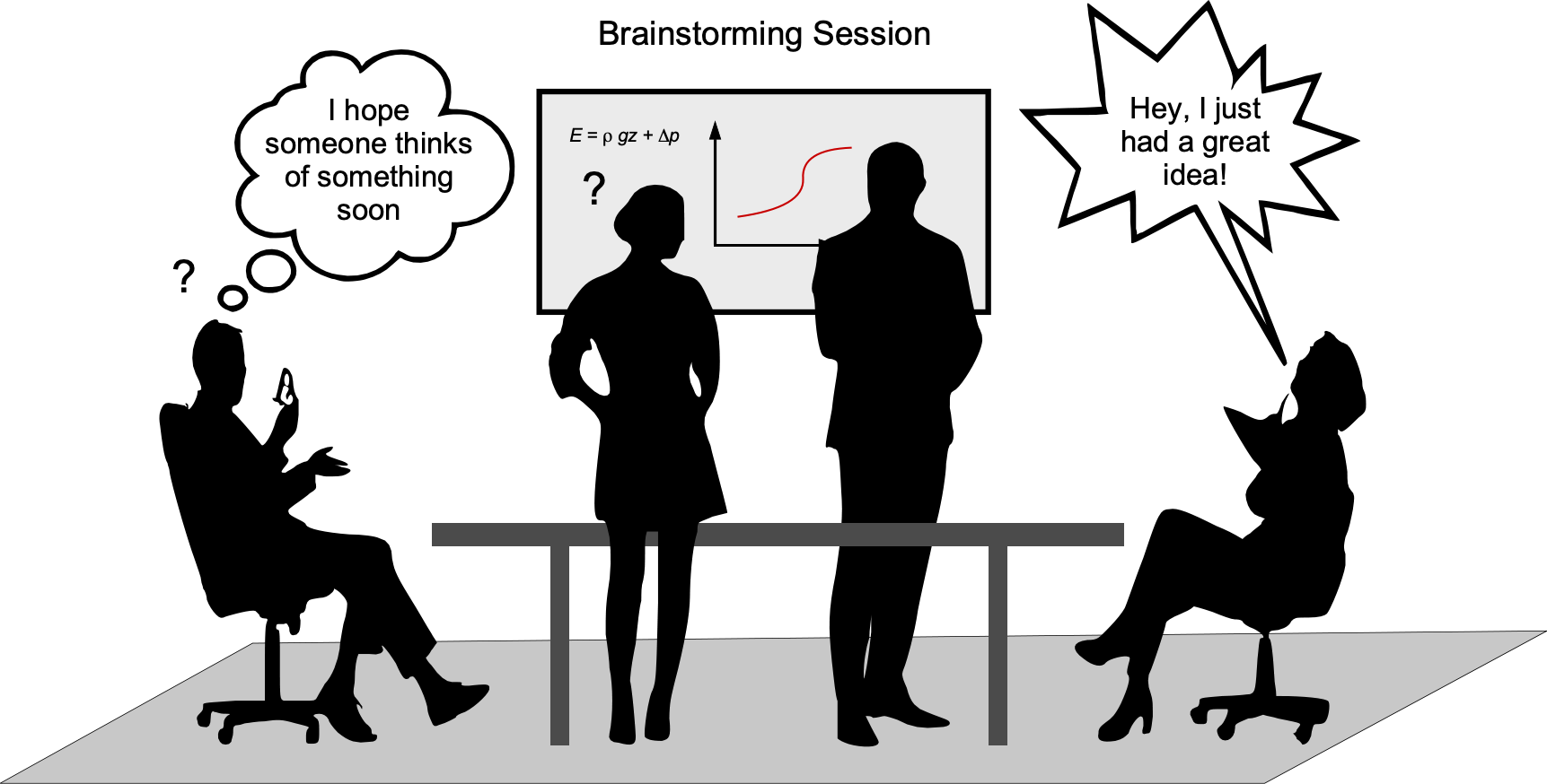
What is Brainstorming?

Brainstorming is an informal yet highly effective approach to problem-solving in engineering, which also works for homework problems. Usually conducted with a small group of engineers or students and a single moderator, brainstorming encourages all participants to think laterally and develop ideas that might initially seem unusual or even sound slightly crazy!

A group of five to seven people is usually the most influential, with a mix of experienced and less experienced engineers. The moderator should be someone other than the chief, lead engineer, or an engineer in management, and the group itself should select the moderator. The group should comprise individuals from various technical disciplines to foster and develop the most effective and productive brainstorming environment. Excellent ideas may ultimately emerge from engineers who see an avenue of opportunity in a discipline different from their own and so approach the problem with a fresh perspective. Some of these ideas may be developed into a rational basis for engineering problem-solving, often following a new or innovative path that nobody else had considered previously. The basic idea is to encourage all participants to think “outside the box,” be creative, and divert their attention away from relying on their conventional wisdom to solve problems.

Brainstorming is often highly effective for solving complex engineering problems that require multidisciplinary approaches. The best ideas in a brainstorming session often emerge from less experienced engineers, who are less encumbered by conventional wisdom. Brainstorming is best conducted in an informal, relaxed environment away from the typical day-to-day work environment, often at a retreat location. Brainstorming can also be fun, an excellent environment for team building, and a way of getting to know other engineers outside one’s primary technical discipline or organization. It is not unusual for companies to collaborate on solving complex engineering problems in the aerospace field, and brainstorming sessions can foster more substantial inter-company dialogue, enabling everyone to work more effectively together.

For brainstorming to be effective, all group members must be active participants, and personal criticism is inappropriate. Often, a quirky idea from one group member may seem nonsensical at first, but after discussion, a “aha!” or “I never thought of that!” moment can emerge. After the discussion, the group may buy into the idea. Alternatively, the idea may lead to a different revelation and a novel path to solving the problem that nobody had considered before.

To prepare for the brainstorming session, a location with minimal distractions must be identified. All phones and computers should be turned off, the doors should be locked, and a whiteboard should be available for writing down ideas. Everyone should have an opportunity to speak when they want to. The moderator must refrain from allowing any one member of the group to dominate the brainstorming session. At the end of the session, the group selects the best ideas and then proceeds, as needed, to follow up and pursue them. The history of engineering suggests that many of the best and most innovative ideas can come from brainstorming sessions.

Summary & Closure

Developing mathematical models to study and solve various engineering problems is an integral part of the field. However, the selection process must be conducted carefully and systematically to choose or develop the relevant governing equations that apply to the specific problem (or problems) of interest. In some cases, it may be possible to down-select the appropriate governing equations for a particular problem from more general forms of governing equations that are intended to apply to a broader range of conditions. In other cases, the governing equations may need to be developed from first principles.

Once a mathematical model or set of models has/have been developed, it is necessary to solve the equations to make predictions about the system being modeled. The solution process can involve analytical methods, such as closed-form solutions, or numerical methods, such as finite element, finite difference, or boundary element methods. The choice of solution method will depend on the nature of the problem, the available resources, and the desired accuracy of the solution. In all cases, justifying assumptions and/or approximations is necessary. In this regard, any reason may require reliance on outcomes from experiments, i.e., for verification and validation of the modeling. A combination of solution methods may often arrive at an acceptable solution. Additionally, post-processing and visualization techniques can aid in interpreting the results and behavior of the modeled system.