Airplane Equations of Motion

J. Gordon Leishman

doi:https://doi.org/10.15394/eaglepub.2022.1066.n27

37 Airplane Equations of Motion

Introduction

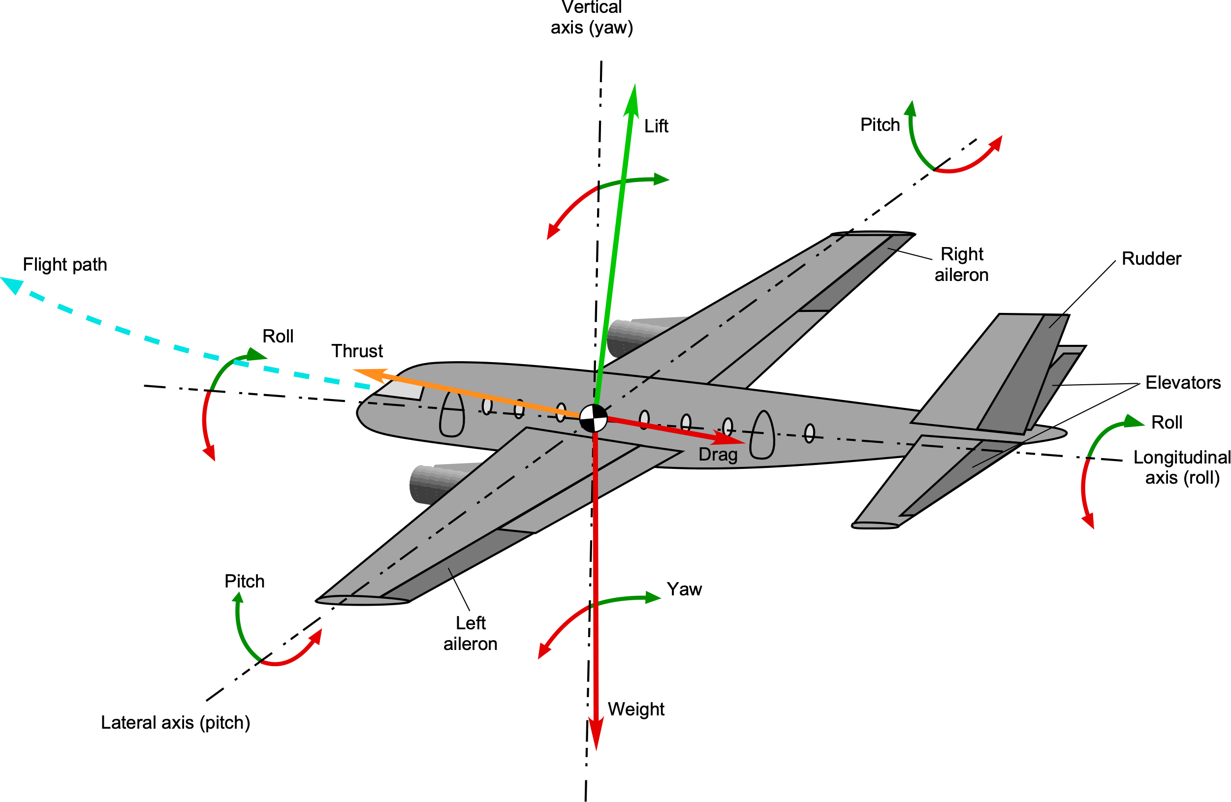
Unlike a two-dimensional terrestrial vehicle, an airplane can move along an almost infinite number of possible three-dimensional spatial paths. An airplane may undergo steady and/or accelerated motions along its pitch and/or roll and/or yaw axes, as shown in the figure below. In practice, however, any airplane’s flight path and attitude will be limited to values within its aerodynamic performance and structural stress envelopes. In this regard, not all airplanes are created equally, nor will they have unlimited flight capabilities. For example, the number of feasible flight paths possible with an airliner will not be the same as those for a jet fighter, nor would they be expected to be based on their design purpose.

An airplane can pitch, roll, yaw, and move about all three axes to follow an almost unlimited number of possible curvilinear flight paths.

To help analyze airplane motion and performance, the general equations of motion for an airplane in flight must be established. These equations help expose an airplane’s fundamental performance characteristics during steady flight and some cases of maneuvering flight, including turns and pull-ups. These results also help appreciate the factors that can, and inevitably will, limit the airplane’s flight capabilities, either aerodynamically, structurally, or both. Structural limits are usually defined in terms of a maneuvering flight envelope, which maps out the combinations of limiting airspeeds and maximum load factors within which the airplane can safely fly without causing a structural overload.

Learning Objectives

Know about the terminology and conventions used to describe the motion of an airplane, including its pitch, roll, and yaw.
Set up the equations for the forces on an airplane following a general flight path and when undergoing basic maneuvers.
Understand the meaning and significance of an airplane’s “load factor” and calculate the load factors in steady turns and pull-up maneuvers.
Appreciate the significance of a maneuvering envelope in terms of limiting airspeeds and allowable load factors.

Assumptions

To analyze an airplane in flight, the equations that describe its motion must first be set down in terms of lift, weight, drag, and propulsive force (i.e., thrust). The overall approach is relatively straightforward but requires the careful application of the principles of statics and dynamics. The objective is to describe the airplane’s movement through the atmosphere using equations that physically describe its curvilinear motion, thereby allowing its performance and other flight capabilities to be evaluated. In an initial analysis, the airplane can be replaced by a point mass at its center of gravity (c.g.) following a curvilinear flight path, as indicated in the figure below.^[1] The angle $\gamma$ is the flight path angle of the airplane relative to the Earth’s surface, and $\phi$ is the bank angle.

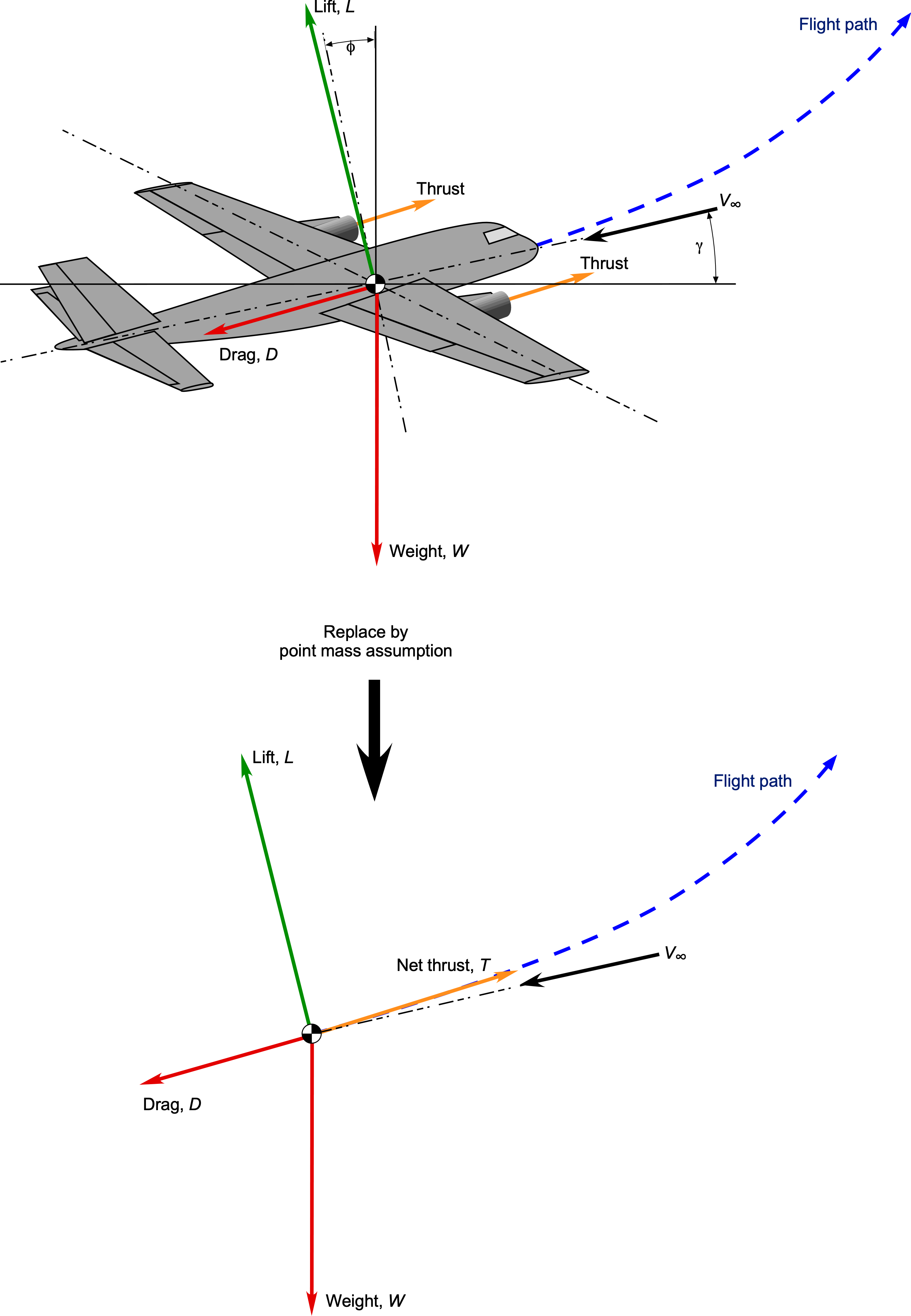
A point mass assumption for an airplane is a reasonable representation for an initial analysis.

The aerodynamics of the wings, empennage, airframe, etc., need not be considered in individual detail for a first-level analysis of the equations of motion but can be represented as total lift, drag, and pitching moments on the airplane. While the aerodynamic forces will act at an effective center of pressure location, it is initially convenient to colocate them at the center of gravity without considering any aerodynamic moments. Experience shows that the lift and drag of an entire airplane can also be analyzed with a high confidence level using a composite aerodynamic drag polar (i.e., the relationship between lift coefficient and drag coefficient) if this can be suitably obtained or even assumed.

As discussed earlier, the most common and representative drag polar for an airplane at subsonic flight speeds up to the point of wing stall is

(1) $\begin{equation*} C_D = \underbrace{ C_{D_{0}}}_{\begin{tabular}{c} \scriptsize Non-lifting \\[-3pt] \scriptsize drag \end{tabular}} + \underbrace{\frac{{C_L}^2}{\pi \, A\!R \, e}}_{\begin{tabular}{c} \scriptsize Induced \\[-3pt] \scriptsize drag \end{tabular}} = C_{D_{0}} + C_{D_{i}} \end{equation*}$

The first term in the preceding equation is the non-lifting profile/parasitic drag component, and the second term is the induced drag, with $A\!R$ being the aspect ratio of the wing and $e$ being Oswald’s efficiency factor for the airplane (i.e., $e < 1$ ). Polars are available for various airplanes or can be estimated based on historical data in cases where the polar may not be known, such as for preliminary design.

It is often convenient to have an analytic relationship between the $C_L$ and $C_D$ coefficients if general closed-form equations for thrust and or power for flight are to be determined. However, other methods may be used in some cases, such as a table look-up process, where the coefficients may be specified as discrete values as functions of the angle of attack and Mach number, including the effects of wave drag. The needed values between the discrete entries in the table can be readily obtained by interpolation, and the desired results for thrust and/or power required are then obtained by numerical methods.

At first, the details of the propulsion system need not be considered, but it must be recognized that not all propulsion systems will have the same characteristics and/or limitations. Nevertheless, the propulsive system must eventually be considered for all forms of flight analysis, at the very least in terms of thrust produced and/or power available, as well as the fuel consumption, i.e., the engine’s fuel efficiency in producing a given amount of thrust or power.

In summary, it is possible to proceed to analyze the motion of an airplane by summarizing the fundamental assumptions that will allow the development of the equations of motion and expose the primary influencing parameters and their dependencies:

The distributed weight of the airplane can be replaced by a center of gravity (c.g.) location, and the entire weight can be assumed to be at the c.g., i.e., a point mass assumption.
The aerodynamic representation uses integrated quantities in terms of lift coefficient $C_L$ and drag coefficient $C_D$ in the form of a drag polar.
The propulsive device is considered in terms of its thrust production (or power supplied) and its specific fuel consumption. While aircraft engines run more or less at full throttle, a dependency on the throttle setting may also be specified.

Curvilinear Flight in a Vertical Plane

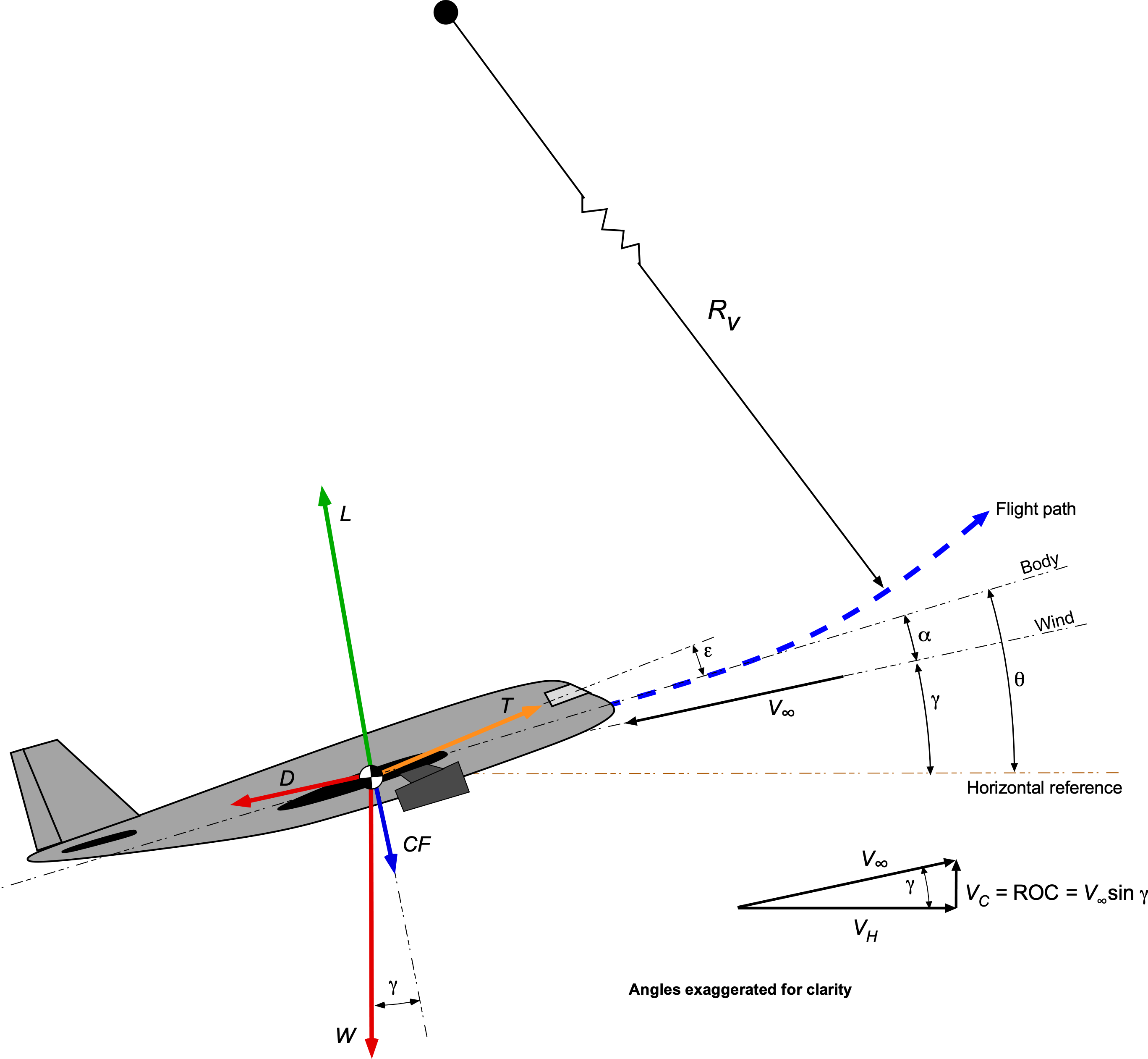
The figure below shows an airplane in curvilinear flight relative to the surface of the Earth (assumed here as the horizontal reference), where $\gamma$ can be viewed as the instantaneous flight path angle. The four (resultant) forces involved in the flight are the lift $L$ , weight $W$ , drag $D$ , and thrust $T$ , as also shown in the figure below. Notice that the angles in the diagram are exaggerated for clarity compared to a typical climb, but the airplane could be maneuvering, i.e., accelerating. For descending flight, the value of $\gamma$ would, of course, be negative. In summary, then

The free-stream or airspeed vector is given by $V_{\infty}$ .
The lift is given the symbol $L$ and, by definition, acts perpendicular to $V_{\infty}$ .
The drag is given the symbol $D$ and acts in a direction parallel to $V_{\infty}$ .
The weight $W$ acts at the center of gravity (c.g.) and toward the center of the Earth.
The angle $\theta$ is the pitch angle of the airplane relative to a body axis datum.
The angle $\gamma$ is the flight path angle of the airplane relative to the Earth’s surface.
The angle $\alpha$ is the airplane’s angle of attack relative to $V_{\infty}$ .
The angle $\epsilon$ denotes the line of action of the propulsive thrust force, which may be inclined relative to the body axis (for various reasons).
The angle $\phi$ is the airplane’s bank angle, positive in a right bank (right-wing low). In a vertical plane, the wings would be level, so $\phi = 0$ .

An airplane in a nose-up condition following a rectilinear flight path.

In the direction parallel to the flight path, then

(2) $\begin{equation*} F_{\parallel} = T \cos \epsilon - D - W \sin \gamma \end{equation*}$

The acceleration parallel to the flight path will be

(3) $\begin{equation*} a_{\parallel} = \frac{d V_{\infty}}{dt} \end{equation*}$

and so

(4) $\begin{equation*} F_{\parallel} = \left(\frac{W}{g}\right) a_{\parallel} \end{equation*}$

where the “mass” of the airplane $M = W/g$ . Therefore, the equation of motion is

(5) $\begin{equation*} \left( \frac{W}{g} \right) \frac{d V_{\infty}}{dt} = T \cos \epsilon - D - W \sin \gamma \end{equation*}$

In the direction perpendicular to the flight path, the forces are

(6) $\begin{equation*} F_{\perp} = L \cos \phi + T \sin \epsilon \cos \phi - W \cos \gamma \end{equation*}$

where $\phi$ is the bank angle. For the wings-level condition ( $\phi = 0$ ) then

(7) $\begin{equation*} F_{\perp} = L + T \sin \epsilon - W \cos \gamma \end{equation*}$

The centripetal^[2] acceleration perpendicular to the flight path is

(8) $\begin{equation*} a_{\perp} = \frac{V_{\infty}^2}{R_v} \end{equation*}$

where $R_v$ will be the instantaneous radius of curvature of the flight path in the vertical plane. Notice that the centrifugal^[3] force (CF) acts outward, which is an inertial force in the direction opposite to the centripetal acceleration vector. Therefore, because $F_{\perp} = (W/g) \, a_{\perp}$ , then for the wings level condition, the equation of motion is

(9) $\begin{equation*} \left(\frac{W}{g}\right) \frac{V_{\infty}^2}{R_v} = L + T \sin \epsilon - W \cos \gamma \end{equation*}$

The preceding equations of motion are general and will apply to any flight path in a vertical plane.

What is the difference between centripetal acceleration and centrifugal force?

The centripetal acceleration is the acceleration experienced by an object moving in a curvilinear or circular path. It is directed toward the center of curvature of the path and is the acceleration needed to keep the object of a given mass from otherwise following a straight path (i.e., Newton’s 1st law). Centripetal accelerations must be caused by a force, which is required to maintain the object’s curvilinear or circular motion (i.e., Newton’s 2nd law). This force can be provided by various sources, such as tension in a string, gravitational attraction, the tires of a car driving down the road, or the lift on the wing of an airplane during flight. The centrifugal force is an inertial reaction force, often called a “virtual” force, that acts on an object moving in a curvilinear path in a direction outward and away from the center of rotation (i.e., Newton’s 3rd law).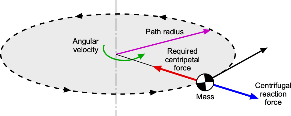

Steady Climb

Under the conditions where the airplane is in a steady climb with no accelerations parallel or perpendicular to the flight path, then $a_{\parallel} = a_{\perp} = 0$ , so for horizontal equilibrium, then

(10) $\begin{equation*} T \cos \epsilon - D - W \sin \gamma = 0 \end{equation*}$

and for vertical equilibrium, then

(11) $\begin{equation*} L + T \sin \epsilon - W \cos \gamma = 0 \end{equation*}$

When $\epsilon = 0$ , which is generally small anyway and so a reasonable assumption to make, then

(12) $\begin{equation*} T - D = W \sin \gamma \end{equation*}$

and

(13) $\begin{equation*} L = W \cos \gamma \end{equation*}$

so the climb angle, $\gamma$ , is given by

(14) $\begin{equation*} \gamma = \tan^{-1} \left( \dfrac{T - D}{L} \right) \approx \tan^{-1} \left( \dfrac{T - D}{W} \right) \end{equation*}$

The rate of climb (ROC), denoted by $V_c$ , is then

(15) $\begin{equation*} V_c = V_{\infty} \sin \gamma \end{equation*}$

Notice that the ROC will be maximized under high thrust, low drag, and low weight conditions.

Straight & Level Flight

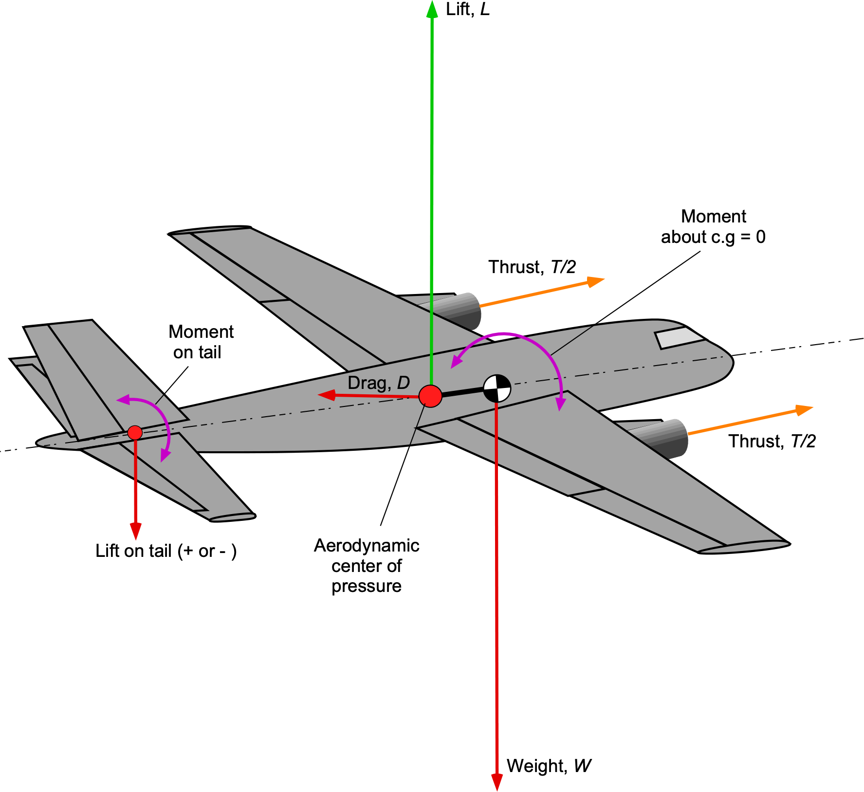
In this condition, the airplane is in pitching, rolling, and yawing moment equilibrium, i.e., operating in balanced or “trimmed” flight such that the net sum of all of the forces and moments about the c.g. are zero. The four (resultant) forces involved in the flight are the lift $L$ , weight $W$ , drag $D$ , and thrust $T$ , as shown in the figure below. Most airplanes will spend much of their flight time in straight-and-level, unaccelerated flight conditions. In this case, the forces on the airplane are in balance, i.e., in a static equilibrium. In this figure, the aerodynamic forces are assumed to act at a center of pressure location, in which case they will create a moment about the c.g.

In the level flight trim condition, the forces and moments on the airplane will be in perfect balance.

For horizontal equilibrium, then

(16) $\begin{equation*} T \cos \epsilon - D = 0 \end{equation*}$

and for vertical equilibrium

(17) $\begin{equation*} L + T \sin \epsilon - W = 0 \end{equation*}$

If $\epsilon = 0$ , then

(18) $\begin{equation*} L = W \quad \mbox{and} \quad D = T \end{equation*}$

In the equilibrium condition, i.e., the airplane is flying in trim, the sum of the moments on the airplane about each of the three axes will also be zero, i.e.,

(19) $\begin{equation*} \displaystyle{ \sum_{\rm pitch} = \sum_{\rm roll} = \sum_{\rm yaw} = 0} \end{equation*}$

Check Your Understanding #1 – Steady level flight trim

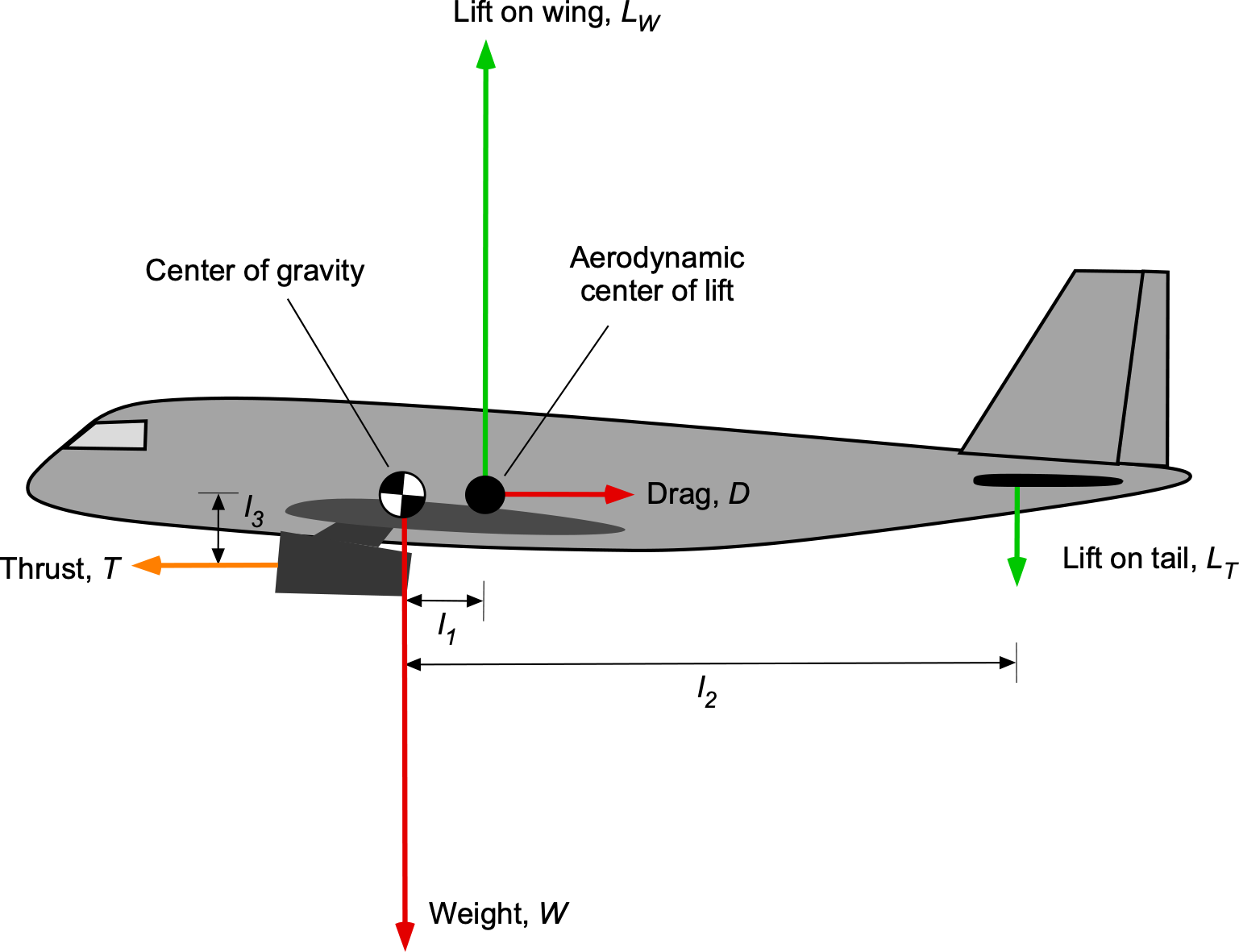
Consider the airplane in the figure shown below. The airplane’s weight can be assumed to act at its center of gravity. In the first instance, assume that the thrust/pitch coupling and this moment about the center of gravity is zero, i.e., $l_3 = 0$ . What must be the balance of forces and moments on the airplane in straight and level, unaccelerated flight at a constant airspeed? If $L_T = a \, L_W$ where $a$ is a constant, what is the value of $L_W$ ? Find also the relationship between $l_2$ and $l_1$ . If the thrust/pitch coupling effect is now included, how does this affect the moment trim?

Show solution/hide solution.

For vertical force equilibrium without the consideration of thrust/pitch coupling, then

$L_W - L_T = W$

We are given that $L_T = a \, L_W$ , so that

$L_W - a \, L_W = W$

or by algebraic rearrangement, then

$L_W ( 1- a ) = W$

Therefore,

$L_W = \frac{W}{(1 - a)}$

For pitching moment equilibrium, then

$L_W \, l_1 = L_T \, l_2 = a \, L_W \, l_2$

so the relationship between $l_2$ and $l_1$ is

$\frac{l_1}{l_2} = a$

If the thrust/pitch coupling effect is now considered, then for the pitching moment trim

$L_W \, l_1 - L_T \, l_2 + T \, l_3 = 0$

If $L_T = a \, L_W$ , then

$L_W \, l_1 - a \, L_W \, l_2 + T \, l_3 = L_W \left( l_1 - a \, l_2 \right) + T \, l_3 = 0$

Therefore, in this case, the fraction of the lift that the tail must produce

$a = \dfrac{T \, l_3}{L_W \, l_2} + \dfrac{l_1}{l_2}$

which is an increase by a factor of $T ( l_3 / L_W \, l_2)$ compared to the case of no thrust/pitch coupling. It will be apparent, therefore, that the ability to compensate for thrust/pitch coupling depends on the net lifting authority produced by the horizontal tail, i.e., elevator and elevator trim.

Note: In the early days of aviation during the 1920s and 1930s, engine power/thrust/pitch coupling effects were a source of adverse handling qualities on many airplanes. Engine/airframe integration continues to be a challenge for many aircraft designs and was a factor that affected the adverse flight characteristics of the Boeing 737 MAX.

Pull-Up Maneuver

Consider now the forces on an airplane in a pull-up maneuver, such as from a dive, while following a locally instantaneous circular path of radius $R_v$ = constant in a vertical plane, as shown in the figure below. Notice that when continuing in this pull-up maneuver, the airplane would eventually perform a complete loop in a vertical plane, which is a particular case considered next. In proceeding, it is reasonable to assume that $\epsilon = 0$ and the wings are level ( $\phi = 0$ ). In this case, the forces on the airplane include weight and lift, but now, the needed inward-acting centripetal force and outward centrifugal force (CF) must be considered. The centrifugal force is an inertial force acting on the airplane as a byproduct of creating the necessary inward centripetal acceleration to follow the curvilinear flight path.

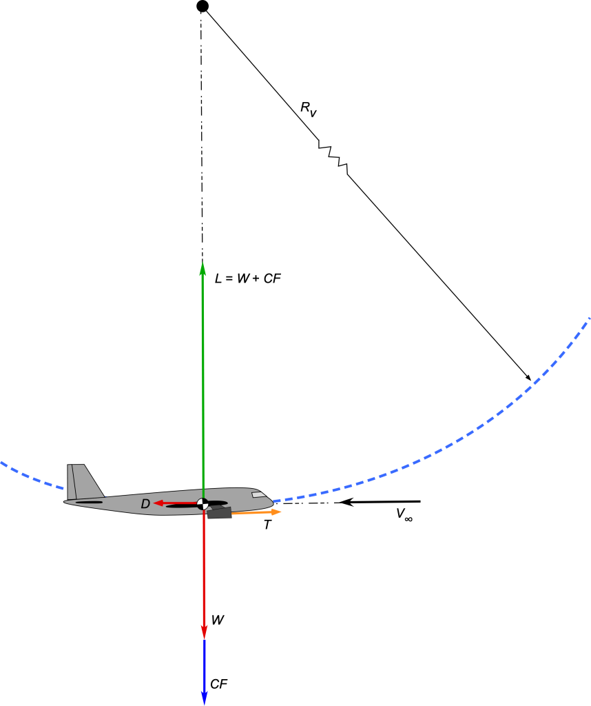
The balance of forces on an airplane at the bottom of a pull-up flight maneuver following a circular flight path in a vertical plane.

Vertical equilibrium, in this case, requires that

(20) $\begin{equation*} L - W = \left( \frac{W}{g} \right) \frac{V_{\infty}^2}{R_v} \end{equation*}$

Therefore, the lift required from the wing at the bottom of the pull-up is

(21) $\begin{equation*} L = \left( \frac{W}{g} \right) \frac{V_{\infty}^2}{R_v} + W = \left( 1 + \frac{V_{\infty}^2}{g \, R_v} \right) W = n \, W \end{equation*}$

i.e., the lift on the airplane must be greater than its weight, where the load factor $n$ is

(22) $\begin{equation*} n = \left( 1 + \frac{V_{\infty}^2}{g \, R_v} \right) \end{equation*}$

The excess lift is related to the load factor $n$ such that $L = nW$ , i.e., the number of effective $g$ loadings. So, it can be seen that for a given radius of the flight path in a pull-up, the load factor increases with the square of the airspeed. For a given airspeed, the load factor is inversely proportional to the radius, i.e., a faster and/or tighter flight path will produce a higher load factor. The radius of curvature $R_v$ of the flight path, in this case, will be

(23) $\begin{equation*} R_v = \frac{V_{\infty}^2}{g (n - 1)} \end{equation*}$

Turning Flight

Consider the forces on an airplane in a pure horizontal turn with a bank angle $\phi$ and at a constant airspeed $V_{\infty}$ , as shown in the figure below. To perform a turn, the airplane must be banked at an angle $\phi$ such that a component of the wing lift creates the necessary inward force to create the inward centripetal acceleration and so balance the outward centrifugal force, i.e., the inertial effects of the centripetal acceleration. In proceeding, it is again possible to assume that $\epsilon = 0$ .

The balance of forces on an airplane in a horizontal (no climb or descent) banked turn at a constant airspeed.

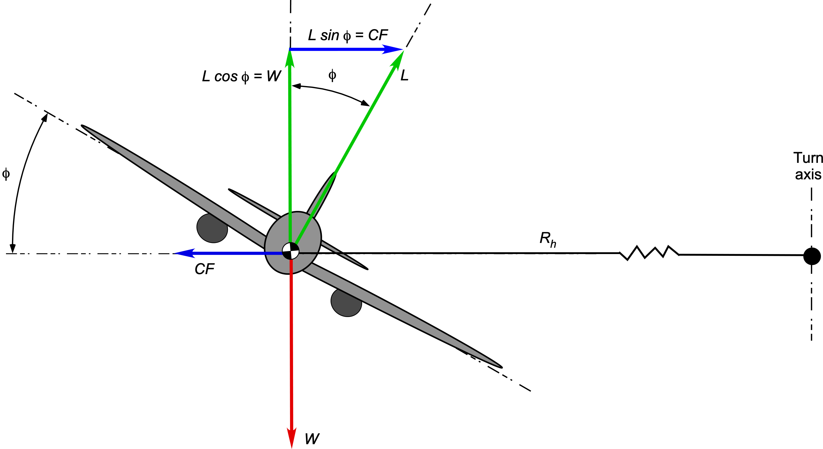
Vertical equilibrium requires that

(24) $\begin{equation*} L \cos \phi = W \end{equation*}$

Horizontal equilibrium requires that the inward component of the lift provide the centripetal acceleration, i.e.,

(25) $\begin{equation*} L \sin \phi = \left(\frac{W}{g} \right) \frac{V_{\infty}^2}{R_h} \end{equation*}$

where $R_h$ , in this case, is the radius of curvature of the horizontal turn.

It is apparent then that to perform a turn, the lift on the wing of the airplane must be greater than its weight, i.e., $L > W$ , to create the necessary aerodynamic force not only to balance the weight of the airplane but also to produce the inward radial force to create the needed centripetal acceleration to execute a turn. Solving for the lift required gives

(26) $\begin{equation*} L = \frac{W}{\cos \phi} \end{equation*}$

and the corresponding load factor is

(27) $\begin{equation*} n = \frac{W }{W \cos \phi} = \frac{1}{\cos \phi} = \sec \phi \end{equation*}$

This result shows that the load factor must increase with the inverse of the cosine of the bank angle, as shown in the figure below. For example, a 60 $^{\circ}$ banked turn will correspond to a load factor of two.

Variation of the load factor in a horizontal banked turn.

The corresponding radius of curvature of the flight path can be solved using

(28) $\begin{equation*} R_h = \frac{V_{\infty}^2}{g \sqrt{n^2 -1}} \end{equation*}$

and the rate of turn (angular velocity) in the turn is given by

(29) $\begin{equation*} \omega = \frac{d\gamma}{dt} = \frac{g \sqrt{n^2 -1}}{V_{\infty}} \end{equation*}$

Check Your Understanding #2 – Steady banked turn maneuver

Consider a fighter airplane of mass $M$ = 20,000 kg in a steady banked turn with angle $\phi$ = 65 degrees at a constant altitude.

Find the total lift needed on the wing and the corresponding load factor $n$ .
Determine an expression for the centripetal force needed to execute the turn in terms of airspeed and radius of turn.
If the airspeed is 250 knots, what will be the radius of the turn?
If the maximum allowable load factor on the airplane is $n = 7$ , what will be the corresponding maximum permissible bank angle and new turn radius at this airspeed?

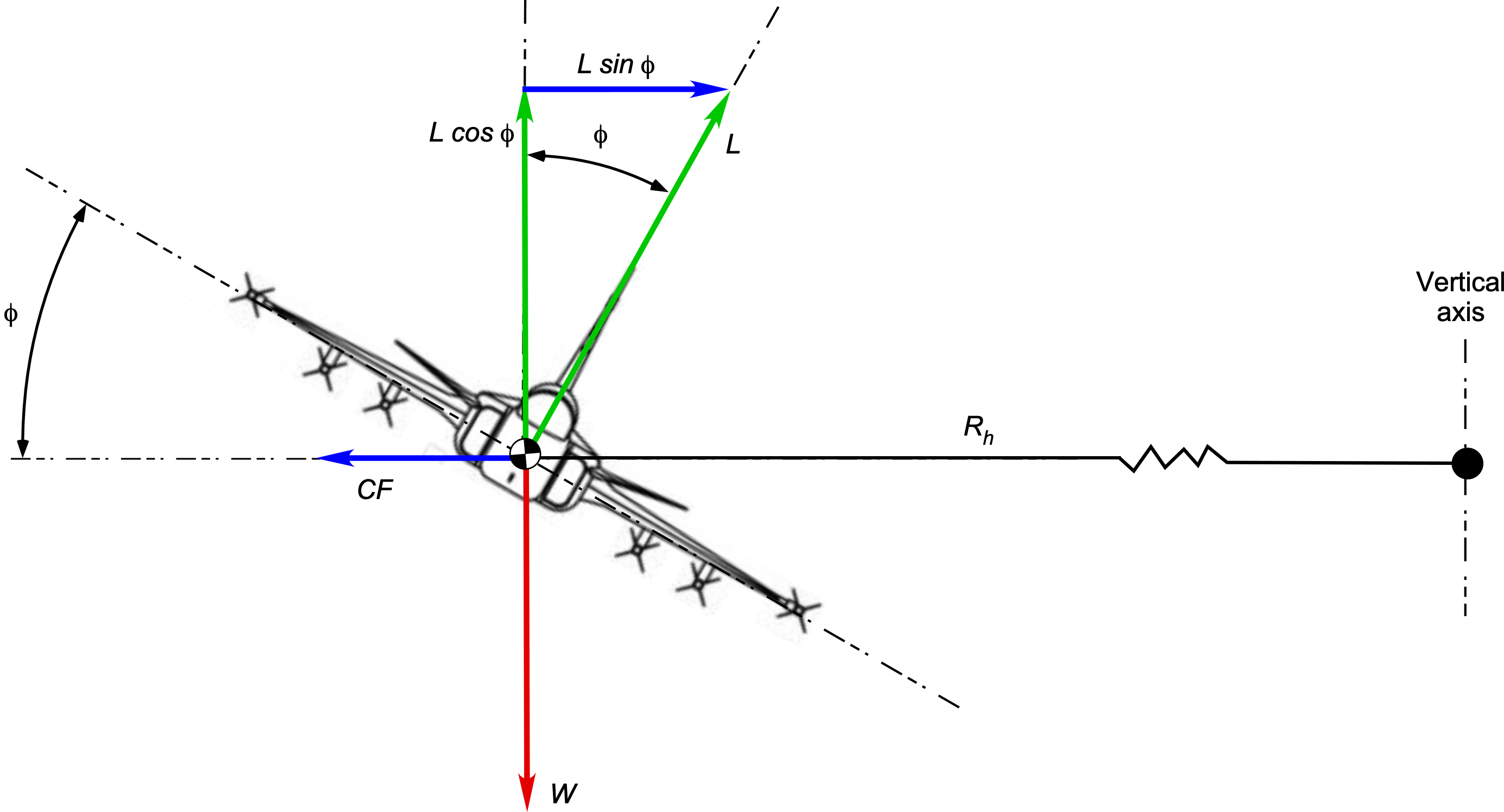
Show solution/hide solution.

1. The total lift needed on the wing will be

$L = \frac{W}{\cos \phi} = \frac{Mg}{\cos \phi} = \frac{20,000 \times 9.81}{\cos 65^{\circ}} = 464.25~\mbox{kN}$

The corresponding load factor is

$n = \frac{1}{\cos 65^{\circ}} = 2.37$

2. Concerning the figure above, the equation for the inward centripetal force $CF$ to produce this level turn is

$CF= L \sin \phi = \frac{M V_{\infty}^2}{R_h}$

where $R_h$ is the (horizontal) radius of the turn.

3. An airspeed of 250 kts is equal to 128.6 m/s, so rearranging the previous equation gives the radius of the turn as

$R_h = \frac{M V_{\infty}^2}{\sin \phi \ L} = \frac{20,000 \times 128.6^2}{\sin 65^{\circ} \times 464,249} = 786.2~\mbox{m}$

4. We are given that $n_{\rm max}$ = 7, so

$\phi_{\rm max} = \cos^{-1} \left( \frac{1}{n_{\rm max}} \right) = \cos^{-1} \left( \frac{1}{7.0} \right) = 81.8^{\circ}$

and the maximum lift on the wing will be

$L_{\rm max} = \frac{Mg}{\cos \phi_{\rm max}} = \frac{20,000 \times 9.81}{\cos 81.8^{\circ}} = 1.376\times 10^6~\mbox{N}$

The radius of the turn in this condition is

$R_h = \frac{M V_{\infty}^2}{\sin \phi_{\rm max} \ L} = \frac{20,000 \times 128.6^2}{\sin 81.8^{\circ} \times 1.376\times 10^6} = 242.9~\mbox{m}$

which is a very tight turn.

Summary of the Equations of Motion

In summary, the following general equations apply to the motion of an airplane:

(30) $\begin{eqnarray*} \mbox{$\parallel$ to flight path:} \quad && \hspace*{-7mm} \left(\frac{W}{g}\right) \frac{d V_{\infty}}{dt} = T \cos \epsilon - D - W \sin \gamma \\[12pt] \mbox{$\perp$ to flight path:} \quad && \hspace*{-7mm} \left(\frac{W}{g}\right) \frac{V_{\infty}^2}{R_v} = L \cos \phi + T \sin \epsilon \cos \phi - W \cos \gamma \\[12pt] \mbox{Horizontal plane:} \quad && \hspace*{-7mm} \left(\frac{W}{g}\right) \frac{V_{\infty}^2}{R_h} = L \sin \phi + T \sin \epsilon \sin \phi \end{eqnarray*}$

where $R_v$ = the radius of curvature of the flight path in a vertical plane, and $R_h$ = the radius of curvature of the flight path in a horizontal plane.

If the wings are level, i.e., $\phi = 0$ , then for flight in a vertical plane

(31) $\begin{eqnarray*} \mbox{$\parallel$ to flight path:} \quad && \hspace*{-7mm} \left(\frac{W}{g}\right) \frac{d V_{\infty}}{dt} = T \cos \epsilon - D - W \sin \gamma \\[12pt] \mbox{$\perp$ to flight path:} \quad && \hspace*{-7mm} \left(\frac{W}{g}\right) \frac{V_{\infty}^2}{R_v} = L + T \sin \epsilon - W \cos \gamma \end{eqnarray*}$

In many cases, the line of action of the thrust vector relative to the flight path is small, so it is reasonable to assume that $\epsilon = 0$ in the forgoing equations, i.e.,

(32) $\begin{eqnarray*} \mbox{$\parallel$ to flight path:} \quad && \hspace*{-7mm} \left(\frac{W}{g}\right) \frac{d V_{\infty}}{dt} = T - D - W \sin \theta \\[10pt] \mbox{$\perp$ to flight path:} \quad && \hspace*{-7mm} \left(\frac{W}{g}\right) \frac{V_{\infty}^2}{R_v} = L - W \cos \gamma \\[10pt] \mbox{Horizontal plane:} \quad && \hspace*{-7mm} \left(\frac{W}{g}\right) \frac{V_{\infty}^2}{R_h} = L \sin \phi \end{eqnarray*}$

Remember that in accelerated flight, the lift will not equal the airplane’s weight because the wing must create whatever lift value is needed to produce the accelerations to follow the required flight path. The resulting lift force may be greater or less than the airplane’s weight so that the load factor can be positive or negative during flight.

Under conditions where the airplane is in a steady climb with no accelerations parallel or perpendicular to the flight path, then

(33) $\begin{equation*} T - D = W \sin \gamma \end{equation*}$

and

(34) $\begin{equation*} L = W \cos \gamma \end{equation*}$

Finally, the simplest conditions are straight and level, unaccelerated flight where

(35) $\begin{equation*} T - D = 0 \quad \mbox{or} \quad T = D \end{equation*}$

and

(36) $\begin{equation*} L - W = 0 \quad \mbox{or} \quad L = W \end{equation*}$

Limiting Airspeeds & Load Factors

An airplane (or the pilot and crew) cannot withstand infinite load factors, and the airplane will be either aerodynamically or structurally limited, or both. An airspeed/load factor diagram (a so-called $V$ – $n$ diagram) is one form of operating envelope for an airplane. This diagram maps out the conditions for flight without the airplane stalling or exceeding its structural strength limits.

The figure below shows a representative $V$ – $n$ diagram for an airplane as a function of its airspeed (flight Mach number may also be used). The green area is the normal flight envelope, with the orange and red zones denoting structural overload conditions.

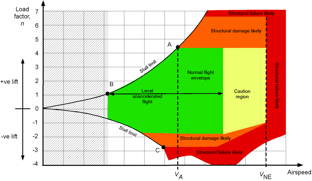Representative $V$ – $n$ diagram in terms of load factor versus airspeed.

Notice that the “stall limit” traces out one corner of the operating envelope, which is the load factor that can be attained in normal (upright flight) before the wing stalls, denoted by the region between points A and B. Point B corresponds to a level flight stall, and Point B is an accelerated stall with a limiting load factor. The other stall limit is the corresponding maximum attainable load factor before the wing stalls when the airplane is inverted, denoted by Point C; obviously, not all airplanes will be capable of inverted flight.

There is an airspeed called the “corner” airspeed, where the airplane will operate at the edge of the stall and pull the maximum load factor. This condition is identified as point A and is called the maximum maneuvering airspeed, called $V_A$ . In very turbulent or gusty atmospheric conditions, it is essential that the airplane is not structurally overstressed and must be flown at or below $V_A$ to prevent atmospheric gusts from reaching a threshold where they may structurally overload the airframe. The maximum of “never exceed” airspeed $V_{\rm NE}$ is the airspeed where the maximum allowable aerodynamic forces are produced on the airframe.

The maximum structural attainable load factor an airplane is designed to withstand depends on the particular airplane and precisely what it is intended to do. The minimum achievable positive load factor for most airplanes (the so-called limit load) is usually 3.8. However, the FARs contain more specific requirements for different types of civil airplanes. Aerobatic and military fighter airplanes are designed to tolerate much higher load factors, often between minus ten and plus 12. To the limit load factors, 50% is added for structural design purposes (i.e., a margin of safety), which becomes known as the ultimate load. Modern aircraft with fly-by-wire flight control systems may also have “g-limiters” to prevent excessive load factors that could damage the airframe.

Physiological Effects on Pilots

Higher load factor flight maneuvers can exert significant physiological effects on pilots, particularly when flying in high-performance aerobatic or military jet fighter aircraft. High positive load factors can cause blood pooling in the lower body, leading to potential symptoms (with increasing load factor) such as blurred vision, tunnel vision, grey-out or black-out, and eventual loss of consciousness. The effects are summarized in the figure below, often referred to as a Stoll chart.^[4] The eyes are especially susceptible to the reduced oxygen content in the blood, so the gradual loss of vision indicates the physiological load factor limits for any pilot or crew. Humans can be very different regarding their load factor tolerance, so the values on the Stoll chart shown below only represent an average indicator.

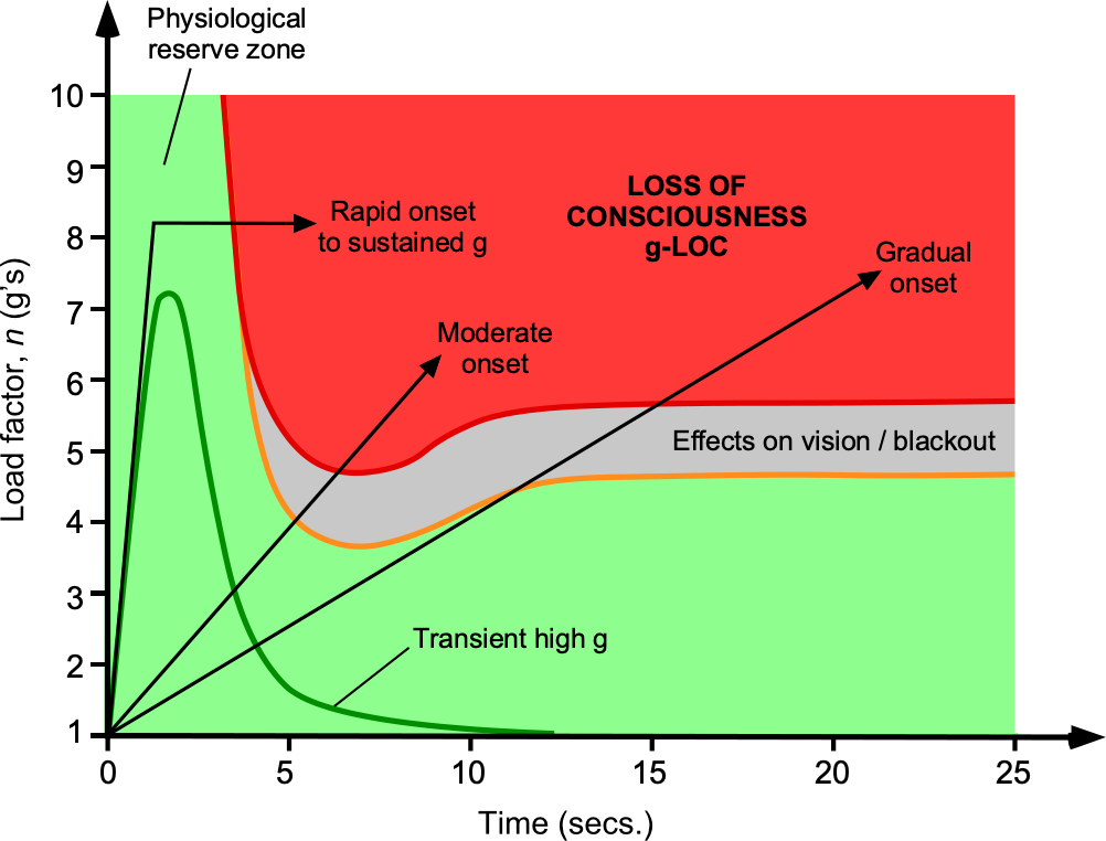
Higher load factor maneuvers, even as high as 6 or 7, can be sustained by an average human for 2 to 4 seconds without adverse effects. The blood contains a certain amount of excess oxygen, which is indicated by the physiological reserve zone on the Stoll chart. Sustained extreme load factors where $n > 6$ can cause hypoxia and the rapid onset of loss of consciousness (LOC), sometimes called “g-LOC.” The onset of LOC can also occur at lower load factors if they are applied relatively quickly, e.g., a quick pull-up maneuver with a high sustained load factor. This is a hazardous situation because it requires ten to twenty seconds for a human to recover consciousness, which is subsequently accompanied by a further period of disorientation. On regaining consciousness, pilots are usually disoriented and may still be unable to fly the airplane until the brain recovers fully from hypoxia, which may take another 20 or more seconds. Outcomes for solo pilots who suffer g-LOC during aerobatic flight are rarely good.

To counteract these symptoms, aerobatic pilots can employ anti-g straining maneuvers, which involve the tensing of specific abdominal muscles and forced breathing techniques to help maintain the blood flow to the brain. Pilots conducting extreme aerobatic flight maneuvers must undergo extensive physical training and be in top medical condition. Military fighter aircraft often use specialized equipment such as g-suits, which apply pressure to the lower body to prevent blood pooling in the legs. High negative load factors experienced during inverted flight cause blood to rush to the head, potentially leading to another type of visual impairment called red-out. Red-out can occur even at relatively low negative load factors of $n = -3$ . In addition to cardiovascular effects, high load factor aerobatic flight maneuvers impose significant musculoskeletal strain on pilots, especially in the neck and back, leading to rapid fatigue. Ergonomic considerations in cockpit design and seat construction are also essential to help mitigate the effects of high load factor “g” loading on pilots.

Summary & Closure

In the analysis of airplane performance, it has been shown how the general equations of motion for an airplane in flight can be readily derived by following the basic principles of statics and dynamics. These equations have helped expose some fundamental results for steady-level and maneuvering flight. In addition, they have set a rational basis for determining variations in the airplane’s flight performance and potential limitations. Much of the analysis of civil airplanes will be for steady-level flight, small angles of displacement, and mild maneuvers. However, for military airplanes such as fighters, their flight maneuvers may be more aggressive and include various types of aerobatics with large displacements and angular rates. In such cases, the load factors produced on the airplane may be significant, and the airplane may fly close to its aerodynamic and/or structural limits.

5-Question Self-Assessment Quickquiz

For Further Thought or Discussion

Consider an acrobatic airplane with a constant angular velocity in a roll maneuver. What factors will affect the maximum possible roll rate?
Consider a pull-down maneuver where an airplane is inverted at the top of a loop. Show how to obtain the load factor.
It is claimed that a small general aviation Cessna airplane can “out-maneuver” an F-16 fighter airplane. What does this mean, and is there any truth in this claim?
The ability to perform a banked turn will be limited by wing stall. Explain.
What factors may limit an airplane’s maximum and minimum attainable load factor? Hint: Not all of these factors may have an engineering basis.
How might the equations of motion differ for different flight regimes, e.g., subsonic, supersonic, or hypersonic?
What are the challenges in modeling and solving the airplane’s equations of motion in real-time scenarios, such as during flight simulations or control systems design?
How do the airplane’s equations of motion relate to the concepts of stability and control? How are these concepts incorporated into the design and operation of airplanes?

Other Useful Online Resources

To learn more about flight maneuvers and airplane limitations, take a look at some of these online resources:

Read the Code of Federal Regulations on the flight maneuvering envelope §25.333.
Video on flight maneuvers from ERAU.
Load factors on an airplane are explained in this video.
Zero-g flight – Parabolic flight profiles with the Airbus A300.
A video presentation giving a simplified explanation of the $V-n$ diagram
Top 8 incredible jet maneuvers ever explained!
The G-Monster is back – more 30 seconds at 9g!

Remember that when an object moves along a curved flight path, the motion is called curvilinear compared to the case where it moves in a straight line path, which is rectilinear. ↵
From the Latin word ``fugo" meaning to flee. ↵
From the Latin word ``peto'' meaning to seek. ↵
Stoll, A. M., "Human Tolerance to Positive g as Determined by Physiological Endpoints," Aviation Medicine, 1956, 27:356–367. ↵

License

Icon for the Creative Commons Attribution-NonCommercial-NoDerivatives 4.0 International License

Introduction to Aerospace Flight Vehicles Copyright © 2022–2025 by J. Gordon Leishman is licensed under a Creative Commons Attribution-NonCommercial-NoDerivatives 4.0 International License, except where otherwise noted.

Digital Object Identifier (DOI)

https://doi.org/https://doi.org/10.15394/eaglepub.2022.1066.n27