20 Continuity Equation
Introduction
Having laid down the fundamental forms of the flow models used in aerodynamic analyses, the governing equations can now be formulated to describe fluid dynamic or aerodynamic flows. The approach uses the three physical conservation principles: mass, momentum, and energy. In this first case, the applicable physical principle is that mass cannot be created or destroyed. The resulting governing equation is the continuity equation. It is a general governing equation applicable to three-dimensional, unsteady flows, and it applies to all types of flows, including compressible or incompressible, viscous or inviscid, and steady or unsteady.
Learning Objectives
- Know how to derive the most general form of the continuity equation in its control volume or integral form.
- Learn how to solve simple flow problems using the continuity equation.
- See how the continuity equation can be derived from the Reynolds Transport Equation.
Continuity Equation – Integral Form
As previously discussed, the flow model is a control volume that may either be fixed in space with the fluid moving through it (the most common application), which is called an Eulerian description of the flow, or move with the fluid such that identical fluid particles are inside it, which is called a Lagrangian model. In either case, physical conservation principles must be applied to the fluid inside the control volume and any fluid crossing its boundaries.
Flow Model
Consider a fixed finite control volume  bounded by a surface of area
  , which is in an Eulerian frame of reference, as shown in the figure below. The symbol defines the area of the closed surface that bounds the control volume containing a fluid of volume
  . The control volume is abbreviated to “C.V.” and the control surface to “C.S.” All properties are allowed to vary with spatial location (i.e., with respect to
  ,
,  , and
, and  ) and in time
  so that
(1) ![\begin{eqnarray*} \varrho & = & \varrho ( x, y, z, t ) \\[6pt] \vec{V} & = & \vec{V} (x, y, z, t) \end{eqnarray*}](https://eaglepubs.erau.edu/app/uploads/quicklatex/quicklatex.com-6e7fccb5ff30cdedf3daed860889b4dc_l3.svg "Rendered by QuickLaTeX.com")
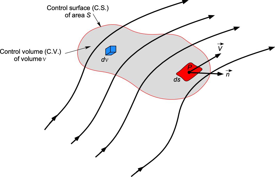
At any point on the C.S., the velocity is  , which is given in terms of the Cartesian components as
(2) 
At the same point, the unit normal vector area is  . Also, let
  be an elemental fluid volume inside the totality of the C.V.
Conservation of Mass
The fundamental principle of the conservation of mass requires that the net mass flow out of the C.V. over surface is equal to the time rate of decrease of mass inside  . Now, that physical statement must be translated into mathematics.
Following the concept of mass flow and mass flux discussed previously, the elemental mass flow across area  is
is  . Remember that by convention, always points out of the C.V., so the value of
  will be positive. Therefore, the total mass flow rate (i.e., the integral of the mass flow rate over the entire surface area) is
(3) 
which can be physically interpreted as a net outflow leaving the C.V. Notice that the double integral here means the summation over the surface , i.e., an area integral.
The small fluid mass contained within the elemental volume inside the C.V. is  . Hence, the total mass inside the C.V. is
(4) 
where the triple integral means a volume integral. So, the time rate of decrease of mass inside the C.V. is
(5) 
noting that the minus sign represents a decrease of mass, i.e., what is leaving the C.V.
Because the principle of conservation of mass requires that the net mass flow out of the C.V. be zero, then Eq. 3 must equal Eq. 5, i.e.,
(6) 
(7) ![\begin{equation*} \boxed{\underbrace{\frac{\partial}{\partial t}\oiiint_{\cal{V}} \varrho \, d {\cal{V}}}_{\begin{tabular}{c} \scriptsize Time rate of \\[-3pt] \scriptsize change of mass \\[-3pt] \scriptsize inside C.V. \end{tabular}} + \underbrace{ \oiint_S \varrho \, \vec{V} \bigcdot d\vec{S}}_{\begin{tabular}{c} \scriptsize Net mass \\[-3pt] \scriptsize flow rate \\[-3pt] \scriptsize out of C.V. \end{tabular}} = 0}^{~*} \end{equation*}](https://eaglepubs.erau.edu/app/uploads/quicklatex/quicklatex.com-06e9455be86c6a0b8fe72b1a422e45a1_l3.svg "Rendered by QuickLaTeX.com")
The latter equation in Eq. 7 is called the continuity equation for a fluid flow, in this case, in the integral or control volume form. It is a “star” equation because it is the most general form of the governing equation, i.e., it is valid for three-dimensional, unsteady flows. It applies to all types of flows, including compressible and incompressible, as well as viscous and inviscid. Additionally, it can be used to relate aerodynamic phenomena over a finite region of the flow, such as the properties of the flow as it enters and exits the specified control volume. The unknowns in the equation include the flow velocities and the flow density.
Simplifications of the Continuity Equation
Various reductions or simplifications of the continuity equation can be used to solve practical problems, and these forms also allow commensurate simplifications in the overall mathematics. For example, for a steady flow, nothing changes with respect to time, i.e.,  . This simplification means that the continuity equation reduces to
(8) 
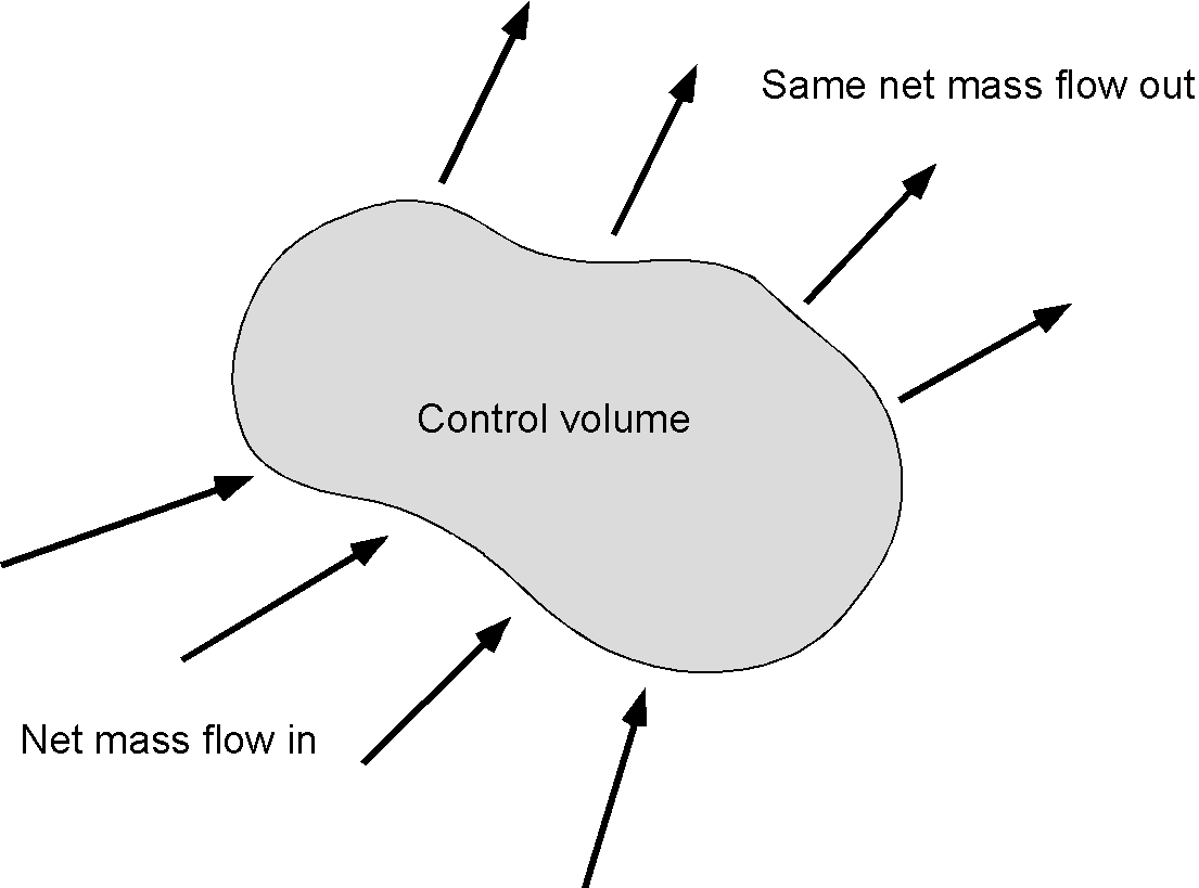
In other words, the mass flow that enters the control volume per unit of time also leaves the control volume simultaneously, i.e., no mass accumulates within the control volume. If this assumption can be justified, eliminating time dependencies in aerodynamic problems is a significant and worthwhile simplification in most forms of practical analysis.
Proceeding further by assuming that the flow is a steady single stream system and one-dimensional, e.g., a uniformly axisymmetric flow, then the reduced form of the continuity equation is
(9) 
where  is the unit vector area, which is positive when it points out of the C.V., as shown in the figure below. A much easier way to express this one-dimensional result for the continuity equation is in scalar form, such that
(10) 
which is a statement that the summation of the mass flow rates through the C.V. is constant for a steady flow.
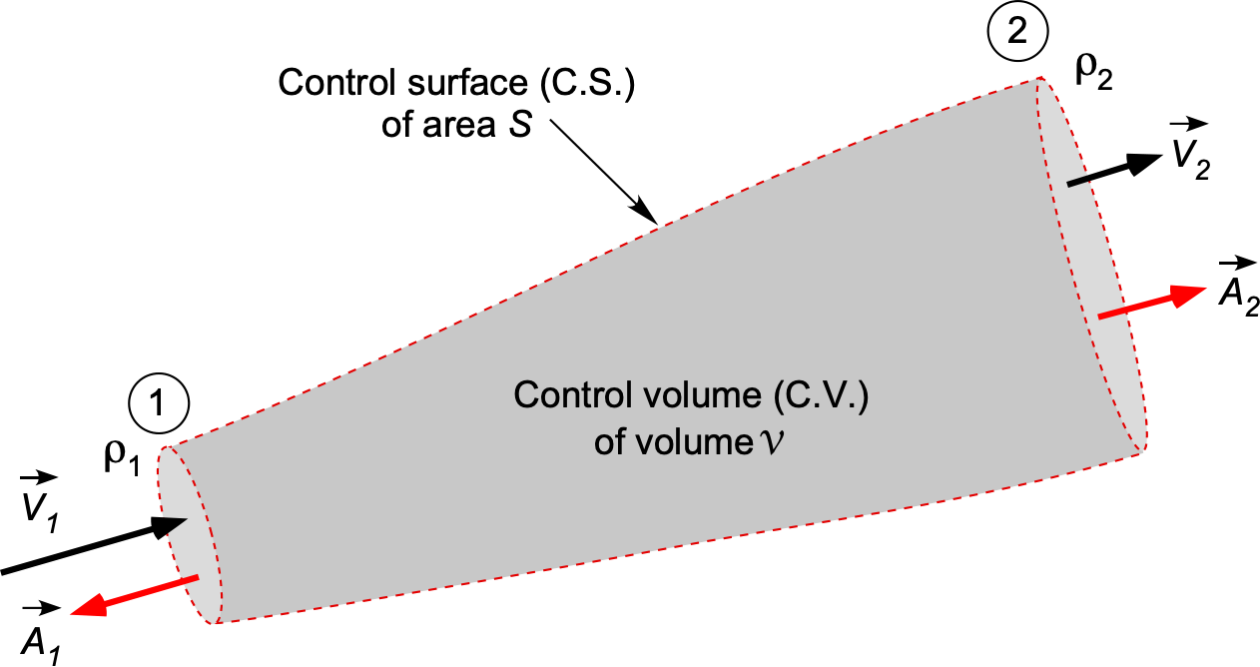
For the situation of a single stream inlet and outlet, then
(11) 
noting the sign on the first term because  is in the opposite direction to
  . This result can also be written in scalar form in terms of magnitudes as
(12) 
or
(13) 
which is just a statement that  =
=  , i.e., mass flow is conserved.
If the flow is incompressible, i.e.,  = constant, then the continuity equation becomes
(14) 
which leads to a further simplification because of the elimination of as an unknown. Therefore, only the flow velocities need to be related, i.e.,
(15) 
where  is the volume flow rate. In this case, then
(16) 
or
(17) 
which means that  =
=  , i.e., volume flow is conserved.
Finally, consider a reduction to a steady (but compressible), uniform, one-dimensional flow in the direction. In this case,  and so
(18) 
or
(19) 
Notice that the areas  and
and  become areas per unit length, i.e.,
  and
and  , respectively.
Flow Through a Converging/Diverging Duct
Consider the steady, uniform flow through a converging/diverging duct with a circular cross-section with inlet area and outlet area , as shown in the figure below. This is a classic problem when learning fluid dynamics. The two sectional regions are known, such as by measurement. If the flow is assumed to be steady and uniformly axisymmetric (i.e., one-dimensional), then determine the relevant form of the continuity equation to relate the flow conditions at the outlet to those at the inlet.
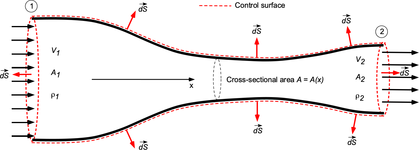
The first step in the solution is to define a coordinate system and the control surface or volume over which the principle of conservation of mass applies. In this case, the decision on the C.S. and C.V. is relatively easy, as the duct bounds the flow. There can be no mass flow over the duct walls, which is a natural consequence regardless of the duct’s shape.
The flow is steady, so , and no further justification is needed in this case. However, nothing is mentioned about whether the flow is compressible or incompressible. Because air is a gas, it must be assumed that the flow is compressible and that density must be retained as a variable. Furthermore, suppose the flow is uniformly axisymmetric. In that case, the flow velocity changes only in one direction, i.e., in the direction, based on the adopted coordinate system, which is another significant simplification in solving this problem.
In light of the preceding assumptions, therefore, in this case, then
(20) 
where the latter term is zero because there is no mass flow over the walls, i.e.,
(21) 
The mass flow coming into the C.V. through the left-hand side (face 1) is
(22) 
the one-dimensional assumption being used and the minus sign on the first term indicating that the flow is in the opposite direction to . Similarly, the flow coming out of the right-hand side (face 2) is then
(23) 
which is positive in this case because the flow is now in the direction of . Therefore, because the flow is steady, the principle of conservation of mass states that the net mass flow is zero, so what mass flow comes into the C.V. per unit time must equal the net mass flow out of the C.V. per unit time, i.e.,
(24) 
or simply that
(25) 
Rearranging the latter equation gives the outlet conditions
(26) 
i.e., the mass fluxes are related by the area ratio  . If the flow was further assumed to be incompressible, then = constant, and so
(27) 
Finally, this latter result must be examined to see if it reconciles expectations and makes sense. Engineers develop the habit of asking such questions in practical problem-solving, i.e., based on the final equation(s), do the results make physical sense?
For example, if the outlet area were to be smaller than the inlet area (i.e.,  ), then the expectation is that the flow velocity will increase as it flows into and out of the C.V., which it does according to the equations because
  . Notice that while this particular problem may appear easy, and indeed it is in this case, it provides an excellent example of how the conservation laws, in the integral form, can be applied to a fluid dynamics or aerodynamics problem.
Check Your Understanding #1 – Calculating flow velocities in a converging duct
Consider the steady flow of a particular gas through a horizontal, converging pipe with an inlet diameter  of 0.22 m and an outlet diameter
  of 0.16 m. The density of the gas is known to change from
  kg/m
kg/m at the inlet to
  kg/m at the outlet. If the inlet flow velocity of the gas
  is 5.1 m/s, what is its exit velocity
  ? Assume one-dimensional flow.
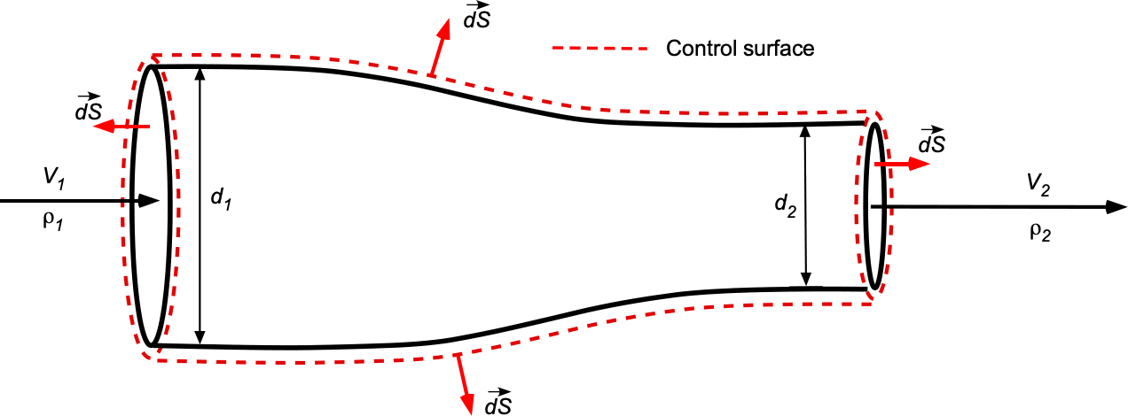
Show solution/hide solution.
The general form of the continuity equation is
![\[ \frac{\partial}{\partial t}\oiiint_{{\cal{V}}} \varrho \, d{\cal{V}} + \oiint_S \varrho \, \vec{V} \bigcdot d\vec{S} = 0 \]](https://eaglepubs.erau.edu/app/uploads/quicklatex/quicklatex.com-b25de9878de50386c16c3832b93c4307_l3.svg "Rendered by QuickLaTeX.com")
In this case, for steady, one-dimensional flow, then
(28) 
or
![\[ \overbigdot{m} = \mbox{constant} = \varrho_1 V_1 A_1 = \varrho_2 V_2 A_2 \]](https://eaglepubs.erau.edu/app/uploads/quicklatex/quicklatex.com-758fee81423c3ba890ef2b2c6ddd72dc_l3.svg "Rendered by QuickLaTeX.com")
where the density must be retained as a variable. In terms of diameters, then
![\[ \varrho_1 V_1 d_1^2 = \varrho_2 V_2 d_2^2 \]](https://eaglepubs.erau.edu/app/uploads/quicklatex/quicklatex.com-7b3937745942aae3e3f284885d536a22_l3.svg "Rendered by QuickLaTeX.com")
Solving for gives
![\[ V_2 = \frac{\varrho_1 V_1 d_1^2}{\varrho_2 d_2^2} \]](https://eaglepubs.erau.edu/app/uploads/quicklatex/quicklatex.com-506a519b78ff00875a72971352473b7a_l3.svg "Rendered by QuickLaTeX.com")
Substituting the numerical values gives
![\[ V_2 = \frac{0.91 \times 5.1 \times 0.22^2}{0.83 \times 0.16^2} = 10.57~\mbox{m s$^{-1}$} \]](https://eaglepubs.erau.edu/app/uploads/quicklatex/quicklatex.com-7dc0ec8d0543ca4f0a42c753564ba047_l3.svg "Rendered by QuickLaTeX.com")
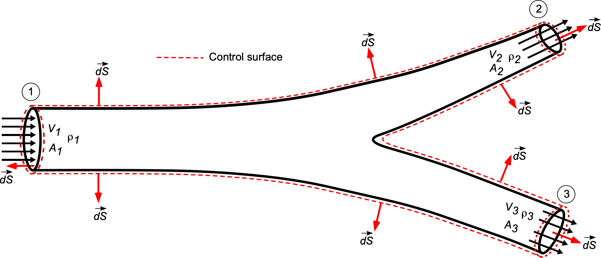
Flow Through a Branched Pipe
Consider the flow of fluid through a branch circuit of a pipe, as shown below. The objective, again, is to use the principles of the conservation of mass to determine a relationship between the flow properties and the inlet and outlet conditions. The inlet and outlet areas of the pipe are assumed to be known. Remember that the first step in the analysis is to sketch the C.V. and the C.S. and annotate them appropriately. It will be assumed that the fluid is incompressible, i.e.,  constant, steady, and one-dimensional; the one-dimensional assumption is that the flow velocities are constant over every cross-section.
The governing equation for continuity of flow, in this case, becomes
(29) 
where the mass flow over the solid walls would be zero, i.e.,
(30) 
If the flow velocities are constant over their respective areas (the one-dimensional assumption), then
(31) 
And if the density is constant (which it is for a liquid), then
(32) 
noting the negative sign on the first term and its significance. Another way of looking at this latter result for the branch flow is to write it as
(33) 
where is the volume flow rate. Of course, if there were no third exit, then the problem could be reduced to the one previously considered, and
(34) 
In general, considering the flow out of the junction as positive and the flow into the junction as negative, then for steady flow at any junction, the algebraic sum of all the mass flows must be zero, i.e.,
(35) 
For an incompressible flow, i.e., a liquid, then volume is also conserved, i.e.,
(36) 
Check Your Understanding #2 – Converging flows into a junction
Two pipes of diameters and converge to form a single pipe of diameter  . If a liquid flows with a velocity of and in the two pipes, respectively, what will be the flow velocity
  in the third pipe? Assume steady, one-dimensional, incompressible flow with no losses.
Show solution/hide solution.
In this case, two pipes merge to form a single pipe. Conserving mass and using average flow properties, then
![\[ \overbigdot{m} = \mbox{constant} = \varrho_1 V_1 A_1 + \varrho_2 V_2 A_2 = \varrho_3 V_3 A_3 \]](https://eaglepubs.erau.edu/app/uploads/quicklatex/quicklatex.com-cd23ed298199576f90397c401c3e8787_l3.svg "Rendered by QuickLaTeX.com")
If the fluid is a liquid then the assumption that =  =
=  =
=  = constant is justified so
![\[ Q = \mbox{constant} = V_1 A_1 + V_2 A_2 = V_3 A_3 \]](https://eaglepubs.erau.edu/app/uploads/quicklatex/quicklatex.com-bdbc37904a67d1efc5f6bce5443fe45e_l3.svg "Rendered by QuickLaTeX.com")
Therefore, the flow velocity in the third pipe is
![\[ V_3 = \frac{V_1 A_1 + V_2 A_2}{A_3} = \frac{V_1 (\pi \, d_1^2/4) + V_2 (\pi \, d_2^2/4)}{ (\pi \, d^2/4)} = \frac{V_1 \, d_1^2 + V_2 \, d_2^2}{d^2} \]](https://eaglepubs.erau.edu/app/uploads/quicklatex/quicklatex.com-9dca0b6a19b46b74c1a2ff93ecd19317_l3.svg "Rendered by QuickLaTeX.com")
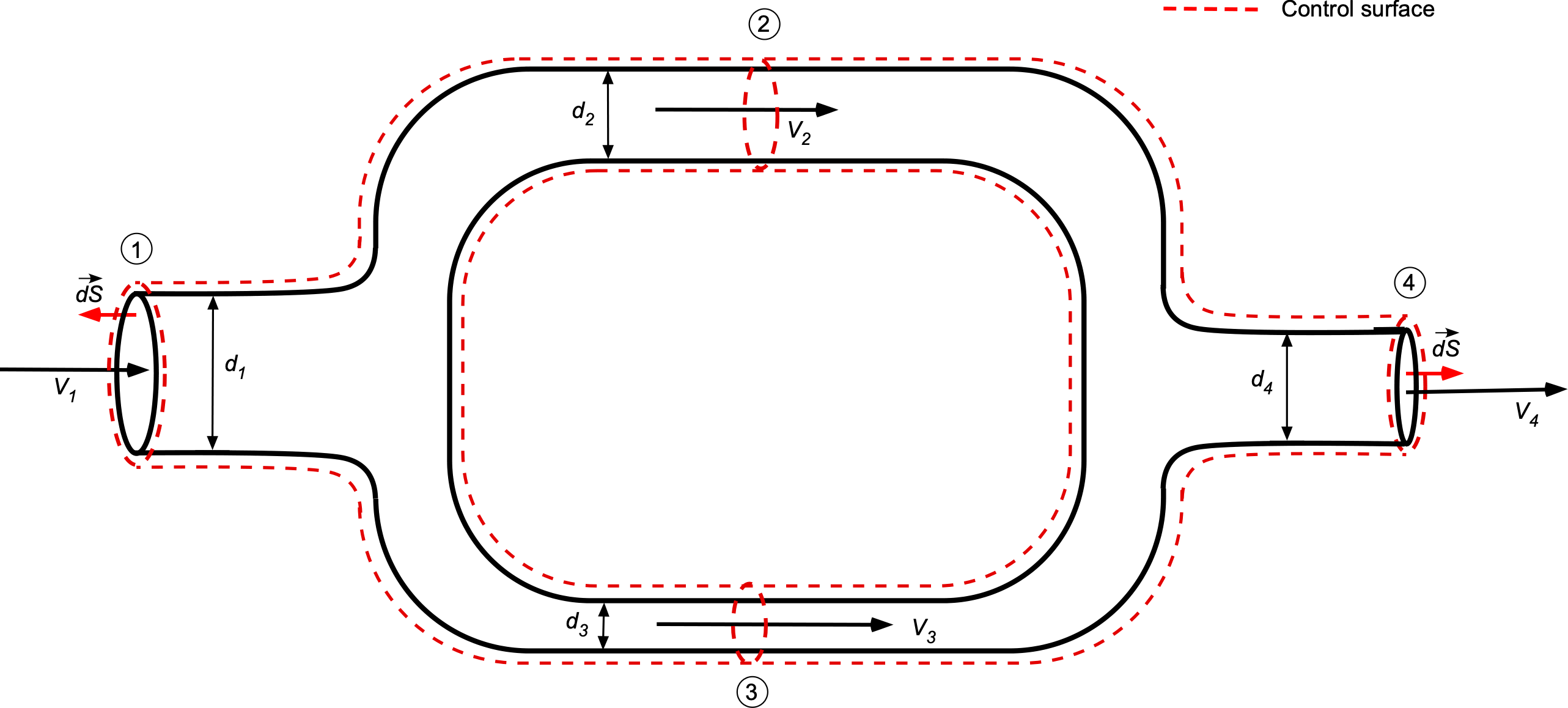
Flow Through Parallel Pipes
Consider the flow of fluid that splits through a branch circuit with parallel circular pipes, as shown in the figure below, and then joins together again. The flow enters at 1 and leaves at 4. The two branches, 2 and 3, could have different cross-sectional areas. Again, it will be assumed that the fluid is incompressible, i.e., constant, steady, and one-dimensional; recall that the one-dimensional assumption is that the flow velocities are constant over every cross-section.
The governing continuity equation is
(37) 
Notice also that for the two branches that
(38) 
If the flow velocities are constant over their respective areas (i.e., the one-dimensional assumption), then
(39) 
If the density is constant, then
(40) 
or
(41) 
where is the volume flow rate. Notice that for the branches, then
(42) 
Check Your Understanding #3 – Flows through parallel pipes
Water flows through a central pipe, which splits into two parallel pipes and then rejoins into a single pipe downstream. The main pipe has a diameter of 10 cm, one parallel pipe has a diameter of 6 cm, and the other has a diameter of 4 cm. If the velocity of the water in the main pipe before the split is 2.0 m/s, find the velocities in each parallel pipe. Assume steady, one-dimensional, incompressible flow with no losses.
Show solution/hide solution.
For the main pipe, the area is
![\[ A_1 = \pi \left(\frac{d_1}{2}\right)^2 = \pi \left(\frac{10}{2}\right)^2 = 25\pi \, \mbox{cm}^2 \]](https://eaglepubs.erau.edu/app/uploads/quicklatex/quicklatex.com-8c46a2e6374c88519c97a214cd571920_l3.svg "Rendered by QuickLaTeX.com")
For the first parallel pipe (6 cm diameter), the area is
![\[ A_2 = \pi \left(\frac{d_2}{2}\right)^2 = \pi \left(\frac{6}{2}\right)^2 = 9\pi \, \text{cm}^2 \]](https://eaglepubs.erau.edu/app/uploads/quicklatex/quicklatex.com-06097b9b70c38385df870636cb99e361_l3.svg "Rendered by QuickLaTeX.com")
and for the second parallel pipe (4 cm diameter)
![\[ A_3 = \left(\frac{d_3}{2}\right)^2 = \pi \left(\frac{4}{2}\right)^2 = 4\pi \, \text{cm}^2 \]](https://eaglepubs.erau.edu/app/uploads/quicklatex/quicklatex.com-ef617eb2f00df02091e6f51042f87d0e_l3.svg "Rendered by QuickLaTeX.com")
The continuity equation for incompressible flow states that the flow rate in the main pipe must equal the combined flow rate in the parallel pipes, i.e.,
![\[ Q = A_1 V_1 = A_2 V_2 + A_3 V_3 \]](https://eaglepubs.erau.edu/app/uploads/quicklatex/quicklatex.com-cf2157818c1aacb6319288e597977ed4_l3.svg "Rendered by QuickLaTeX.com")
Substituting the numerical values gives
![\[ 25\pi \times 2 = 9\pi \times V_2 + 4\pi \times V_3 \]](https://eaglepubs.erau.edu/app/uploads/quicklatex/quicklatex.com-b8445f914b9d00e4789a226f76a0f8f0_l3.svg "Rendered by QuickLaTeX.com")
leading to
![\[ 50 = 9V_2 + 4V_3 \]](https://eaglepubs.erau.edu/app/uploads/quicklatex/quicklatex.com-67fad8565ad2dde9979b9ed51c1d22d9_l3.svg "Rendered by QuickLaTeX.com")
It will be apparent that and can only be solved uniquely with additional information or assumptions. One reasonable assumption is to assume that the flow is split proportionally based on the cross-sectional areas, which means the velocity in each pipe is inversely proportional to its cross-sectional area, i.e.,
![\[ \frac{V_2}{V_3} = \frac{A_3}{A_2} = \frac{4}{9} \]](https://eaglepubs.erau.edu/app/uploads/quicklatex/quicklatex.com-39090ced239a0b82317bafbfec04be7d_l3.svg "Rendered by QuickLaTeX.com")
Proceeding with this assumption gives
![\[ V_2 = \frac{4}{9} V_3 \]](https://eaglepubs.erau.edu/app/uploads/quicklatex/quicklatex.com-e26930d5a785c7b7a5803b6b09ac0b4b_l3.svg "Rendered by QuickLaTeX.com")
Substituting this into the continuity equation gives
![\[ 50 = 9 \left(\frac{4}{9} V_3\right) + 4V_3 = 4V_3 + 4V_3 = 8V_3 \]](https://eaglepubs.erau.edu/app/uploads/quicklatex/quicklatex.com-31ab1f5405fd55e4156f7e0151d34efc_l3.svg "Rendered by QuickLaTeX.com")
Therefore,
![\[ V_3 = \frac{50}{8} = 6.25~\mbox{m/s} \quad \mbox{ and} \mbox V_2 = \frac{4}{9} \times 6.25 = 2.78~\mbox{m/s} \]](https://eaglepubs.erau.edu/app/uploads/quicklatex/quicklatex.com-460eb99a33eb8c34315fc77fa0a7e1f0_l3.svg "Rendered by QuickLaTeX.com")
Continuity Equation – Differential Form
To derive the continuity equation in its differential form, consider a small fluid element in the flow field defined in a Cartesian coordinate system with length dimensions  ,
,  , and
, and  , as shown in the figure below. The volume of this fluid element is
  , and so the mass of the fluid element is
(43) 
where is the fluid density at point B in three-dimensional space and time , i.e.,  .
.

The net mass flow rate through the differential element is the sum of the mass rates through each pair of opposite faces of the element. Consider first the mass flow in the direction through the left face of the element of area  , i.e.,
(44) 
where  is the velocity component of the flow in the direction. Likewise, for the right face of the element of area , then
(45) 
Therefore, the total mass flow rate through the element in the  direction is
(46) 
Similarly, for the and directions, then
(47) 
and
(48) 
where  and
and  are the velocity components in the and directions, respectively. Therefore, the total net mass flow rate out of the differential element is the sum of the net fluxes in all three directions, i.e.,
(49) 
Now, consider the time rate of change of mass inside the differential element (fixed volume), which will be
(50) 
If mass is conserved (and the volume element is fixed in space and time), then the net mass flow rate out of the fluid element is equal to the time rate of decrease of mass inside the fluid element, i.e.,
(51) 
and rearranging and simplifying gives
(52) 
Therefore, the differential form of the continuity equation (using vector notation) becomes
(53) 
where  . This is a mathematical statement in differential form, stating that mass is neither created nor destroyed.
Proceeding by noticing that expanding  using the product rule gives
(54) 
so the continuity equation now becomes
(55) 
The left-hand side contains the terms that make up the substantial derivative of , i.e.,
(56) 
so the final form of the continuity equation becomes
(57) 
As in the case of the integral form in Eq. 7, the result in Eq. 57 applies to all types of flows, e.g., compressible or incompressible, viscous or inviscid.
Simplifications to the general form of the continuity equation include steady flow, i.e.,  , and incompressible flow, i.e., = constant. If the flow is steady and incompressible, the continuity equation becomes
![\[ \nabla \bigcdot \vec{V} = 0 \]](https://eaglepubs.erau.edu/app/uploads/quicklatex/quicklatex.com-1f9d2b52eb9413b2e5e9569187de8036_l3.svg "Rendered by QuickLaTeX.com")
or in terms of the scalar components when , then
![\[ \nabla \bigcdot \vec{V} = \frac{\partial u}{\partial x} + \frac{\partial v}{\partial y} + \frac{\partial w}{\partial z} = 0 \]](https://eaglepubs.erau.edu/app/uploads/quicklatex/quicklatex.com-299d208c7a979ba1bdc401da287e8b2f_l3.svg "Rendered by QuickLaTeX.com")
Therefore, this latter equation states that to satisfy the conservation of mass, the divergence of the local velocity field must be identically zero. If it is not, then the flow would be non-physical. Notice that this condition must be satisfied regardless of whether the flow is steady or unsteady.
Check Your Understanding #4 – Physically possible flow?
Consider a steady, incompressible flow of an inviscid fluid in a two-dimensional space described by the velocity field
![\[ \vec{V} = (u, v) = (y, -x) \]](https://eaglepubs.erau.edu/app/uploads/quicklatex/quicklatex.com-8d0881d82384e476d49450c6b22d118b_l3.svg "Rendered by QuickLaTeX.com")
- Does this flow exist (physically)?
- Derive the equations of the streamlines for this velocity field.
- Sketch the streamlines and show their direction.
Show solution/hide solution.
- The differential form of the continuity equation is
![\[ \nabla \bigcdot \vec{V} = \frac{\partial u}{\partial x} + \frac{\partial v}{\partial y} \]](https://eaglepubs.erau.edu/app/uploads/quicklatex/quicklatex.com-f4400631358ccc1d2dabdb6110832d0d_l3.svg "Rendered by QuickLaTeX.com")
For
 and
and  :
:![\[ \frac{\partial u}{\partial x} = 0 \quad \mbox{and} \quad \frac{\partial v}{\partial y} = 0 \]](https://eaglepubs.erau.edu/app/uploads/quicklatex/quicklatex.com-ddd801a59c1c2b1bcacd23dee9c46db9_l3.svg "Rendered by QuickLaTeX.com")
Therefore, the continuity equation is satisfied, i.e.,
![\[ \nabla \bigcdot \vec{V} = 0 + 0 = 0 \]](https://eaglepubs.erau.edu/app/uploads/quicklatex/quicklatex.com-da28e8cb7dcd9524ffef6784ccb723e8_l3.svg "Rendered by QuickLaTeX.com")
so this IS a physically possible flow.
- The equation of the streamline in 2D is
![\[ \frac{dy}{dx} = \frac{v}{u} = \frac{-x}{y} \]](https://eaglepubs.erau.edu/app/uploads/quicklatex/quicklatex.com-e0d976aea212e32b4aebe6c86643dd2b_l3.svg "Rendered by QuickLaTeX.com")
Separating variables and integrating both sides gives
![\[ \int y \, dy + \int x \, dx = C \]](https://eaglepubs.erau.edu/app/uploads/quicklatex/quicklatex.com-099e02e2b77b9847d0a8f5b660fc6a3c_l3.svg "Rendered by QuickLaTeX.com")
The solution is
![\[ y^2 + x^2 = C \quad (C = R^2 ?) \]](https://eaglepubs.erau.edu/app/uploads/quicklatex/quicklatex.com-41149b2da0e51866dbb41a209455f20f_l3.svg "Rendered by QuickLaTeX.com")
- These are clockwise-rotating circular streamlines centered at the origin, known as a forced vortex.
Continuity Equation from the RTE
Recall that the Reynolds Transport Equation (RTE) can be expressed as
(58) ![\begin{equation*} \underbrace{\frac{D}{Dt} \oiiint_{\mathrm{sys}} \beta \, \varrho \, d\mathcal{V}}_{\begin{tabular}{c} \scriptsize Time rate of \\[-3pt] \scriptsize change of $B$ \\[-3pt] \scriptsize inside the system.\end{tabular}} = \underbrace{\frac{\partial}{\partial t} \oiiint_{\mathcal{V}} \beta \, \varrho \, d\mathcal{V}}_{\begin{tabular}{c} \scriptsize Time rate \\[-3pt] \scriptsize of change of $B$ inside\\[-3pt] \scriptsize the control volume.\end{tabular}} + \underbrace{\oiint_{S} \beta \, \varrho ( \vec{V}_{\mathrm{rel}} \bigcdot d\vec{S}) }_{\begin{tabular}{c} \scriptsize Rate at which $B$ is \\[-3pt] \scriptsize leaving through the \\[-3pt] \scriptsize control surface.\end{tabular} } \end{equation*}](https://eaglepubs.erau.edu/app/uploads/quicklatex/quicklatex.com-1e4c580a02104d494756d6558450aec5_l3.svg "Rendered by QuickLaTeX.com")
Integral Form
In the case of mass, then  , and for a fixed C.V., the mass of the system and the C.V. are the same, so
(59) 
Therefore, the RTE becomes
(60) 
or
(61) 
which will be recognized as the continuity equation in its integral form, i.e., Eq. 7.
Differential form
The differential form of the continuity equation can also be derived from the RTE. Recall that using the divergence theorem, the RTE for a fixed control volume becomes
(62) ![\begin{equation*} \oiiint_{{\cal{V}}} \bigg[ \frac{\partial (\beta \, \varrho)}{\partial t} + \beta \, \varrho \,\left( \nabla \bigcdot \vec{V} \right) \bigg] d{\cal{V}} = 0 \end{equation*}](https://eaglepubs.erau.edu/app/uploads/quicklatex/quicklatex.com-28e2f475a6c5f3056e29827261eeeec4_l3.svg "Rendered by QuickLaTeX.com")
The control volume is arbitrary, so the integrand must also be zero, and the differential form of the RTE becomes
(63) 
where, in this case, , and the mass of the system and the C.V. are the same. Therefore,
(64) 
which will be recognized as Eq. 57 given previously and will apply at every point in the flow.
Check Your Understanding #5 – Discerning a Velocity Field
Consider an incompressible, two-dimensional, steady flow field where the velocity components are given by  and
and  , where
  is a constant. 1. Show that the given velocity field satisfies the incompressible continuity equation. 2. Explain the physical significance of the given velocity components and what type of flow they represent.
Show solution/hide solution.
The incompressible continuity equation in two dimensions is
![\[ \frac{\partial u}{\partial x} + \frac{\partial v}{\partial y} = 0 \]](https://eaglepubs.erau.edu/app/uploads/quicklatex/quicklatex.com-5ff2d5048c060de8b768db7b37e08801_l3.svg "Rendered by QuickLaTeX.com")
Computing the partial derivatives gives
![\[ \frac{\partial u}{\partial x} = \frac{\partial (-2Ax)}{\partial x} = -2A \]](https://eaglepubs.erau.edu/app/uploads/quicklatex/quicklatex.com-b37226252c0e990e35fea98f2fbdd82d_l3.svg "Rendered by QuickLaTeX.com")
and
![\[ \frac{\partial v}{\partial y} = \frac{\partial (Ay)}{\partial y} = A \]](https://eaglepubs.erau.edu/app/uploads/quicklatex/quicklatex.com-6da0b529e414eb6780e58d52c7cbe0f8_l3.svg "Rendered by QuickLaTeX.com")
so that
![\[ \frac{\partial u}{\partial x} + \frac{\partial v}{\partial y} = -2A + A = -A \]](https://eaglepubs.erau.edu/app/uploads/quicklatex/quicklatex.com-2d28da70471d6753f797fcee68992e1c_l3.svg "Rendered by QuickLaTeX.com")
Because  , the given velocity field does not satisfy the incompressible continuity equation. This outcome suggests an error or violation of an assumption in the problem setup. To ensure incompressibility, we can proceed to correct the velocity field to satisfy the continuity equation. Suppose the corrected velocity components are
  and
and  , then
![\[ \frac{\partial u}{\partial x} = \frac{\partial (-Ay)}{\partial x} = 0 \]](https://eaglepubs.erau.edu/app/uploads/quicklatex/quicklatex.com-5a21ffe48690f5351f181cad0084c22c_l3.svg "Rendered by QuickLaTeX.com")
and
![\[ \frac{\partial v}{\partial y} = \frac{\partial (Ax)}{\partial y} = 0 \]](https://eaglepubs.erau.edu/app/uploads/quicklatex/quicklatex.com-816929412368ae806918c966d9e11dc9_l3.svg "Rendered by QuickLaTeX.com")
so that
![\[ \frac{\partial u}{\partial x} + \frac{\partial v}{\partial y} = 0 + 0 = 0 \]](https://eaglepubs.erau.edu/app/uploads/quicklatex/quicklatex.com-e02141908a33c6cc3821f5fccb09eb59_l3.svg "Rendered by QuickLaTeX.com")
which now satisfies the incompressible continuity equation. Notice that the corrected velocity components represent a rotational flow where implies a velocity in the direction that varies linearly with , and implies a velocity in the direction that varies linearly with . This flow type is often seen in a vortex or other rotational motion, where the fluid exhibits circular or spiral patterns around a central point.
Summary & Closure
Applying the principle of the conservation of mass to fluids results in a governing “star” equation called the continuity equation. This equation applies to all fluids, regardless of whether they are viscous or inviscid, compressible or incompressible, and whether the flow is steady or unsteady. In application, the continuity equation can be simplified from its most general form by making various assumptions that may apply to the problem of interest. However, it should be remembered that all assumptions must be justified, which in some cases may be challenging to establish a priori; therefore, caution should be exercised. The most common simplification is to write the continuity equation in one-dimensional form, i.e., in terms of fluid properties that change in only one direction. While the continuity equation can help solve certain simple classes of fluid flow problems, the solution of most real-world problems generally requires the application of conservation principles of momentum and energy to obtain the necessary information.
5-Question Self-Assessment Quickquiz
For Further Thought or Discussion
- Consider a scenario where the size of the control volume changes over time. What form of the continuity equation would be needed in this case?
- Think of some fluid flow problems where a Lagrangian flow model might be preferable to solve the problem.
- How might the continuity equation be applied to analyze blood flow in arteries and veins in the human circulatory system?
- Explain how the continuity equation could be used to design and analyze water distribution systems, such as municipal water supply networks.
- How does the continuity equation relate to streamlines in fluid flow? Provide an example to illustrate this relationship.
Additional Online Resources
- A good video on some basics of the continuity equation.
- Another video on the use of the continuity equation in fluid mechanics.
- A simple application of the conservation of mass for a fire hose.
- The Continuity Equation (Fluid Mechanics In Medicine).
- The Continuity Equation: A PDE for Mass Conservation, from Gauss’s Divergence Theorem.
- Derivation of the Continuity Equation from the University of Colorado Boulder.,
