27 Internal Flows
Introduction
Aerospace engineers are often concerned with external fluid flows, such as the flow that develops over the outside surfaces of a body, including an airfoil, wing, or a complete flight vehicle. However, internal fluid flows are also crucial in many aerospace engineering applications. An internal flow can be defined as a flow in which its downstream development is confined or altered by all of the boundary surfaces inside which it flows. Internal flows may comprise gases, such as air, and liquids. The flow of liquids is often referred to as hydraulics, a field that is studied extensively and applied in all branches of engineering.
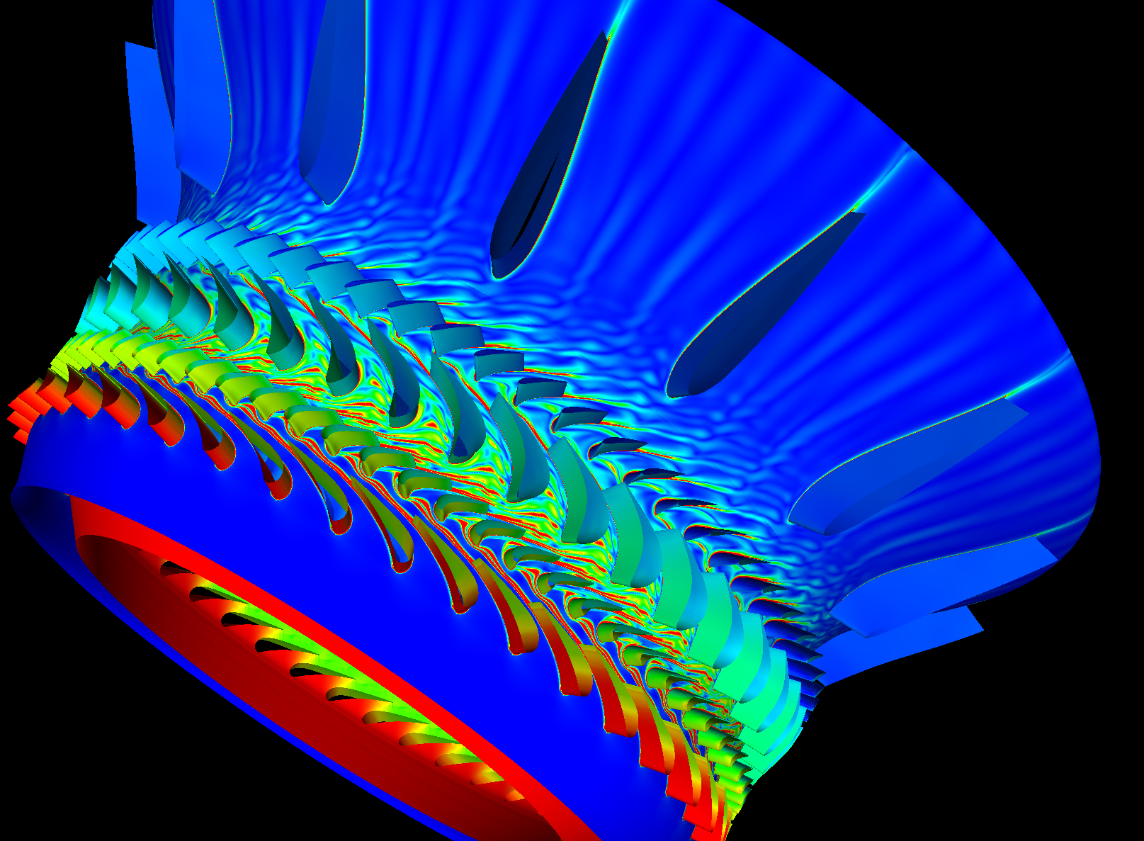
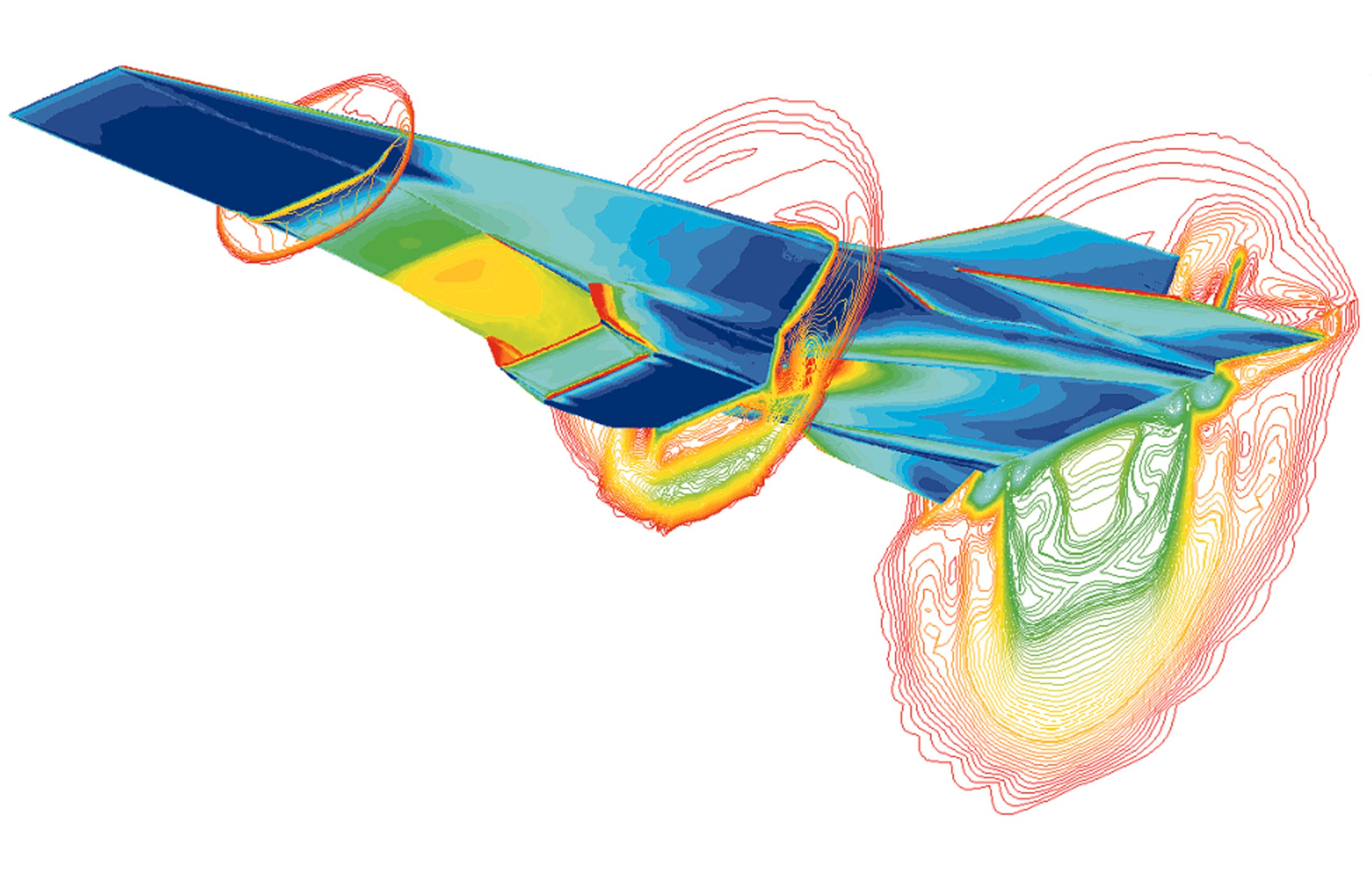
Such internal flows are encountered but are not limited to flows inside engines and combustion chambers, engine intake systems, pneumatic and hydraulic systems, fuel systems, heat exchangers and cooling systems, air conditioning systems, fire suppression systems, and wind tunnels. The figure below shows one example of an internal flow through part of a jet engine. Velocity non-uniformities from the wakes behind each blade affect the engine performance and the noise it generates.
Learning Objectives
- Appreciate the differences between external flows and internal flows, as well as understand why the action of viscous effects gives pressure losses for internal flows.
- Distinguish between the different effects caused by laminar and turbulent flows through pipes and ducts.
- Calculate the frictional losses and pressure drops associated with the flows through pipes and ducts using the Colebrook-White equation and a Moody Chart.
- Estimate the pumping power requirements to create specific mass flows and flow velocities through pipes and ducts.
- Understand the design process of producing specific flow velocities in wind tunnels and calculating power requirements.
Internal Versus External Flows
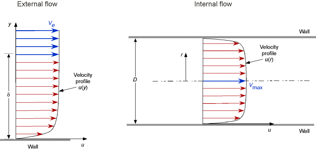
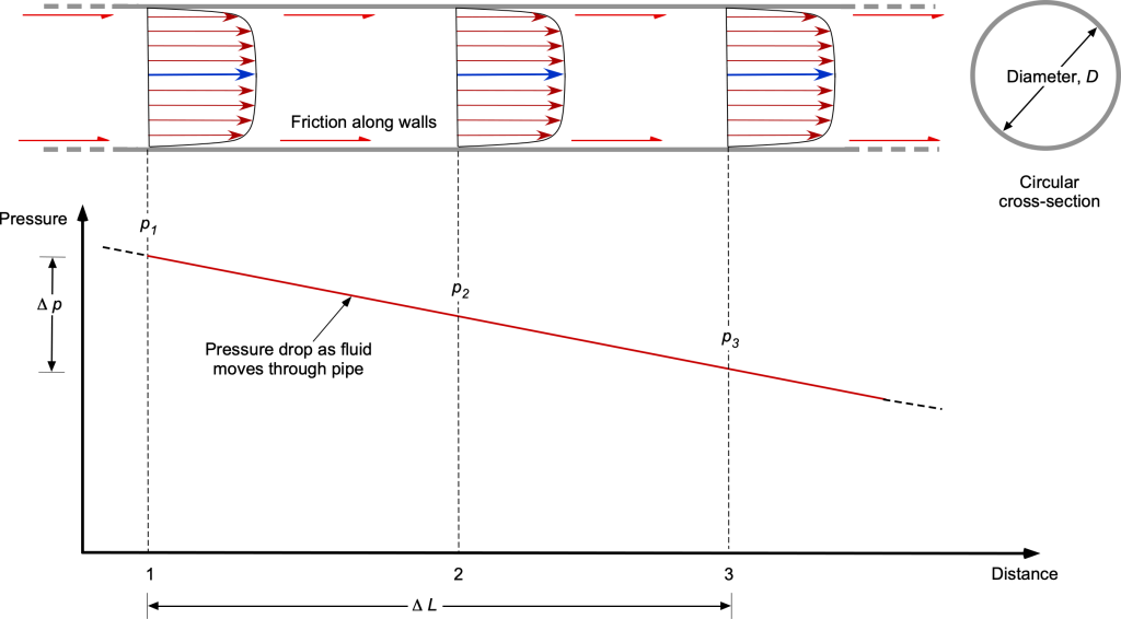
An interesting consequence of all internal flows is that the associated surface boundary layers cannot develop freely, and the flows on each inner surface merge. In this regard, the boundary layer thickness and other properties will not be the same as those of a boundary layer formed over an external surface, as illustrated in the figure below. This outcome is achieved because, for external flows, the boundaries or surfaces (often referred to as walls) introduce viscous effects into the flow that progressively diminish away from the wall. However, for internal flows, all parts of the walls of a duct, tube, or pipe constrain the flow development, so the entire cross-section of the internal flow is affected by the walls.
The foregoing behavior of the surface boundary layers is one reason why external and internal flows must be carefully distinguished; i.e., all the boundaries in an internal flow will affect each other. Because viscous losses (i.e., skin friction) are significant along all flow surfaces, for an internal flow, these effects manifest as significant pressure drops over the length of the interior surfaces where the fluid flows; the friction and the associated energy loss are irrecoverable and appear as heat. Evaluating these pressure drops is crucial for understanding internal flows and determining the engineering requirements for moving fluids through pipes and ducts.
Internal Flow Problems
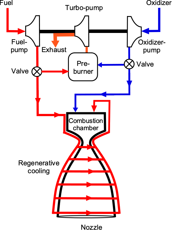
Internal fluid flow problems occur in many aerospace systems, including fuel, hydraulic, and pneumatic systems. A rocket engine, for example, as shown in the schematic below, has many internal flows that require very high mass flow rates of fuel and oxidizer. These fluids must pass through several pumps, pipes, and valves, resulting in significant pressure losses. Fuel is also pre-circulated in channels or a jacket around the exhaust nozzle to keep it cool, over which considerable pressure drops also occur. Therefore, turbopumps are needed to deliver the fuel and oxidizer to the combustion stage of the rocket engine, which usually involves the flow of cryogenic liquids at extremely high mass flow rates.
For aircraft, their hydraulic systems operate at relatively high pressures. Hence, they require high flow rates to operate the large actuators that power their landing gear, flaps, slats, flight control systems, and other components. Additionally, the hydraulic lines may extend through the structure over considerable distances, resulting in significant pressure drops. Aircraft typically have multiple hydraulic systems for redundancy in the event of failure, ensuring the systems are entirely independent. Airliners, for example, usually have three parallel hydraulic systems, each comprising multiple engine-driven pumps, electrical pumps, air-driven pumps, and hydraulic pumps.
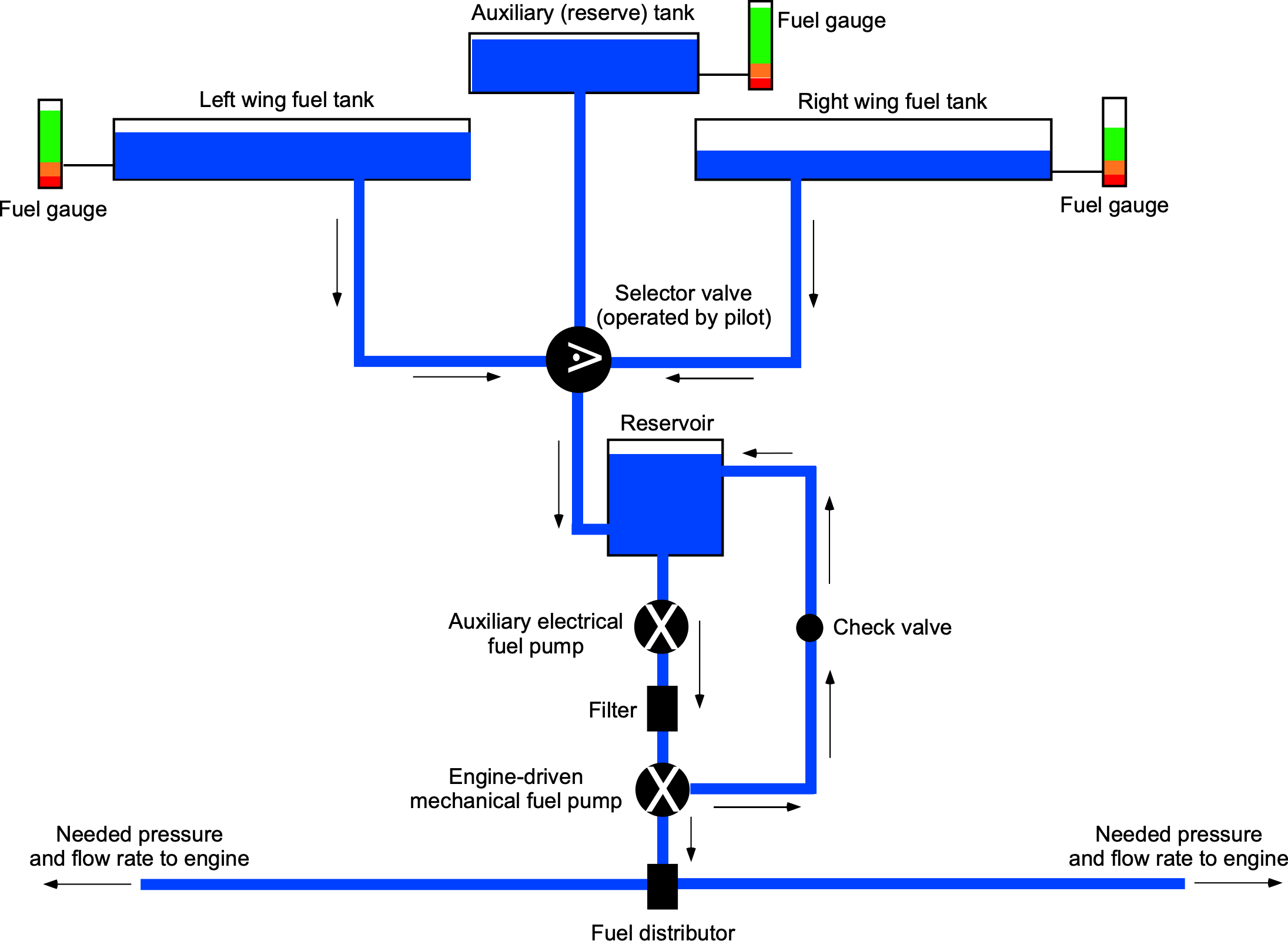
In another example of an internal flow, consider a fuel delivery system on an airplane, where fuel must be pumped from one or more fuel tanks (e.g., located in the wings) to the engine(s), as illustrated in the schematic below. The distribution of the fuel lines also involves considerable lengths, often with many twists and turns through the aircraft structure. Therefore, pressure drops, pumping power, and flow rates must be carefully considered so that the engines receive the required fuel volumes at the pressures necessary to support their requirements. Redundancy of the fuel delivery is achieved in this case through the use of a mechanical (engine-driven) pump and a completely independent backup electrical pump.
An interesting aerospace example of a combined external/internal flow interaction problem was encountered during the design of the X-43A, a hypersonic lifting-body research vehicle. A CFD solution for the flow is shown in the figure below. At hypersonic Mach numbers, the shock waves bend back rather steeply and come close to the fuselage. Hence, the design utilized the lower side of the forward fuselage (an external flow) as part of the engine intake to create the necessary sequence of shock waves, slowing down the air and increasing pressure before it entered the engine’s intake (an internal flow). Therefore, the external flow forms an upstream boundary condition for the internal flow through the engine, allowing it to function correctly.
Categories of Internal Flow Problems
In general, the types of internal flow problems that often arise for aerospace engineers to solve usually fall into these categories:
1. Determining the pressure drop (or the so-called head loss) when flows move through pipes of a given length and diameter for a required volume or mass flow rate.
2. Determining the volume or mass flow rate when the pipe length and diameter are known, given a specified (or allowable) pressure drop, which may be constrained for several reasons.
3. Finding the pumping power needed from a mechanical pump to obtain a certain exit pressure and/or flow rate for a pipe of a specific diameter over a certain length.
4. Determining the pipe diameter when the pipe length and flow or mass rate are known for a particular pressure drop. The pipe size required will also affect its weight and cost, both of which are significant considerations for aerospace applications.
5. Identifying the heating effects of pumping gases through ducts and pipes, especially at higher flow speeds. Heat is generated by frictional losses and gas compression, and heat dissipation may need to be considered in some applications.
Even if most of the relevant information is known, not all of these problems can be solved directly. Design purposes sometimes require iterative solutions starting from initial estimates. However, some fundamental issues illustrating the process of finding pressure drops and determining pumping power through pipes can be introduced.
Fluid Dynamics of Internal Flows
Internal flows are encountered in many shapes and sizes of ducts and pipes, but the flow through a circular pipe is often used as an exemplar, as shown in the figure below. The effects of viscosity cause the fluid in adjacent layers to slow down gradually, progressively developing a velocity gradient in the pipe, i.e., an axisymmetric form of the boundary layer. To compensate for this velocity reduction, the fluid’s velocity at the centerline of the pipe must increase to balance the net mass flow rate through the pipe. Consequently, a significant velocity gradient eventually develops across the entire cross-section of the pipe. The primary manifestation of viscous friction on the interior walls is a pressure drop along the length of the pipe, which depends on the velocity profile, the volumetric or mass flow rate, and the type of fluid.
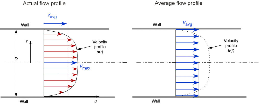
Determining the velocity profile and the corresponding mass (or volume) flow rate is one problem in analyzing internal flows. For example, the average velocity  at some downstream cross-section of a pipe or duct flow can be determined from the velocity profile using the conservation of mass. The mass flow rate
  is given by
(1) 
where  is the pipe’s cross-sectional area, and
  represents the velocity profile in the pipe as a function of the distance
  from the centerline; notice that the profile is assumed to be axisymmetric.
For the incompressible flow in a circular pipe of diameter  and radius
  , then
(2) 
Therefore, if the velocity profile  is known (or the mass flow rate or volume flow rate for an incompressible fluid is given), then the average velocity in the pipe can be determined.
Entrance Length
At the beginning of any internal flow, there is a transition period as it organizes itself to become a fully developed internal flow. As shown in the schematic diagram below, the entrance region or length in such a flow,  , is the length needed to transition to a fully developed internal flow. In the entrance region, the velocity profile changes in the flow direction as it transitions from an initial profile at the inlet to a fully developed profile, where the effects of the walls are felt across the entire cross-sectional area of the pipe, duct, or channel.
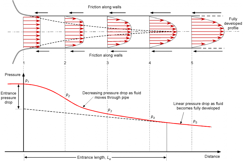
Therefore, a fully developed internal flow is defined as one in which the velocity profile remains constant along the flow direction, i.e., in the axial downstream direction. When the duct has the same cross-section, sections will have the same velocity profile at successive axial locations. If the pipe changes in cross-section or turns a corner, it will take some distance for the flow to fully develop again.
As might be expected, the entrance length depends on whether the flow is laminar or turbulent and whether the internal surface is smooth or rough. For example, for the laminar flow in a smooth, straight cylindrical pipe of diameter , the entrance length is known to be
(3) 
where  is the Reynolds number based on the diameter of the pipe, i.e.,
(4) 
For a fully developed turbulent flow, the entrance length is
(5) 
This latter result indicates that the flow mixing caused by turbulence significantly accelerates the process of achieving a fully developed internal flow.
Under most practical conditions, the flow in a circular pipe is laminar for  and turbulent for
  and will be transitional intermittent in between, i.e., not entirely one state or another. In practice, the lengths of pipes used are generally many times the entrance length, so for most analyses, the assumption that the entire pipe is turbulent is usually reasonable. Of course, these preceding results will change somewhat for different geometries or if the pipe has a bend, turn, or obstruction, such as a pump or flow meter.
Hydraulic Diameter
For flows through non-circular pipes (for which many types are encountered in engineering practice), the Reynolds number is redefined based on the hydraulic diameter  , i.e.,
(6) 
where is the cross-sectional area of the pipe, and  is its wetted perimeter. The hydraulic diameter is sometimes referred to as the hydraulic mean diameter. The basic idea is illustrated in the figure below. Naturally, the hydraulic diameter is defined to reduce to the physical diameter for circular pipes, i.e.,
  .
.
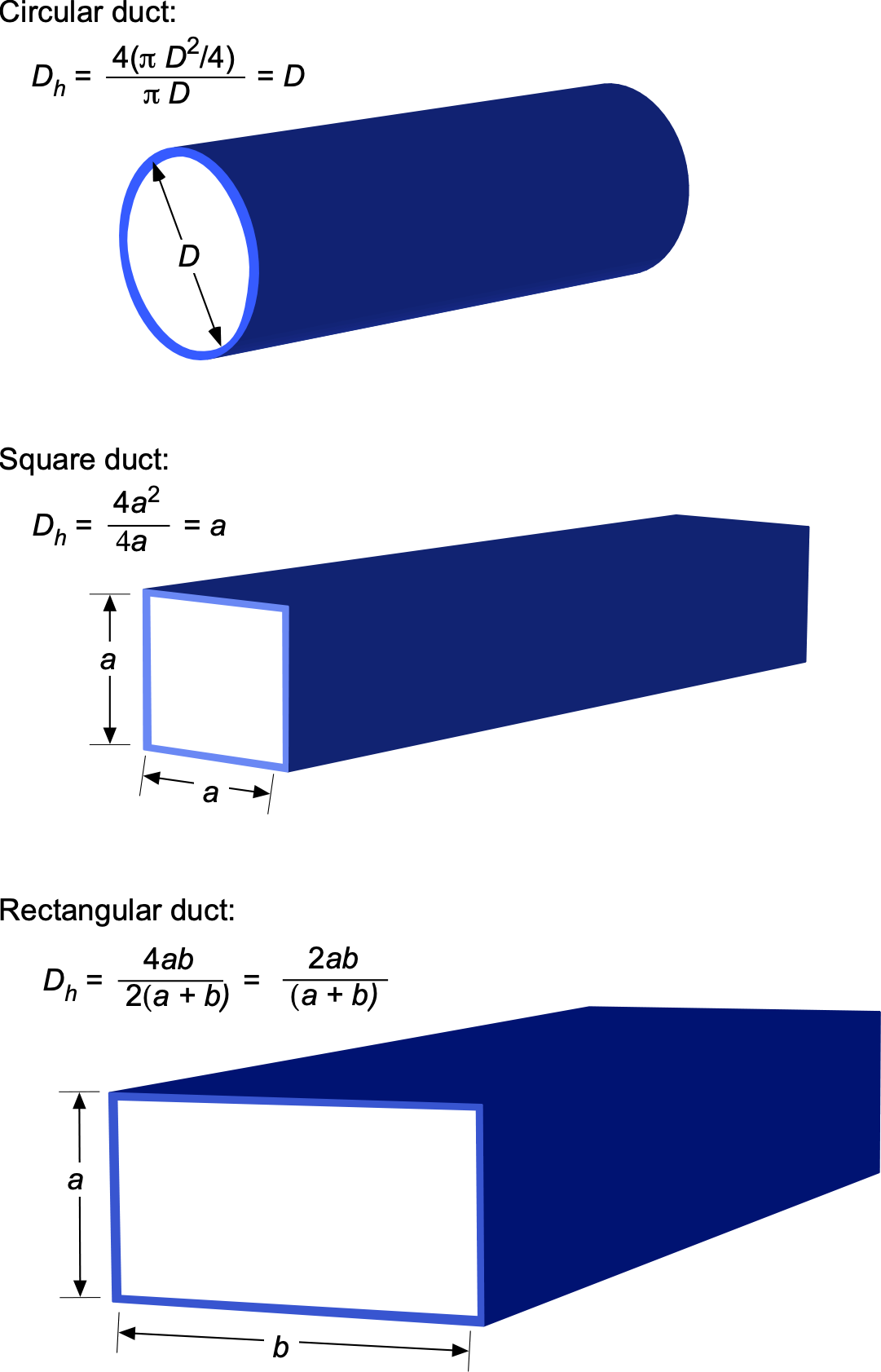
For example, for a pipe with a rectangular cross-section of width  and height
  , the area of the duct is
  , and the perimeter is
  . Therefore, the equivalent hydraulic diameter for this cross-section is
(7) 
Notice that in a square duct where  , then
  .
.
The corresponding Reynolds number will now be calculated by using the hydraulic diameter, i.e.,
(8) 
However, the concept of a hydraulic diameter is most effective for fully developed turbulent flows, i.e., for  greater than approximately 2,000, where the effects of the pipe geometry are less critical.
Laminar Flow in Pipes
Consider the analysis of the steady laminar flow of an incompressible fluid with constant properties in the fully developed region of a smooth straight pipe of circular cross-section. This problem, often referred to as a Hagen-Poiseuille flow, provides one of the few exact solutions for viscous internal flows. Such laminar flows are also sometimes referred to as a class of Poiseuille or Couette flows. The approach is exceptionally instructive and serves as a prerequisite for understanding turbulent flows through pipes, which involves a semi-empirical analysis.
The flow moves at a constant axial velocity in the fully developed laminar flow. The velocity profile remains unchanged with downstream distance, i.e., it is self-similar. It can also be assumed that there is no flow in the radial direction, making this a one-dimensional axisymmetric flow problem. In many cases, the assumption that the flow is steady is reasonable, but it must be justified on a problem-by-problem basis.
Flow Model
Consider an area (annular disk) of the flow at a given pipe cross-section. As shown in the figure below, the forces acting on the annular disk arise from a balance of pressure and viscous (shear) forces. The area of the annular disk is  , and its perimeter is
  . It is assumed that the flow is fully developed.
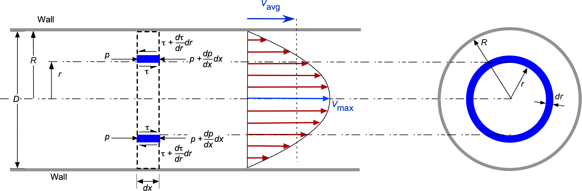
Force equilibrium of the annulus requires a balance of pressure and shear forces such that
(9) 
Expanding out the terms and canceling terms where possible gives
(10) 
Because terms involving  are negligible, then
(11) 
which, after rearrangement and neglecting  terms, leads to
(12) 
or
(13) 
Shear Stresses
The shear stresses are given by Newton’s law of viscosity, such that
(14) 
where the minus sign reflects that the flow velocity decreases with increasing away from the radial centerline, i.e., the gradient is negative. Therefore, the governing equation for this internal flow becomes
(15) 
(16) 
It can be seen that the right-hand side of this equation is a function of the downstream distance  , and the right-hand side is a function of the radial coordinate . The equality in Eq. 16 must hold for any value of and , i.e.,
  can be satisfied only if both
  and
and  are equal to the same constant. Therefore,
  is constant.
Solution to the Governing Equation
Equation 16 can be solved by integrating it twice. Integrating once gives
(17) 
Applying the axisymmetric flow condition that  for
for  is
is  gives
gives  , so
, so
(18) 
Integrating again gives
(19) 
Applying the no-slip condition that  to solve for
  gives
gives
(20) 
Volumetric and Average Flow Rates
The volumetric flow rate is
(21) 
so substituting  and evaluating gives
(22) 
Therefore, the final velocity profile is
(23) 
This is the classic Hagen-Poiseuille flow equation for the fully developed laminar flow in a circular pipe.
For the preceding velocity profile, the average velocity can be determined using
(24) 
which, on substitution, gives
(25) 
Therefore, in terms of , then
(26) 
also noticing that the centerline velocity  , i.e., the average velocity is half the maximum centerline velocity, i.e.,
(27) 
However, this result applies only to this specific case.
Quantifying the Pressure Drop
A quantity of interest in the analysis of internal flows is the pressure drop  , mainly because this drop is directly related to the power requirements of the pump to maintain a certain flow rate through the pipe. Recall that the pressure gradient is constant for a steady flow through a pipe of constant area, so integrating from location 1 where the pressure is
  to another point at a distance
  downstream where the pressure is
  gives
gives
(28) 
Because is given by
(29) 
then
(30) 
Of course, this pressure drop is a direct consequence of the action of viscous effects, so the pressure drop is irrecoverable.
Notice that for a given length of pipe, the pressure drop is proportional to the fluid’s viscosity and flow speed, so the faster a given fluid moves through a pipe or duct, the more significant the pressure drop will be. The pressure drop can also be reduced by using a larger diameter pipe. However, weight and cost are often substantial concerns in aerospace systems, where a trade-off exists between the weight and cost of a larger pipe (to reduce losses) versus a bigger pump (to overcome existing losses). In practice, this pressure drop will also vary for different pipe cross-sections, surfaces (smooth or rough), and other factors.
The pressure loss for a laminar flow can be expressed as
(31) 
where  is called the friction factor. For a fully developed laminar flow in a smooth circular pipe, the friction factor is
(32) 
which depends solely on the Reynolds number. The friction factors for fully developed laminar flow in pipes with other cross-sections, such as square pipes, oval pipes, and triangular pipes, are published in various sources. Still, these latter shapes are rarely encountered in aerospace applications.
The head loss,  , is frequently used in hydraulics to represent the magnitude of the frictional pressure losses,
  . This quantity is equivalent to the additional hydrostatic height that a fluid must be raised to overcome frictional pressure losses. Therefore,
(33) 
After the pressure or head loss is known, the required power  to overcome the pressure loss can be determined from
(34) 
where  is the volume flow rate, and is the head loss height, i.e., the hydrostatic height corresponding to the pressure drop .
The average velocity for the laminar flow in a horizontal pipe (i.e., no gravitational hydrostatic pressure contributions) is
(35) 
so the volume flow rate for laminar flow through the pipe becomes
(36) 
which is known as Poiseuille’s law.[1]
In terms of the pressure drop, then
(37) 
This result means that for a specified flow rate, the pressure drop (and the required pumping power to overcome the losses) is proportional to the pipe’s length and the fluid’s viscosity but inversely proportional to the fourth power of the diameter. This result indicates that even modest increases in pipe diameter can significantly reduce pumping power. However, this approach may not always prove practical (or even possible) for other reasons, including higher weight and costs.
Historical Context – Poiseuille’s Original Equation
Poiseuille did not originally derive the equation now known as Poiseuille’s law, which is accepted as
![\[ \small{Q = \frac{\Delta p \, \pi \, D^4}{128 \, \mu \, L}} \]](https://eaglepubs.erau.edu/app/uploads/quicklatex/quicklatex.com-d90b251f735fc21e9536e9cf2b721362_l3.svg "Rendered by QuickLaTeX.com")
Instead, based on his many meticulous experiments, Poiseuille’s equation for the flow rate in terms of pressure drop was written as
![\[ \small{Q = \frac{K'' \, \Delta p \, D^4}{L}} \]](https://eaglepubs.erau.edu/app/uploads/quicklatex/quicklatex.com-613099664ff33e640b16241827c752fe_l3.svg "Rendered by QuickLaTeX.com")
where  . Poiseuille did not mention viscosity in his work, only indicating that the value of
  depended on temperature. At that time, the understanding of viscosity was tentative, although Navier and Stokes later (independently) rationalized this physical property. The derivation of Poiseuille’s law from the Navier-Stokes equations came later. Poiseuille’s so-called “constant,” , was shown to be
![\[ \small{K'' = \frac{\pi}{128 \, \mu}} \]](https://eaglepubs.erau.edu/app/uploads/quicklatex/quicklatex.com-0246e0dc923b09071988d270b8d3330e_l3.svg "Rendered by QuickLaTeX.com")
Measurements of the values of the dynamic viscosity  (for water) were later found to match Poiseuille’s results, as expressed by
![\[ {\small \mu = \frac{\pi}{128 \, K''}} \]](https://eaglepubs.erau.edu/app/uploads/quicklatex/quicklatex.com-9c32d6fe9fdc545ade019b5812cda80a_l3.svg "Rendered by QuickLaTeX.com")
Check Your Understanding #1 – Using Poiseuille’s Law
How many small-diameter pipes of diameter  of length does it take to discharge the same volume of liquid as a bigger pipe of the same length if the bigger pipe is twice the diameter of the smaller pipes, i.e.,
  ?
?
Show solution/hide solution.
Poiseuille’s law can also be expressed in terms of flow rate as
![\[ Q = \dfrac{\pi \, D^4 \, \Delta p_L}{128 \mu \, L} = \dfrac{\pi \, R^4 \, \Delta p_L}{8 \mu \, L} \]](https://eaglepubs.erau.edu/app/uploads/quicklatex/quicklatex.com-ee0b47070e5061a7c5a2cadecf125c7e_l3.svg "Rendered by QuickLaTeX.com")
Assume that the hydrostatic pressure is the same at the inlet and outlet (discharge) so that = constant. For the same flow rate, then
![\[ Q = \dfrac{\pi \, D_2^4 }{128 \mu \, L} = \dfrac{N \pi \, D_1^4 \, \Delta p_L}{8 \mu \, L} \]](https://eaglepubs.erau.edu/app/uploads/quicklatex/quicklatex.com-c5e769bee658b9e3a2fc404b5ed723a0_l3.svg "Rendered by QuickLaTeX.com")
where  is the number of smaller pipes. Solving for gives
![\[ N = \dfrac{D_2^4}{D_1^4} = \dfrac{2^4 D_1^4}{D_1^4} = 16 \]](https://eaglepubs.erau.edu/app/uploads/quicklatex/quicklatex.com-7710242eb2404ab6581ea0275755c8d0_l3.svg "Rendered by QuickLaTeX.com")
Therefore, the benefits of using a larger pipe become apparent because the flow rate is proportional to  . See the demonstration here.
Recall that the Poiseuille equation (often called the Hagen-Poiseuille equation) is derived under specific assumptions, i.e., laminar, steady, and incompressible flow. When these assumptions are violated, as in turbulent flow and under geometric conditions such as those found in wide or short pipes, the Poiseuille equation may no longer accurately describe the flow behavior. A rule of thumb is that the ratio of the length to the radius of a pipe should be greater than 1/48 of the Reynolds number for the assumption of the Poiseuille law to be valid.
Check Your Understanding #2 – Calculating the pressure drop for laminar flow in a pipe
The design of the fuel delivery system requires a flow through a smooth pipe of 200 m in length and 15 mm in diameter. The required fuel flow rate is 125 kg hr-1. The fluid properties of the fuel are given as  800 kg m-3 and
  0.00164 kg m-1 s-1. All entrance effects should be disregarded. Calculate: 1. The pressure drop along the length of the pipe. 2. The pump’s pressure requirements (in terms of head). 3. The pumping power requirements.
Show solution/hide solution.
The cross-sectional area of the pipe is
![\[ A_c = \frac{\pi D^2}{4} = \frac{\pi \times 0.015^2}{4} = 0.0001767~\mbox{ m${^{2}}$} \]](https://eaglepubs.erau.edu/app/uploads/quicklatex/quicklatex.com-8448629858f6539988e584a293b9d0f2_l3.svg "Rendered by QuickLaTeX.com")
The mass flow rate is given as 125~kg hr = 0.0347~kg s, i.e.,
![\[ \overbigdot{m} = \varrho \, A_c \, V_{\rm av} = 0.0347~\mbox{ kg s$^{-1}$} \]](https://eaglepubs.erau.edu/app/uploads/quicklatex/quicklatex.com-c0b4052c5442a688ff04401bfd8e4edf_l3.svg "Rendered by QuickLaTeX.com")
The average flow velocity in the pipe is
![\[ V_{\rm av} = \frac{\overbigdot{m}}{\varrho \, A_c} = \frac{0.0347}{800.0 \times 0.0001767} = 0.246~\mbox{m s$^{-1}$} \]](https://eaglepubs.erau.edu/app/uploads/quicklatex/quicklatex.com-64bc6342b4b77f9868aa2cc785e1b6a9_l3.svg "Rendered by QuickLaTeX.com")
The Reynolds number based on pipe diameter is
![\[ Re = \frac{\varrho V_{\rm av} \, D}{\mu} = \frac{ 800.0 \times 0.246 \times 0.015}{0.00164} = 1,797 \]](https://eaglepubs.erau.edu/app/uploads/quicklatex/quicklatex.com-b7b01f2406ef73146e6bb9b15e658633_l3.svg "Rendered by QuickLaTeX.com")
Notice that this Reynolds number is in the laminar regime, so the friction factor is given by
![\[ f = \frac{64}{Re} = \frac{64}{1,797} = 0.0356 \]](https://eaglepubs.erau.edu/app/uploads/quicklatex/quicklatex.com-7958a552eb65dc8a3cd9644e518ec4ff_l3.svg "Rendered by QuickLaTeX.com")
The pressure drop is given by
![\[ \Delta p = \frac{1}{2} \varrho \, V_{\rm av}^2 \, f \left( \frac{L}{D} \right) \]](https://eaglepubs.erau.edu/app/uploads/quicklatex/quicklatex.com-76ae22e8d21c1ba13738eb88f38da9cf_l3.svg "Rendered by QuickLaTeX.com")
and inserting the given values leads to
![\[ \Delta p = \frac{1}{2} \times 800.0 \times 0.246^2 \times 0.0356 \times \frac{200}{0.015} = 11,490.0~\mbox{ Pa} = 11.46~\mbox{kPa} \]](https://eaglepubs.erau.edu/app/uploads/quicklatex/quicklatex.com-04ef5b79ba93ec595c5540e82628a059_l3.svg "Rendered by QuickLaTeX.com")
The equivalent head loss,  , will be
![\[ h = \frac{\Delta p}{\varrho \, g} = \frac{11,490.0}{800.0 \times 9.81} = 1.46~\mbox{ m} \]](https://eaglepubs.erau.edu/app/uploads/quicklatex/quicklatex.com-0ab8a9b5d3d4ad90858251e54bf87710_l3.svg "Rendered by QuickLaTeX.com")
Finally, the pumping power can be determined from
![\[ P = \frac{\overbigdot{m} \, \Delta p}{\varrho} = \frac{0.0347 \times 11,490.0}{800.0} = 0.498~\mbox{W} \]](https://eaglepubs.erau.edu/app/uploads/quicklatex/quicklatex.com-240aed802a6f4d476933e87a5d3e5e00_l3.svg "Rendered by QuickLaTeX.com")
Turbulent Flows in Pipes
Unlike laminar flows, the expressions for the losses in pipes or ducts containing a turbulent flow are based on analysis and measurements, providing empirical or semi-empirical relationships. In fact, because of the importance of many industrial applications, systematic experiments have been performed with pipe flows to measure pressure losses for different flow rates, Reynolds numbers, and surface roughness values.
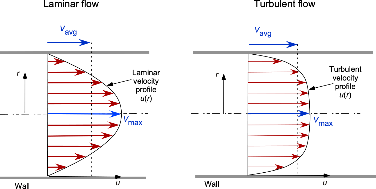
Representative relative velocity profiles for fully developed laminar and turbulent flows are shown in the figure below. Remember that the fully laminar velocity profile is parabolic in laminar flow. However, the profile shape is much “fuller” in turbulent flow because of the mixing between fluid layers, with a more uniform centerline velocity and a sharper drop in flow velocity near the pipe wall. Of course, this characteristic is much like a turbulent boundary layer profile as it develops over an external surface.
Any irregularity or “roughness” on the surface of the pipe, as shown in the figure below, will disturb the development of the boundary layer and create higher wall stresses. Therefore, the friction factor in a pipe flow with turbulence depends on the internal surface roughness, and pipes with greater roughness will result in more significant pressure drops. The roughness,  , is a property of the pipe material.
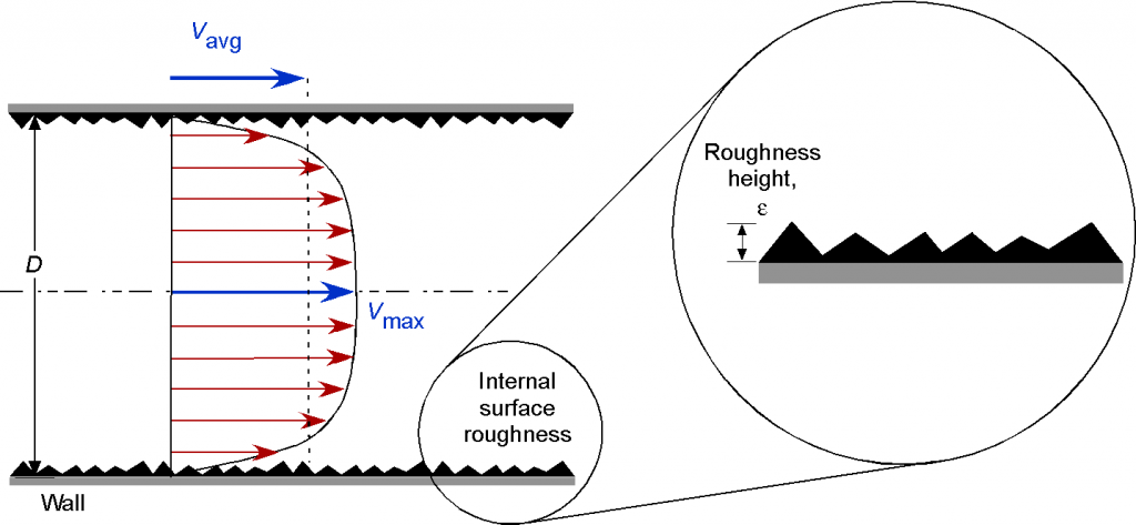
It should be appreciated that “roughness” is a relative concept. In practice, roughness only becomes significant when the height of the roughness elements reaches the thickness of the laminar sublayer, although this layer is relatively small. Many extruded plastic pipes are generally considered hydrodynamically smooth. However, most other surfaces are rough to some degree, so this roughness causes the boundary layer to become turbulent quicker, i.e., after a shorter downstream development distance.
The pressure loss with a turbulent flow is still given by
(38)
but now, the value of cannot be obtained from theoretical analysis. Indeed, the friction factor in fully developed turbulent pipe flows (sometimes called the Darcy-Welsbach friction factor or just the Darcy friction factor) depends on the Reynolds number and the relative roughness height  , which is the ratio of the mean height of roughness of the pipe to the pipe diameter , i.e., for the friction factor then
(39) 
which can also be found from the process of dimensional analysis.
All available results for pressure drops and friction factors for turbulent flows through pipes are obtained from experiments using artificially roughened surfaces. These experiments utilize particle grains of a known size bonded to the inner surfaces of the pipes. Ludwig Prandtl and his students conducted the first such experiments in the 1930s, but generations of hydraulic engineers have performed many more experiments since then. The resulting friction factor is calculated from the flow rate measurements and the pressure drop.
Pipe friction factors can be presented in tabular, graphical, or functional forms, which are obtained by fitting a curve to the measured data. Commercially available pipes are evaluated based on equivalent roughness values, enabling engineers to make accurate calculations for design and installation purposes. However, the relative roughness of the pipe may increase with everyday use because of corrosion or abrasion (depending on the fluid), so friction factors may change over time. Good engineering practice would always account for such effects, ensuring that the required pressure at the end of the pipe can be maintained for its expected service life.
Colebrook-White Equation
The most widely used equation for determining the friction factor in turbulent pipe flows is the Colebrook-White equation. This equation lacks a theoretical basis and is based solely on curve fitting to measurements. The equation is given by
(40) 
where is the pipe roughness, is the hydraulic diameter, and  is the Reynolds number based on . Notice that the Colebrook-White equation is an implicit function of (i.e., the value of appears on both the left- and right-hand sides), requiring an iterative numerical solution. The procedure is easily programmed in MATLAB, and convergence is rapid.
Moody Chart
Most of the available results for turbulent flows through common types of rough pipes have been summarized in the form of a Moody Chart, an example of which is shown below. Engineers can use this chart to calculate the friction factor for a given internal flow along a pipe. The friction factor is then used to calculate the pressure loss, pumping power, and other related quantities. Lewis Moody solved the Colebrook-White equation to create this type of chart, combining the dimensional terms of roughness, , and pipe diameter, , into a non-dimensional relative roughness,  , and the Reynolds number to find the friction factor.
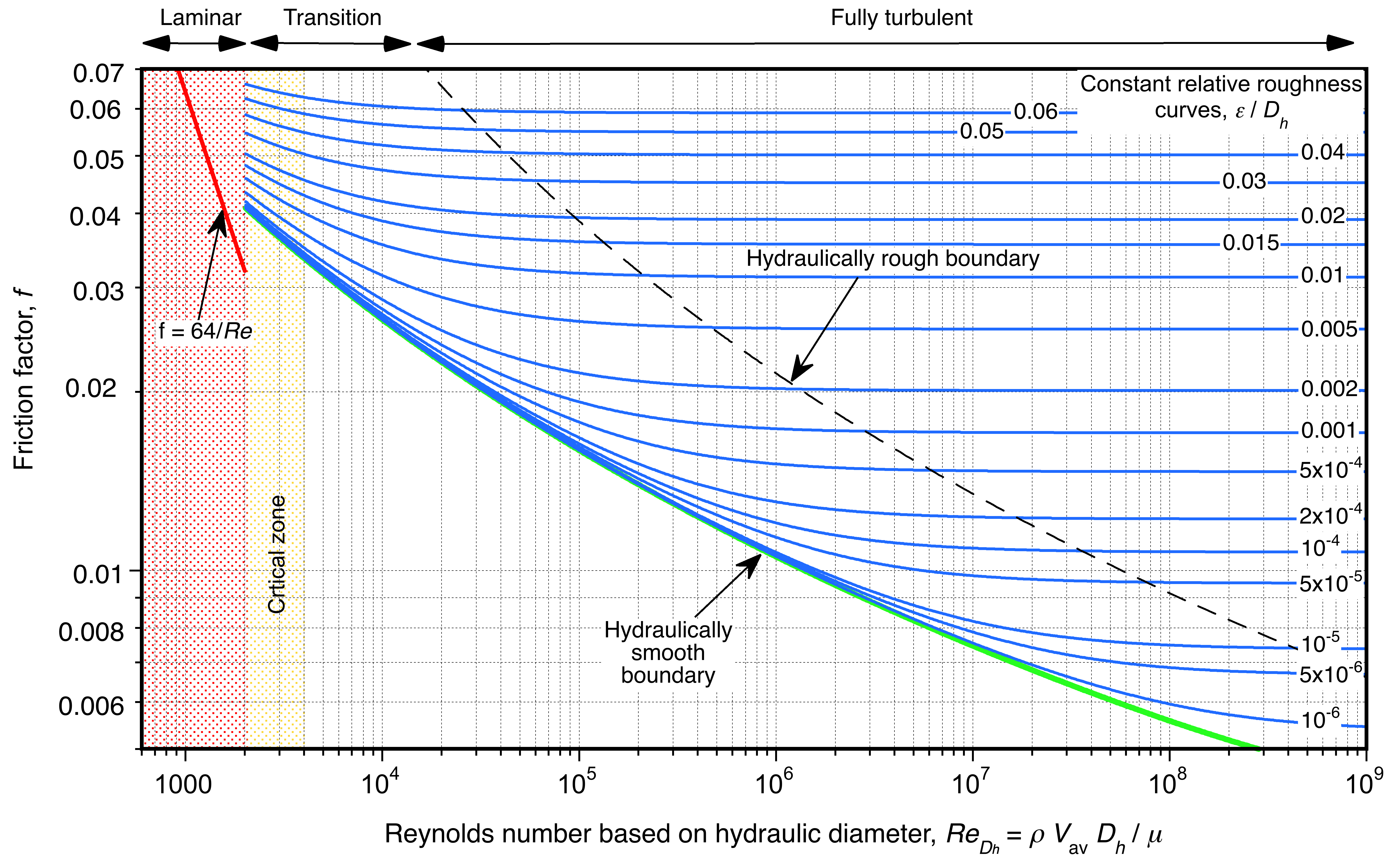
On the Moody Chart, the friction factor, , is on the left-hand side ordinate, the Reynolds number based on diameter (or hydraulic diameter), and the average flow velocity, , is on the abscissa. Notice that the chart has a log-log scale. Curves of constant values of relative roughness, , are then plotted, which are represented by the blue lines shown on the chart. Notice that the right side of the graph is not on a scale. Online calculator versions of the chart are also available; however, some may use approximations to the Colebrook-White equation rather than iteratively solving the actual equation.
Although the Moody Chart was initially developed for flows through circular pipes, it can also be used for non-circular pipes by replacing the circular diameter, , with the equivalent hydraulic diameter, , as previously discussed. Experience suggests that this approach is sufficiently accurate for calculating the pressure drop along non-circular pipes when the flow is fully turbulent.
Remember that the Reynolds number based on diameter or hydraulic diameter is calculated using
(41)
with the fluid properties being represented in terms of density,  , and viscosity, , or the kinematic viscosity,
  (=
(= ). The average flow velocity, , can be calculated from the volume flow rate, , and the area of the cross-section, , i.e.
(42) 
When using the Moody chart, if the values of two of the three parameters are known, i.e., the friction factor, and/or the Reynolds number, , and/or the relative roughness, , then the third parameter may be determined using this chart. However, in practice, the Reynolds number and the relative roughness are usually known or calculated values, so the friction factor is the desired output from reading the chart.
MATLAB code to create the Moody chart using the Colebrook-White equation
Show code/hide code.
% Moody Chart in MATLAB
clear; clc;
% Define the Reynolds number range
Re = logspace(3, 8, 500); % Reynolds number from 10^3 to 10^8
% Define the relative roughness values (epsilon/D)
rel_roughness = [0, 0.00001, 0.0001, 0.001, 0.01, 0.02, 0.05];
% Preallocate friction factor array
friction_factors = zeros(length(rel_roughness), length(Re));
% Calculate friction factors using the Colebrook equation
for i = 1:length(rel_roughness)
for j = 1:length(Re)
if Re(j) < 2000
% Laminar flow
friction_factors(i, j) = 64/Re(j);
else
% Turbulent flow using Colebrook-White equation
f = 0.02; % Initial guess for f
while true
f_new = 1 / (-2*log10((rel_roughness(i)/3.7) + (2.51/(Re(j)*sqrt(f)))));
if abs(f_new – f) < 1e-6
break;
else
f = f_new;
end
end
friction_factors(i, j) = f_new;
end
end
end
% Plot the Moody chart
figure;
loglog(Re, friction_factors, ‘LineWidth’, 2);
hold on;
% Laminar flow line
Re_laminar = Re(Re < 2000);
friction_laminar = 64 ./ Re_laminar;
loglog(Re_laminar, friction_laminar, ‘k–‘, ‘LineWidth’, 2);
% Annotate plot
grid on;
xlabel(‘Reynolds Number, Re’);
ylabel(‘Friction Factor, f’);
title(‘Moody Chart’);
legend(arrayfun(@(x) sprintf(‘\\epsilon/D = %g’, x), rel_roughness, ‘UniformOutput’, false), ‘Location’, ‘Best’);
set(gca, ‘XScale’, ‘log’, ‘YScale’, ‘log’);
xlim([1e3 1e8]);
ylim([1e-3 1]);
% Add text annotations
text(2e3, 0.08, ‘Laminar Flow’, ‘FontSize’, 12, ‘Rotation’, -45);
text(1e7, 0.008, ‘Turbulent Flow’, ‘FontSize’, 12);
% Add grid lines for guidance
set(gca, ‘MinorGridLineStyle’, ‘-‘, ‘GridAlpha’, 0.5, ‘MinorGridAlpha’, 0.5);
hold off;
Interpretation
The following points should be understood when using and interpreting the curves on the Moody chart:
1. The laminar flow line represents a lower theoretical bound of the friction factor for low Reynolds numbers, i.e.,
(43) 
There are few practical situations where this is a valid assumption other than for very short, smooth pipes and ducts. Nevertheless, the result shows that the friction factor decreases with increasing Reynolds number, and there is no dependency on surface roughness.
2. The shaded area indicates a critical zone. This is where the flow begins to develop turbulence, but is unsteady and intermittent in its flow characteristics. The friction factor can exhibit significant changes in this region, indicating that the flow in this area may be either laminar or turbulent. The empirical data here are limited in scope and show considerable scatter. Fortunately, it is uncommon to have to use this part of the chart.
3. The friction factors increase with surface roughness for any given Reynolds number; at higher Reynolds numbers, this is a rather obvious expectation. Notice that even entirely smooth pipes containing a turbulent flow, such as plastic and glass, which have values of or  , will still have a friction factor and a pressure drop along their length, but these effects continue to diminish with increasing Reynolds number.
4. At higher Reynolds numbers, which is called the fully turbulent or hydraulically rough zone, the friction factors become nearly independent of the Reynolds number. This behavior occurs because the protruding roughness penetrates deeply into the boundary layer, extending beyond any laminar sublayer, ensuring that the internal flow remains fully turbulent. Notice that this zone (boundary) occurs at an increasingly higher Reynolds number with lower roughness factors. Moody defined the boundary of the hydraulically rough zone as
(44) 
Using Eq. 40, it can be shown that
(45) 
Therefore, the hydraulically rough boundary (black dashed line on the Moody chart) can be approximated by the equation
(46) 
5. When the relative roughness becomes even higher, i.e., when  , the values of the friction factor become independent of the Reynolds number at any Reynolds number. In such cases, the friction factors become horizontal lines. Because of the large pressure drops associated with flows through pipes with such high roughness levels, they are of no practical significance.
Reading a Moody Chart
Reading a Moody chart is not difficult, but it requires some practice, as it is a log-log chart that necessitates graphical interpolation. While the friction factor can be calculated numerically using the Colebrook-White equation, it is still essential to understand the visual interpretation of the physical behavior and the process of using the chart, as shown in the example below. Reading the chart to three decimal places is more than adequate. Notice that some published Moody charts, such as those found on the internet, may give slightly different friction factor values because they are based on approximations to the Colebrook-White equation.

In this case, it is assumed that the information needed to calculate the Reynolds number and the relative roughness is available, and the desired output is the friction factor, .
- Determine the Reynolds number based on the average flow velocity, , and fluid properties ( and or ) using the hydraulic diameter, , of the pipe, i.e.,
![\[ Re_{D_{h}} = \frac{\varrho \, V_{\rm av} \, D_h}{\mu} = \frac{V_{\rm av} \, D_h}{\nu} \]](https://eaglepubs.erau.edu/app/uploads/quicklatex/quicklatex.com-4e38b80fcdca9e8d518a33ac44e98429_l3.svg "Rendered by QuickLaTeX.com")
where the average flow velocity is determined from the flow rate and cross-sectional area, i.e.,
![\[ V_{\rm av} = \frac{Q}{A_c} \]](https://eaglepubs.erau.edu/app/uploads/quicklatex/quicklatex.com-a8a7d55dc82b4a5fb4c9a2ff778ef5dd_l3.svg "Rendered by QuickLaTeX.com")
- Calculate the value of the relative roughness from the actual dimensional roughness, , and calculated hydraulic diameter, , i.e.,
![\[ \mbox{\small Relative roughness} = \frac{\epsilon}{D_h} \]](https://eaglepubs.erau.edu/app/uploads/quicklatex/quicklatex.com-07f508147b73db06c557e15290911f79_l3.svg "Rendered by QuickLaTeX.com")
The roughness value,
, is often stamped on industrial piping or can be found in widely published standard tables. - Find the appropriate (blue) curve for the calculated value of relative roughness on the Moody diagram, recognizing that only a finite number of curves can be shown, and interpolation of the curves on the logarithmic scales will likely be required.
- Find where the friction factor curve (or interpolated curve) intersects the Reynolds number (at the red dot).
- Estimate the friction factor by reading the value on the vertical scale on the ordinate to the left of the red dot point, from where the Reynolds number and relative roughness curve intersect.
Finally, some words of caution are appropriate when using the Moody Chart. First, as with all engineering calculations, ensuring that the correct units are consistently used when calculating non-dimensional quantities, such as the Reynolds number and relative roughness, is crucial. Ensure that the Reynolds number is calculated based on the pipe’s diameter (or hydraulic diameter), not its length. Catastrophic mistakes can occur if the correct units are not used with care and consistency. Second, because of the numerous lines on the chart, it is essential to interpolate carefully. The human eye/brain combination is a suitable interpolator, but greater accuracy may be required. In this case, the Colebrook-White equation can be solved directly, or an accepted approximation can be used.
Approximations for the Friction Factor
The von Kármán rough pipe law, also known as the von Kármán-Prandtl roughness law, is an empirical relationship used to estimate the friction factor for a fully developed turbulent fluid flow through a pipe with rough walls. It can be written as
(47) ![\begin{equation*} \frac{1}{\sqrt{f}} = -2.0 \, \log_{10}\left[ \left( \displaystyle{\frac{\epsilon}{3.7 D_h}}\right) + \frac{2.51}{Re_{D_{h}}\sqrt{f}}\right] \end{equation*}](https://eaglepubs.erau.edu/app/uploads/quicklatex/quicklatex.com-84c63489e9636bd192ad8a9fe209b23c_l3.svg "Rendered by QuickLaTeX.com")
which is, again, an implicit equation that must be solved by iteration. While only approximate, it applies to a wide range of Reynolds numbers and roughness factors.
The Swamee-Jain equation, also known as the Swamee-Jain friction factor equation, can also be used to calculate the friction factor, , for internal fluid flow. The equation is a simplified form of the von Kármán rough pipe law and provides an explicit approximation for the friction factor, i.e.,
(48) ![\begin{equation*} f = \frac{0.25}{\left[\log_{10}\left( \displaystyle{ \frac{\epsilon}{3.7 D_h} + \frac{5.74}{Re_{D_{h}}^{~0.9}}} \right)\right]^2} \end{equation*}](https://eaglepubs.erau.edu/app/uploads/quicklatex/quicklatex.com-eee1b0e1bbcdca1e1c745b5b20f6427c_l3.svg "Rendered by QuickLaTeX.com")
Roughness Values
In most cases, roughness values cover a range and will depend on the specific surface, as shown in the table below. As manufactured, the roughness values will be on the lower end of the scale; however, all types of pipes may develop some roughness over time due to oxidation or corrosion. It is always essential to consult relevant standards and specifications, or obtain specific roughness values, for the particular pipe(s) used in a given application.
| Pipe Material | Roughness, ε (mm) |
|---|---|
| Smooth Plastic (PVC) | 0.001 – 0.01 |
| Glass | 0.001 – 0.01 |
| Smooth Metal (e.g., SS) | 0.001 – 0.03 |
| Concrete | 0.2 – 1.5 |
| Galvanized Iron | 0.15 – 0.5 |
| Commercial Steel | 0.045 – 0.09 |
| Riveted Steel | 0.9 – 1.2 |
| Corrugated Metal | 3.0 – 8.0 |
| Cast Iron (new) | 0.15 – 0.5 |
| Cast Iron (old) | 0.6 – 3.0 |
| Smooth Copper | 0.001 – 0.01 |
| Polyethylene (PE) | 0.001 – 0.01 |
| Polyvinyl Chloride (PVC) | 0.001 – 0.01 |
| Fiberglass | 0.01 – 0.03 |
| Stainless Steel (welded) | 0.025 – 0.05 |
| Stainless Steel (seamless) | 0.02 – 0.045 |
| Aluminum | 0.05 – 0.1 |
| Brass | 0.02 – 0.05 |
| PVC (Corrugated) | 1.5 – 3.0 |
| HDPE (Corrugated) | 0.4 – 1.5 |
| Ductile Iron | 0.025 – 0.05 |
| Polypropylene | 0.01 – 0.03 |
| ABS | 0.02 – 0.06 |
Check Your Understanding #3 – Calculating the pressure drop for turbulent flow in a pipe using the Moody chart
Oil with a density  kg/m
kg/m and kinematic viscosity
  m
m /s, flows at 0.2 m/s through a 500 m length of 300 mm diameter cast iron pipe. The average roughness of the pipe’s surface is 0.26 mm. Calculate: 1. The average flow velocity in the pipe. 2. The Reynolds number of the flow. 3. Is the flow in the pipe laminar or turbulent? 4. The pressure drop and head loss along the pipe. 5. The minimum power of the pump needed to move the oil.
Show solution/hide solution
- The average flow velocity is calculated from the volume flow rate, i.e.,
![\[ V_{\rm av} = \frac{Q}{A }= \frac{4Q}{\pi D^2} = \frac{4 \times 0.2}{\pi \times 0.3^2} = 2.83~\mbox{ m/s} \]](https://eaglepubs.erau.edu/app/uploads/quicklatex/quicklatex.com-a9561d0c2bdc0bcf3048c17a05f734dc_l3.svg "Rendered by QuickLaTeX.com")
- The Reynolds number of the flow in the pipe is
![\[ Re_{_{D}} = \frac{\varrho_{\rm oil} \, V_{\rm av} \, D}{\mu_{\rm oil} } =\frac{V_{\rm av} \, D}{\nu_{\rm oil}} = \frac{2.83\times 0.3 }{10^{-5}} = 84,900 \]](https://eaglepubs.erau.edu/app/uploads/quicklatex/quicklatex.com-c9182af151a981ce2779bf1ef70c2627_l3.svg "Rendered by QuickLaTeX.com")
- The flow will be turbulent because the Reynolds number is greater than 2,000, and the Moody chart will be needed to find the friction factor .
- To find the pressure drop and use the Moody chart, the relative surface roughness is needed, which is
![\[ \frac{\epsilon}{D} = \frac{0.26}{300} = 0.00087 \]](https://eaglepubs.erau.edu/app/uploads/quicklatex/quicklatex.com-29580f4659e5ff11b395dbd34fd1591d_l3.svg "Rendered by QuickLaTeX.com")
From the Moody chart for a Reynolds number of 84,900 and a relative roughness of 0.00087 (using interpolation), then
 . Notice: You may get a slightly different number for the friction factor depending on the Moody chart you use. Therefore, the pressure loss over the length of the pipe is
![\[ \Delta p = \frac{1}{2} \varrho_{\rm oil} \, V_{\rm av}^2 \, f \left( \frac{L}{D}\right) = 0.5\times 900\times 2.83^2 \times 0.022\times \frac{500}{0.3} = 132.15~\mbox{ kPa} \]](https://eaglepubs.erau.edu/app/uploads/quicklatex/quicklatex.com-7396bd04be8c55c6c89a30055eaafee2_l3.svg "Rendered by QuickLaTeX.com")
The corresponding head loss over this pipe is
![\[ h = \frac{\Delta p}{\varrho_{\rm oil} \, g} = \frac{132.15\times 10^3}{900\times 9.81} = 14.97~\mbox{m} \]](https://eaglepubs.erau.edu/app/uploads/quicklatex/quicklatex.com-b2f2f6a68881520d5549eba4f4a0dccf_l3.svg "Rendered by QuickLaTeX.com")
- The pumping power required will be
![\[ P_{\rm req} = Q \, \Delta p = 0.2 \times 132.15 \times 10^3 = 26.43~\mbox{kW} \]](https://eaglepubs.erau.edu/app/uploads/quicklatex/quicklatex.com-a40c927b1a3a73383e2fe118876d3db5_l3.svg "Rendered by QuickLaTeX.com")
Pressure Drop Over a Tapered Pipe
There are no exact solutions for the pressure drop along a tapered pipe; an example of such a shape is shown in the figure below. The main issue is that the flow velocity and Reynolds number vary continuously. However, numerical solutions may be possible where the local losses over short segments are added to determine the local losses in aggregate. In the case of fully turbulent flow with higher Reynolds numbers where the friction factor becomes independent of Reynolds number, the pressure drop can be estimated using the concept of a hydraulic diameter and average flow velocity.
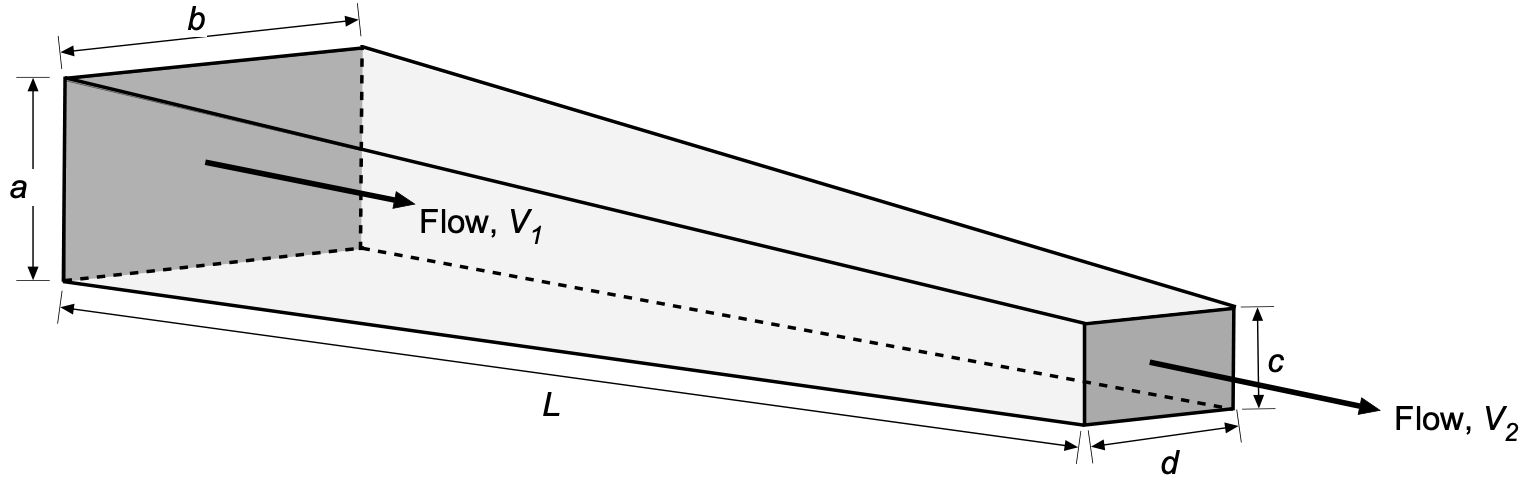
In this case, the average hydraulic diameter is
(49) 
The average flow velocity, , based on continuity considerations is given by
(50) 
The Reynolds number based on the average hydraulic diameter and average flow velocity can then be obtained, i.e.,
(51)
Then the Moody chart can be used with the relative roughness to get the friction factor, , or the Swamee-Jain equation can also be used, i.e.,
(52)
Therefore, the pressure loss over the length of tapered pipe will be
(53) 
These pressure drop estimates are sufficiently accurate for many practical purposes, including wind tunnel design.
Pumps
Many internal flow problems involve using or designing various types of pumps to move fluid from one place to another. Such pumps include hydraulic pumps, piston pumps, centrifugal pumps, gear-type pumps, vane pumps, axial flow pumps, fans, etc. For aerospace applications, pumps must be lightweight (i.e., high power-to-weight ratio), reliable, and often contend with harsh operating environments, including large temperature swings and vibration. Pumps obtained “off-the-shelf” are usually specified in terms of their volumetric transfer capacity per unit time. It is essential to notice the units in which the volumetric flow rates are given, which will typically not be in base units; e.g., they may be quoted in terms of liters/hr, gallons/minute, or other units.
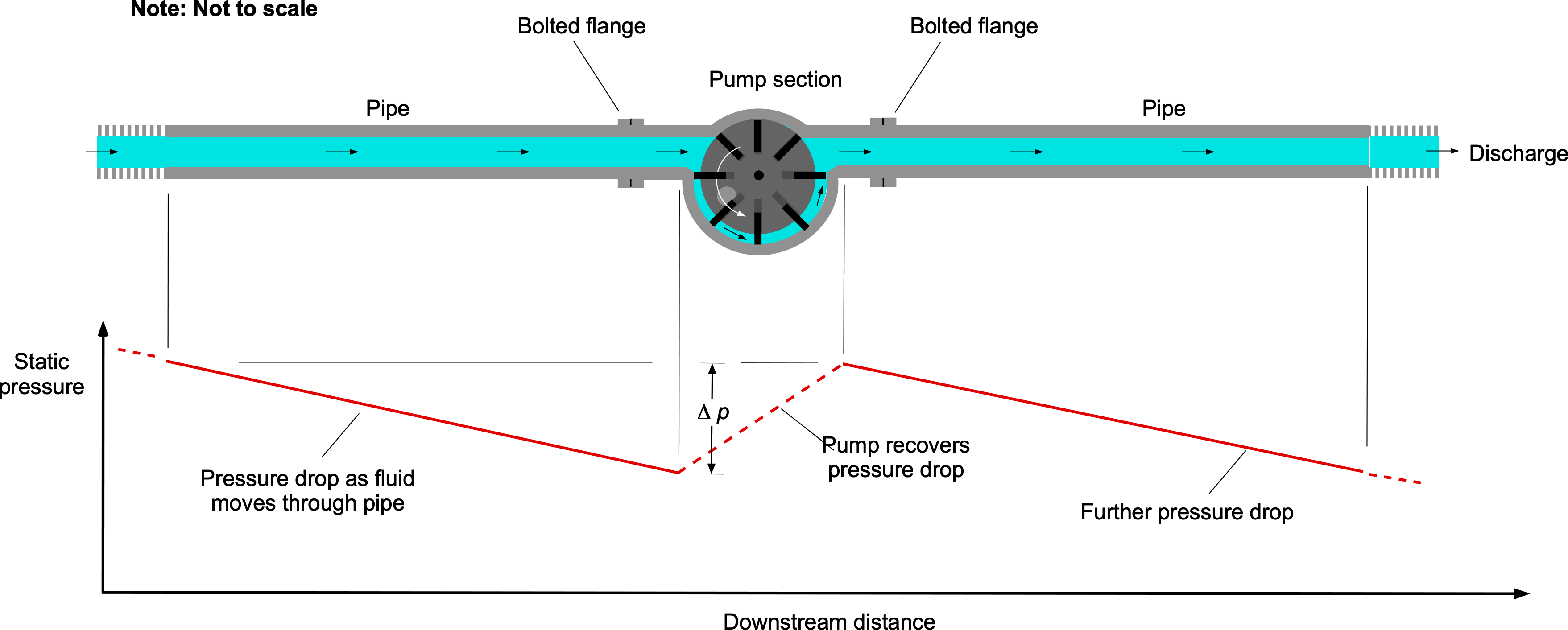
In general, pumps recover pressure losses so fluid can be pumped from one location to another, as shown in the figure below. Any pump will produce the same effect of pressure recovery, although with different efficiencies and applicabilities to different types of fluids. Pressure drops depend on several factors, including the flow rate, Reynolds number, and friction factor.
Types of Pumps
The figure below shows four common types of fluid pumps: a gear pump, lobe pump, vane pump, and centrifugal pump. In each case, the pumps must be rotated by a power source. This source could be an accessory drive through a belt or gear system from an engine or propulsion system or a direct drive from a separate source such as an electric motor. Such pumps are usually inserted in series into a pipeline and bolted to the pipe using parallel flanges sealed by a gasket.
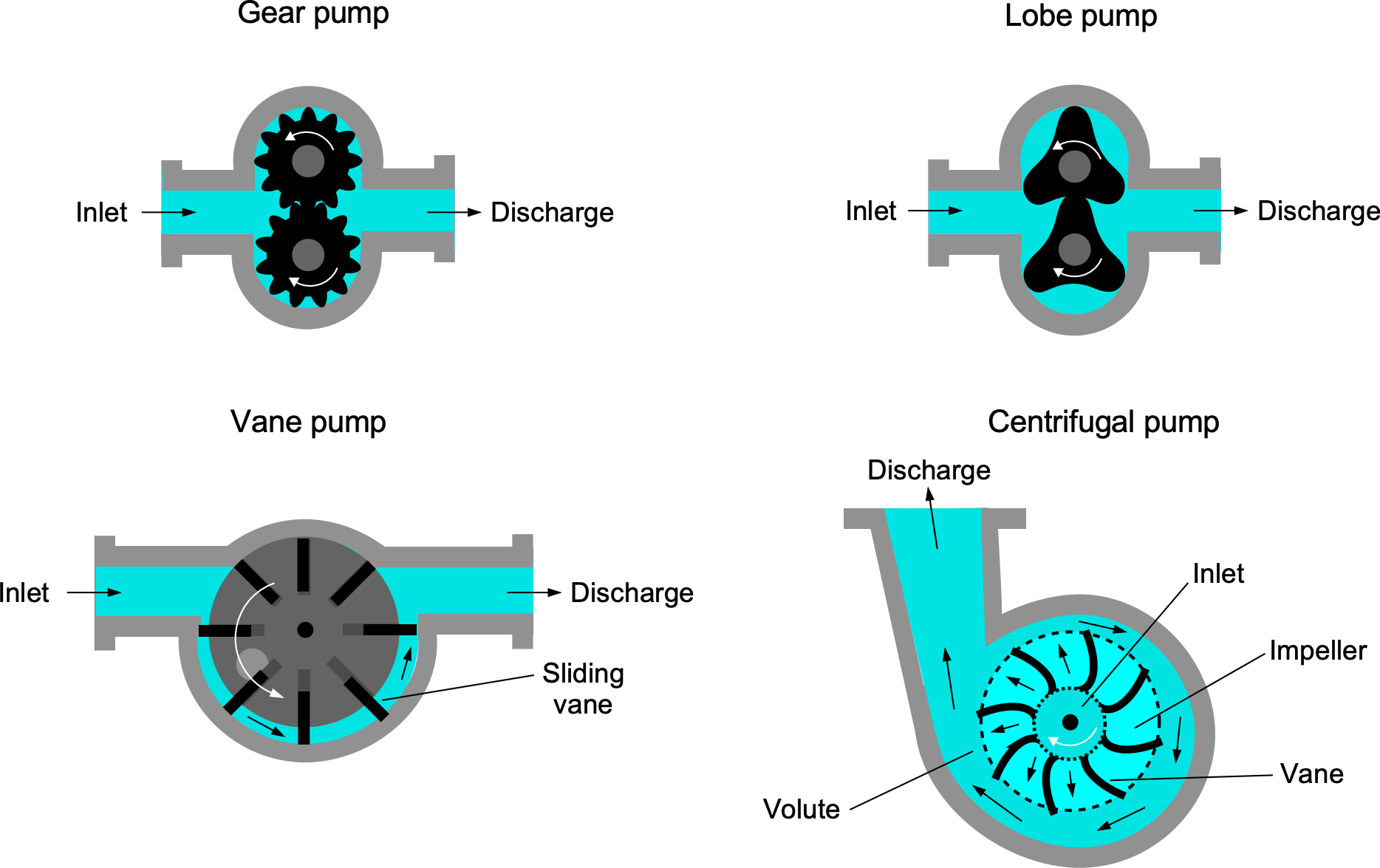
Gear Pumps
Gear pumps are positive displacement pumps that utilize two meshing gears to transfer fluids by creating chambers between the gear teeth and the pump casing. They come in various types, external and internal, offering specific advantages and applications. Gear pumps are valued for their simplicity, reliability, and ability to handle various viscosities, making them suitable for applications in industries such as hydraulic systems, lubrication systems, and fuel transfer. Lubrication systems in engines often use gear pumps because of their simplicity, low cost, and good reliability.
Lobe Pumps
Lobe pumps are positive displacement pumps characterized by two or more lobes that rotate in synchronized motion within a casing, creating chambers that transport fluid from the inlet to the outlet. Unlike gear pumps, lobe pumps feature smooth meshing lobes instead of gears, offering smoother, more efficient fluid flow with lower losses. They are widely used because they can handle more viscous fluids, such as oils. They are reliable but tend to be more expensive than gear pumps.
Vane Pumps
Vane pumps are positive displacement pumps that employ rotating vanes inside a cylindrical housing to move fluid from the inlet to the outlet. These pumps typically feature an off-center drive to the vanes. The vanes are often made of carbon, causing them to slide in and out of their slots while maintaining close contact with the housing. Vane pumps have a smooth and consistent flow, making them suitable for applications requiring precise and steady fluid delivery, such as hydraulic and pneumatic systems. They offer relatively quiet operation and can handle various viscosities, though they experience reduced efficiency for more viscous fluids. Furthermore, the vanes wear over time and require periodic maintenance to ensure their functionality.
Centrifugal Pumps
Centrifugal pumps utilize centrifugal forces on the fluid to increase the fluid’s rotational kinetic energy. Such pumps consist of an impeller enclosed within a casing, propelling the fluid outward from the center of rotation. The fluid is introduced through a pipe at the center of the pump. As the fluid moves through the pump, it gains velocity and pressure, transferring fluid from the inlet to the outlet. Centrifugal pumps are widely used in applications requiring high flow rates. While efficient, they tend to be better suited for gases rather than more viscous liquids.
Diaphragm pump
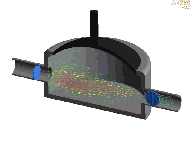
The figure below shows a CFD simulation of the internal flow through a diaphragm pump or membrane pump. In this type of pump, which is common in fuel delivery systems, the diaphragm is flexed up and down (by a motor) such that when the volume of the chamber is increased, the pressure decreases, the fluid is drawn from one end of the pipe into the chamber. When the chamber pressure rises from the reduced volume, the fluid previously drawn in is forced through the other pipe. Notice that a pair of butterfly valves prevent reverse fluid flow from the pump.
Pressure Drops Over Bends & Corners
When an internal fluid flow encounters a corner or bend, it experiences a pressure drop from the change in direction, as shown in the figure below. Several factors, including centrifugal forces, changes in velocity, and the possibility of flow separation, cause this pressure drop. As the fluid approaches the corner, it tends to move outward under the action of centrifugal forces, which creates a pressure gradient across the cross-section of the corner or bend. If the corner is sharp, the flow separation and higher pressure losses can be expected.
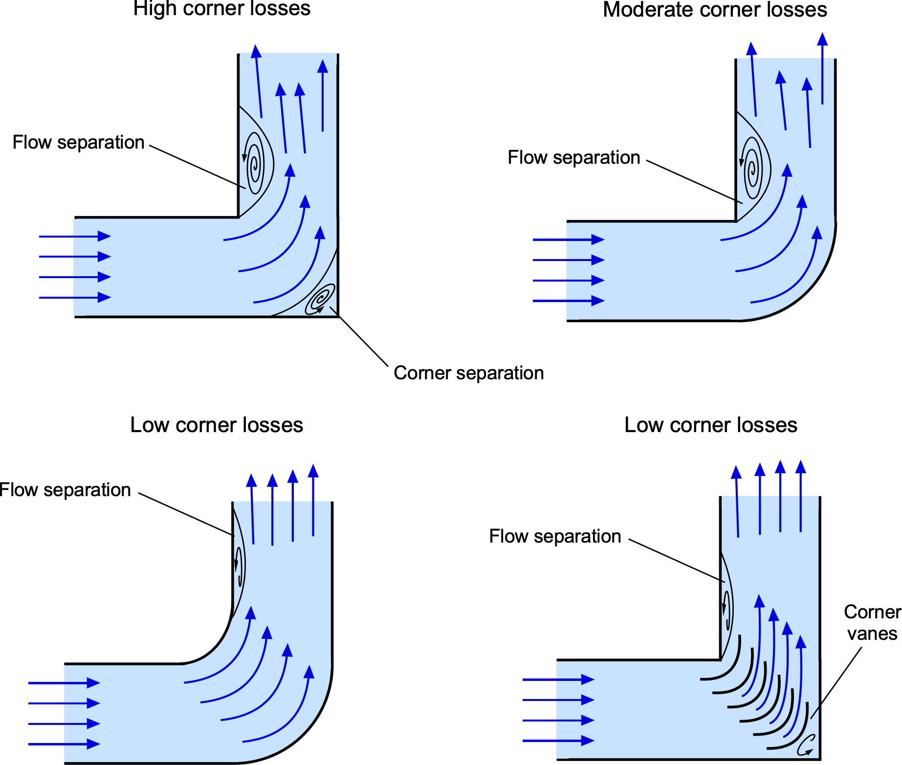
The magnitude of the pressure drop around a corner depends on various factors, such as the geometry of the bend, flow rate, fluid viscosity, and Reynolds number. Many studies have been to determine the losses in bends, including by NIST. One way of assessing such pressure losses is by using a local loss coefficient  , for which values are published for various corners and bends. The local pressure loss, , is given by
(54) 
where is the head loss. The head loss is then
(55) 
which is often referred to as a velocity head. For a sharp corner,  , as shown in the figure above, and for a smooth corner,
  .
.
Many hydraulic, pneumatic, and other internal fluid flow systems comprise straight sections, turns, and branches. The total pressure losses are the sum of all of the pressure losses incurred by each component of the system, i.e.,
(56) 
Today, computational fluid dynamics (CFD) can better predict and analyze the specific pressure drop for a given internal flow system. In general, the pressure drop around a corner can be minimized by using smooth bends with large radii, which limit the possibilities of flow separation. Additionally, properly designed flow control devices, such as corner vanes or deflectors, can limit the pressure drop.
Wind Tunnels
Wind tunnels are critical tools for simulating and analyzing airflow over aircraft, vehicles, buildings, and other structures. They are central to the aerospace design process, providing engineers with essential data that cannot be fully predicted before flight. Wind tunnel testing builds confidence that an aircraft will perform as intended. Proper tunnel design, which is based on internal flow principles, ensures reliable, repeatable measurements and enables their use across many fields beyond aerospace. Although wind tunnels vary widely in size and speed capabilities, their core function is to produce controlled flow environments for experimental measurements. Tests are typically performed on scale models, wings, and other components. Achieving dynamic similarity with full-scale conditions often requires careful geometric and flow parameter scaling. However, because wind tunnel models are sub-scale, matching both Reynolds and Mach numbers simultaneously remains a fundamental challenge.
Fundamental Components of a Wind Tunnel
A wind tunnel typically comprises five key sections, each with a specific function that contributes to the overall performance and accuracy of the system. A schematic of a ERAU wind tunnel is shown below. This is a closed-return wind tunnel with a 4 ft by 6 ft (1.22 m by 1.83 m) rectangular test section 12 ft (3.66 m) long with tapered corner fillets. This tunnel allows flow speeds of up to 420 ft/s (128 m/s, 460 km/h, 286 mph) to be obtained in the test section with exceptional flow quality and low turbulence levels. In addition, the test section has about 65% of its surface area made with optical grade glass, allowing flow measurements using optical methods such as particle image velocimetry (called “PIV”).
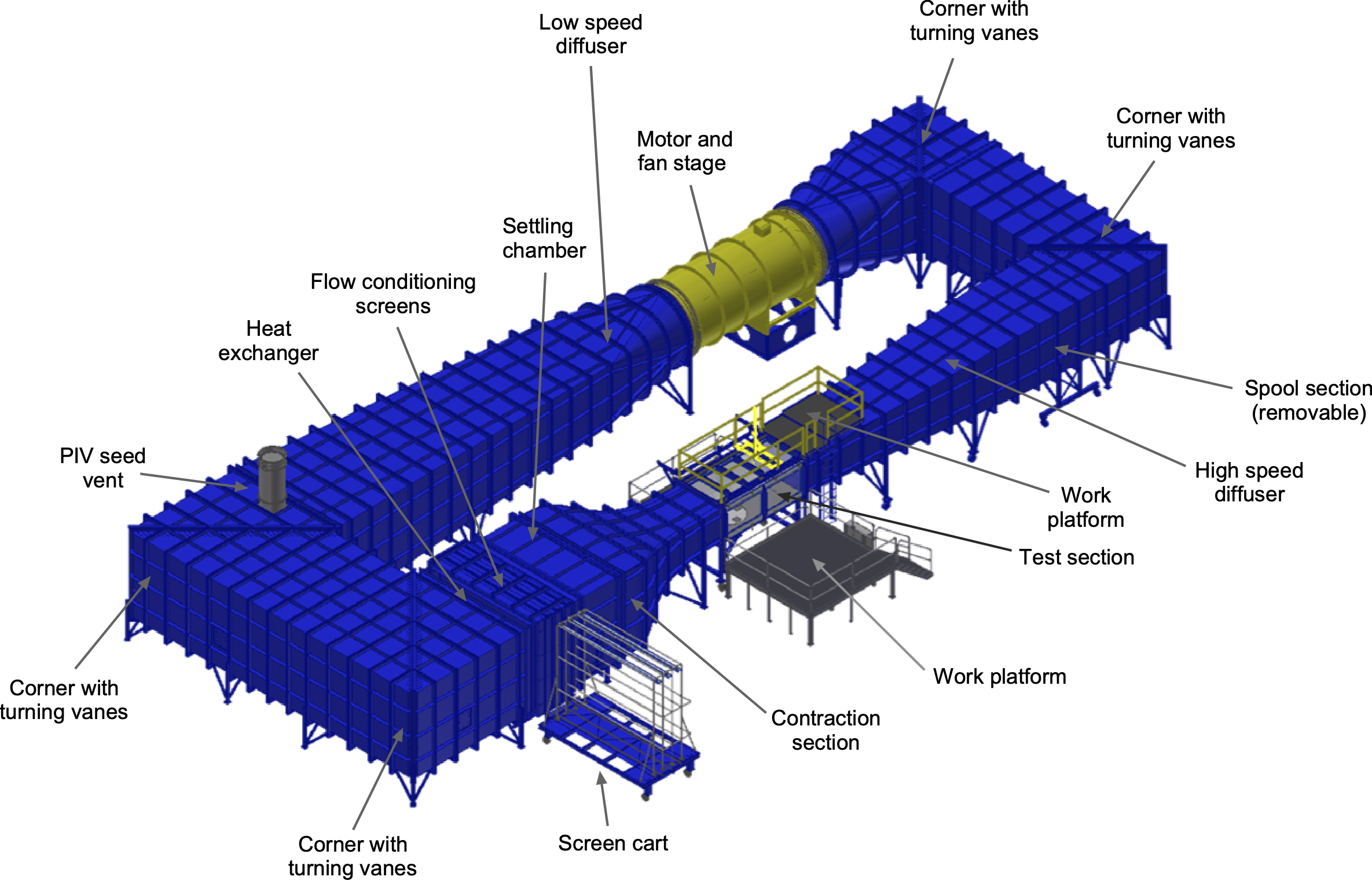
The settling chamber, located at the entrance of the tunnel, conditions the incoming air and reduces turbulence using flow straighteners, typically honeycomb structures and mesh screens, which remove swirl and ensure a uniform velocity profile before contraction. In closed-return tunnels, this section may also house heat exchangers to control air temperature. The contraction section then accelerates the flow smoothly into the test section, often using a parabolic or exponential profile. In addition to increasing velocity, this section further damps out turbulence through a squeezing effect on the remaining eddies. The test section is the core of the wind tunnel, where models are placed and measurements are made. It is designed to ensure uniform flow with minimal boundary layer influence and includes transparent walls for optical diagnostics and ports for instrumentation. Following this, the diffuser decelerates the airflow to recover pressure while avoiding separation. A well-designed diffuser with a shallow diffuser angle is essential to maintaining tunnel efficiency. Finally, the drive section contains the fan or blower that powers the tunnel. High-performance fans may feature variable speed control and adjustable pitch blades.
Pressure Losses in Wind Tunnels
One key challenge in wind tunnel design is determining the required fan or motor power to generate a desired test-section velocity or dynamic pressure. This depends on accurately estimating pressure losses throughout the tunnel circuit. Because wind tunnels contain ducts of varying shapes, areas, and transition pieces, flow moving through them experiences friction and other losses, particularly at higher Reynolds numbers. Additional pressure losses arise from turning vanes placed at circuit corners, typically cascades of thin airfoil-shaped plates, which help redirect flow but introduce substantial resistance. Careful estimation of these cumulative losses is essential to ensure the tunnel meets its performance targets.
In the conventional approach to wind tunnel design, the frictional losses can be estimated for the fan and initial sizing of the motor by breaking the tunnel circuit into its primary parts:
- Cylindrical sections (even if just transition pieces).
- Corners.
- Expanding sections, i.e., diffusers.
- Contracting sections, i.e., nozzles.
- Turbulence screens.
- Heat exchangers.
- Other miscellaneous parts.
In each of these sections (and there may be more than one of each), energy is lost in the form of a static pressure drop , which can be expressed as a dimensionless local loss coefficient
(57) 
where  is the local dynamic pressure. For corners, bends, and turning vanes, the loss coefficient is typically based on empirical data, as previously discussed. This loss is referenced to the test section values (subscript 0) using
(58) 
Although Poiseuille’s law applies to fully developed laminar flow and is not directly applicable to the high-Reynolds-number, turbulent flows in wind tunnels, a similar scaling relationship can still be used to approximate geometric effects. Specifically, for ducts of varying cross-sections, pressure loss coefficients can be scaled based on the fourth power of the hydraulic diameter
(59) 
where is the local hydraulic diameter of the tunnel section, and  is the hydraulic diameter of the test section. The hydraulic diameter is defined as
(60) 
where  is the cross-sectional area and is the wetted perimeter of the section.
The next step is to express the energy loss per unit time,  , in terms of the test section conditions, i.e.,
(61) 
which simplifies to
(62) 
The so-called energy ratio,  , can then be defined as
(63) 
so that
(64) 
This formulation shows that minimizing  , including corner losses through the values of , improves the tunnel’s efficiency and reduces the power required by the fan.
The energy ratio, , represents the efficiency of a wind tunnel circuit and is inversely related to the total energy losses in the system. For a well-designed closed-return tunnel, typically ranges from 4 to 7. Lower pressure losses mean greater efficiency and lower power demand from the fan and motor. Major losses often arise in diffuser sections and corner vanes, making their design critical. Calculating the loss coefficients ( ) for each section involves applying standard aerodynamic relationships for turbulent flow through ducts, fittings, vanes, turbulence screens, and other elements. Losses within the fan or motor are generally excluded from to isolate the tunnel design efficiency. Estimating these losses is necessary to determine the fan power required, called the pumping power, to achieve the target test-section velocity. Because some losses can only be approximated before construction, wind tunnel designs typically include some power margins to ensure that the specifications are met.
Check Your Understanding #4 – Calculating the power required to drive a low-speed wind tunnel
Estimate the minimum motor power required for a low-speed wind tunnel with a maximum flow speed of 230 mph in the test section. The test section area is 22.5 ft, and the energy ratio of for the tunnel is 5.2. The fan efficiency is 0.74%, and the motor efficiency is 90%.
The specification of the energy ratio gives the cumulative losses in the tunnel, so the first step is to find the energy of the flow in the test section, i.e.,
![\[ \mbox{\small Energy} = \frac{1}{2} \varrho \, A_0 \, V_0^3 \]](https://eaglepubs.erau.edu/app/uploads/quicklatex/quicklatex.com-2444e17b5442a5fb50c530c718ebf0d9_l3.svg "Rendered by QuickLaTeX.com")
The value of  is 22.5 ft and
  = 230 mph = 337.33 ft/s. Assume MSL ISA for the air density, so = 0.002378 slug ft
 . This gives
![\[ \mbox{\small Energy} = \frac{1}{2} \varrho \, A_0 \, V_0^3 = 0.5 (0.002378) (22.5) (337.33)^3 = 1.0269 \times 10^6 \]](https://eaglepubs.erau.edu/app/uploads/quicklatex/quicklatex.com-8e14d97bd8e0ef64d16396bcf7409f63_l3.svg "Rendered by QuickLaTeX.com")
Therefore, the power required to be delivered to the air at the fan/motor stage would be
![\[ P_{\rm air~power} = \frac{\mbox{\small Energy (at test section)} }{ER_t} = \frac{1.0269 \times 10^6 }{5.2 \times 550} = 359.1~\mbox{ hp} \]](https://eaglepubs.erau.edu/app/uploads/quicklatex/quicklatex.com-ccf158dff25e13470a0f564cec4ff192_l3.svg "Rendered by QuickLaTeX.com")
Taking into account the fan and motor efficiency then, the minimum power required would be
![\[ P_{\rm req} = \frac{P_{\rm air~power}}{\eta_p \, \eta_m} = \frac{359.1}{(0.74)(0.90)} = 539.1~\mbox{ hp} \]](https://eaglepubs.erau.edu/app/uploads/quicklatex/quicklatex.com-3be5284e28f56b5abef7ec09248d7c28_l3.svg "Rendered by QuickLaTeX.com")
This latter result would only be valid for an empty test section, and to get the same flow speed with an article in the test section, more power would be needed to overcome the drag and “blockage'” of the article. This value is generally unknown a priori. However, it is usually considered reasonable to add a margin of power to overcome a winged test article with a wing span of 0.8 of the tunnel diameter (or width), an aspect ratio of 5, and a  of 1.0. Furthermore, to account for the potential diversity of test articles (not all will be streamlined shapes), a margin of 50% more power may be needed. The final estimated rated motor power for the tunnel would be about 900 to 1,000 hp.
Summary & Closure
Internal flows are encountered in various aerospace applications, such as engine air intakes, fuel systems, hydraulic systems, air conditioning systems, wind tunnels, and other applications where fluids flow through pipes and ducts. A significant consideration for internal flows is that frictional effects from the action of viscosity produce significant pressure drops along the length of the pipe or duct. These pressure drops require a source of power to pump the fluid along the pipe or duct, and this power required is related to the flow velocity and internal surface finish. Because such flows are inevitably turbulent, a Moody chart must be used to determine the friction factors and estimate the resulting pressure drops for design purposes. Internal flows are critical within the combustion chambers of jet and rocket engines, where combustion produces high-temperature, high-pressure gases to produce thrust. Aircraft and spacecraft have environmental control systems to maintain comfortable conditions for passengers and crew, which also require the analysis of internal flows. Understanding and optimizing internal flows in aerospace applications are essential for improving efficiency, safety, and overall performance.
5-Question Self-Assessment Quickquiz
For Further Thought or Discussion
- For an aircraft’s hydraulic system, discuss some potential design trades in operating the hydraulic system with smaller pipes and higher pressure versus larger pipes and lower pressure.
- What is the definition of internal flow in fluid dynamics? How does internal flow differ from external flow, and what are some examples of each?
- Consider the fuel and oxidizer system for a rocket engine, which requires high mass flow rates of cryogenic liquids. What are the internal flow issues to consider regarding the delivery of the fuel and oxidizer to the combustion chamber in this case?
- The corner or turning vanes in a wind tunnel are a large source of losses. Consider the engineering steps you might take to calculate and minimize such losses.
- Explain the significance of the Reynolds number in internal flows. How does it affect the flow characteristics? Compare the flow regimes associated with low and high Reynolds numbers in internal flows.
- Explain the major differences between flow in circular pipes and non-circular conduits. How do these differences impact flow characteristics?
Other Useful Online Resources
To learn more about internal flows, take a look at some of these online resources:
- A film that discusses the use of the wind tunnel: The Secret of Flight 1: Preview.
- Web site on internal flows from Wikiversity.
- Fluid dynamics review on internal flows.
- A video lecture on internal flows and entrance length.
- ANSYS course video on losses is pipes and ducts.
- See here and here for video lectures on how to use a Moody chart.
- A handy online calculator for friction factors using the Moody chart.
- See: "The History of Poiseuille's Law," by S. P. Sutera and R. Skalak, Annual Review of Fluid Mechanics, Volume 25, 1993. According to them, the naming of Equation 36 as Poiseuille's law occurs in a publication by Hagenbach (1860), who, after giving the derivation, generously suggested calling it Poiseuille's law. Jacobson (1860) also refers to Equation 36 as Poiseuille's law. See: Hagenbach, E. 1860, "Uber die Bestimmung der Zahigkeit einer Fliissigkeit durch den Ausfluss aus R6hren," Poggendorf's Annalen der Physik und Chemie, Vol. 108, pp. 38–426, and Jacobson, H. 1860, "Beitriige zur Haemo dynamik," Archives of Anatomy and Physiology, Vol. 80, pp. 80–113. ↵
