Flight Maneuvers & Gusts

J. Gordon Leishman

doi:https://doi.org/10.15394/eaglepub.2022.1066.n39

46 Flight Maneuvers & Gusts

Introduction

To design and engineer an aircraft, it is necessary to know what it is expected to do regarding its flight characteristics, including its maneuver performance. All aircraft types must be able to maneuver to some degree, some more than others. Airliners, for example, are only expected to perform gentle maneuvers, such as shallow climbs and descents, and moderate banked turns. Examples of more extreme flight maneuvers are high-rate turns, rapid pull-ups, and various aerobatics, as shown by the airplanes in the photograph below, or any situation where an aircraft may follow a curvilinear path under non-steady, accelerated flight conditions.

A flight team performs formation aerobatic maneuvers.

However, any flight maneuver will have some limits, and an aircraft’s actual maneuver performance will be constrained by its aerodynamic capabilities and the structural strength of its airframe. For example, the ability to perform various high load factors or high “ $g$ ” maneuvers is expected of many military airplanes, especially jet fighters. Therefore, not only must the airframe be sufficiently strong to carry the loads in these maneuvers, but the airplane’s aerodynamic performance must be carefully considered in that aerodynamics is not a prematurely limiting factor. In this regard, the desired maneuver capability must not be limited too early by the onset of wing stall and/or buffeting.

Natural gusts in the atmosphere will also cause loads on the airplane that are over and above those produced in steady, level flight in smooth air. In particular, vertical gusts can produce transient loads on an airplane that may be as large, or even more significant, than those expected during maneuvers and those that are otherwise within the standard flight envelope. For this reason, the airplane’s needed maneuver performance and gust loading capabilities must be precisely defined, and the aerodynamics and structural requirements must be carefully established during the design process. Naturally, these capabilities also need to be verified by structural testing, which will be undertaken using a systematic combination of flight and ground tests.

Learning Objectives

Understand the meaning and significance of the airspeed/load factor or “ $V$ – $n$ ” diagram for maneuvers and atmospheric gusts.
Be able to interpret the $V$ – $n$ diagram and identify critical airspeeds.
Appreciate why the airspeed at which wing stall occurs will increase during a maneuver or when a load factor is applied.

Equations of Motion

As previously derived, the following general equations can be used to describe the motion of an airplane, i.e.,

(1) $\begin{eqnarray*} \mbox{$\parallel$ to flight path:} \quad && \hspace*{-7mm} \left(\frac{W}{g}\right) \frac{d V_{\infty}}{dt} = T \cos \epsilon - D - W \sin \theta \\[10pt] \mbox{$\perp$ to flight path:} \quad && \hspace*{-7mm} \left(\frac{W}{g}\right) \frac{V_{\infty}^2}{R} = L \cos \phi + T \sin \epsilon \cos \phi - W \cos \theta \\[10pt] \mbox{Horizontal plane:} \quad && \hspace*{-7mm} \left(\frac{W}{g}\right) \frac{(V_{\infty} \cos \theta)^2}{R} = L \sin \phi + T \sin \epsilon \sin \phi \end{eqnarray*}$

The angle $\theta$ can be viewed as the climb or flight path angle, and the bank angle is denoted by $\phi$ . It should be remembered that during maneuvers, which are accelerated flight conditions, the lift on the wing will not equal the weight of the airplane because of the need for the wing to create whatever lift value is needed to produce the necessary accelerations to follow the required flight path. This lift force may be greater or less than the airplane’s weight, so during flight, the load factor can be positive (i.e., an upward acceleration) or negative (downward acceleration).

In many cases, the line of action of the thrust vector relative to the flight path is small, so it is reasonable to assume that $\epsilon = 0$ in the forgoing equations, i.e.,

(2) $\begin{eqnarray*} \mbox{$\parallel$ to flight path:} \quad && \hspace*{-7mm} \left(\frac{W}{g}\right) \frac{d V_{\infty}}{dt} = T - D - W \sin \theta \\[10pt] \mbox{$\perp$ to flight path:} \quad && \hspace*{-7mm} \left(\frac{W}{g}\right) \frac{V_{\infty}^2}{R} = L \cos \phi - W \cos \theta \\[10pt] \mbox{Horizontal plane:} \quad && \hspace*{-7mm} \left(\frac{W}{g}\right) \frac{(V_{\infty} \cos \theta)^2}{R} = L \sin \phi \end{eqnarray*}$

Maneuvers in a Vertical Plane

Consider first the forces on an airplane maneuvering in a vertical plane with wings level ( $\phi$ = 0) following a circular flight path of instantaneous radius $R$ and at a constant airspeed $V_{\infty}$ , as shown in the figure below. Notice that the airplane would perform a complete loop in a vertical plane when continuing this trajectory.

The balance of forces on an airplane in a pull-up maneuver.

The airplane’s mass is $M (= W/g$ ), so $W \cos \psi$ is the vertical component of the weight. Vertical equilibrium in the maneuver requires that

(3) $\begin{equation*} L - W = \left( \frac{W}{g} \right) \frac{V_{\infty}^2}{R} \end{equation*}$

Therefore, the lift required on the wing to follow the flight path is

(4) $\begin{equation*} L = \left( \frac{W}{g} \right) \frac{V_{\infty}^2}{R} + W = \left( 1 + \frac{V_{\infty}^2}{g R} \right) W = n \, W \end{equation*}$

i.e., the lift must be greater than the weight, where the load factor $n$ is

(5) $\begin{equation*} n = \left( 1 + \frac{V_{\infty}^2}{g R} \right) \end{equation*}$

The excess lift is related to the load factor, $n$ , such that $L = n \, W$ , i.e., the number of effective “ $g$ ‘s.” So, it can be seen that for a given radius of the flight path, the load factor increases with the square of the airspeed. Furthermore, for a given airspeed, the load factor is inversely proportional to the radius, i.e., a faster and/or tighter flight path will produce a higher load factor. The radius of curvature $R$ of the flight path, in this case, will be

(6) $\begin{equation*} R = \frac{V_{\infty}^2}{g (n - 1)} \end{equation*}$

so for a given load factor, the radius of the flight path increases quickly with the square of the airspeed.

Looping Maneuver

Continuing the pull-up will result in a looping type of maneuver. It is unlikely that a commercial airliner will perform loops, as might be suggested in the figure, but the point of the trajectory is made. As previously discussed, lift on the wing must be sufficient to overcome the airplane’s weight and produce the centripetal acceleration to execute a circular flight path in a vertical plane. The angular position of the airplane in the flight path must also be considered. The lift required in a loop is needed to overcome the component of the weight acting on the airplane at any given angle $\psi$ , plus the necessary centripetal force, i.e.,

(7) $\begin{equation*} L = \underbrace{ \left( \frac{W}{g} \right) \frac{V_{\infty}^2}{R_v}}_{\begin{tabular}{c} \scriptsize Centripetal \\[-3pt] \scriptsize force \end{tabular}} + \underbrace{W \cos \psi}_{\begin{tabular}{c} \scriptsize Component \\[-3pt] \scriptsize of weight \end{tabular}} = \underbrace{ \left(\frac{V_{\infty}^2}{g \, R} + \cos \psi \right)}_{\begin{tabular}{c} \scriptsize Load factor \end{tabular}} W = n W \end{equation*}$

where $\psi = 0^{\circ}$ when the airplane is at the bottom of the loop, as shown in the figure below. Notice that weight always acts vertically downward. It can be assumed that the thrust is modulated by the pilot to keep the airplane at a constant airspeed.

The balance of forces on an airplane in a looping type of flight maneuver with wings level in a vertical plane.

The corresponding load factor will be

(8) $\begin{equation*} n = \left( \cos\psi + \frac{V_{\infty}^2}{g \, R_v} \right) \end{equation*}$

At the bottom of the loop where $\psi = 0^{\circ}$ , the lift must be greater than the weight to overcome both the weight and create the needed centrifugal force so

(9) $\begin{equation*} n = \left(1 + \frac{V_{\infty}^2}{g \, R_v} \right) \end{equation*}$

At the top of the loop where $\psi = 180^{\circ}$ , the weight helps in the direction of the centripetal force, so the load factor is

(10) $\begin{equation*} n = \left(-1 + \frac{V_{\infty}^2}{g \, R_v} \right) \end{equation*}$

and so this is less than at the bottom of the loop. Notice that the load factor is a function of airspeed $V_{\infty}$ and the radius of the loop $R_v$ . If the pilot flies a loop at a higher airspeed or tightens the loop to get a smaller radius $R_v$ , the pilot will experience higher load factors.

Consider now a flight maneuver where an aerobatic airplane is inverted at the top of a perfectly circular loop performed at a constant airspeed, with the pilot modulating the engine thrust or power accordingly. Consider the case where the combination of airspeed and flight path radius gives

(11) $\begin{equation*} \frac{V_{\infty}^2}{g \, R_v} = 1 \end{equation*}$

Balance of forces during a “loop-the-loop” maneuver.

The lift required is

(12) $\begin{equation*} L = \left( \frac{W}{g} \right) \frac{V_{\infty}^2}{R_v} + Mg \cos \psi = \left( 1 + \frac{V_{\infty}^2}{g \, R_v} \right) W = n W \end{equation*}$

The corresponding load factor will be

(13) $\begin{equation*} n = \left( \cos\psi + \frac{V_{\infty}^2}{g \, R_v} \right) \end{equation*}$

At the bottom of the loop, the lift must be greater than the weight to overcome both the weight and create the centrifugal force so that the load factor will be

(14) $\begin{equation*} n = \left(1 + \frac{V_{\infty}^2}{g \, R_v} \right) \end{equation*}$

At the top of the loop, the weight helps in the direction of the centrifugal force, so the load factor here is

(15) $\begin{equation*} n = \left(-1 + \frac{V_{\infty}^2}{g \, R_v} \right) \end{equation*}$

so it will be less than at the bottom of the loop. In this case, where

(16) $\begin{equation*} \frac{V_{\infty}^2}{g \, R_v} = 1 \end{equation*}$

then the pilot will feel “weightless,” i.e., $n = 0$ .

Notice that for a given load factor, the radius of the flight path increases quickly with the square of the airspeed. This result explains the development of tactics needed for combat maneuvers used by military airplanes, where tighter maneuvers must often be performed at lower airspeeds. The corresponding angular rate in the maneuver is

(17) $\begin{equation*} \omega = \frac{d\gamma}{dt} = \frac{g (n - 1)}{V_{\infty}} \end{equation*}$

which again confirms that tighter maneuvers are best flown at lower airspeeds.

Zero-g Flight Maneuvers

Zero-g maneuvers in an airplane can be used to simulate the weightlessness of space. One airplane used for this purpose was the “Weightless Wonder,” operated by NASA, also known as a “Reduced Gravity Aircraft.” In a parabolic “zero-g” flight, the airplane follows a specific flight trajectory that creates several seconds of weightlessness for the occupants inside. To conduct this maneuver, the airplane must have a minimum entry speed, which defines the initial kinetic energy state needed to complete the maneuver without the wing stalling; the airspeed to fly will depend on the specific airplane, its in-flight weight, and the number of occupants.

The pilots first initiate a steep pull-up climb, and the pitch attitude may approach 45 degrees. The pilots will then “push over” to lower the nose of the airplane to maintain whatever pitch attitude and angle of attack (and lift on the airplane) that is necessary to balance the outward radial centrifugal force against the force of gravity (i.e., weight), as shown in the figure below. When the outward centrifugal and residual lift forces balance the airplane’s weight, the net force that is normal to the airplane’s trajectory will be zero. Therefore, the occupants will experience a period where the load factor $n \approx 0$ or “zero-g,” during which they will feel “weightless.” It is a pleasant experience, although the conditions leading up to and after may not be.

When the outward centrifugal force and residual lift force balance weight, the occupants will experience a period of “zero-g,” during which they feel “weightless,” thereby simulating the conditions in space.

At the apogee of the “zero-g” parabolic (nominally) trajectory then, the equation of force equilibrium is

(18) $\begin{equation*} L + \frac{V_{\infty}^2}{g \, R_v} - M \, g = n \, M \, g + \frac{V_{\infty}^2}{g \, R_v} - M \, g = ( n - 1) M \, g + \frac{V_{\infty}^2}{g \, R_v} = 0 \end{equation*}$

Therefore, for $n = 0$ , i.e., weightless, then

(19) $\begin{equation*} \frac{V_{\infty}^2}{g \, R_v} = M \, g = W \end{equation*}$

which will give the combination of airspeeds, $V_{\infty}$ , and radii of curvature of the flight path, $R_v$ , for the weightless condition at a given flight weight, $W$ . If, for example, the radius of curvature of the flight path is held constant, then the airspeed to fly for the zero-g condition is

(20) $\begin{equation*} V_{\infty} = \sqrt{ M \, g^2 \, R_v } = \sqrt{ W \, g \, R_v } \end{equation*}$

Maintaining a constant airspeed is critical. As the nose of the airplane is pitched up, airspeed will bleed off quickly, so it requires the addition of engine thrust. After the apogee, the airplane will continue in an increasingly nose-down pitch attitude with increasing airspeed, so thrust must be reduced. Using airbrakes and/or spoilers will help maintain airspeed and the zero-g conditions for a few more seconds, after which recovery must be initiated by pulling back on the controls and applying thrust. These unique “zero-g” conditions, albeit only lasting between 10 and 20 seconds, allow engineers and astronauts to experience the conditions of weightlessness without going to space and so prepare for actual space flights.

The repeated cycles of ascent and descent during the “zero-g” flights are like a roller-coaster-like experience, which can be uncomfortable for the occupants and even the most seasoned pilots, especially after twenty or more contiguous trajectories. The sensation of weightlessness can also lead to motion sickness for some individuals, the airplane being used for these “zero-g” flights earning the nickname “Vomit Comet.” The disorientation that humans feel between inner ear responses and balance and visual cues from the eye during weightless conditions, produce neurotoxic responses and symptoms of dizziness and even disorientation that astronauts call “space sickness.” No human is immune; even test pilots and astronauts may need to take motion-sickness medications.

Maneuvers in a Horizontal Plane

Now consider the forces on an airplane in a pure horizontal turn with a bank angle $\phi$ and when flying at a constant airspeed $V_{\infty}$ , as shown in the figure below.

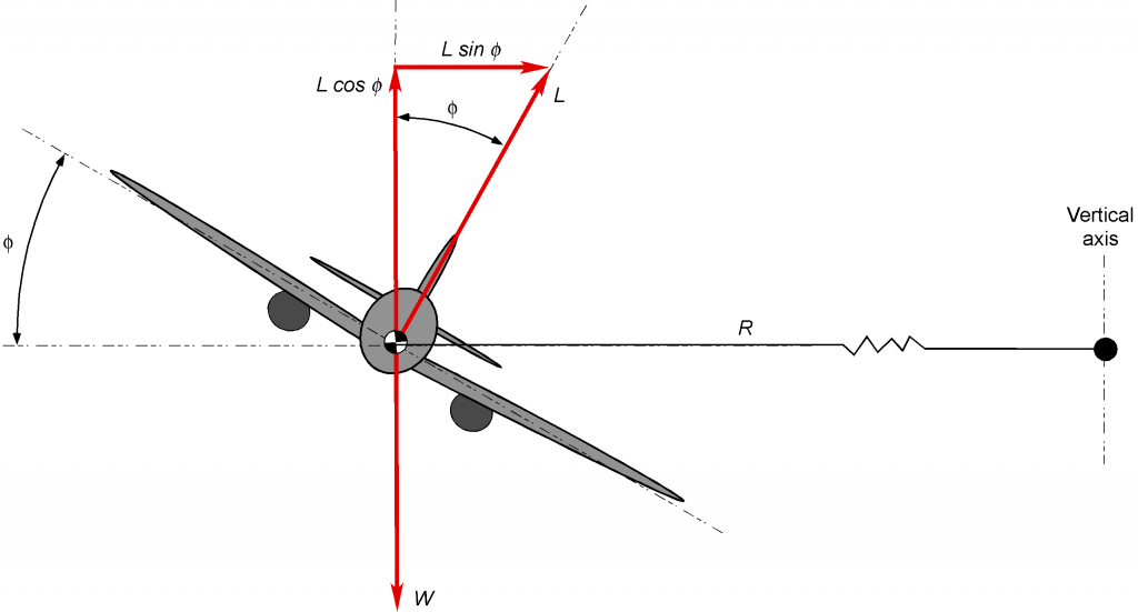
The balance of forces on an airplane in a turning maneuver.

Vertical equilibrium requires that

(21) $\begin{equation*} L \cos \phi = W \end{equation*}$

and horizontal equilibrium requires

(22) $\begin{equation*} L \sin \phi = \left(\frac{W}{g} \right) \frac{V_{\infty}^2}{R} \end{equation*}$

where $R$ is the instantaneous radius of curvature of the turn.

It is apparent then that to perform a turn, the lift on the wing must again be greater than the weight of the airplane, i.e., $L > W$ , to create the necessary aerodynamic force not only to balance the weight of the airplane but also to produce the inward radial force to create the needed centripetal acceleration to execute the turn.

Solving for the lift required gives

(23) $\begin{equation*} L = \frac{W}{\cos \phi} \end{equation*}$

and so the load factor is

(24) $\begin{equation*} n = \frac{W }{W \cos \phi} = \frac{1}{\cos \phi} \end{equation*}$

The preceding result shows that the load factor must increase with the inverse of the cosine of the bank angle $\phi$ . For example, a 60 $^{\circ}$ banked turn will correspond to $n = 2$ , i.e., a load factor of two.

Airspeed-Load Factor Diagram

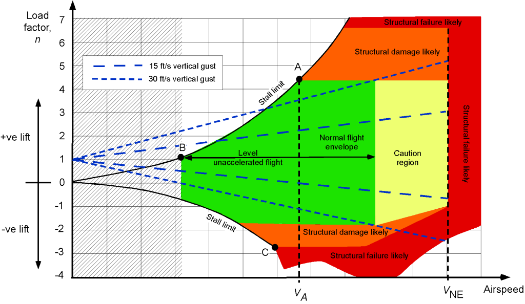
An airspeed-load factor or $V$ – $n$ diagram is one form of operating envelope for an airplane. The figure below shows a representative $V$ – $n$ diagram for an airplane as a function of indicated airspeed. However, equivalent airspeed (related to actual dynamic pressure) or Mach number will sometimes be used on the “airspeed” axis.

Representative maneuver envelope for an airplane in terms of load factor versus airspeed. Each type of airplane will have its specific envelope.

Aerodynamic Limits

As previously discussed, airplanes will be limited aerodynamically by the onset of stall and/or buffet. The stall speed with a steady load factor $n$ is

(25) $\begin{equation*} V_{s_{ng}} = \sqrt{\frac{ 2 n W}{\varrho_{\infty} S C_{L_{\rm max}}}} = \sqrt{n} \, V_{s_{1g}} \end{equation*}$

This latter result shows that the airplane will stall at a higher airspeed when pulling any “ $g$ ” loading with $n > 1$ . Notice from the $V$ – $n$ diagram that as the load factor increases, the stall airspeed follows a curve defined by Eq. 25, i.e., its value increases, and so it traces out one part of the envelope on the $V$ – $n$ diagram.

Structural Limits

The $V$ – $n$ diagram also reflects that an airplane can only structurally withstand a finite amount of loading (e.g., it is capable of only so much wing stress and/or wing bending and/or skin. buckling) until it suffers permanent damage or structural failure; this maximum loading is denoted by $n_{\rm max}$ . At one airspeed, which is called the corner airspeed or the maximum maneuvering airspeed, the airplane will be operating at the edge of the stall and pulling the maximum load factor, i.e.,

(26) $\begin{equation*} V_A = \sqrt{\frac{ 2 n_{\rm max} \, W}{\varrho_{\infty} \, S \, C_{L_{\rm max}}}} \end{equation*}$

The maximum maneuvering airspeed is often called $V_A$ (or sometimes $V_a$ ).

Equation 26 defines an aerodynamic limitation on overall flight performance because of the attainment of the maximum lift coefficient $C_{L_{\rm max}}$ on the wing, as well as a structural limitation in terms of a maximum attainable structural load factor. Therefore, for flight in rough air other than light turbulence or “chop,” the pilot or aircrew must operate the airplane at its maximum maneuvering equivalent airspeed $V_A$ , which is marked on the airspeed indicator (white arc). This approach is required so that unexpected turbulent gusts will not create load factors that could potentially overload the airframe.

The maximum attainable load factor $n_{\rm max}$ that an airplane is designed to withstand, i.e., its structural limits, depends on the airplane type and what it is intended to do. For civil airplanes, the limiting values of the load factor will be defined by the appropriate certification authority, e.g., by the FARs in the U.S. Under limit load conditions, the FARs require that the airplane’s structural components support those loads without any permanent detrimental structural deformations and that the stresses remain below the critical yield point to account for unexpected events such as severe gust loads. Another consideration is something like an emergency landing at weights that are higher than the standard landing weights.

Normal Category Airplanes

For transport category airplanes (e.g., airliners), $n_{\rm max}$ ranges from $-1 g$ to $+2.5 g$ or up to $+3.8 g$ , depending on the design takeoff weight. To the limit load factors, a value of 50% is added for structural design purposes (i.e., an extra margin for extra safety), i.e., the ultimate structural strength needs to be at least 150% of the design limit load, which then becomes known as the ultimate load.

For normal and commuter category airplanes, limit load factors range from $-1.52 g$ to $+3.8 g$ . The maximum specified load factor is only $2.5 g$ for airplanes with a gross weight of less than 50,000 lb but increases linearly with weight up to a maximum of $3.8 g$ . The relevant equation the FARs defines is $n = 2.1 + 24,000/(W +10,000)$ up to a maximum of $3.8 g$ where $W$ is measured in lb. For utility category airplanes (or those configured to operate in this category) range from $-1.76 g$ to $+4.4 g$ , which often allows the airplanes to perform limited aerobatics, at least within a specific center of gravity range.

Aerobatic Airplanes

The load factor ranges from $-3.0 g$ to $+6.0 g$ for fully acrobatic or aerobatic category airplanes. However, in particular for aerobatic and military fighter airplanes, many airplane types are designed to tolerate load factors much higher than the minimum required by regulations, often between $-10 g$ and $+12 g$ . Aerobatic airplanes are generally much stronger than the pilot could sustain in terms of “ $g$ ” loadings.

The following additional points identify and describe the nature of the $V$ – $n$ diagram and what it means:

Strictly speaking, the $V$ – $n$ diagram applies to a single flight weight. Usually, a $V$ – $n$ diagram is defined at the maximum gross in-flight weight of the airplane, i.e., $W_{\rm GTOW}$ .
The area inside the “Normal flight envelope,” as marked out by the $V$ – $n$ diagram, is the combination of airspeeds and load factors where the airplane can be safely flown without stalling or suffering structural failure.
At a load factor unity ( $n = 1$ ), which is level flight, the stall limit can be easily identified on the $V$ – $n$ diagram.
The corner airspeed where the airplane is operating at the edge of the stall and pulling the maximum load factor can be easily identified. This point is usually marked on the diagram as the maximum maneuvering airspeed or $V_A$ (an equivalent airspeed and the limit of the “white arc” on the airspeed indicator).
Notice that both positive and negative load limits are identified. The airplane usually cannot withstand as much negative loading as positive loadings, as will the pilot and passengers. The exception, of course, is an airplane designed specifically for aerobatics.

Limiting Airspeeds

At higher airspeeds, the airplane reaches an aerodynamic limit based on dynamic pressure, i.e., this represents a “redline” or never-exceed airspeed, and is usually identified as $V_{\rm NE}$ and marked on the pilot’s airspeed indicator. Structural failure can be expected if exceeded, even by some narrow margin. Therefore, a “yellow arc” zone will also be marked on the airspeed indicator so the pilot knows that the airplane is operating near its maximum airloads and structural capability.

Structural Testing

A new airplane design’s limit and ultimate failure loads (and its components) are validated on the ground. To this end, a test article of the entire airplane is mounted in a special rig that can simulate the magnitude and distribution of the airloads encountered during the actual flight, as shown in the photograph below. Naturally, this sort of test to failure would not be done in the air! The airplane will be randomly selected “as built” on the regular production line, so no special considerations are given to the airplane’s structure.

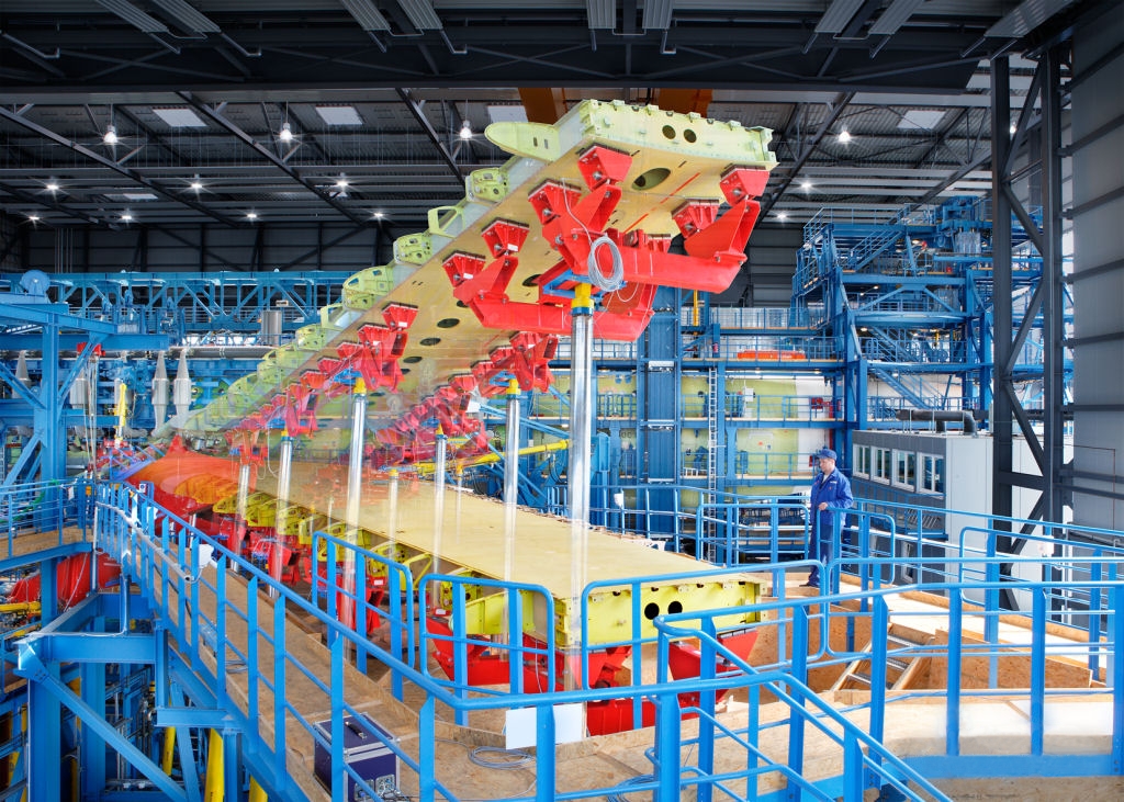
Structural tests on the ground can verify the ultimate load factor of a wing.

Other tests performed in this type of ground rig include simulations of extreme negative loads on the wing to validate the lower part of the $V$ – $n$ diagram, maneuver loads, and emergency landing loads. For a military airplane, ballistic damage to the wing may also be a consideration, i.e., various types of damage may result in structural stress and a loading limitation. Eventually, the wing will be tested to destruction to verify the predicted ultimate loads on the airplane can indeed be sustained. In most cases, wings will fail by compression buckling of the upper wing skins.

Gust-Induced Airloads

There are two primary uses for a $V$ – $n$ diagram, one for maneuvering flight, as already considered, and another for the gust loads in the atmosphere produced when flying along in straight-and-level flight. The diagrams are basically the same, but the presented information has different interpretations. The atmosphere is never stagnant, and turbulence and gusts occur naturally. A gust can affect the airplane from any direction. However, upward (vertical) gusts, as shown in the figure below, have the most pronounced effects on the airplane regarding aerodynamic response and induced load factor.

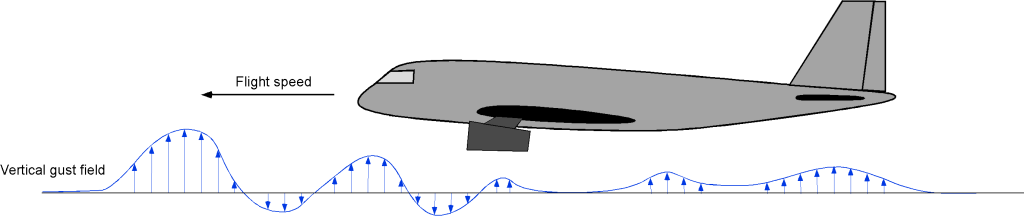
While gusts in the atmosphere can be produced from any direction, vertical gusts will have the most pronounced aerodynamic effects on the airplane.

The primary effect of a vertical gust is to increase the wing’s angle of attack and, thus, the wing lift, as shown in the figure below. While there will also be an effect on drag, the effects are minor because of the angles typically involved.

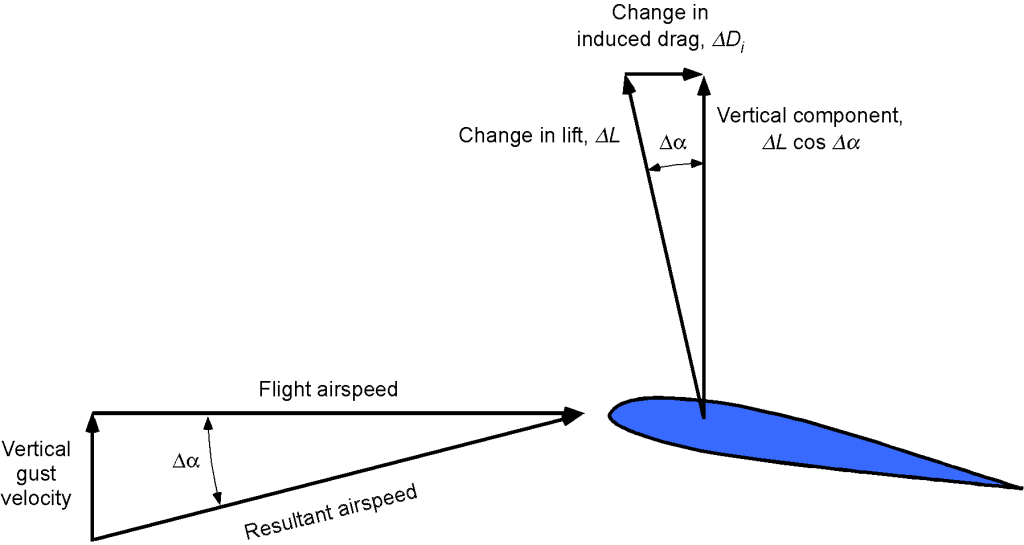
The change in the angle of attack on the wing will be

(27) $\begin{equation*} \Delta \alpha = \tan^{-1} \left( \frac{W_g}{V_{\infty}}\right) \approx \frac{W_g}{V_{\infty}} \mbox{~for small angles} \end{equation*}$

where $W_g$ is denoted here as the vertical gust velocity. If the lift-curve slope of the wing is $C_{L_{\alpha}}$ then the change in lift coefficient will be

(28) $\begin{equation*} \Delta C_L = C_{L_{\alpha}} \left( \frac{W_g}{V_{\infty}} \right) \end{equation*}$

and the change in the lift is

(29) $\begin{equation*} \Delta L = \frac{1}{2} \varrho_{\infty} V_{\infty}^2 S C_{L_{\alpha}} \left( \frac{W_g}{V_{\infty}} \right) = \frac{1}{2} \varrho_{\infty} V_{\infty} S C_{L_{\alpha}} W_g \end{equation*}$

The change in the load factor is then

(30) $\begin{equation*} \Delta n = \frac{\Delta L}{W} = \frac{1}{2} \varrho_{\infty} V_{\infty} \left( \frac{S}{W} \right) C_{L_{\alpha}} W_g \end{equation*}$

Therefore, the total load factor on the airplane compared to straight-and-level unaccelerated flight is

(31) $\begin{equation*} n = 1 + \Delta n = 1 + \frac{1}{2} \varrho_{\infty} V_{\infty} \left( \frac{S}{W} \right) C_{L_{\alpha}} W_g = 1 + \frac{\frac{1}{2} \varrho_{\infty} V_{\infty} C_{L_{\alpha}} W_g}{W/S} \end{equation*}$

There are two interesting observations from Eq. 31:

1. The load factor for a given gust intensity decreases with increasing wing loading, $W/S$ . This outcome means smaller, lighter airplanes (generally with relatively lower wing loadings) tend to respond much more to gusts than larger airplanes such as jet airliners. In this regard, smaller airplanes must be carefully flown at or below the maneuvering airspeed in turbulent air to prevent structural damage.

2. The load factor for a given gust intensity varies linearly with airspeed. So, lines with different values of $W_g$ can be plotted on the $V$ – $n$ diagram, an example being shown in the figure below. These sets of straight lines give the load factor produced on the airplane at a given airspeed from the effects of gusts. When one of these lines intersects the maximum (or minimum) load factor limit, the corresponding airspeed is the maximum airspeed that can be flown without either stalling the wing or exceeding the maximum allowable structural load factor. Each airplane type will have its own specific envelope regarding gust magnitudes and airspeeds.

A representative gust envelope for an airplane in terms of load factor versus airspeed. The magnitude of the gust to which the airplane must be designed depends on its class and type.

The airplane’s resulting load factor may cross over the allowable limit load if the gust is sufficiently severe. However, it cannot exceed the ultimate load without significant structural damage or failure. Even if the limit load factor is exceeded in flight, minor damage may still have occurred (e.g., wrinkled skin panels from buckling), and the airplane must be carefully inspected before further flight.

Corner Airspeed

Notice that if the airplane is flying slower than the corner airspeed (remember this is marked as $V_A$ or $V_a$ on the $V$ – $n$ diagram), any large gust will cause an angle-of-attack to exceed the value for maximum lift coefficient and so cause the airplane to stall. Suppose the airplane is flown at or below its maximum maneuvering speed. In that case, neither an atmospheric gust nor abrupt control movements (such as a rapid pull-up maneuver using full-up elevator) will be sufficient to cause the airplane to exceed its maximum structural load factor. Consequently, when encountering very turbulent air, the airplane should be flown at or below the maximum maneuvering speed so that any gusts and/or control inputs cannot exceed its structural limit loads.

Regulations and the FARs

The FARs define the values of the vertical gust velocities, as shown in the table below. $V_B$ is the design speed for maximum gust intensity, which assumes that the airplane is in straight-and-level flight when it encounters the gust and that the effects of the gust are produced instantaneously. The gust value of “66 ft/s” is based on statistical information gathered about turbulence in the lower atmosphere and is the most extreme case considered representative of all-weather flying. The other values also are based on atmospheric gust statistics. They are used in airplane design to ensure the airplane is strong enough to withstand all anticipated structural loads in turbulent conditions. $V_c$ is the design cruise speed; for airplanes in the transport category (airliners), $V_C$ must not be less than $V_B$ + 43 kts. $V_D$ is based on allowable gusts at the maximum dive speed.

Values of vertical gust velocity specified for airplane design. Between 20,000 ft and 50,000 ft the gust intensity is linearly interpolated.
Airspeed	Below 20,000 ft	Above 50,000 ft
$V_B$ (rough air gust)	66 ft/s	38 ft/s
$V_C$ (gust at max. design speed)	50 ft/s	25 ft/s
$V_D$ (gust at max. dive speed)	25 ft/s	12.5 ft/s

Summary & Closure

It is essential to establish an airplane’s maneuver and gust envelope so that it can be suitably designed to carry all expected flight loads, plus a margin of safety. Airplanes cannot be infinitely strong, so the $V-n$ diagram must be consistent with the airplane’s intended purpose. The final performance capabilities of the airplane will be limited by its aerodynamic capabilities and/or the structural strength of its airframe. Gusts in the atmosphere cause loads on the airplane over and above those produced in smooth air. All airplanes must be designed to be strong enough to carry the normally expected flight loads and the extra loads induced from encounters with turbulent air. The FARs define these gust conditions depending on the type of airplane. It is reassuring that the structural margins built into certified aircraft designs are significant. Even when encountering the most severe turbulence, one can be confident that the aircraft will be strong enough to withstand the anticipated flight loads.

5-Question Self-Assessment Quickquiz

For Further Thought or Discussion

Think about some structural issues in designing a wing for a fully aerobatic airplane. Hint: Include both normal and inverted flight.
What factors other than aerodynamic or structural may limit the acrobatic maneuver limits?
Compare the relative load factors in response to the same vertical gust at the same airspeed that would be produced on the following airplanes: a glider, single-engine general aviation airplane, and a small business jet.

Other Useful Online Resources

To understand more about an airplane’s maneuvering flight envelope and the effects of gusts, then follow up with some of these online resources:

Good video explaining the significance of load factor.
The effects of banking angle on load factor – a DELFT video.
What is load factor and how it relates to a “V-n” diagram – a good video.
A piloting interpretation of the a load factor diagram and critical airspeeds.

License

Icon for the Creative Commons Attribution-NonCommercial-NoDerivatives 4.0 International License

Introduction to Aerospace Flight Vehicles Copyright © 2022–2024 by J. Gordon Leishman is licensed under a Creative Commons Attribution-NonCommercial-NoDerivatives 4.0 International License, except where otherwise noted.

Digital Object Identifier (DOI)

https://doi.org/https://doi.org/10.15394/eaglepub.2022.1066.n39