Rockets & Launch Vehicle Performance

J. Gordon Leishman

47 Rockets & Launch Vehicle Performance

Introduction

Rockets are used to launch payloads, such as satellites and space probes, into Earth orbit. Launch vehicles are highly specialized and tailored to specific missions and payloads. For example, some launch vehicles are designed to place payloads such as satellites into low Earth orbit, while others are intended to send spacecraft into deep space. The choice of the launch vehicle will depend on various factors, including the desired orbit and payload mass and size. In addition to military and civilian applications, there is also a growing interest in commercial and tourism-related payloads. Companies like SpaceX and Blue Origin are developing launch vehicles that can be used for both commercial satellite launches and human spaceflight, which can open space to a broader range of users and applications.

Solid and liquid propellant rocket engines are commonly used for launch vehicles and can be combined to achieve specific performance characteristics. Solid-fuel rocket boosters can provide high initial thrust at liftoff. In contrast, liquid propellant engines can provide more precise control of the thrust generated and greater efficiency once the vehicle is in flight. In addition, the number of stages in a launch vehicle can vary depending on the mission requirements. Some launch vehicles have only one stage, while others have multiple stages that are separated sequentially during flight. The multi-stage approach allows the payload to achieve higher velocities and altitudes than possible with a single-stage rocket design.

Learning Objectives

Appreciate the types of rockets and launch vehicles and their applications to space missions.
Know how to derive and use the rocket equation to solve simple problems such as determining burnout velocities.
Understand the staging process and why it is used for launch vehicles.
Know about missiles and the ballistics of projectiles.

Types of Rockets

There are various types of rockets designed for different purposes and applications. Launch vehicles transport payloads into space. Commercial rockets provide satellite launch services, with some being reusable to reduce costs. Crewed spacecraft launch vehicles, like SpaceX’s Falcon 9, can transport humans to orbit. Space probes explore celestial bodies, suborbital rockets facilitate space tourism, and military rockets and missiles serve defense purposes. Experimental rockets, like research and hobbyist rockets, cater to scientific experiments and personal projects. The diversity in rocket types reflects the multifaceted nature of space exploration, defense, and scientific research.

Launch Vehicles

A representative launch profile of a rocket designed to send a payload into space is shown in the figure below. At the moment of the initial launch, the thrust produced by the engines will be greater than the rocket’s weight, so it accelerates away quickly from the pad. The rocket’s weight rapidly decreases because of the high fuel consumption, so it continues accelerating as it gains altitude. As the rocket begins to exit the atmosphere, which is about 60,000 ft (approximately 20,000 m), it will fly at supersonic velocities. It also begins to pitch to a more horizontal flight path, and the rocket gains translational velocity for the payload to reach its initial equilibrium orbital velocity and altitude.

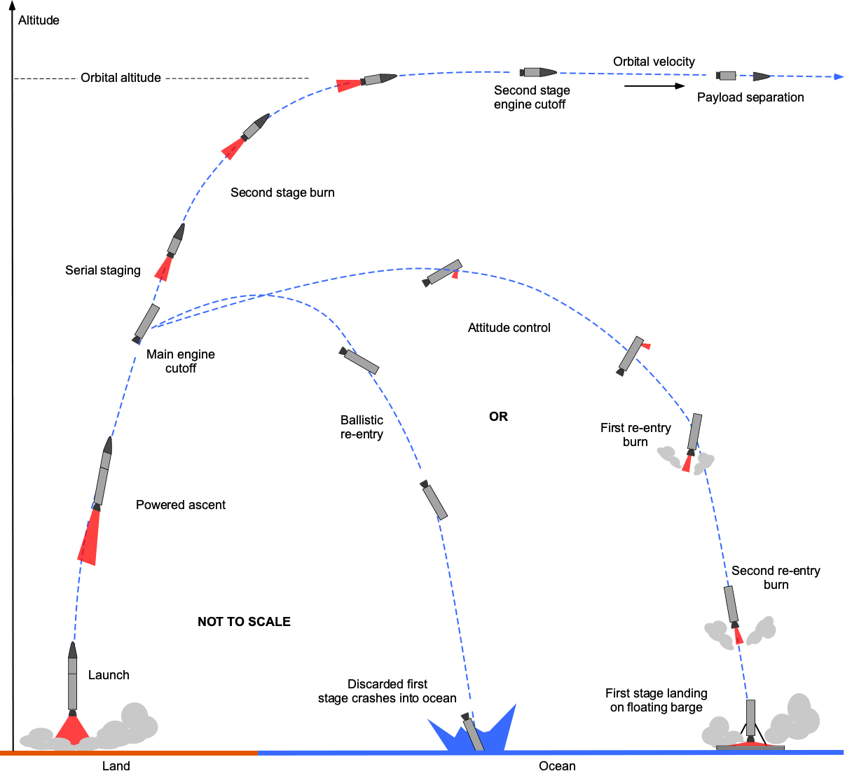
A representative launch profile for a two-stage rocket. The first stage may be recovered by parachute, burn up, or break up and crash into the sea. First-stage recovery significantly reduces the launch costs.

Several minutes into the ascent, staging will occur where the first stage is jettisoned and the rocket engine for the second stage is ignited. The first stage then falls back to the surface and either burns up in the atmosphere (depending on the staging altitude) or breaks apart and crashes into the ocean. In exceptional cases, the first stage may be recovered; solid rocket boosters are usually recovered by parachute and may be reused.

The upper stage (or stages) then continues to accelerate into space. The rocket engines will cut off as the payload reaches the required initial orbital velocity and altitude, which is called a parking orbit. A second burn is then performed after the orbit has stabilized to place the spacecraft into the final orbit, at which point the payload, such as a satellite, will be deployed.

Spacecraft

Spacecraft are used in many different applications. Some are designed for specialist missions, such as planetary exploration or Earth observation, while others have a more general-purpose application and can be used for multiple tasks. Spacecraft typically consist of numerous sub-systems and components, including a payload (the primary equipment or instruments for the mission), a propulsion system (to maneuver and adjust the spacecraft’s trajectory), communication systems (to transmit and receive data), and power systems (such as solar panels or batteries).

One essential function of a spacecraft is orbit insertion, which involves placing the spacecraft into a specific orbit around a planet or other celestial body. This goal requires a carefully planned trajectory and precise firings of the rocket engines to achieve the desired orbit. However, spacecraft can be highly complex and require extensive testing and development on Earth to ensure their reliability and safety in the space environment. This work includes testing in simulated space environments and rigorous quality control procedures to ensure all components meet strict performance standards to minimize the risk of malfunctioning in space, which is inevitably disastrous and a substantial financial loss.

Missiles

Missiles can be broadly divided into ballistic missiles and cruise missiles. Ballistic missiles are used for long-range strikes against threats. They are launched high into the upper atmosphere or the fringes of space, following a parabolic trajectory before reentering the atmosphere and striking their target. Ballistic missiles can be easier to intercept than cruise missiles because they follow a predetermined flight path that is challenging to alter after the launch.

Cruise missiles are designed to fly at low altitudes and follow a more maneuverable flight path to evade threats and defenses. They can be launched from various platforms, including aircraft, ships, and ground-based launchers. They can be more challenging to detect and intercept because they fly at lower altitudes than ballistic missiles and are fast and highly maneuverable.

In addition to their propulsion system, targeting, guidance, and warhead systems, missiles require advanced sensors and communication systems to navigate to their targets and avoid obstacles accurately. Consequently, missiles are highly complex weapons systems that require extensive testing and development to ensure their reliability and effectiveness. In addition, they are subject to strict regulations and controls, and their use is governed by international law.

Miscellaneous

Sounding rockets gather data on atmospheric conditions, such as temperature, pressure, and wind speed, at altitudes that are difficult to reach with aircraft or balloons. They are typically small, single-stage rockets launched into suborbital trajectories that carry scientific instruments and sensors to collect various types of data.

Jet-Assisted Takeoff (JATO), also known as Rocket-Assisted Takeoff (RATO), is a technique that uses rockets to provide additional thrust during an aircraft’s takeoff, particularly when the aircraft is heavily loaded or taking off from a short runway. The rocket engines temporarily boost the aircraft’s acceleration, helping it take off and climb. The most famous RATO aircraft is a modified Lockheed Martin C-130 Hercules, a four-engine turboprop military transport aircraft that serves as a utility aircraft for the Blue Angels. The RATO system includes solid rocket engines attached to the sides of the aircraft’s fuselage.

Rockets are also used to provide emergency lifelines to ships that are in distress. In this application, a rocket-powered line is fired from shore or another ship to the stranded vessel, enabling rescuers to establish a connection and provide assistance. Rockets could also deliver relief materials to inaccessible areas during natural disasters or humanitarian crises. However, this approach would require developing reliable and cost-effective rocket delivery systems, appropriate infrastructure, and logistical support.

Rocket Equation

The rocket equation finds considerable use in rocket sizing and propellant load estimations. The derivation of this equation is credited to the Russian scientist Konstantin Tsiolkovsky, who published it in 1903. However, Robert Goddard and Hermann Oberth also derived the rocket equation, independently of Tsiolkovsky (and each other), during the 1920s.

Derivation

Consider an accelerating rocket of mass $M$ , where the engine’s thrust is used to propel it, as shown in the figure below. Using Newton’s second law, then

(1) $\begin{equation*} T = M \left( \frac{dV}{dt} \right) \end{equation*}$

where $dV/dt$ is the acceleration of the rocket. The forces from gravity and atmospheric drag have been neglected relative to the rocket’s weight, so the equation is strictly valid for a rocket in space. However, it is not an unreasonable approximation otherwise, including flight in the atmosphere.

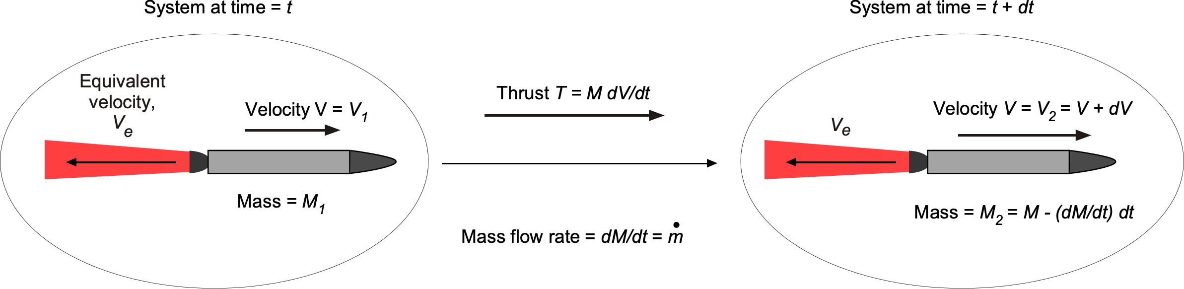
The derivation of the rocket equation uses the basic principles of momentum conservation.

The thrust produced by the rocket motor is

(2) $\begin{equation*} T = \overbigdot{m} V_{\rm eq} \end{equation*}$

where $\overbigdot{m}$ is the mass flow rate of propellant during the burn, and $V_{\rm eq}$ is the equivalent exhaust velocity from the nozzle of the rocket motor. Using Eq. 1, then

(3) $\begin{equation*} M \left( \frac{dV}{dt} \right) = \overbigdot{m} V_{\rm eq} \end{equation*}$

which gives the acceleration of the rocket during the burn as

(4) $\begin{equation*} \frac{dV}{dt} = \left( \frac{\overbigdot{m}}{M} \right) V_{\rm eq} \end{equation*}$

The change in mass of the rocket is $-dM$ (from the use of propellant), so the time rate of decrease of mass is equal to the mass flow rate, i.e.,

(5) $\begin{equation*} -\frac{dM}{dt} = \overbigdot{m} \end{equation*}$

so that

(6) $\begin{equation*} dV = -\left( \frac{dM}{M} \right) V_{\rm eq} \end{equation*}$

Separating the variables and integrating over the burn time gives

(7) $\begin{equation*} \int_{V_1}^{V_2} dV = -V_{\rm eq} \int_{M_0}^{M_b} \left( \frac{dM}{M} \right) \end{equation*}$

where $M_1$ and $V_1$ are the initial mass and velocity of the rocket at $t = t_1$ , respectively, and $M_2$ and $V_2$ are the final mass and velocity, respectively, at time, $t_2$ . After integration of the previous equation, the change in the velocity of the rocket is

(8) $\begin{equation*} V_2 - V_1 = \Delta V = V_{\rm eq} \ln \left( \frac{M_1}{M_2} \right) \end{equation*}$

This latter equation, which is called the rocket equation, is very useful in mission performance analysis and vehicle sizing. In some ways, it is analogous to the Breguet equations used for aircraft performance. Notice that $M_2$ is given by

(9) $\begin{equation*} M_2 = \overbigdot{m} \left( t_2 - t_1 \right) = M_1 - M_p \end{equation*}$

where $M_p$ is the mass of propellant used.

The rocket equation is often written in terms of the initial mass, $M_0$ , and the burnout mass, $M_b$ , i.e., the mass of the rocket after the propellant is fully expended, as

(10) $\begin{equation*} V_b - V_0 = \Delta V = V_{\rm eq} \ln \left( \frac{M_0}{M_b} \right) \end{equation*}$

where $V_0$ is the initial velocity, and the burnout velocity is $V_b$ . Notice that for a launch vehicle, its initial velocity on the pad is zero ( $V_0 = 0$ ), so the burnout velocity for the rocket (or the first stage) will be is

(11) $\begin{equation*} V_b = V_{\rm eq} \ln \left( \frac{M_0}{M_b} \right) = V_{\rm eq} \ln \left( \frac{M_0}{M_0 - M_p} \right) \end{equation*}$

Effects of Gravity

If gravity is included (but no aerodynamic drag) in the case of a pure vertical launch, then the rocket equation in Eq 10 is modified to

(12) $\begin{equation*} \Delta V = V_{\rm eq} \ln \left( \frac{M_0}{M_b} \right) - \Delta V_g \end{equation*}$

The second term, $\Delta V_g$ , is called the gravity loss. Notice that for a rocket going up vertically, then the gravity loss term reduces the attainable velocity at the burnout time, i.e.,

(13) $\begin{equation*} \int_0^{t_b} g_0 \, dt = g_0 \, t_b = \Delta V_g \end{equation*}$

where $g_0$ is standard gravity; $g_0$ is equal to 9.81 m/s $^2$ or 32.17 ft/s $^2$ . Therefore, the rocket equation with the gravity loss term becomes

(14) $\begin{equation*} \Delta V = V_{\rm eq} \ln \left( \frac{M_0}{M_b} \right) - g_0 \, t_b = V_{\rm eq} \ln \left( \frac{M_0}{M_0 - M_p} \right) - g_0 \, t_b \end{equation*}$

If the rocket follows a curved trajectory and pitches over at a local trajectory angle $\gamma$ (with respect to the horizon) as it increases altitude, then

(15) $\begin{equation*} \Delta V_g = \int_0^{t_b} \sin \gamma \, g_0 \, dt \end{equation*}$

where $\gamma = 90^{\circ}$ when the rocket flies vertically and $\gamma = 0$ when it flies horizontally. However, properly evaluating this latter term requires more specific information about the launch profile. It is usually sufficient to neglect the gravity loss term as its value is relatively small.

Burnout Height

The vertical height achieved at the burnout time, $t_b$ , is

(16) $\begin{equation*} H_b = \int_0^{t_b} V \, dt \end{equation*}$

If the flight velocity, $V$ , is given by

(17) $\begin{equation*} V = V_{\rm eq} \ln \left( \frac{M_0}{M_b} \right) - g_0 \, t_b \end{equation*}$

then the height achieved at $t_b$ can be shown to be

(18) $\begin{equation*} H_b = V_{\rm eq} t_b \left( \frac{ \ln \left( \displaystyle{\frac{M_0}{M_b}} \right) }{\displaystyle{\frac{M_0}{M_b} - 1} } \right) - \frac{1}{2} g_0 \, t_b^2 \end{equation*}$

Rocket Mass Breakdown

The initial mass $M_0$ of the rocket vehicle can be written as the sum

(19) $\begin{equation*} M_0 = M_P + M_S + M_L \end{equation*}$

where $M_P$ is the mass of the propellant, $M_S$ is the structural mass, and $M_L$ is the mass of the payload. The burnout mass is reached when all of the propellant is exhausted, which is given by

(20) $\begin{equation*} M_b = M_0 - M_P = M_S + M_L \end{equation*}$

Therefore, the initial mass-to-burnout mass ratio, $R$ , is defined as

(21) $\begin{equation*} R = \frac{M_0}{M_b} \end{equation*}$

The payload ratio, $\lambda$ , is defined by

(22) $\begin{equation*} \lambda = \frac{M_L}{M_0 - M_L} = \frac{M_L}{M_P + M_S} \end{equation*}$

Finally, the structural mass coefficient, $\epsilon$ , is defined by

(23) $\begin{equation*} \epsilon = \frac{M_S}{M_P + M_S} = \frac{M_S}{M_0 - M_L} \end{equation*}$

In light of these preceding definitions, it can be shown that the mass ratio $R$ is given by

(24) $\begin{equation*} R = \frac{M_0}{M_b} = \frac{1 + \lambda}{\epsilon + \lambda} \end{equation*}$

Therefore, in terms of the mass and payload ratios and the structural mass coefficient, then

(25) $\begin{equation*} \Delta V = V_{\rm eq} \ln R = V_{\rm eq} \ln \left( \frac{1 + \lambda}{\epsilon + \lambda} \right) \end{equation*}$

Payload mass ratios can vary considerably from mission to mission. However, structural mass coefficients are found to be relatively constant based on historical data for various types of rockets and launch vehicles. Also, the value of the structural mass coefficient, $\epsilon$ , is relatively similar for different vehicles based on historical data, which is convenient for preliminary design purposes when this value needs to be estimated.

Impulse

The total impulse is defined as the integral of the thrust over its burnout time, $t_b$ , i.e., the time for which the rocket engine runs. The total impulse is given by

(26) $\begin{equation*} I = \int_0^{t_b} T \, dt = \int_0^{t_b} \overbigdot{m} V_{\rm eq} \, dt \end{equation*}$

as illustrated graphically in the figure below.Notice that the impulse is simply the area under the thrust/time curve.

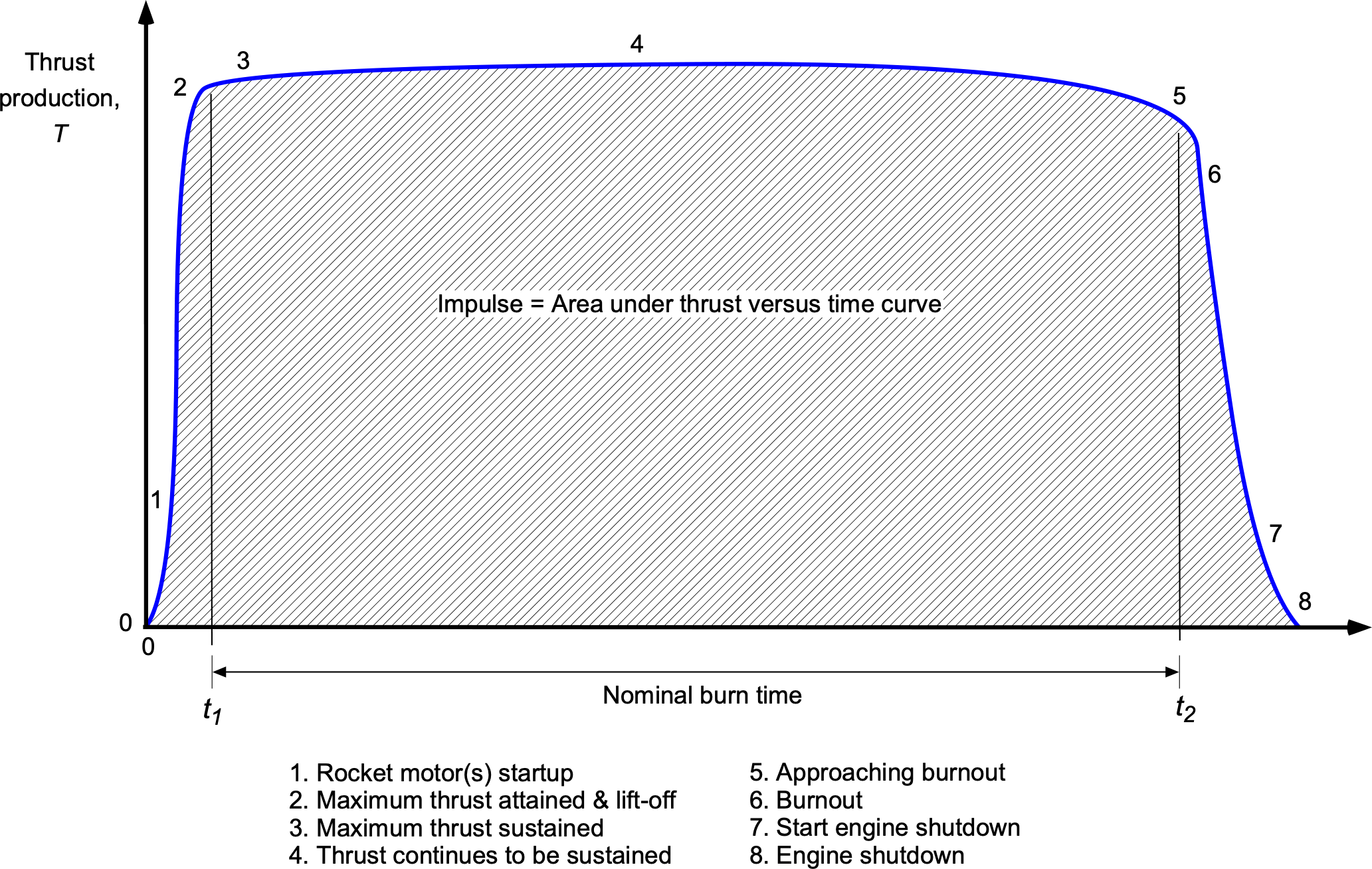
The impulse is defined as the integral of the thrust over the burnout time, which is equal to the net momentum imparted to the rocket.

If $\overbigdot{m}$ and $V_{\rm eq}$ are constant, as is often a good approximation, then

(27) $\begin{equation*} I = T\, t_b = M_P \, V_{\rm eq} \end{equation*}$

where $M_P$ is the mass of the propellant burned. The total impulse, therefore, will be equivalent to the net momentum imparted to a rocket by the engine during the burn.

Specific Impulse

The measure of efficiency used in most rocket performance calculations is the specific impulse, which is the thrust divided by the propellant flow rate. In general, one wishes to carry as little propellant as possible. The specific impulse, $I_{\rm sp}$ , is

(28) $\begin{equation*} I_{\rm sp} = \frac{\mbox{\small Total~impulse}}{\mbox{\small Weight~of~propellant~burned}} = \frac{I}{M_P \, g_0} \end{equation*}$

Therefore, the higher the value of $I_{\rm sp}$ the more efficient the rocket motor will be in producing thrust.

It is further apparent using Eq. 2 that

(29) $\begin{equation*} I_{\rm sp} = \frac{V_{\rm eq}}{g_0} = \frac{T}{\overbigdot{m} \, g_0} \end{equation*}$

where it will be noticed that $I_{\rm sp}$ has units of time (seconds). Therefore, the specific impulse is the total impulse (or change in momentum delivered) per unit weight of the propellant consumed, which is a measure of the efficiency in producing thrust. Therefore, the higher the value of the specific impulse then, the more efficient the rocket motor is in producing thrust.

Worked Example #1 – Burnout velocity of a single-stage rocket

Use the rocket equation to determine the burnout velocity and the maximum achievable height of a simple rocket, assuming that it is launched vertically. Neglect the aerodynamic drag forces. Solve for the burnout velocity and maximum altitude if the burnout time is 60 seconds. The specific impulse is 250 seconds, the initial mass is 12,700 kg, and the propellant mass is 8,610 kg.

Show solution/hide solution

The rocket equation gives the change in the velocity of the vehicle $\Delta V$ , i.e.,

$\Delta V = V_{\rm eq} \ln \left( \frac{M_0}{M_b} \right)$

where $M_0$ is the initial mass of the vehicle and $M_b$ is the final or burnout mass. If gravity is included (but no aerodynamic drag), then

$\Delta V = V_{\rm eq} \ln \left( \frac{M_0}{M_b} \right) - g_0 \, t_b.$

where $t_b$ is the burnout time, which is 60 seconds in this case.

The equivalent velocity $V_{\rm eq}$ is given in terms of the specific impulse, i.e.,

$V_{\rm eq} = I_{\rm sp} \, g_0 = 250 \times 9.81 = 2,452.5~\mbox{m/s}$

and the burnout mass $M_b$ is given by

$M_b = M_0 - M_P = 12,700 - 8,610 = 4,090~\mbox{kg}$

The burnout velocity is given by the rocket equation, i.e.,

$\Delta V = V_{\rm eq} \ln \left( \frac{M_0}{M_b} \right) - g_0 \, t_b$

Therefore, $\Delta V$ at the burnout is

$\Delta V = 2,778.16 - 9.81 \times 60 = 2,778.16 - 588.6 = 2,189.56~\mbox{m/s}$

which is 2.19 km/s. Assuming the rate of fuel consumption is constant, then the mass of the rocket $M$ varies over time as

$M = M_0 - M_P \left( \frac{t}{t_b} \right) = M_0 - \left( M_0 - M_b \right) \left( \frac{t}{t_b} \right)$

The velocity of the rocket is

$V = V_{\rm eq} \ln \left( \frac{M_0}{M} \right) - g_0 \, t$

The height achieved at the burnout time, $t_b$ , is

$H_b = V_{\rm eq} t_b \left( \frac{ \ln \left( \displaystyle{\frac{M_0}{M_b}} \right) }{\displaystyle{\frac{M_0}{M_b} - 1} } \right) - \frac{1}{2} g_0 \, t_b^2$

Inserting the values gives

$H_b = 2,452.5 \times 60 \left( \frac{ \ln \left( \displaystyle{\frac{12,700}{4,090}} \right) }{\displaystyle{\frac{12,700}{4,090} - 1} } \right) - \frac{1}{2} \times 9.81 \times 60^2$

Therefore, the height achieved is

$H_b = 2,452.5 \times 60 \left( \frac{1.133}{2.105} \right) - \frac{1}{2} \times 9.81 \times 60^2 = 61.54~\mbox{km}$

The rocket’s final additional coasting height can then be determined by equating its kinetic energy at its burnout time with its change in potential energy between that point and the maximum obtained height.

Launching into Orbit

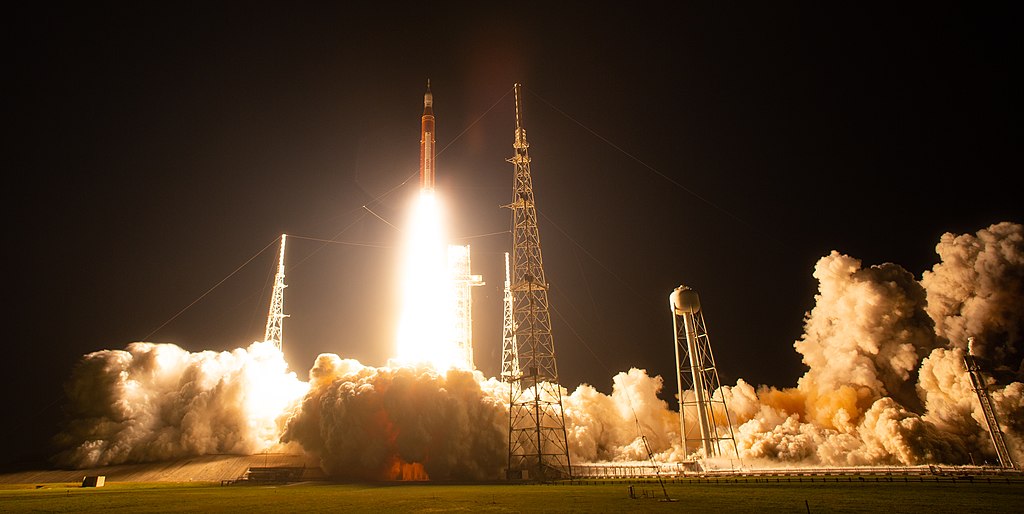
Rocket launches are hugely exciting events to watch! The synchronized launch process, the flaming exhaust, and clouds of smoke, followed by the rising spacecraft into the sky, can be awe-inspiring. The technology and engineering behind the launches, the science and exploration they enable, and the thrill of human endeavor all contribute to the excitement. Additionally, watching a rocket launch live or on YouTube can be an educational and inspiring experience, especially for students and younger people interested in science and space. Even those who live in Florida are never tired of watching rocket launches!

NASA’s SLS rocket carrying the Orion spacecraft launches on the Artemis 1 flight on November 16, 2022, from Launch Complex 39B at NASA’s Kennedy Space Center in Florida.

Using the Rocket Equation

Drama and excitement aside, the energy and propellant requirements for a rocket (booster) and its payload with the $\Delta V$ needed to reach a specific orbital altitude $h_s$ can be estimated using the principles of energy conservation in conjunction with Tsiolkovsky’s rocket equation. The rocket equation is given as

(30) $\begin{equation*} \Delta V = V_{\rm eq} \ln \left( \frac{M_0}{M_b} \right) \end{equation*}$

where $V_{\rm eq}$ is the equivalent exit velocity from the particular rocket engine, $M_0$ is the initial mass of the rocket or spacecraft at the beginning of the burn, and $M_b$ is the final (burnout) mass after the burn at burnout time, $t_b$ , during which a propellant mass $M_P$ is consumed. In this case, it is assumed, for simplicity, that it is a single-stage vehicle (i.e., no staging).

The equivalent exit velocity can be written in terms of the specific impulse, $I_{\rm sp}$ , as

(31) $\begin{equation*} V_{\rm ex} = I_{\rm sp} \, g_0 \end{equation*}$

where $g_0$ is the reference value of acceleration under gravity at mean sea-level on Earth, i.e., $g_0 = 9.81$ m/s. Therefore, the rocket equation can also be written as

(32) $\begin{equation*} \Delta V = I_{\rm sp} \, g_0 \ln \left( \frac{M_0}{M_b} \right) \end{equation*}$

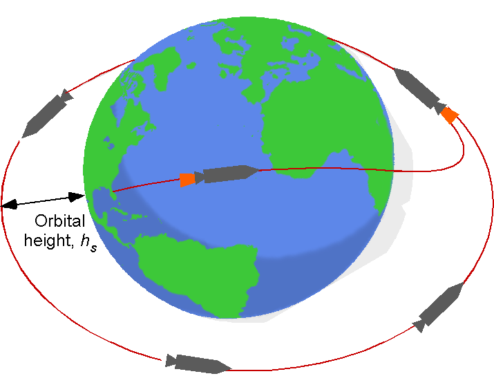
where the value of $I_{\rm sp}$ depends on the type of rocket engine and its propellant. If the value of $I_{\rm sp}$ is known, then the rocket equation can be used to determine the propellent mass needed to give a certain $\Delta V$ for the satellite or spacecraft to reach an orbit at the required altitude, $h_s$ , as shown in the figure below.

Illustrating of rocket reaching orbital height around Earth. — Orbital mechanics can be used to estimate the propellent mass needed to lift a payload into orbit.

For a launch, several factors can influence the $\Delta V$ required, i.e.,

The needed orbital altitude above the surface of the Earth, $h_s$ .
The orbital inclination relative to the Earth’s equatorial plane.
The launch latitude from the Earth (this affects the initial energy).
The effects of overcoming gravity (when the rocket goes vertically).
The aerodynamic drag on the rocket in the lower atmosphere.

Kinetic Energy

For the satellite or spacecraft to reach the required orbital altitude, $h_s$ , then the $\Delta V$ required for the needed kinetic energy is

(33) $\begin{equation*} \Delta V = \sqrt{ \frac{G \, M_E}{R_E + h_s} } \equiv \Delta V_K \end{equation*}$

noting that this result does not depend on the mass of the satellite or spacecraft. This latter component is the dominant energy requirement for high orbits.

Potential Energy

The $\Delta V$ associated with creating the needed potential energy for the same orbit is

(34) $\begin{equation*} \Delta V = \sqrt{ \frac{ G \, M_E }{R_E} } \sqrt{ 2 - \frac{R_E}{R_E + h_s} } - \sqrt{ \frac{ G \, M_E}{R_E + h_s} } \equiv \Delta V_U \end{equation*}$

For low orbital altitudes with $h \ll R_E$ , then

(35) $\begin{equation*} \Delta V_U = \frac{h_s}{R_E} \sqrt{ \frac{G \, M_E}{R_E} } \end{equation*}$

which is the dominant term in this case compared to the kinetic energy.

Gravity Effect

A gravitational effect must be added to the total needed $\Delta V$ , usually called gravity loss. For a rocket going up vertically, then

(36) $\begin{equation*} \Delta V_g = \int_0^{t_b} g_0 \, dt = g_0 \, t_b \end{equation*}$

where $t_b$ is the burnout time. If the rocket follows a curved trajectory and pitches over at a local trajectory angle $\gamma$ (with respect to the horizon) as it increases altitude, then

(37) $\begin{equation*} \Delta V_g = \int_0^{t_b} \sin \gamma \, g_0 \, dt \end{equation*}$

where $\gamma = 90^{\circ}$ when the rocket flies vertically and $\gamma = 0$ when it flies horizontally. Therefore, properly evaluating this latter term requires information about the launch profile.

Aerodynamic Effects

There is an aerodynamic drag on the rocket as it flies through the lower atmosphere, contributing to the needed propellant requirements. This drag force, $D$ , can be expressed as

(38) $\begin{equation*} D = \frac{1}{2} \varrho V_{\infty}^2 \, C_D \, A_{\rm ref} = q \, C_D \, A_{\rm ref} \end{equation*}$

where $q$ is the dynamic pressure, i.e., $q = \frac{1}{2} \varrho V_{\infty}^2$ where $\varrho$ is the local density of the air, and $V_{\infty}$ is the true airspeed, the latter values also requiring information about the launch profile. The density of the air can be represented by an ISA model for both the low and extended atmospheres. The reference area, $A_{\rm ref}$ , in Eq. 38 is usually taken as the projected frontal area of the rocket. The drag coefficient, $C_D$ , will also depend on the overall shape of the rocket and its flight Mach number.

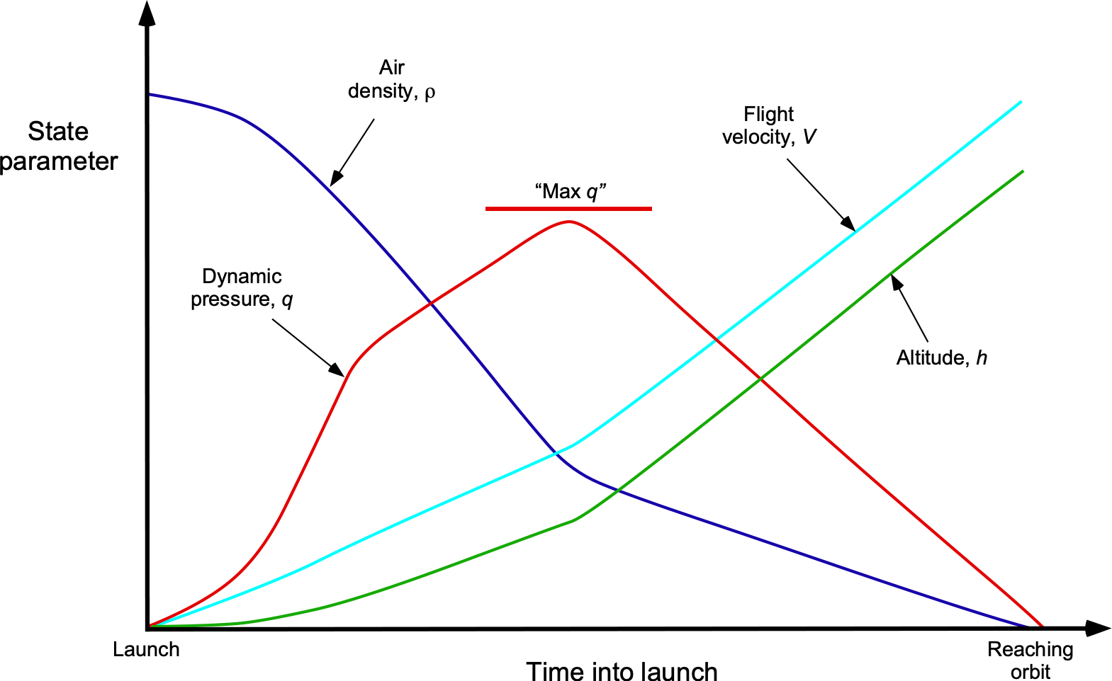
The rocket’s drag given by Eq. 38 is proportional to the air’s density and the airspeed’s square. This result shows that to minimize the net aerodynamic effects, the rocket should ascend vertically and as slowly as possible, but this is contrary to the need to accelerate the rocket as quickly as possible to minimize gravitational effects. Nevertheless, the dynamic pressure during the launch needs particular emphasis because this quantity affects the aerodynamic-induced structural loads on the rocket.

As shown in the representative launch profile below, the value of $q$ increases rapidly after launch, reaching a maximum and decreasing quickly as the altitude increases and the density of the air diminishes. In many cases, the “maximum $q$ ” value on the rocket will be limited, requiring the rocket engines to be throttled down temporarily to prevent excessive aerodynamic loads on the vehicle.

A representative launch profile for a rocket. The criticality of the “max q” in the flight profile requires that the rocket engines be throttled.

Published aerodynamic drag coefficients for launch vehicles are not generally available. However, some research has been published, including Ballistic Research Laboratories, Memorandum Report No. 545, and NASA TM X-53770. The latter report shows the drag coefficients of the NASA Saturn V launch vehicle as measured in several wind tunnels over a wide range of Mach numbers, a sample of which is shown in the figure below. The reference length used in the results is the diameter of the primary launch vehicle, where $D_{\rm ref}$ = 10.06 meters or 33 feet. The total drag (axial) force is split into forebody drag and base drag. Notice the rapid increase in drag coefficient during the transonic region near Mach = 1, followed by a progressive reduction in drag coefficient in the supersonic regime.

NASA measurements of the aerodynamic drag coefficient on the Saturn V launch vehicle. Notice that the drag is decomposed into forebody and base drag components.

In the absence of any other information, the drag coefficient, $C_D$ , for a rocket is often represented as

(39) $\begin{equation*} C_D =\left \{\begin{array}{ll} 0.2 \quad \mbox{ for $0 < M_{\infty} \leq 0.85$} \\[12pt] 0.11 + \displaystyle{\frac{0.82}{M_{\infty}^2}} - \displaystyle{\frac{0.55}{M_{\infty}^4}} \quad \mbox{for $M_{\infty} > 0.85$} \end{array} \right. \end{equation*}$

where $M_{\infty}$ is the Mach number of the free-stream aerodynamic flow. The $\Delta V$ increment required to overcome aerodynamic drag (again, using the rocket equation) will be

(40) $\begin{equation*} \Delta V_d = \sqrt{ \int_0^{t_a} \frac{D \, V_{\infty}}{M_i} \, dt } \end{equation*}$

where $M_i$ is the instantaneous mass of the rocket and $t_a$ is the launch time over which aerodynamic forces are considered. However, for most launch vehicles, the $\Delta V_d$ velocity losses from aerodynamic drag are small and are typically between 0.05 and 0.15 km/s.

Launch Latitude

The needed $\Delta V$ also depends on the latitude of the launch. The initial energy given to the rocket from the Earth’s rotation is higher for launch sites closer to the equator. The needed $\Delta V$ is lower if the rocket is launched in the direction of the Earth’s rotation (toward the east). For launches from Cape Canaveral, for example, the $\Delta V_{\rm lat}$ boost (i.e., a negative $\Delta V$ ) is about 0.3 km/s and is certainly not insignificant regarding propellant requirements.

Total Delta-V

Therefore, the total needed $\Delta V_T$ is the sum

(41) $\begin{equation*} \Delta V_T = \Delta V_K + \Delta V_U + \Delta V_g +\Delta V_d - \Delta V_{\rm lat} \end{equation*}$

The required propellant mass, $M_P$ , can then be estimated from the rocket equation, i.e.,

(42) $\begin{equation*} \Delta V_T = I_{\rm sp} \, g_0 \ln \left( \frac{M_0}{M_b} \right) = I_{\rm sp} \, g_0 \ln \left( \frac{M_0}{M_0 - M_P} \right) \end{equation*}$

again, assuming no staging. Therefore, using the principles of logarithms, then

(43) $\begin{equation*} \frac{M_0}{M_P} = 1 - \exp \left( -\frac{\Delta V_T}{I_{\rm sp} \, g_0} \right) \end{equation*}$

If staging is used, the $\Delta V$ for each stage would be calculated as each stage is depleted of propellant, and the empty stage is discarded.

Estimating the Escape Velocity from Earth

The mass of the Earth, $M_E$ , is 5.97 $\times 10^{24}$ kg. The radius of an initial orbit will be the radius of the Earth $R_E$ , which is 6.3781 $\times 10^6$ m, plus the orbital height, $h$ . Also, we know that the universal gravitational constant $G$ = 6.67428 $\times 10^{-11}$ N m $^2$ kg $^{-2}$ . Assuming that the orbital height relative to the radius of the Earth is small, then it can be shown that the minimum escape velocity is given by

$V_{\rm esc} = \sqrt{ \frac{2 \, G \, M_E }{R_E} } = \sqrt{ \frac{2 \times (6.67428 \times 10^{-11}) \times (5.97 \times 10^{24}) }{6.3781 \times 10^6 }} = 11.18~\mbox{km/s}$

All spacecraft designed to head out into space away from the Earth must be given a velocity larger than 11.2 km/s, which is fast!

Steering a Rocket

A rocket must be steered along a prescribed flight path so the payload can reach the necessary altitude. A modern rocket (e.g., a launch vehicle) is usually steered along its flight path by gimbaling (rotating) the engine(s) to change the direction of the thrust vector. However, as the figure below summarizes, other means may also be used.

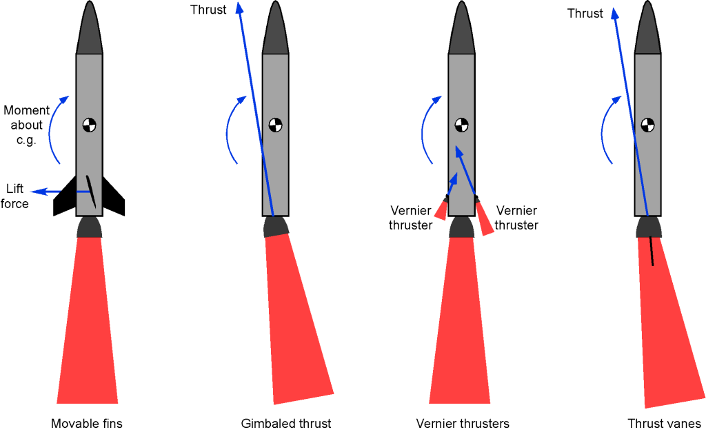
Several methods can be used to steer a rocket. The most common is the gimballed thrust design.

Early rockets used movable aerodynamic surfaces or fins at the rear of the rocket, and this technique is also used on most air-to-air missiles. These surfaces create varying aerodynamic forces and moments on the rocket, which can be used to control its trajectory. Some rockets have used additional vernier rocket engines to give attitude control. However, vernier steered rockets are not used as much because of this system’s extra weight and the different fuel needed. On some early rockets and ballistic missiles, small thrust vanes were placed directly in the exhaust stream of the rocket’s exhaust to produce forces that could be used for steering.

Staged Rocket Vehicles

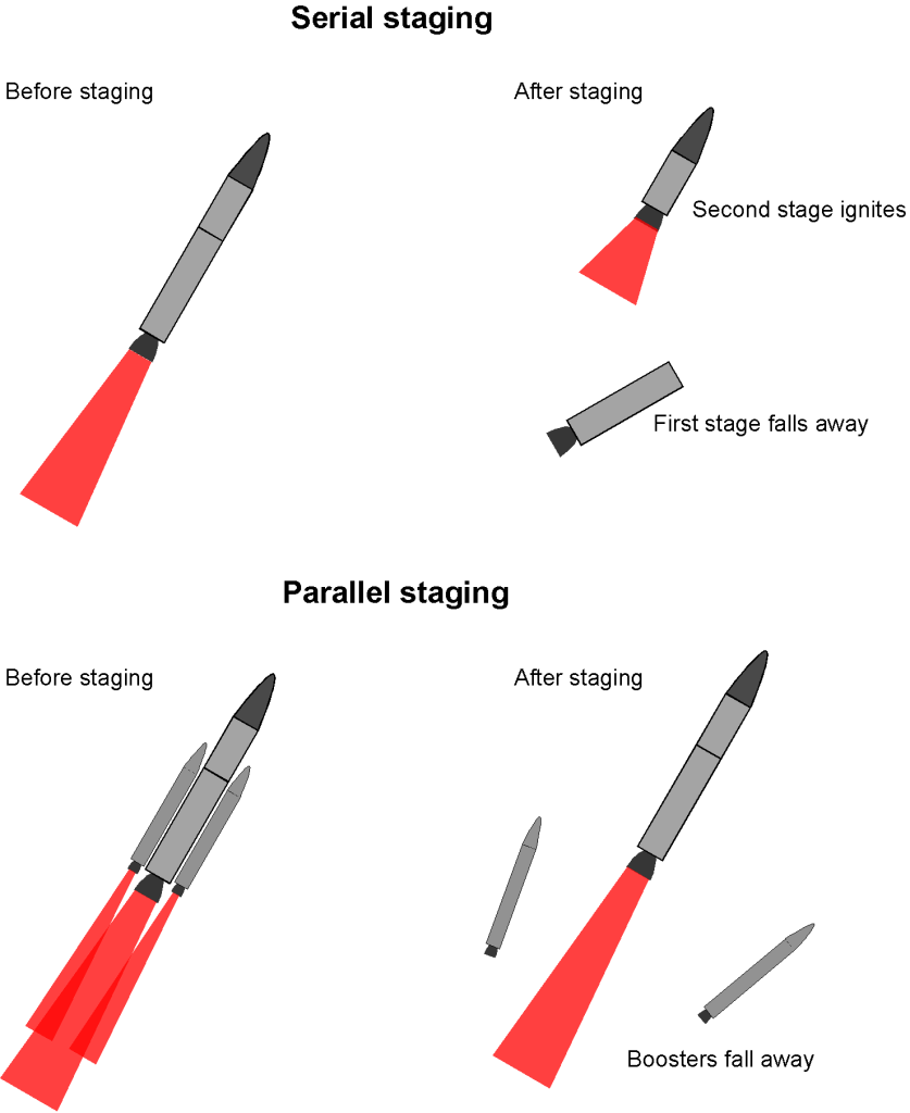
Staging a launch vehicle aims to maximize the payload ratio that can be launched into space. The goal is to launch the largest payload to the required burnout velocity using the least non-payload mass (defined as the structural weight of the rocket plus the fuel). As shown in the figure below, there are two types of staging:

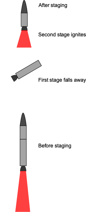
Serial staging, where the stages are ignited, used, and jettisoned in serial sequence.
Parallel staging, where all stages are ignited and used, but the stages are jettisoned as they burn out, e.g., solid rocket boosters.

Staging is essential for maximizing a payload’s orbital velocity and height.

To reach an optimal staging of the launch vehicle, there are four primary considerations:

The initial stages should have the lowest values of $I_{\rm sp}$ , and later stages should have the highest $I_{\rm sp}$ .
The stages with the lower $I_{\rm sp}$ should contribute more to $\Delta V$ .
Each successive stage should be smaller than the previous stage.
Similar stages should provide similar increments to $\Delta V$ .

Serial Staged Rocket

For a serial staged launch vehicle, then

(44) $\begin{equation*} R_i = \frac{M_{0_{i}}}{M_{b_{i}}} ; \quad \lambda_i = \frac{M_{L_{i}}}{M_{0_{i}} - M_{L_{i}}} ; \quad \epsilon_i = \frac{M_{0_{i}}}{M_{P_{i}} + M_{S_{i}}} \end{equation*}$

where the index $i$ refers to the stage number. Also

(45) $\begin{equation*} R_i = \frac{1 + \lambda_i}{\epsilon_i + \lambda_i} \end{equation*}$

For a staged vehicle overall, the $\Delta V$ values are added for each stage, i.e.,

(46) $\begin{equation*} \Delta V = \sum_{i=1}^{N} \Delta V_i = \sum_{i=1}^{N} V_{{\rm eq}_{i}} \ln R_i \end{equation*}$

The structural mass coefficients for a staged launch vehicle are usually similar to those of a single stage. However, payload ratios are generally higher for a staged vehicle. In some cases, finding the maximum allowable structural mass to meet a particular set of payload requirements may be desirable, setting some structural design goals and constraints.

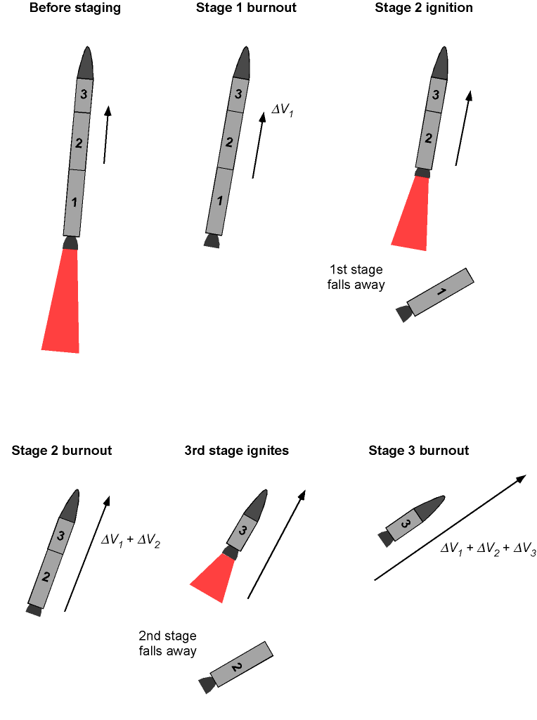
Sequence of staging for a three-stage launch vehicle.

Below is a step-by-step breakdown of the general procedure for calculating the total burnout velocity or time for a multi-stage rocket with serial staging:

1. Divide the rocket as a system into its stages. Each stage is typically characterized by a specific propulsion system or engine and will have its own parameters, such as mass, specific impulse, thrust, and fuel weight or burn time.
2. For each stage, calculate the initial mass, which is the total mass of the rocket at the beginning of the stage burn, and the final mass, which is the rocket’s mass at the end of the stage burn after the propellant has been burned.
3. Calculate the burnout velocity for each stage using the rocket equation. The gravitational force (weight) acting on the rocket must also be considered.
4. Add each stage’s burnout velocity to the previous stage’s initial velocity. Assuming that each stage occurs immediately after the previous one, the burnout velocity of one stage becomes the initial velocity for the next stage.
5. Repeat steps 2–4 for the final stage of the rocket system until the burnout time and/or burnout velocity have been calculated for the final stage carrying the payload mass.

Worked Example #2 – Two-stage rocket calculation

Consider a two-stage rocket with the following design characteristics. Payload mass = 60 kg. First stage: propellant mass = 7,200 kg, structural mass = 800 kg, and the mass flow rate is $\overbigdot{m}$ = 80.0 kg s $^{-1}$ . Second stage: propellant mass = 5,400 kg, structural mass = 600 kg, and the burn time is 100 s. The specific impulse, $I_{\rm sp}$ , for the first and second stages is 275 s. Calculate the following:

For the first stage:

The equivalent exhaust velocity.
The thrust produced.
The total burn time.
The burnout velocity.

For the second stage:

The equivalent exhaust velocity.
The mass flow rate.
The thrust produced.
The final burnout velocity.

Show solution/hide solution

For the first stage:

1. The equivalent exhaust velocity, $V_{{\rm eq}_{1}}$ , is

$V_{{\rm eq}_{1}} = I_{\rm sp_{1}} \, g_0 = 275 \times 9.81 = 2,697.75~\mbox{m/s}$

2. The thrust, $T_1$ , produced is

$T_1 = \overbigdot{m}_1 \, V_{{\rm eq}_{1}} = 80.0\times 2,697.75 = 215,820~\mbox{N}$

3. The total burn time, $t_{b_{1}}$ , is

$t_{b_{1}} = \frac{M_{P_{1}}}{\overbigdot{m}_1}= \frac{7,200}{80.0} = 90.0~\mbox{s}$

4. The initial mass, $M_{0_{1}}$ , is

$M_{0_{1}} = M_{P_{1}} +M_{P_{2}} + M_{S_{1}} + M_{S_{2}} + M_{L}$

and inserting the values gives

$M_{0_{1}} = 7,200 +5,400 + 800 +600 +60 = 14,060~\mbox{kg}$

The burnout mass, $M_{b_{1}}$ , is

$M_{b_{1}} = M_{0_{1}} - M_{P_{1}} = M_{P_{2}} + M_{S_{1}} + M_{S_{2}} + M_{L}$

and with the given values leads to the burnout mass of the first stage as

$M_{b_{1}} = 5,400 + 800 + 600 + 60 = 6,860~\mbox{kg}$

The $\Delta V$ increment for the first stage is

$\Delta V_1 = V_{b_{1}} - 0 = V_{{\rm eq}_{1}} \ln \left( \frac{M_{0_{1}}}{M_{b_{1}}} \right) - g_0 \, t_{b_{1}}$

and inserting the values gives

$V_{b_{1}} = 2,697.75 \ln \left( \frac{14,060}{6,860} \right) - 9.81\times 90 = 1,053.0~\mbox{m/s}$

Therefore, for the first stage, the burnout velocity is

$V_{b_{1}} = 1,053.0~\mbox{m/s}$

Foe the second stage:

1. Because the $I_{\rm sp}$ remains the same for stage 2, the equivalent exhaust velocity will also be the same, i.e.,

$V_{{\rm eq}_{2}} = I_{\rm sp_{2}} \, g_0 = 275 \times 9.81 = 2,697.75~\mbox{m/s}$

2. The mass flow rate, $\overbigdot{m}_2$ , is

$\overbigdot{m}_2 = \frac{M_{P_{2}}}{t_{b_{2}}} = \frac{5,400}{100} = 54.0~\mbox{kg/s}$

3. The thrust $T_2$ produced is

$T_2 = \overbigdot{m}_2 \, V_{{\rm eq}_{2}} = 54\times 2,697.75 = 145,678~\mbox{N}$

4. For the second stage, the initial mass is

$M_{0_{2}} = M_{P_{2}} + M_{S_{2}} + M_{L} = 5,400 + 600 + 60 = 6,060~\mbox{kg}$

The burnout mass for the second stage is

$M_{b_{2}} = M_{0_{2}} - M_{P_{2}} = M_{S_{2}} + M_{L} = 600 + 60 = 660~\mbox{kg}$

The $\Delta V$ for the second stage is

$\Delta V_2 = V_{{\rm eq}_{2}} \ln \left( \frac{M_{0_{2}}}{M_{b_{2}}} \right) - g_0 \, t_{b_{2}}$

and inserting the values gives

$\Delta V_2 = 2,697.75 \ln \left( \frac{6,060}{660} \right) - 9.81 \times 100 = 5,000.5~\mbox{m/s}$

The final value of the burnout velocity, $V_f$ , will be

$V_f = \Delta V_1 + \Delta V_2 = 1,053.0 + 5,000.5 = 6,053.5~\mbox{m/s} = 6.053~\mbox{km/s}$

Parallel Staged Launcher

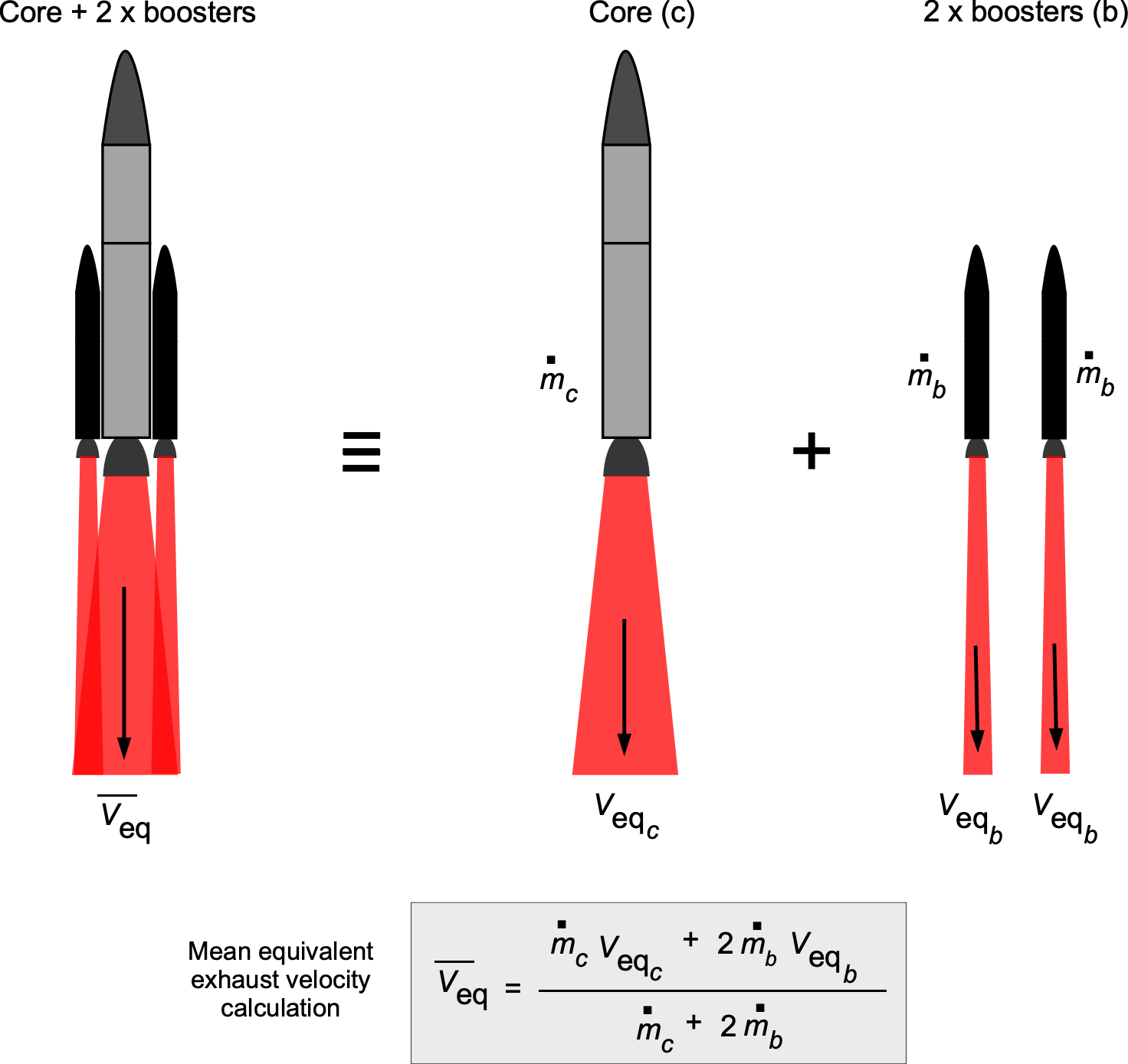
With a parallel staged launch vehicle, there are usually dissimilar rockets and rocket engines burning simultaneously, as shown in the figure below. An example would be the NASA Space Shuttle, which used LH2/LOX for the “core” main engines on the Orbiter, with solid propellant rocket boosters being used to significantly augment the initial launch $\Delta V$ velocity. NASA’s SLS uses the same type of core and booster. Other types of launch vehicles may be configured with different numbers of solid rocket boosters, depending on the payload mass and the desired orbital altitude. An exception is the SpaceX Falcon Heavy, which uses two additional liquid propellant boosters identical to the first (core) stage.

The rocket equation for a core rocket system with one or more boosters can be written as

(47) $\begin{equation*} \Delta V = \overline{V}_{\rm eq} \ln \left( \frac{M_0}{M_b}\right) - g_0 \, t_{b} \end{equation*}$

where $M_0$ is the initial mass (core plus boosters) and $M_b$ is the final mass of the launch vehicle after booster burnout. The average or mean equivalent exhaust velocity, $\overline{V}_{\rm eq}$ , is given by

(48) $\begin{equation*} \overline{V}_{\rm eq} = \frac{ \overbigdot{m}_b \, V_{{\rm eq}_{b}} + \overbigdot{m}_c \, V_{{{\rm eq}_{c}}} }{ \overbigdot{m}_b + \overbigdot{m}_c } \end{equation*}$

where the subscripts $c$ and $b$ refer to the core and the boosters, respectively. The value of $\overbigdot{m}_b$ will be the net mass flow rate of all the boosters. Alternatively, if $\overbigdot{m}$ is the mass flow rate of any one identical booster (there is likely to be more than one booster), then

(49) $\begin{equation*} \overline{V}_{\rm eq} = \frac{ N_b \, \overbigdot{m}_b \, V_{{\rm eq}_{b}} + \overbigdot{m}_c \, V_{{{\rm eq}_{c}}} }{ N_b \overbigdot{m}_b + \overbigdot{m}_c } \end{equation*}$

where $N_b$ is the number of boosters. An illustration of the process for a core rocket system with two boosters is shown in the figure below.

The principle behind the calculation of the equivalent mean velocity.

In this case, the initial mass at the launch point is

(50) $\begin{equation*} M_0 = M_{P_{c}} + M_{P_{b}} + M_{S_{c}} + M_{S_{b}} + M_{L} \end{equation*}$

where $M_{P_{c}}$ and $M_{P_{b}}$ are the propellant masses for the core and the boosters, respectively, $M_{S_{c}}$ and $M_{S_{b}}$ are the structural masses for the core and the boosters, respectively, and $M_{L}$ is the payload mass.

Determining the final burnout mass, $M_b$ , of a launch vehicle with parallel boosters takes further consideration because the core launcher will still have propellant left at booster burnout. Therefore, the final mass at the time of booster burnout, say $t_{b_{0}}$ , can be written as

(51) $\begin{equation*} M_b= \chi M_{P_{c}} + M_{S_{c}} + M_{S_{b}} + M_{L} \end{equation*}$

where $\chi$ is the fraction of propellant mass remaining in the core at booster burnout.

Notice that the mass of propellant, $M_P$ , used in a given time, $t$ , is $M_P = \overbigdot{m} \, t$ , so the mean equivalent exhaust velocity, $\overline{V}_{\rm eq}$ , can also be written as

(52) $\begin{equation*} \overline{V}_{\rm eq} = \frac{ M_{P_{b}} \, V_{{\rm eq}_{b}} + (1 - \chi) \, M_{P_{c}} \, V_{{{\rm eq}_{c}}} }{ M_{P_{b}} + (1 - \chi) M_{P_{c}}} \end{equation*}$

Therefore, the launch of parallel rocket stages can be presented using the sum of pseudo-serial stages, where for stage “0” with the boosters and the core together, then

(53) $\begin{equation*} \Delta V_0 = \overline{V}_{\rm eq} \ln \left( \frac{M_{P_{c}} + M_{P_{b}} + M_{S_{c}} + M_{S_{b}} + M_{L} }{\chi M_{P_{c}} + M_{S_{c}} + M_{S_{b}} + M_{L}}\right) - g_0 \, t_{b_{0}} \end{equation*}$

For stage “1” after booster separation, then the initial mass will be

(54) $\begin{equation*} M_{0_{2}} = \chi M_{P_{c}} + M_{S_{c}} + M_{L} \end{equation*}$

where $\chi$ is the fraction of propellant mass remaining in the core at booster burnout. The final mass after the stage 1 core burns out will be

(55) $\begin{equation*} M_b = M_{S_{c}} + M_{L} \end{equation*}$

where $\chi$ is the fraction of propellant mass remaining in the core at booster burnout.

Therefore, for stage 1, then

(56) $\begin{equation*} \Delta V_1 = \overline{V}_{\rm eq} \ln \left( \frac{ \chi M_{P_{c}} + M_{S_{c}} + M_{L} }{M_{S_{c}} + M_{L} }\right) - g_0 \, t_{b_{1}} \end{equation*}$

The $\Delta V$ values of the remaining stages, $2......N$ , are then calculated as a serial launcher, as before, i.e., the final launch velocity $V_f$ will be

(57) $\begin{equation*} V_f = \Delta V_0 + \Delta V_1 + \Delta V_2 + ......+ \Delta V_N \end{equation*}$

Missiles & Ballistics

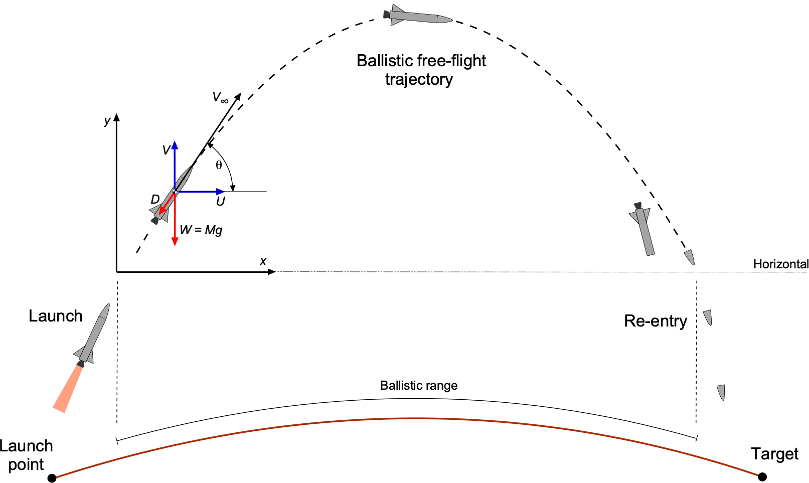
Ballistic trajectories refer to the paths that missiles or artillery projectiles follow from their launch point to their intended targets. Predicting these trajectories is crucial in determining the missile’s flight path, range, and target accuracy. Missile trajectories can vary significantly depending on the type of missile, its intended purpose, the needed range and the altitude it flies to, and the guidance system it uses.

Ballistic missiles follow a trajectory primarily influenced by gravity and the initial launch conditions. They are launched into the atmosphere either vertically or at a steep angle. They then follow a parabolic or elliptical path well into the stratosphere or the edges of space, eventually re-entering the lower atmosphere and impacting their target. Ballistic missiles are known for their high speed and relatively long-range targeting capabilities.

Consider the equations of motion of a missile, as shown in the figure below. For the direction parallel to the flight path, then

(58) $\begin{equation*} M \, a = M \left( \frac{dV_{\infty}}{dt} \right) = T \, \cos \alpha - D - M \, g - M \, g \sin \theta \end{equation*}$

where $M$ is the mass of the missile acting at its center of gravity, and $a$ is its acceleration in the direction of the flight path.

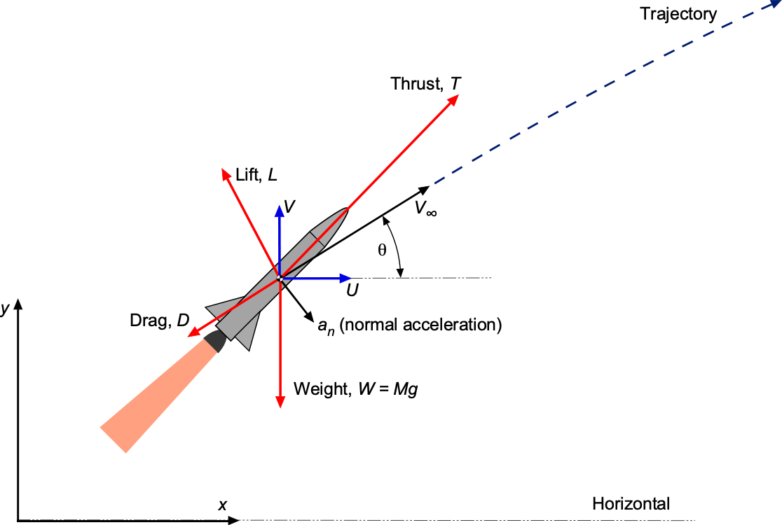
Consideration of the forces acting on a missile in flight can be used to derive its equations of motion.

Similarly, the equation of motion perpendicular to the flight path is

(59) $\begin{equation*} M \, a_n = \frac{M \, V_{\infty}^2}{R} = M \, V_{\infty}^2 \, \left( \frac{d \theta}{ds} \right) = M V_{\infty}^2 \, \left( \frac{d \theta}{dt}\right) \left( \frac{dt}{ds} \right) = M \, V_{\infty} \, \left( \frac{d \theta}{dt} \right) \end{equation*}$

where $s$ is the distance along the flight path, i.e., $s = R \,\theta$ , where $R$ is the instantaneous radius of curvature of the flight trajectory. The second equation of motion is then

(60) $\begin{equation*} M \, v = \frac{d \theta }{dt} = T \sin \alpha + L - M \, g \cos \theta \end{equation*}$

In principle, Eqs. 58 and 60 can be solved to predict the launch trajectory of the missile, much in the manner considered previously using the rocket equation. However, the process is much more complicated than this and requires several more assumptions and approximations to obtain any useful results. Likewise, with the re-entry trajectory, there are many variables to consider, not just limited to simple dynamics and aerodynamics.

In the following more elementary exposition, assume that after the initial launch to high altitude, the rocket engine cuts off so that the thrust, $T$ , is zero, as shown in the figure below. Also, assume that $\alpha = 0$ , so there is no aerodynamic lift.

A missile’s ballistic profile. The actual trajectory will depend on the initial launch conditions, the distance, the altitude of the ballistic profile, and the re-entry profile.

The equations of motion now become

(61) $\begin{eqnarray*} \mbox{$x$-direction:\quad} M \, \overbigddot{x} & = & -D \cos \theta \\[6pt] \mbox{$y$-direction:\quad} M \, \overbigddot{y} & = & -D \sin \theta - M \, g \end{eqnarray*}$

The aerodynamic drag on the missile is given by the standard formula that

(62) $\begin{equation*} D = \frac{1}{2} \varrho_{\infty} \, V_{\infty}^2 \, C_D \, A \end{equation*}$

where the drag coefficient, $C_D$ , is based on the reference area, $A$ , which, by convention, is usually the maximum cross-sectional area of the missile. Let the aerodynamic drag be expressed in the form

(63) $\begin{equation*} D = \mu \, V_{\infty} \, \overbigdot{x} \end{equation*}$

where

(64) $\begin{equation*} \mu = \left[ \frac{ \displaystyle{ \frac{1}{2} \, A \, \varrho_{\infty} \, V_{\infty} C_D}}{\overbigdot{x}}\right]_{\mbox{Mean~value}} \end{equation*}$

where the mean value comprises an average of the aerodynamic drag over the ballistic trajectory. Therefore,

(65) $\begin{equation*} M \, \overbigddot{x} = -\mu \, V_{\infty} \, \overbigdot{x} \, \cos \theta \end{equation*}$

However,

(66) $\begin{equation*} V_{\infty} \, \overbigdot{x} \, \cos \theta = \overbigdot{x} \end{equation*}$

so that

(67) $\begin{equation*} M \, \overbigddot{x} + \mu \, \overbigdot{x}^2 - 0 \end{equation*}$

Letting $\overbigdot{x} = ds/dt = u$ , which seems a reasonable assumption, especially for a long-range ballistic missile, gives

(68) $\begin{equation*} M \left( \frac{d u}{d t} \right) = \mu \, u^2 \end{equation*}$

Separating the variables and integrating them gives

(69) $\begin{equation*} \int \frac{M}{\mu \, u^2} \, du = \int dt \end{equation*}$

This equation has the solution

(70) $\begin{equation*} t = \frac{M}{\mu} \left[ \frac{-1}{u} \right]_{u_0}^{u} = \frac{M}{\mu \, u} - \frac{M}{\mu \, u_0} \end{equation*}$

where $u_0$ is the value of $\overbigdot{x}$ at $t = 0$ . Therefore,

(71) $\begin{equation*} u = \frac{dx}{dt} = \frac{u_0}{1 + \displaystyle{\frac{\mu \, u_0 \, t}{M}}} = \frac{u_0}{1 + \lambda \, t} \end{equation*}$

where $\tau = \mu \, u_0 / M$ . Integrating gives

(72) $\begin{equation*} x = \frac{u_0}{\tau} \ln \left( 1 + \lambda \, t \right) \end{equation*}$

Consider now the equation of motion in the $y$ -direction, which becomes

(73) $\begin{equation*} M \overbigddot{y} = - \mu \, \overbigdot{x} \, \overbigdot{y} - M \, g = -\frac{\mu \, u_0}{1 + \lambda \, t} \overbigdot{y} - M \, g \end{equation*}$

Therefore,

(74) $\begin{equation*} \left( 1 + \lambda \, t \right) g + \lambda \, \overbigdot{y} = -g \left( 1 + \lambda \, t \right) \end{equation*}$

and so

(75) $\begin{equation*} \left( 1 + \lambda \, t \right) = -g \left( t + \frac{\lambda \, t^2}{2} \right) \end{equation*}$

Integrating the preceding equation gives

(76) $\begin{equation*} \left( 1 + \lambda \, t \right) \overbigdot{y} = -g \left( t + \frac{\lambda \, t^2}{2} \right) + v_0 \end{equation*}$

noticing that $\overbigdot{y} = V_0$ at $t = 0$ . By dividing both sides of the foregoing equation by $(1 + \lambda \, t )$ , then

(77) $\begin{equation*} \overbigdot{y} = -\frac{g \, t}{2} - \frac{g}{2 \lambda} + \frac{ v_0 + \displaystyle{ \frac{g}{2 \lambda}}}{1 + \lambda \, t} \end{equation*}$

Integrating yields

(78) $\begin{equation*} y = -\frac{g \, t^2}{4} - \frac{g \, t}{2\lambda} + \left( v_0 - \frac{g}{2 \, \lambda} \right) \frac{ \ln (1 + \lambda \, t)}{\lambda} \end{equation*}$

Therefore, Eqs. 72 and 78 will give the approximate position of the missile’s trajectory in terms of time, $t$ .

Notice that when the aerodynamic drag is small, i.e., the ballistic trajectory is mostly the higher atmosphere or in space, then $\lambda \rightarrow 0$ , and the equations of motion reduce to

(79) $\begin{equation*} \overbigdot{x} = v_0 \mbox{\quad and \quad} x = u_0 \, t = V_0 \cos \theta_0 \, t \end{equation*}$

as well as

(80) $\begin{equation*} \overbigdot{y} = v_0 - g \, t \mbox{\quad and \quad} y = v_0 \, t - \frac{1}{2} g t^2 = V_0 \, \sin \theta_0 \, t - \frac{1}{2} g t^2 \end{equation*}$

Notice that $V_0$ is the initial velocity. These are the classic equations for the parabolic trajectory of any unpowered projectile, such as an artillery shell.

It can be shown that the total flight time, $T_f$ , of the missile or projectile for level ground, i.e., assuming the launch point and target are at the same height, $y = y_0$ , is given by

(81) $\begin{equation*} T_f = \frac{ 2 V_0 \sin \theta_0}{g} \end{equation*}$

where $\theta_0$ is the initial launch angle of elevation of the projectile. The corresponding range, $R_f$ , is

(82) $\begin{equation*} R_f = \frac{V_0^2 \sin 2 \theta}{g} \end{equation*}$

The maximum range occurs when $\theta_0$ = 45 $^{\circ}$ , i,e., $\sin 2\theta_0 = 1$ .

These preceding equations, collectively, are sometimes referred to as the Laws of Ballistics or the Artilleryman’s Range Equations. However, if the variation of $g$ is accounted for during high-altitude flight using the inverse-square law of gravitational attraction, then the trajectory will be elliptic. The effect would be to increase slightly the range of a high-altitude projectile.

Summary & Closure

Payloads that must be launched into space vary widely, including communication satellites, weather satellites, scientific instruments, and planetary exploration probes. Payload mass and size are crucial considerations when configuring a launch vehicle. Heavier payloads and higher orbital altitudes require larger and more powerful rockets. For low Earth orbit (LEO) missions, where satellites like Earth observation satellites or communication satellites are deployed, the launch vehicle needs less energy than missions going to geostationary orbit or interplanetary destinations.

Companies like SpaceX and Blue Origin have been pioneering the development of new rocket technologies, which have transformed the space industry. SpaceX has developed crewed spacecraft, like Crew Dragon, to transport astronauts to and from the International Space Station. Commercial companies are launching satellites for communication and Earth observation and are actively working on making space tourism a reality. This could potentially open up new opportunities and industries in the future. Ongoing research and development in propulsion technologies continue to influence the design of future launch vehicles, making them more efficient and capable.

5-Question Self-Assessment Quickquiz

For Further Thought or Discussion

Consider a staged vehicle for which all $V_{\rm eq}$ values are the same. How can $\Delta V$ be maximized?
How does a rocket navigate and change its course during flight?
What is the role of aerodynamics in rocket design?
How do scientists and engineers calculate the optimal launch trajectory for a rocket?
What are the challenges of reusing rockets, and why is rocket reusability important?
Can you name some famous rockets and their notable achievements?
How has rocket technology evolved, and what are the prospects for rocketry?

Other Useful Online Resources

To learn more about rockets, launch vehicles, and other spacecraft, check out these helpful online resources:

An article on the history of rockets by NASA
Great video: The Evolution of Space Rockets.
The U.S.’s first person in space, Alan Shepard, launches on a Mercury Redstone rocket.
Saturn V: The rocket that took humans to the Moon – The Saturn V Story.
Experience the flight of Apollo 11.
STS-134 – The final launch of the Space Shuttle Endeavour.
Artemis I Launch to the Moon – Official NASA Broadcast – Nov. 16, 2022.
First test flight of the SpaceX Falcon Heavy.
SpaceX Falcon Heavy launches the NASA Psyche – see video here.
SpaceX Starship SN10 launch and landing – see video here.
Blastoff! Blue Origin launches 33 payloads.

License

Icon for the Creative Commons Attribution-NonCommercial-NoDerivatives 4.0 International License

Introduction to Aerospace Flight Vehicles Copyright © 2022, 2023, 2024 by J. Gordon Leishman is licensed under a Creative Commons Attribution-NonCommercial-NoDerivatives 4.0 International License, except where otherwise noted.