Takeoff & Landing Performance

J. Gordon Leishman

doi:https://doi.org/10.15394/eaglepub.2022.1066.n40

41 Takeoff & Landing Performance

Introduction

The ability for airplanes to operate adequately and safely from airports requires that they be suitably designed to have acceptably low takeoff and landing distances, plus some safety margins. The principal interest is to have sufficient runway length to the liftoff point (at a given flight weight and takeoff density altitude), as well as to clear any obstacles (e.g., buildings or terrain) from the initiation of the takeoff roll. It must also be ensured that the takeoff airspeeds are low enough that the pilot can abort the takeoff in an emergency and still have sufficient runway length to decelerate safely to a complete stop. As shown in the photograph below, the takeoff process looks almost effortless when watching a modern airliner climb away from the runway. However, substantial amounts of thrust and power are required to perform this aeronautical feat. Also, the airplane must be flown at a precise airspeed to maximize its angle of climb and/or rate of climb.

The best angle of climb will be used to clear any ground obstacles, followed by building up airspeed to climb at the best rate to the initial cruise altitude.

The takeoff distance and airspeed at which the airplane can safely fly can be significantly reduced using flaps and other high-lift devices such as slats. An optimum flap/slat setting will minimize the takeoff distance and maximize the initial rate of climb. For multi-engine airplanes, adequate single-engine out (one engine inoperative or OEI) performance is also essential. The loss of an engine at a critical point in the takeoff run is an emergency and will require the airplane to either stop in the remaining runway length or to continue the takeoff and climb on the remaining engine(s). For a landing, the airplane must also be able to touch down on the runway at the lowest possible airspeed and stop well within the available runway length. To this end, flaps, spoilers, reverse thrust (if available), and good wheel brakes are all important.

Learning Objectives

Understand the factors affecting the takeoff performance of an airplane.
Appreciate the factors that can affect an airplane’s landing and stopping distances.
Use appropriate equations to estimate an airplane’s takeoff and landing distances.

Takeoff Performance

During a takeoff maneuver, the airplane is in accelerated motion and experiences a continuously increasing airspeed. Finally, sufficient airspeed will be reached for the airplane to fly after covering a certain runway length, called the liftoff or “unstick” point. It is essential to keep the airplane on a straight course down the runway, which is done using nose-wheel steering and then rudder control as airspeed builds. Then, as illustrated in the figure below, the pilot will pull back on the elevator control to increase the pitch attitude, and the airplane creates enough lift to transition into flight and climb away from the ground. In the early stages of flight, the airplane is held at a moderate climb rate and allowed to accelerate until the best climbing rate is reached. The takeoff maneuver is relatively routine, but pilots always need to be prepared for unexpected emergencies, such as the loss of an engine or other mechanical malfunction.

The total takeoff distance is measured in terms of a ground roll, some short transition distance, and some additional distance needed to pass over an FAA-mandated 50-ft high obstacle.

The total takeoff distance for the airplane at a given weight and operating density altitude is determined from the sum of three parts:

The ground roll to the point where the airplane reaches a safe airspeed to fly, called the liftoff distance.
The transition distance is when the pilot pulls back on the stick (or yoke) and lifts the airplane’s nose to a climbing attitude. The lift builds up on the wing, and the airplane leaves the runway.
The extra distance for the airplane needed to climb and pass over a fictitious 50-ft (15-m) high obstacle.

The fictitious 50-ft (15-m) high obstacle requirement recognizes that most runways inevitably have trees or some structure(s) at their ends. FAA certification of airplanes per the FAA regulations (FARs) requires that the reported takeoff distances factor in this extra margin of safety to prevent pilots from underestimating the needed runway lengths – see CFR §23.2115 and CFR §25.105 and onward.

Takeoff Analysis

Estimates of an airplane’s ground roll to the point of liftoff and total takeoff distances can be determined using the basic principles of dynamics and aerodynamics. However, the solution of the resulting equations will usually require numerical integration, not least because the exact value of propulsive thrust is not necessarily known a priori; this latter issue also depends on whether it is a jet or a propeller airplane. In addition, other factors, such as the rolling friction of the wheels on the runway, may not be known precisely, although estimates can be made for different runway surfaces, including both dry and wet. Nevertheless, reasonable estimates of the liftoff and takeoff distance(s) are possible with some assumptions. These estimates can help engineers evaluate the factors influencing the needed runway lengths for a new airplane.

Consider an airplane of mass $M$ ( $=W/g$ ) acted upon by a thrust $T$ from the propulsion system, as shown in the figure below. There will also be a rolling resistance force, which depends on the coefficient of friction $\mu_r$ from the wheels on the runway surface.

The forces acting on an airplane during the takeoff roll. Rolling friction depends on the nature of the runway surface and whether it is dry or wet.

At the beginning of the ground roll, lift and drag are zero because the dynamic pressure is still zero (assuming no winds). Rolling friction forces progressively decrease as the lift develops on the wings and becomes zero at the liftoff point. As soon as the landing gear is retracted, the airplane’s drag decreases, and the airplane establishes its initial climb out.

The amount of rolling resistance $R$ depends on the net vertical force on the wheels, which is given by

(1) $\begin{equation*} R = \mu_r ( W - L) \end{equation*}$

where $L$ is the lift produced and $W$ is the aircraft’s weight. For a dry, paved runway, the coefficient of friction, $\mu_r$ , is about 0.02. This value may increase to as much as 0.1 for a wet runway, so engineers and pilots must know that a wet runway can significantly increase takeoff distances. The standard aerodynamic formula gives the lift on the wing as

(2) $\begin{equation*} L = \frac{1}{2} \varrho_{\infty} \, V_{\infty}^2 \, S \, C_L \end{equation*}$

There is also an increasing drag on the airplane as it builds up airspeed, which can be written in the standard way as the sum of non-lifting and lifting components, i.e.,

(3) $\begin{equation*} D = \frac{1}{2} \varrho_{\infty} V_{\infty}^2 S C_D = \frac{1}{2} \varrho_{\infty} V_{\infty}^2 S \left( C_{D_{0}} + \phi \frac{{C_L}^2}{\pi \, AR \, e} \right) \end{equation*}$

In this case, the factor $\phi$ accounts for the runway’s proximity on the airplane’s induced drag, i.e., the so-called “ground effect,” the physics of which is explained later in more detail. While various equations have been used to represent this ground effect or “ $\phi$ factor,” one standard approximation is to use

(4) $\begin{equation*} \phi = \frac{16(h/b)^2}{1 + (16h/b)^2} \end{equation*}$

where $h$ is the height of the wing above the runway, and $b$ is the wing span. The phenomenon of ground effect is important near the runway (where $\phi$ may be between 0.5 and 0.7 depending on the airplane), but $\phi$ increases quickly to unity as $h$ increases to one or more wing spans above the runway.

Therefore, the net (accelerating) force on the airplane will be

(5) $\begin{equation*} T - R - D = T - \mu_r ( W - L) - D = F \end{equation*}$

where $T$ is the thrust, $R$ is the rolling resistance, and $D$ is the drag. The airspeed increases because the thrust exceeds the total friction and drag forces during the takeoff roll. The resulting acceleration of the airplane, $a$ , will be

(6) $\begin{equation*} a = \frac{dV_{\infty}}{dt} = \frac{F}{M} = \frac{ F g}{W} = \frac{\big(T - \mu_r ( W - L) - D \big) g}{W} \end{equation*}$

noting again that $W = M g$ , so $M = W/g$ . Therefore, after a time $t$ from the start of the takeoff roll, the airspeed will be

(7) $\begin{equation*} V_{\infty} = \int_0^t \left( \frac{F}{W} \right) \, g \, dt \end{equation*}$

the resultant force $F$ depends on engine thrust, rolling friction, and drag, which depend on airspeed, $V_{\infty}$ .

Equation 7 is the first integration required to estimate the takeoff distance. A second integration, therefore, gives the distance traveled during the acceleration to the liftoff (LO) point, i.e.,

(8) $\begin{equation*} s_{\textnormal{\tiny LO}} = \int_0^t V_{\infty} \, dt \end{equation*}$

which can be used to help solve for the takeoff run and liftoff distance if the airspeed at which the airplane will fly is known (or assumed). Alternatively, if the maximum lift coefficient of the wing is known (in its takeoff configuration), then the corresponding takeoff airspeed can be determined.

Approximate Solutions

There are no closed-form solutions to the preceding equations (Eq. 7 and 8) for the liftoff distance unless assuming particular assumptions and approximations. Examples include constant or diminishing thrust from the propulsion system. To this end, the equation of motion as given by Eq. 6 can also be written as

(9) $\begin{equation*} \frac{1}{g} \left( \frac{dV_{\infty}}{dt} \right) = \left( \frac{T}{W} - \mu_r \right) - \frac{1}{W} \left( D - \mu_r L \right) \end{equation*}$

or

(10) $\begin{equation*} \frac{1}{g} \left( \frac{dV_{\infty}}{dt} \right) = \left( \frac{T}{W} - \mu_r \right) - \frac{\displaystyle{ \frac{1}{2} \varrho_{\infty} V_{\infty}^2 S }}{W} \bigg( C_D - \mu_r \, C_L \bigg) \end{equation*}$

Assume that the thrust can be written as $T = T_0 - k V_{\infty}^2$ , where $k$ is a constant, i.e., the thrust decreases with increasing airspeed. In this case, then

(11) $\begin{equation*} \frac{1}{g} \left( \frac{dV_{\infty}}{dt} \right) = \left( \frac{T_0}{W} - \mu_r \right) - \frac{ V_{\infty}^2}{W} \bigg(\frac{1}{2} \varrho_{\infty} S \left( C_D - \mu_r \, C_L \right) + k \bigg) \end{equation*}$

which can be written as

(12) $\begin{equation*} \frac{dV_{\infty}}{dt} = A - B V_{\infty}^2 \end{equation*}$

where

(13) $\begin{equation*} A = \left( \frac{T_0}{W} - \mu_r \right) \, g \end{equation*}$

and

(14) $\begin{equation*} B = \frac{g}{W} \bigg( \frac{1}{2} \varrho_{\infty} S \left( C_D - \mu_r \, C_L \right) + k \bigg) \end{equation*}$

Separating the variables and integrating them gives

(15) $\begin{equation*} \int \frac{dV_{\infty}}{A - B V_{\infty}^2} = \int dt \end{equation*}$

which has the solution

(16) $\begin{equation*} t = \left( A \, B \right)^{-1/2} \tanh^{-1} \left( V_{\infty} \sqrt{\frac{B}{A} }\right) \end{equation*}$

where $\tanh$ is the hyperbolic tangent. Therefore, the time taken on the ground run to the point of liftoff (LO) may be obtained by replacing $V_{\infty}$ by the airspeed at liftoff, which must be estimated. Normally, this latter airspeed is defined as 1.2 times the stalling airspeed of the airplane in the takeoff configuration.

The corresponding length of the ground run to the liftoff point can also be estimated. In this case, the equation of motion can be written as

(17) $\begin{equation*} T - \mu_r ( W - L) - D = \left( \frac{W}{g} \right) V_{\infty} \left( \frac{ d V_{\infty} }{ds} \right) \end{equation*}$

where $s$ is distance. This equation leads to

(18) $\begin{equation*} V_{\infty} \frac{ d V_{\infty} }{ds} = A - B V_{\infty}^2 \end{equation*}$

Separating the variables and integrating them gives

(19) $\begin{equation*} \int \frac{ V_{\infty} d V_{\infty} }{A - B V_{\infty}^2} = \int ds \end{equation*}$

which has solution

(20) $\begin{equation*} s = -\frac{1}{2B} \ln \left( A - B V_{\infty}^2 \right) + C \end{equation*}$

At $s = 0$ then $V_{\infty} = 0$ , so

(21) $\begin{equation*} C = \frac{1}{2B} \ln A \end{equation*}$

Therefore, for these assumptions, the liftoff distance, $s_{\textnormal{\tiny LO}}$ , can be expressed as

(22) $\begin{equation*} s_{\textnormal{\tiny LO}} = \frac{1}{2B} \bigg( \ln A - \ln \left(A - B V_{\infty}^2 \right) \bigg) = \frac{1}{2B} \ln \left( \frac{A}{A - B V_{\infty}^2} \right) \end{equation*}$

Other Approximations

Other assumptions can be used to solve the takeoff equations of motion. However, one established approximation for estimates of the “lift-off” (LO) distance, $s_{\textnormal{\tiny LO}}$ , for aircraft design purposes, is given by

(23) $\begin{equation*} s_{\textnormal{\tiny LO}} = \frac{1.44 \, W^2}{g \, \varrho_{\infty} \, S \, C_{L_{\rm max}} ( T - \bigg( D + \mu_r (W - L) \bigg)_{\rm av}} \end{equation*}$

where the average net resistive force from the drag and rolling friction is given by

(24) $\begin{equation*} \bigg( D + \mu_r (W - L) \bigg)_{\rm av} = \bigg( D + \mu_r (W - L) \bigg)_{0.7 V_{\textnormal{\tiny LO}}} \end{equation*}$

The term $0.7 V_{\textnormal{\tiny LO}}$ means that this previous quantity is evaluated at 70% of the liftoff airspeed, $V_{\textnormal{\tiny LO}}$ , which can be determined in terms of the estimated stall airspeed using

(25) $\begin{equation*} V_{\textnormal{\tiny LO}} = 1.2 \, V_{\rm stall} = 1.2 \sqrt{ \frac{2 W}{\varrho_{\infty} \, S \, C_{L_{\rm max}}}} \end{equation*}$

The factor 1.2 is included to give some margin for safety between the stall airspeed and the flying airspeed. Of course, this analysis is predicated on a knowledge of $C_{L_{\rm max}}$ for the wing, a complication being that the wing operates in ground effect, as previously discussed, so this value can only be estimated.

Further simplifications can be made to such analyses, such as the drag and rolling friction force is much less than the thrust force (again, this is reasonable for a high-performance airplane) to get

(26) $\begin{equation*} s_{\textnormal{\tiny LO}} = \frac{1.44 \, W^2}{g \, \varrho_{\infty} \, S \, C_{L_{\rm max}} \, T} \end{equation*}$

which depends only on thrust, $T$ , so this latter equation provides a simple basis for establishing the primary effects that can be expected to affect the takeoff distance.

Effects of Flaps and Slats

From the preceding, it is clear that both the takeoff distances are affected by the maximum lift coefficient attainable by the wing, i.e., by the value of $C_{L_{\rm max}}$ , as shown in the figure below. This reason is why flaps and slats are used on airplanes, flaps alone being more common on low-performance airplanes and both flaps and slats being used on higher-performance airplanes such as airliners. Flaps can also be used to increase the wing area if they are designed to move aft and deflect downward. Both flaps and slats are mechanical devices that the pilot operates as appropriate to the flight condition.

The maximum attainable lift coefficient depends on whether the flaps or slats are retracted or deployed. If they are retracted, the wing is said to be in its “clean” configuration.

Slats, however, are usually found only on higher-performance and heavier airplanes. A slat is like a small secondary airfoil at the wing’s leading edge. When the slats are deployed, air flows through the gap and over the top surface of the airfoil, and the resulting flow helps to energize the boundary layer and delay the onset of flow separation and stall. The wing can then be flown at a higher angle of attack before stall with a commensurate increase in $C_{L_{\rm max}}$ . The reduction in takeoff distances, as well as landing distances using high-lift devices, is generally significant.

The reduction in takeoff distances using high-lift devices is generally significant.

Numerical Solutions

The equations of motion can also be used to numerically solve the takeoff distance problem using more realistic assumptions, such as the propulsive thrust characteristics for specific engines. Airplane manufacturers carefully do these calculations for different takeoff weights, atmospheric conditions (i.e., different density altitudes), runway conditions, and winds and then verify the results using actual flight tests with the airplane. Notice that the same aircraft type may be available from the manufacturer with different engines, so the process must be completed for each aircraft type and engine combination.

Representative results are shown in the figure below, obtained by numerical integration, time step by time step, and using more realistic assumptions. These types of calculations can be repeated for cases of single-engine failure (with multi-engine aircraft) before the point of takeoff, i.e., by reducing the available thrust by half for a twin-engine aircraft. In this case, which is called a rejected takeoff, the required stopping distance on the remaining runway must be calculated using reverse thrust (if available) and braking.

Representative results for the solution to the equations of motion for a takeoff maneuver.

Effects of Winds

The effects of winds on the takeoff distance can be estimated by replacing $V_{\infty}$ by $V_{\infty} - V_w$ , where $V_w$ is the headwind component. Therefore, Eq. 2 can be replaced by

(27) $\begin{equation*} L = \frac{1}{2} \varrho_{\infty} \left( V_{\infty} + V_w \right)^2 S C_L \end{equation*}$

which will also apply to the equations following Eq. 2. Therefore, with a headwind, the wing lift will build up quicker, and flying conditions will be reached much sooner, reducing the ground run and takeoff distance. Notice also that with a tailwind, it will take much longer to reach flying conditions, and the needed runway lengths may be larger than those available. Tailwind components are particularly critical at “hot and high” conditions where the air density, $\varrho_{\infty}$ , may be substantially less than a sea level.

Takeoff Charts

At the end of performance flight testing, the airplane’s takeoff performance results are generalized for standard and non-standard ISA conditions and included in the flight performance charts for use by the pilots. The figure below shows a simple example for a general aviation airplane. These charts are mainly used for flight planning.

An example of a takeoff distance chart for an airplane as would be included in the operating manual.

From knowledge of the airplane’s weight, the prevailing values of pressure altitude (as measured on the altimeter), outside air temperature, and the winds, the pilot can use this type of chart to estimate the airplane’s anticipated takeoff distance. Remember that the basis of this chart is modeling and engineering data verified by testing. While the chart looks complicated at first glance, pilots soon learn to make reasonable estimates for their takeoff performance. Notice again the significant effect of airplane weight on the takeoff distance and the impact of increasing temperature above ISA standard conditions, i.e., the impact of increasing density altitude. Notice that, as previously discussed, a headwind can notably reduce the takeoff distances; the chart also suggests that taking off with a tailwind is never a good idea because takeoff distances can be increased significantly.

Summary: Factors Affecting Liftoff Distances

In summary, regardless of the assumptions and/or approximations, the preceding results show the following outcomes:

The liftoff distance increases with the square of the airplane’s weight, meaning that if the weight is increased by 50%, the runway needed will increase by over twice.
The liftoff distance increases with decreasing air density (i.e., density altitude), explaining why airplanes take significantly more runway length on hot days or when operating out of airports at high elevations.
The liftoff distance is reduced by using more wing area and/or by increasing $C_{L_{\rm max}}$ , which is why some flaps are used during takeoff but not so much as to increase the drag substantially. Note: Some military airplanes use rocket devices to increase net thrust when the runway is short. Catapults onboard an aircraft carrier provide augmented force where flying airspeed must be attained in a matter of seconds.
Winds can decrease or increase takeoff distances. If there is a headwind or headwind component, takeoff distances will be reduced. If there is a tailwind or tailwind component, takeoff distances can increase considerably.

Worked Example #1 – Estimating takeoff distance

A small jet aircraft has a ramp weight of 6,600 lb, and its engines have a maximum thrust of 1,200 lb. The drag polar of the aircraft in the takeoff configuration is $C_D = 0.03 + 0.055 \, C_L^2$ . The wing area is 160 ft². If the winds are calm, what will be the estimated takeoff airspeed and takeoff distance? Assume that the wing stall lift coefficient, $C_{L_{\rm max}}$ , is 1.6 and that the wing operates at $C_L = 0.4$ during the takeoff roll. Also, assume that the runway is dry and the aircraft on the runway is at MSL ISA conditions.

The stall airspeed of the aircraft in the takeoff configuration can be estimated using

$V_{\rm stall} = \sqrt{ \frac{2 W}{\varrho_{\infty} \, S \, C_{L_{\rm max}}}}$

For this aircraft, then

$V_{\rm stall} = \sqrt{ \frac{2 \times 6,600 }{0.002378 \times 160.0 \times 1.6} } = 140.4~\mbox{ft/s} \approx 83.2~\mbox{kts}$

The lift-off airspeed will be 1.2 times the stall airspeed, so

$V_{\textnormal{\tiny LO}} = 1.2 \, V_{\rm stall} = 1.2 \times 140.4 = 168.5~\mbox{ft/s} \approx 100~\mbox{kts}$

To find the takeoff distance, the average net resistive force, $R_{\rm av}$ , from the drag and rolling friction can be calculated using

$R_{\rm av} = \bigg( D + \mu_r (W - L) \bigg)_{0.7 V_{\textnormal{\tiny LO}}}$

where $0.7 V_{\textnormal{\tiny LO}}$ means that this previous quantity is evaluated at 70% of the liftoff airspeed, $V_{\textnormal{\tiny LO}}$ . The lift on the aircraft at $0.7 V_{\textnormal{\tiny LO}}$ will be

$\begin{eqnarray*} L & = & \frac{1}{2} \varrho_{\infty} \left( 0.7 V_{\textnormal{\tiny LO}} \right)^2 S \, C_L \\ & = & 0.5 \times 0.002378 \times \left( 0.7 \times 168.5 \right)^2 \times 160.0 \times 0.4 = 1,058.7~\mbox{lb} \end{eqnarray*}$

The corresponding drag coefficient at $C_L$ = 0.4 during the takeoff roll will be

$C_D = 0.03 + 0.055 \, C_L^2 = 0.03 + 0.055 \times 0.4^2 = 0.0388$

and so the drag on the aircraft at $0.7 V_{\textnormal{\tiny LO}}$ will be

$\begin{eqnarray*} D & = & \frac{1}{2} \varrho_{\infty} \left( 0.7 V_{\textnormal{\tiny LO}} \right)^2 S \, C_D \\ & = & 0.5 \times 0.002378 \times \left( 0.7 \times 168.5 \right)^2 \times 160.0 \times 0.0388 = 102.7~\mbox{lb} \end{eqnarray*}$

The runway is dry, so $\mu_r$ = 0.02. Therefore, the average resistive force is

$R_{\rm av} = D + \mu_r (W - L)]_{0.7 V_{\textnormal{\tiny LO}}} = 102.7 + 0.02 \left( 6,600 - 1,058.7 \right) = 213.5~\mbox{lb}$

$s_{\textnormal{\tiny LO}} = \frac{1.44 \, W^2}{g \, \varrho_{\infty} \, S \, C_{L_{\rm max}} ( T - \bigg( D + \mu_r (W - L) \bigg)_{\rm av} )} = \frac{1.44 \, W^2}{g \, \varrho_{\infty} \, S \, C_{L_{\rm max}} ( T - R_{\rm av} )}$

Substituting the numerical values gives

$s_{\textnormal{\tiny LO}} = \frac{1.44 \times 6,600^2}{32.17 \times 0.002378 \times 160.0 \times 1.6 \times \left( 1,200 - 213.5 \right)} = 3,247~\mbox{ft}$

Landing Performance

As they say, what goes up must come down, so eventually, the airplane needs to come in for a landing. Setting up the approach toward the runway requires the pilot to reduce power and decrease airspeed to produce a controlled rate of descent. The flaps and slats (if any) will be deployed, and the landing gear (if retractable) will be extended, as shown in the photograph below. The rate of descent is controlled by engine power adjustments and the pitch attitude using the elevators. The approach is continued until the aircraft is close to the ground, where the pilot flares by pulling back on the controls (up elevator) and bringing the aircraft in a slightly nose-high attitude before the wheels contact the runway at the lowest possible rate of descent.

An airliner configured for landing with flaps and slats deployed and the gear down.

The final landing maneuver is typically performed at or near the lowest possible airspeed, keeping the landing distance as short as possible. This situation is where the application of wing flaps and slats (if the airplane has them) is advantageous because their use can increase the wing’s maximum lift coefficient by up to a factor of approximately two. After landing, the pilot uses the rudder to keep the airplane on a straight course down the runway and then nose-wheel steering as airspeed bleeds off. Reverse thrust, if available, can be used to shorten the landing distance by over 50%.

Analysis

The figure below shows the forces acting on an airplane during the landing rollout; they are the same as during the takeoff, except that the thrust will now be zero or negative (i.e., the use of reverse thrust, if available). The wing’s drag coefficient will dramatically increase by deflecting the flaps downward and using spoilers. The rolling friction is much greater if the brakes are applied, with $\mu_r = 0.4$ being a typical value for braking on a dry paved runway. Brakes may only be applied for part of the landing distance, depending on the pilot’s discretion and the available runway length. Spoilers on the wings are used to decrease the lift on the wings and increase the weight onto the wheels to increase the rolling friction and braking action during the landing roll.

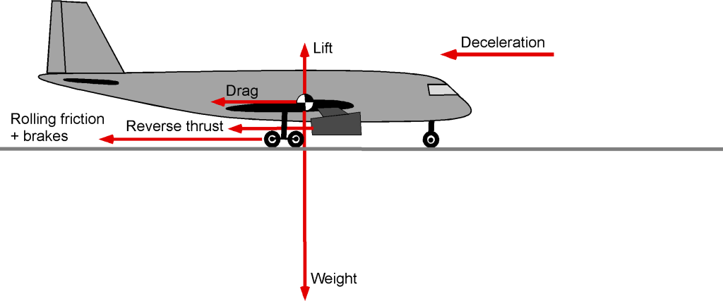
When the airplane touches down, engine thrust is brought to idle by the pilot, or with most jet and turboprop airplanes, negative or “reverse” thrust can be produced using thrust reversers or reverse (i.e., negative) pitch propellers. Because of the high landing airspeeds of many military airplanes, some may need to use a parachute deployed during the landing run. Aircraft carriers bring airplanes to a quick stop by engaging an arrester cable across the flight deck. However, this does impose large structural loads on the airplane and uncomfortably high decelerations on the pilot.

The same equations as for the takeoff apply here, but now $T = 0$ if not a negative value, i.e.,

(28) $\begin{equation*} a = \frac{dV_{\infty}}{dt} = \frac{(-\mu_r ( W - L) - D) g}{W} \end{equation*}$

the net negative force confirming a deceleration. If the lift on the wings can be dumped by using wing spoilers, then it is possible to assume $L = 0$ (or perhaps just a significantly smaller value than $W$ ), and so the weight of the airplane is entirely on its wheels, and the deceleration will be

(29) $\begin{equation*} a = \frac{dV_{\infty}}{dt} = \frac{(- \mu_r W - D) g}{W} = \frac{ F \, g}{W} \end{equation*}$

The corresponding reduction in airspeed can be calculated using

(30) $\begin{equation*} V_{\infty} = \int_0^t \left( \frac{F}{W} \right) \, g\, dt \end{equation*}$

where $t = 0$ occurs at the touchdown with the second integration giving the actual landing distance, i.e.,

(31) $\begin{equation*} s_{\textnormal{\tiny L}} = \int_0^t V_{\infty} \, dt \end{equation*}$

Approximations

As with the takeoff problem, simplified solutions for landing distance are possible with certain assumptions and approximations. In this case, $\mu_R$ will be greater because of the application of wheel brakes. One result often used for aircraft design purposes is that

(32) $\begin{equation*} s_{\textnormal{\tiny L}} = \frac{1.69 \, W^2}{g \varrho_{\infty} \, S \, C_{L_{\rm max}} \bigg( D + \mu_r (W - L) \bigg)_{0.7 V_{\textnormal{\tiny T}} }} \end{equation*}$

where

(33) $\begin{equation*} V_{\textnormal{\tiny T}} = 1.3 \, V_{\rm stall} = 1.3 \sqrt{ \frac{2 W}{\varrho_{\infty} \, S \, C_{L_{\rm max}}}} \end{equation*}$

with the factor 1.3 being included in this case to give a good margin for safety above the stall airspeed as well as for ground effect. In the landing configuration, flaps or other high-lift devices will increase the value of $C_{L_{\rm max}}$ over the attainable value in the takeoff configuration.

Effects of Winds

The effects of winds on the landing distances can be estimated in a manner similar to takeoff distances. With a headwind, the aircraft’s speed relative to the runway will be reduced, with corresponding reductions in landing distance. As with takeoff distances, tailwind components will markedly increase landing distances. Again, such effects are particularly critical at “hot and high” conditions where the air density, $\varrho_{\infty}$ , may be substantially less than at sea level.

Landing Charts

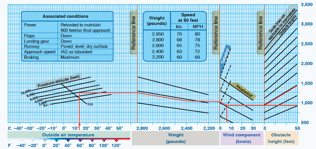
As with the takeoff performance, the preceding integrations would be performed numerically (with certain assumptions), and the results for the estimated landing distances would be verified by flight testing at different airplane weights and atmospheric conditions, perhaps also with different runway conditions, i.e., dry versus wet. Along with the takeoff distance, the results will eventually be included in the flight performance charts for the airplane for use by the pilots; a simple example is shown below. Again, this chart type will be used mainly for flight planning, e.g., to determine whether the destination airfield has sufficient runway lengths.

An example of a landing distance chart for an airplane that would be included in the flight manual.

Landing distances will also depend on the square of the airplane’s weight, so a heavier airplane will require much more runway length. Distances will also increase at lower air densities, i.e., higher density altitudes, which means higher elevation airports and hotter conditions relative to ISA. Again, the importance of high lift devices becomes apparent, which will increase the $C_{L_{\rm max}}$ of the wing in the landing configuration to reduce both landing airspeeds and required runway distances.

Remember that the previous methods and results are mathematical approximations, and better estimates of the takeoff and landing distances will require numerical solutions. Airplane manufacturers always do many flight tests to verify these numerical predictions before including the final takeoff and landing performance results in the flight manuals.

Summary: Factors Affecting Landing Distances

In summary, regardless of the assumptions and/or approximations, the preceding results show the following outcomes:

The landing distance increases with the square of the airplane’s weight, meaning that if the weight is increased by 50%, the runway needed to kand and stop will increase by over twice.
The landing distance increases with decreasing air density (i.e., density altitude), explaining why airplanes will need more runway length on hot days or when operating out of airports at high elevations.
The landing distance is reduced by using more wing area and/or increasing $C_{L_{\rm max}}$ . Full flaps and other high-lift devices will be deployed to minimize the landing distance.
If there is a headwind or headwind component, landing distances will be reduced. If there is a tailwind or tailwind component, landing distances can increase considerably to the point that the available runway lengths may be insufficient.

Physics of “Ground Effect”

As previously mentioned, ground effect is important in establishing an airplane’s takeoff and landing distances. The physics of why this occurs requires further explanation. When an airplane nears the ground, the three-dimensional flow pattern around its wings changes, primarily affecting the wing tip vortex formation and their positions relative to the wing. The consequence of this behavior is to alter the downwash field over the wing and its induced drag, as illustrated in the figure below.

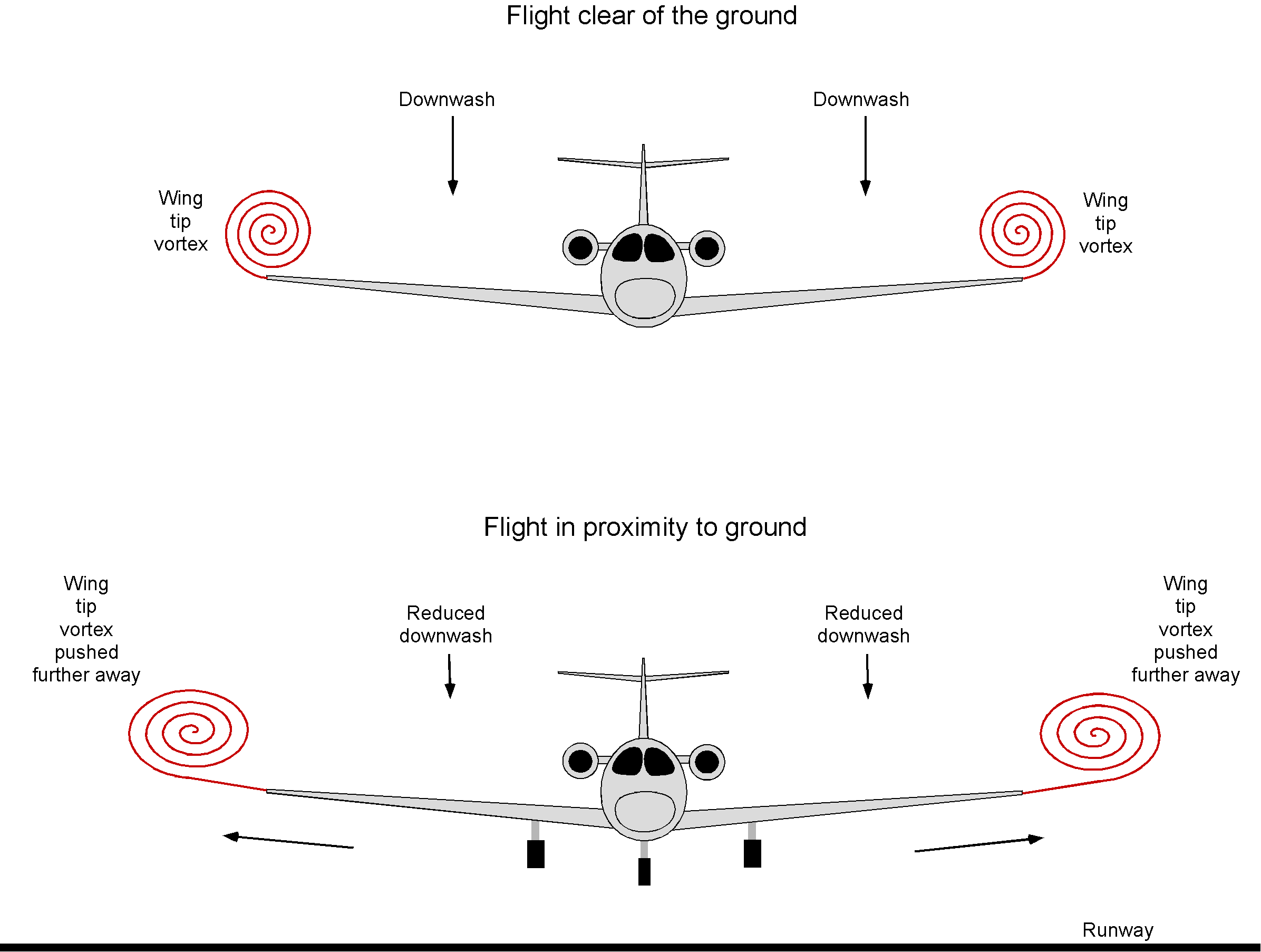
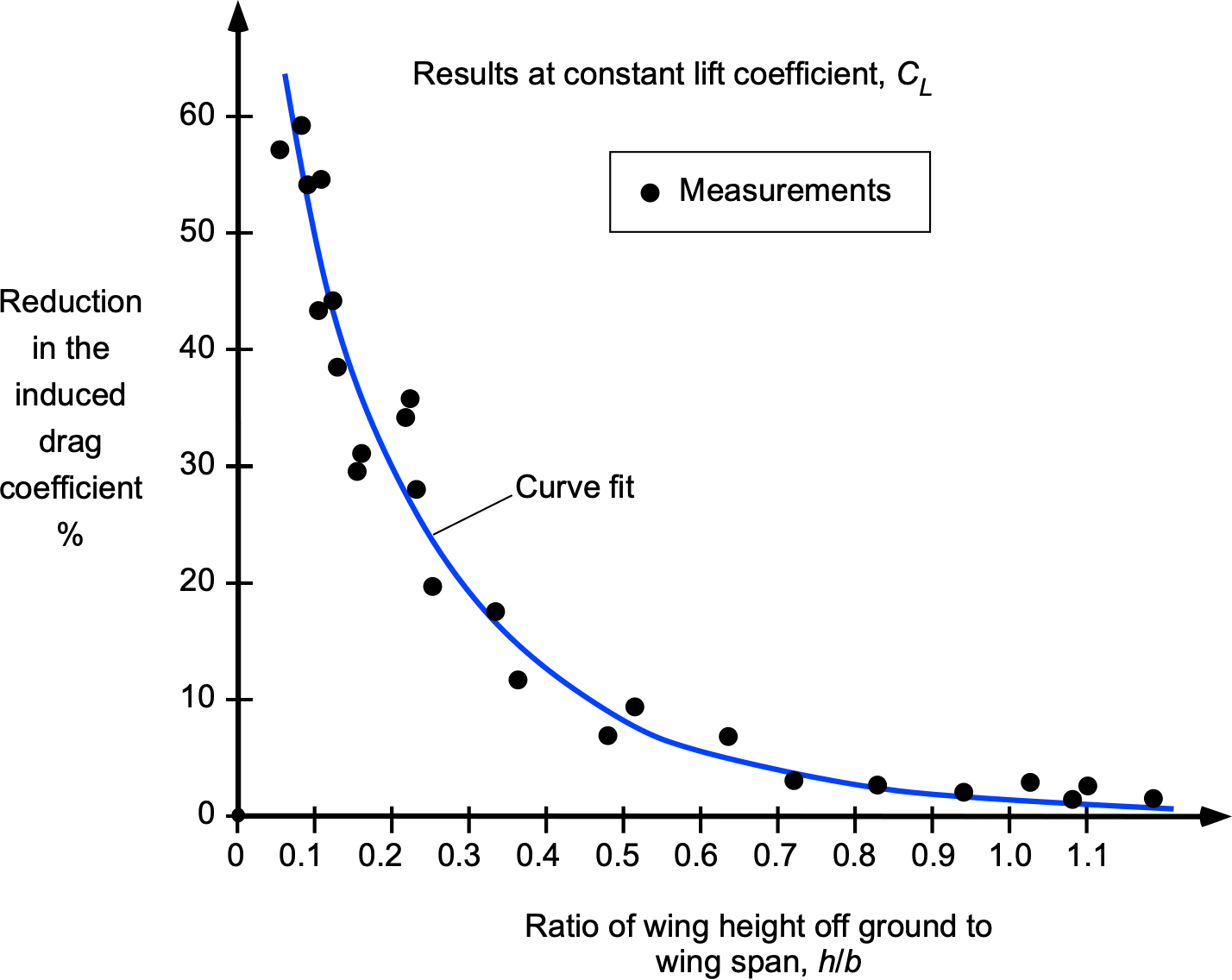
The “ground effect” physics manifests primarily as a decrease in downwash over the wing and a decrease in the induced drag whenever the wing is within about one wing span of the ground.

The primary consequence of the “ground effect” is a decrease in the induced component of drag whenever the wing is within about one wing span of the ground, although some increase in lift is also produced. The consequence is that in ground effect operation, the wing appears aerodynamically to have a higher aspect ratio. Ground effect is often particularly noticeable to a pilot during landing, wherein the landing flare, the airplane may seem to “float” just above the runway for some distance before the wheels touch down. While there may be some alteration in the aerodynamic characteristics of the fuselage and the tail in the ground effect, these effects are usually minor compared to the impact on the wing. The results below, obtained with wings in wind tunnels, suggest that for more than one wing span above the ground, the “ground effect” can be considered negligible.

Line graph representing the measurements of the reduction in drag on a wing operating in ground effect. — Measurements of the reduction in drag on a wing operating in ground effect allow for a semi-empirical equation (curve-fit) to be obtained to aid in predictions of landing distance.

As previously mentioned, the induced drag on the airplane in ground effect can be approximated by the equation

(34) $\begin{equation*} D_i = \frac{1}{2} \varrho_{\infty} V_{\infty}^2 S \left( \phi \frac{{C_L}^2}{\pi \, AR e} \right) \end{equation*}$

where $\phi$ is given by the formula

(35) $\begin{equation*} \phi = \frac{16(h/b)^2}{1 + (16h/b)^2} \end{equation*}$

and where $h/b$ is the height-to-span ratio of the wing above the runway. The effective aspect ratio of the wing increases in ground effect and is given by

(36) $\begin{equation*} AR_{\rm eff} = \frac{A\!R}{\phi} \end{equation*}$

Notice again that the effects are only significant when the wing operates within one wing span of the ground.

Worked Example #2 – Estimating landing distance

The small jet aircraft considered in Worked Example #1 has a landing weight of 5,200 lb. The drag polar of the aircraft in the landing configuration is $C_D = 0.05 + 0.065 \, C_L^2$ . What will be the estimated approach to landing airspeed and landing distance? Assume that the wing stall lift coefficient, C_{L_{\rm max}}, is 2.1 in the landing configuration and that with the application of spoilers and the quick retraction of flaps, the wing operates with no lift during the landing roll. Also, assume ground effect aerodynamics are negligible. Furthermore, assume that the winds are calm, the runway is dry, and the pilot applies full resistive braking. The aircraft is operating at MSL ISA conditions.

The stall airspeed of the aircraft in the landing configuration can be estimated using

$V_{\rm stall} = \sqrt{ \frac{2 W}{\varrho_{\infty} \, S \, C_{L_{\rm max}}}}$

For this aircraft, then

$V_{\rm stall} = \sqrt{ \frac{2 \times 5,200 }{0.002378 \times 160.0 \times 2.1} } = 114.1~\mbox{ft/s} \approx 67.6~\mbox{kts}$

so that

$V_{\textnormal{\tiny T}} = 1.3 \, V_{\rm stall} = 1.3 \times 114.1 = 148.3~\mbox{ft/s} \approx 87.9~\mbox{kts}$

To estimate the landing distance, the average net resistive force, $R_{\rm av}$ , from the drag and rolling friction can be calculated using

$R_{\rm av} = \bigg( D + \mu_r (W - L) \bigg)_{0.7 V_{\textnormal{\tiny T}}}$

The lift, $L$ , on the aircraft is assumed to be zero during the landing roll, but the drag on the aircraft at $0.7 V_{\textnormal{\tiny T}}$ will be

$\begin{eqnarray*} D & = & \frac{1}{2} \varrho_{\infty} \left( 0.7 V_{\textnormal{\tiny T}} \right)^2 S \, C_{D_{0}} \\ & = & 0.5 \times 0.002378 \times \left( 0.7 \times 148.3 \right)^2 \times 160.0 \times 0.05 = 102.5~\mbox{lb} \end{eqnarray*}$

The runway is dry, and full resistive braking is applied, so $\mu_r$ = 0.4. Therefore, the average resistive force during landing is

$R_{\rm av} = D + \mu_r (W - 0) = 102.5 + 0.4 \times 5,200 = 2,182.5~\mbox{lb}$

The landing distance is given by

$s_{\textnormal{\tiny L}} = \frac{1.69 \, W^2}{g \, \varrho_{\infty} \, S \, C_{L_{\rm max}} R_{\rm av} }$

and substituting the numerical values gives

$s_{\textnormal{\tiny L}} = \frac{1.69 \times 5,200^2}{32.17 \times 0.002378 \times 160.0 \times 2.1 \times 2,182.5} = 814.6~\mbox{ft}$

Summary & Closure

Estimating the takeoff and landing distances is essential to the airplane design process. These distances are particularly critical for larger airplanes such as jet airliners because they typically require relatively long runways, and margins may be small. The ability of the airplane to climb out after the takeoff point and reach a safe altitude for obstacle or terrain clearance is also important. By design, the takeoff and landing airspeeds must be kept reasonably low to allow for safe flight operations, including aborted takeoffs and one-engine inoperative (OEI) conditions. The takeoff and landing distances can be significantly reduced by using high-lift devices such as flaps and slats. Good wheel brakes and reverse thrust (if available) are also crucial for minimizing landing distances.

5-Question Self-Assessment Quickquiz

For Further Thought or Discussion

Plot some graphs to show the influence of the “ground effect” on the drag coefficient of a wing. Hint: Use reasonable values of the lift coefficient at takeoff or landing, i.e., the wing is operating near the stall point.
An airliner’s passenger and/or cargo load may be limited on a hot day when operating out of Denver, CO. Why?
If an airline pilot finds that the leading edge slats cannot be deployed during a landing, what would be the pilot’s concern regarding landing airspeeds and runway landing distances?
An emergency on a commercial airliner develops shortly after takeoff, requiring the pilot to return to the airport immediately. Discuss any concerns that the flight crew might have to address.
What role do environmental conditions (e.g., temperature, humidity, wind) play in aircraft takeoff and landing performance? How might these factors affect aircraft performance and the pilot’s decision-making process?
Discuss the significance of runway slope and its impact on aircraft takeoff and landing performance. Might an uphill or downhill slope affect the required runway length and the aircraft’s ability to take off or land safely?
Describe the role of flaps and other high-lift devices in reducing the stall speed during takeoff and landing. How do flaps affect takeoff and landing distances?
What factors might lead a pilot to reject takeoff or abort a landing attempt? What safety considerations and procedures are involved in these situations?
How do runway conditions, such as surface type, contamination (e.g., ice, snow, water), and tire friction, impact aircraft takeoff and landing performance? What measures are taken by airports to maintain safe runway conditions?

Other Useful Online Resources

To understand more about takeoff and landing performance, follow up with some of these online resources:

An explanation of takeoff performance charts.
Landing performance animation and demonstration.
Landing distance assessment – a good video from the FAA.
Good video demonstration of ground effect on a glider.
A decent explanation of the “ground effect” for pilots video.
TAPP Working Group Videos:

License

Icon for the Creative Commons Attribution-NonCommercial-NoDerivatives 4.0 International License

Introduction to Aerospace Flight Vehicles Copyright © 2022, 2023, 2024 by J. Gordon Leishman is licensed under a Creative Commons Attribution-NonCommercial-NoDerivatives 4.0 International License, except where otherwise noted.

Digital Object Identifier (DOI)

https://doi.org/https://doi.org/10.15394/eaglepub.2022.1066.n40