Applications of the Conservation Laws

J. Gordon Leishman

doi:https://doi.org/10.15394/eaglepub.2022.1066.n19

25 Applications of the Conservation Laws

Introduction

The practical application of the conservation equations in fluid dynamics is best learned by studying and understanding exemplar problems. Remember that exemplars of the field are “Key examples chosen to be typical of designated levels of quality of competence.”^[1] Such exemplars in fluid dynamics include applications to flow through pipes and ducts, venturimeters used for flow measurement, Pitot tubes and Pitot-static systems for flow speed and airspeed measurement, understanding the essential performance and efficiency of propulsion systems such as jet engines, and the forces on airfoil sections and other bodies. After working through a few exemplars, the systematic solution process for applying the conservation equations will become apparent, allowing new and more ambitious problems to be tackled with greater confidence.

In general, all three conservation laws must be applied to solve practical problems in fluid dynamics, i.e., by using the governing equations to conserve mass, momentum, and energy. However, using all three equations is not always necessary. Conservation of mass is generally always required in problem-solving. Energy principles will inevitably be needed whenever pressure is involved as an unknown in the problem. The momentum equation is necessary whenever forces are present. An auxiliary equation, the equation of state, may also be necessary for problems involving compressibility effects. The Bernoulli equation can be used as an alternative to the formal energy equation, but only for steady, incompressible, inviscid flows that involve no work or energy addition. This restriction on its use should always be kept in mind.

Learning Objectives

Calculate the flow properties through a Venturi and the contraction and test section of a wind tunnel using the fundamental conservation laws of aerodynamics.
Understand the principles associated with the operation of a Pitot tube and how to measure static and dynamic pressure.
Use the conservation laws in the integral form to find the drag on a body.
Analyze the essential performance of a propulsive system such as a jet engine.

Flow in a Venturi

Consider the steady, incompressible flow (i.e., $\varrho$ is a constant) through a convergent-divergent nozzle, as shown in Figure 1, which is called a Venturi (with a capital V), after Giovanni Battista Venturi. If the flow is assumed to be incompressible, then the fluid can be either a liquid or a gas, such as air, but flowing at low velocities, i.e., all flow velocities must be below a Mach number of 0.3, which may not be known a priori.

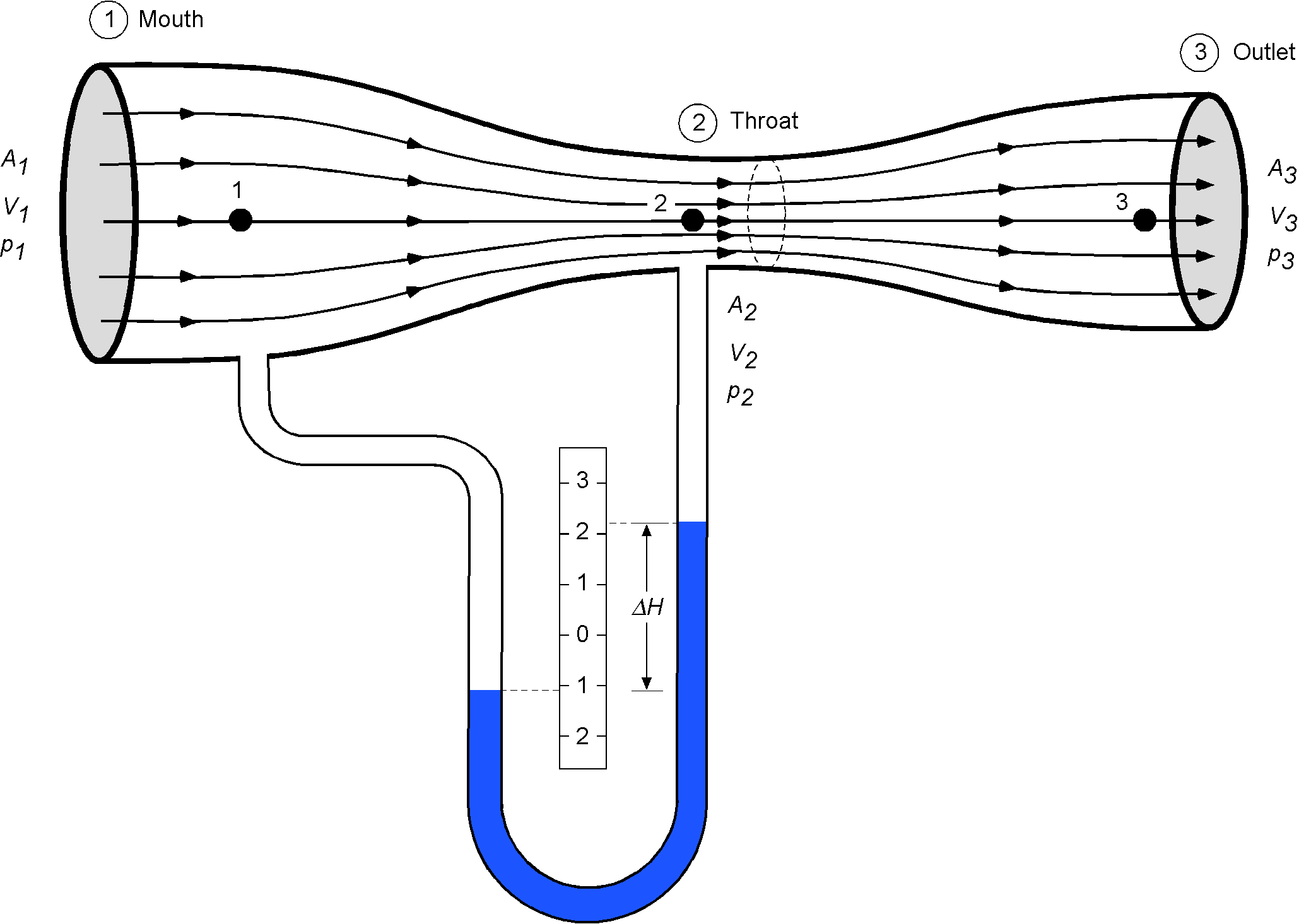
The advantages of a pressure drop in the throat of a Venturi are used in many practical engineering applications.

The intake to a Venturi is referred to as the mouth, and the narrowest part is called the throat. According to Bernoulli’s principle, a pressure drop occurs at the throat of a Venturi tube, where the flow accelerates. This behavior can be advantageous in several practical applications, such as flow meters, carburetors, and wind tunnels.

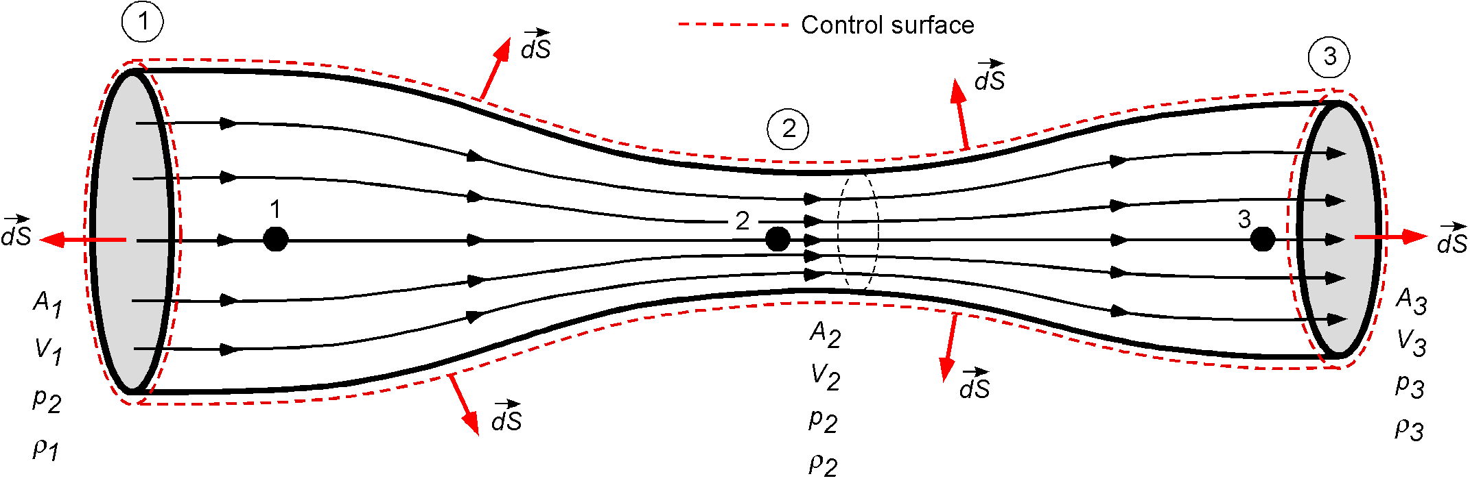
The first step in analyzing flow through a Venturi is to draw a control surface around the Venturi, with $\vec{n} \, dS = d\vec{S}$ pointing outward from the control volume by convention, as shown in Figure 2. Let the inlet conditions be at section 1, the throat at section 2, and the outlet at section 3. The cross-sectional areas in each case are assumed to be known, for example, through measurement. The flow can be considered steady and radially axisymmetric, i.e., an appropriate one-dimensional flow assumption.

Flow model for the flow through a Venturi.

The steady form of the continuity equation in integral form is

(1) $\begin{equation*} \oiint_S \varrho \, \vec{V} \bigcdot d\vec{S} = 0 \end{equation*}$

In words: “What mass flow comes into the control volume per unit of time then leaves the control volume in the same time, i.e., no fluid mass accumulates inside the control volume.”

There is no flow over the venturi’s walls, so the mass flow of fluid entering the venturi’s mouth per unit time also leaves at its exit. A one-dimensional flow assumption can significantly simplify the problem when cross-sectional area variation is relatively moderate. However, further consideration is needed of why a flow through a rapidly converging or expanding Venturi (or duct) may not be readily justifiable as a one-dimensional problem.

The flow enters the mouth of the Venturi of area $A_1$ with an average velocity ${V_1}$ , has a velocity ${V_2}$ at the throat of area ${A_2}$ , and a velocity $V_3$ at the exit of area ${A_3}$ . The fluid mass flow coming in is

(2) $\begin{equation*} \iint_{\rm intake} \varrho \, \vec{V} \bigcdot d\vec{S} = -\varrho_1 A_1 V_1 \end{equation*}$

The minus sign appears because the flow is opposite to the direction of $d\vec{S}$ at the entrance face. At the exit face, then

(3) $\begin{equation*} \iint_{\rm exit} \varrho \, \vec{V} \bigcdot d\vec{S} = \varrho_3 A_3 V_3 \end{equation*}$

Therefore, by using the continuity equation, then

(4) $\begin{equation*} \oiint_S \varrho \, \vec{V} \bigcdot d\vec{S} = \iint_{\rm intake} \varrho \, \vec{V} \bigcdot d\vec{S} + \iint_{\rm exit} \varrho \, \vec{V} \bigcdot d\vec{S} = 0 \end{equation*}$

which, for a one-dimensional flow, becomes

(5) $\begin{equation*} -\varrho_1 V_1 A_1 + \varrho_3 V_3 A_3 = 0 \end{equation*}$

If the flow is incompressible, $\varrho_1 = \varrho_2 = \varrho_3 = \varrho$ . Under these circumstances, the continuity equation can now be written as

(6) $\begin{equation*} -\varrho V_1 A_1 + \varrho V_3 A_3 = 0 \end{equation*}$

or

(7) $\begin{equation*} \varrho V_1 A_1 = \varrho V_3 A_3 = \overbigdot{m} \end{equation*}$

Also, it will be apparent that

(8) $\begin{equation*} \varrho V_1 A_1 = \varrho V_2 A_2 = \overbigdot{m} = \varrho \, Q \end{equation*}$

Canceling through the density gives

(9) $\begin{equation*} V_1 A_1 = V_2 A_2 = V_3 A_3 = Q \end{equation*}$

This equation states that the volume flow rate $Q$ through the Venturi is constant.

It can also be seen from the latter equation that, as the throat area decreases, the flow velocity must increase there to satisfy continuity, i.e., the mass and volume flow rates are constant at any cross-section. Conversely, if the throat area increases, the flow velocity must decrease. Moreover, from the previous discussion of Bernoulli’s equation, remember that when the velocity increases, the pressure decreases; conversely, when the velocity decreases, the pressure increases, i.e.,

(10) $\begin{equation*} p + \frac{1}{2} \varrho \, V^2 = \mbox{\small constant} \end{equation*}$

or

(11) $\begin{equation*} p_1 + \frac{1}{2} \varrho V_1^2 = p_2 + \frac{1}{2} \varrho V_2^2 \end{equation*}$

(12) $\begin{equation*} p_1 - p_2 = \frac{1}{2} \varrho \left( V_2^2 - V_1^2 \right) \end{equation*}$

The pressure difference $p_1 - p_2$ can be measured across the mouth and throat of the venturi, which can be accomplished by drilling two small holes^[2] (i.e., pressure taps) perpendicular to the Venturi walls at locations 1 and 2. The pressures are then measured by connecting tubes from these holes to a differential pressure gauge or the two sides (legs) of a U-tube manometer; see here for a simple experimental demonstration of this process. This pressure difference can then be related to the unknown velocity (or flow rate) through calculation or direct calibration using measurements.

From the continuity equation, then

(13) $\begin{equation*} V_{2} = V_{1}\left(\frac{A_1}{A_2}\right) \end{equation*}$

and from Bernoulli’s equation

(14) $\begin{equation*} p_{1} + \frac{1}{2}\varrho {V_{1}}^{2} = p_{2} + \frac{1}{2}\varrho {V_{2}}^{2} \end{equation*}$

Substituting gives

(15) $\begin{eqnarray*} p_{1} + \frac{1}{2} \varrho V_{1}^{2} & = & p_{2} + \frac{1}{2}\varrho V_{1}^{2} \left( \frac{A_1}{A_2} \right)^2 \\ p_{1} - p_{2} & = & \frac{1}{2} \varrho V_{1}^{2} \bigg( \left( \frac{A_1}{A_{2}} \right)^{2} - 1 \bigg) \end{eqnarray*}$

and so

(16) $\begin{equation*} Q = A_1 \sqrt{ \frac{2( p_{1} - p_{2})}{\varrho \bigg( \left( \displaystyle{\frac{A_{1}}{A_{2}} } \right)^{2} - 1 \bigg) } } \end{equation*}$

Therefore, given the pressure difference $p_{1} - p_{2}$ and the Venturi geometry (the area ratio), the flow rate $Q$ can be determined. Finally, notice that the change in pressure can be related to a change in the hydrostatic head of the fluid $\Delta h$ , using

(17) $\begin{equation*} p_{1} - p_{2} = \varrho_l \, g \, \Delta h \end{equation*}$

where $\varrho_l$ is the density of the liquid in the U-tube manometer.

Applications of a Venturi

A Venturi has many applications in practical engineering. Its primary characteristic is that the flow velocity is higher in the venturi’s throat. Consequently, the pressure at the throat is lower than the atmospheric pressure, and this pressure difference is helpful for various purposes.

Flowmeter (Venturimeter)

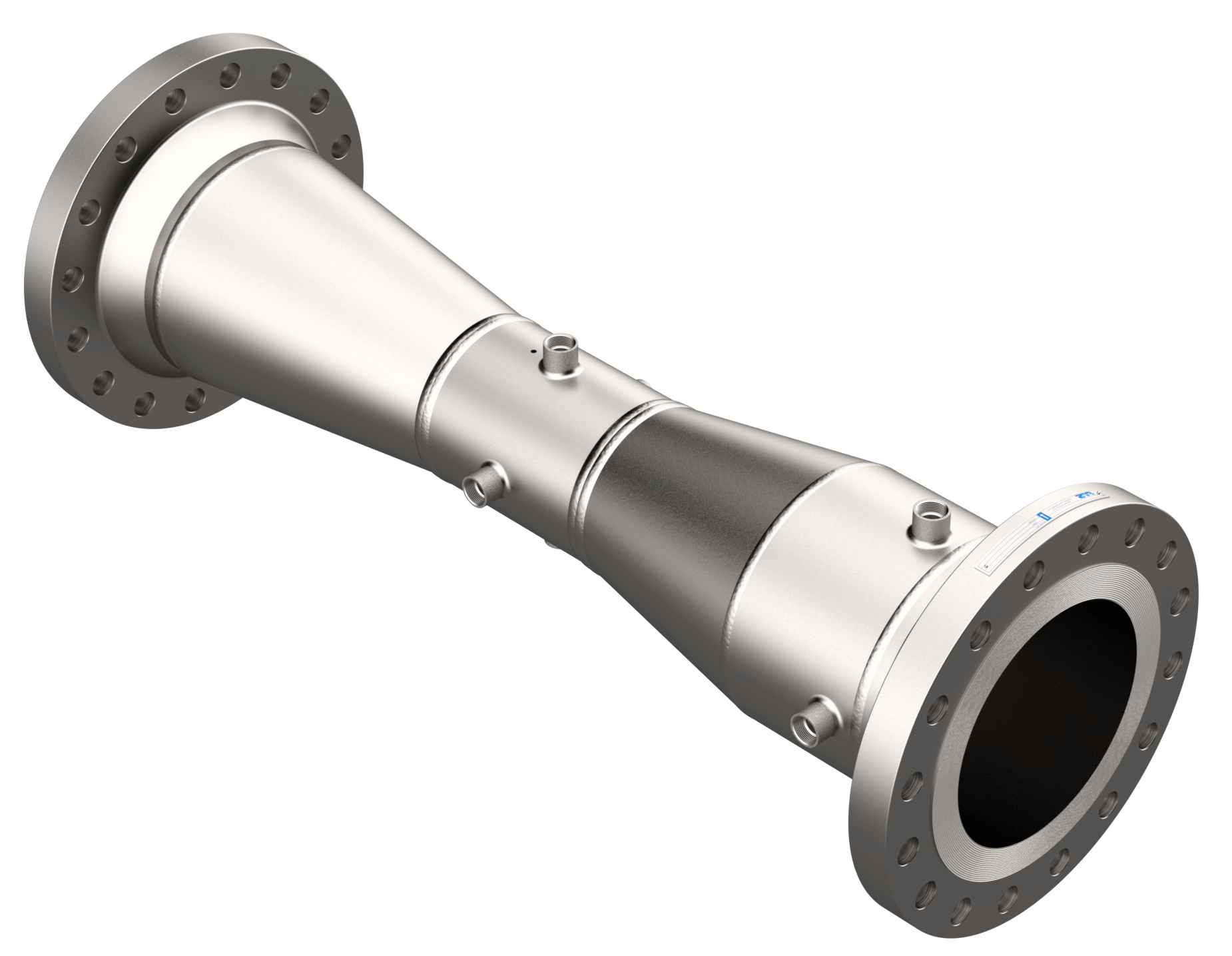
As the previous analysis suggests, a Venturi forms the basis for a device used to measure volume (or mass) flow rates. Such flowmeters, or Venturimeters as they are often called, are commercially available in various sizes and capacities. They are widely used in the water, chemical, pharmaceutical, and oil and gas industries to measure fluid flow rates along ducts and pipes, as shown in Figure 3. While venturimeters operate fundamentally on Bernoulli’s principle, which states that pressure decreases in the throat of the Venturi, they are usually factory-calibrated to account for losses, allowing volumetric flow rates to be more accurately related to the measured pressure drop across the throat. Four pressure taps are typically located at each section and are pneumatically averaged to provide a more consistent and accurate measurement of the static pressure drop between the entrance and the throat.

A classic Venturi meter measures the mass flow rate or volumetric flow rate of a fluid through a pipe.

The volumetric flow rate can be obtained from the ideal fluid assumption derived previously, with a correction factor to account for any viscous losses, i.e.,

(18) $\begin{equation*} Q = K_{\rm cal} \, A_1 \sqrt{ \frac{2( p_{1} - p_{2})}{\varrho \bigg( \left( \displaystyle{\frac{A_{1}}{A_{2}} } \right)^{2} - 1 \bigg) } } \end{equation*}$

where $K_{\rm cal}$ is a calibration factor. The value of $K_{\rm cal}$ is typically close to 1, but it depends on the specific Venturi.

Suction Source for Flight Instruments

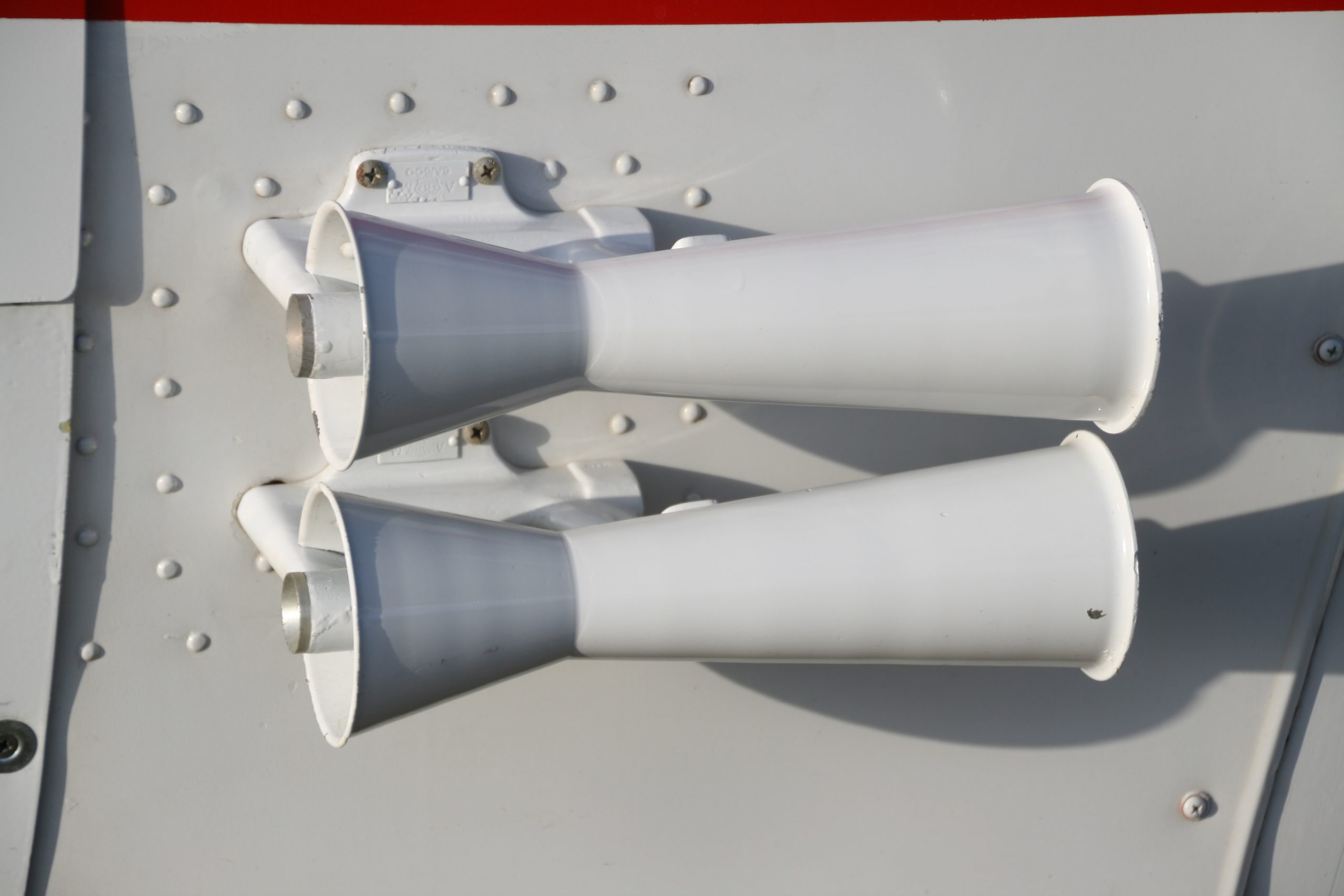
In early aircraft, a Venturi (or sometimes a pair of Venturi tubes) was mounted on the side of an aircraft’s fuselage, as shown in the photograph in Figure 4. The Venturi provided low suction pressure for air-driven gyroscopic instruments, such as the artificial horizon and directional gyro. Modern light aircraft, however, are fitted with mechanical, engine-driven vacuum pumps to provide the required suction pressure; therefore, venturis are no longer required.

A pair of Venturi tubes mounted on the side of an early aircraft provided low (suction) pressure to drive gyroscopic flight instruments.

From the continuity equation, the velocity at the throat, $V_t$ , for a given airspeed, ${V_{\infty}}$ , is

(19) $\begin{equation*} V_{t} = V_{\infty}\left(\frac{A_i}{A_t}\right) \end{equation*}$

where $A_i$ is the inlet area, and $A_t$ is the area of the throat. From the Bernoulli equation, then

(20) $\begin{equation*} p_{\infty} + \frac{1}{2}\varrho {V_{\infty}}^{2} = p_{t} + \frac{1}{2}\varrho {V_{t}}^{2} = p_{t} + \frac{1}{2}\varrho V_{\infty}^2\left(\frac{A_1}{A_2}\right)^2 \end{equation*}$

Therefore, the suction pressure available at the throat relative to static pressure is

(21) $\begin{equation*} p_{t} - p_{\infty} = \frac{1}{2}\varrho {V_{\infty}}^{2} \left( 1 - \left(\frac{A_1}{A_2}\right)^2 \right) \end{equation*}$

which shows that it decreases with the square of the airspeed at a given density altitude.

Carburetor

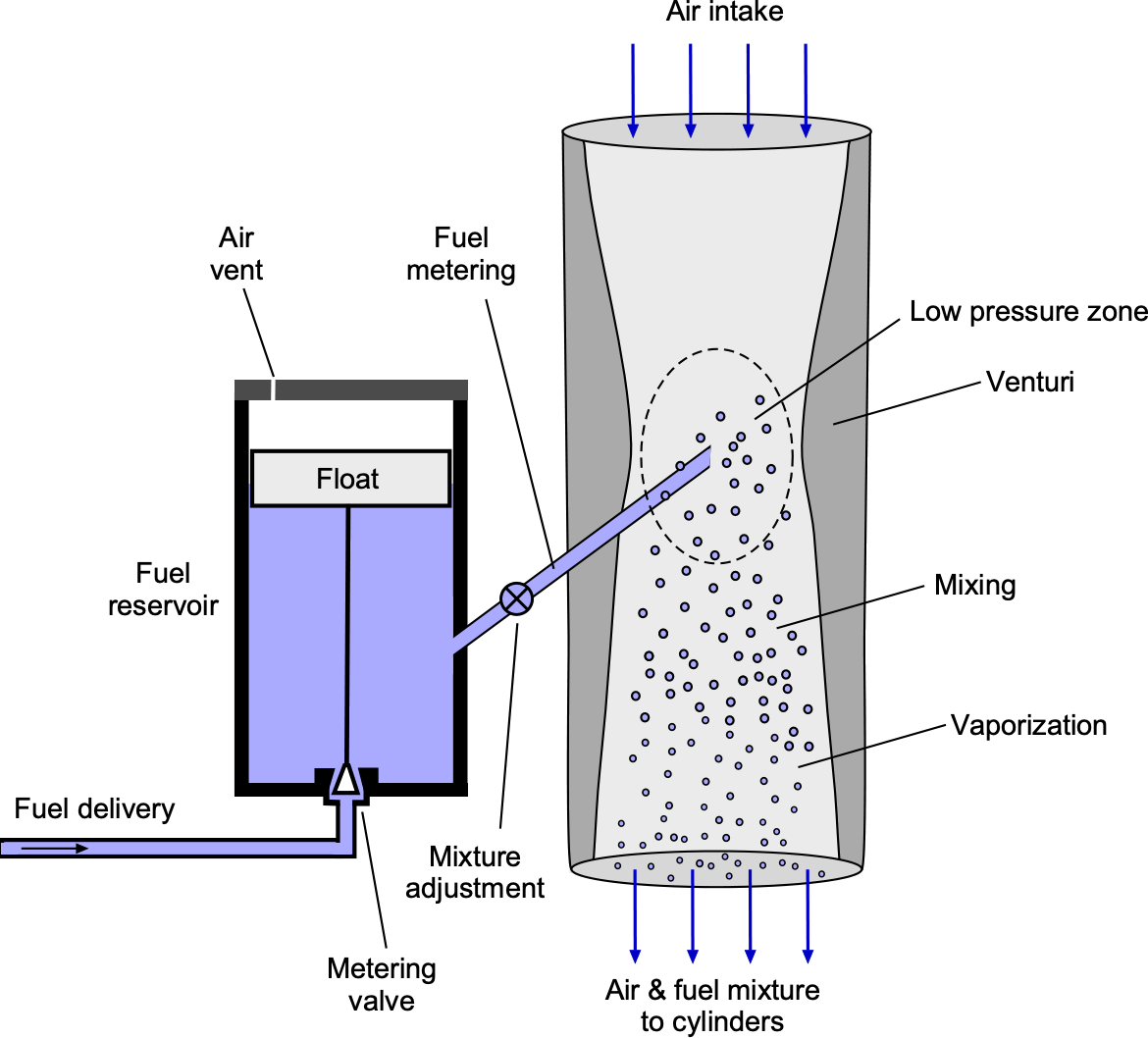
A carburetor provides an air-fuel mixture to a piston (reciprocating) engine. A carburetor has a Venturi that mixes incoming air with fuel, as shown in the schematics of Figure 5. Fuel from the tank is routed to a fuel reservoir, where a float maintains the fuel level. The fuel delivery line opens into the Venturi in the carburetor’s throat, where the fuel is first atomized. The lower pressure in this region helps draw fuel into the airstream, mix it with the air, and vaporize it downstream of the throat before the resulting fuel-air mixture enters the cylinders for combustion. Metering the fuel requires precise adjustment to ensure that the correct air-fuel mixture is delivered to each cylinder, thereby maximizing engine power and minimizing hydrocarbon emissions.

Flow Speed in a Wind Tunnel

A low-speed wind tunnel is a large Venturi in which the airflow is driven by a fan connected to a motor drive. The wind tunnel fan is a large propeller that efficiently moves air through the test section, as shown in Figure 6. This is an open-return or Eiffel-type wind tunnel, while the other type is a closed-return or loop type.

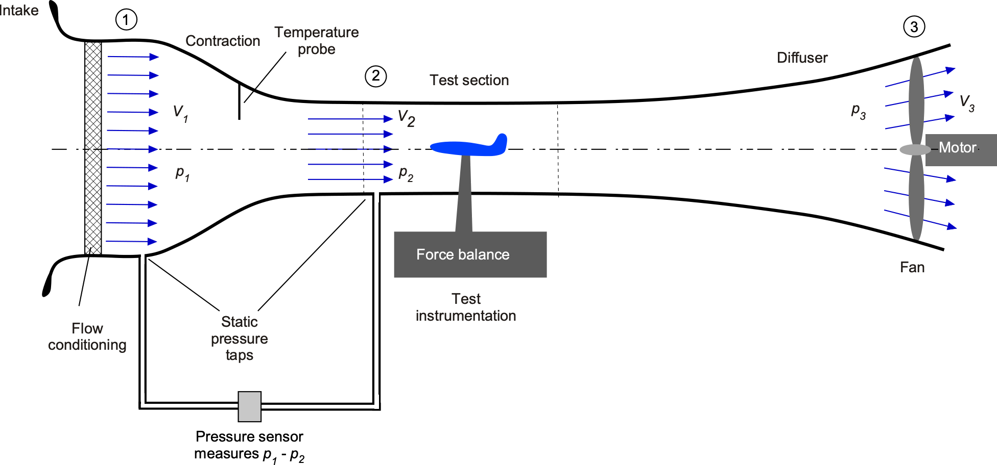
The static pressure drop between the wind tunnel intake and test sections can be measured to determine the flow speed in the test section.

The airflow enters the mouth of area $A_1$ at a flow velocity ${V_1}$ with pressure $p_1$ . The wind tunnel then contracts to a smaller area, ${A_2}$ , at the test section, where the velocity has increased to ${V_2}$ . The velocity in the test section must increase to satisfy the continuity condition. The model (e.g., a wing or a complete aircraft model) is placed in the test section, where its aerodynamic characteristics are measured and recorded. The flow then passes downstream into a diverging duct (diffuser), where, just before the fan, the area is ${A_3}$ , the velocity is $V_3$ , and the pressure is $p_3$ .

From the continuity equation, the air velocity in the test section is

(22) $\begin{equation*} V_2 = \left( \frac{A_1}{A_2} \right) V_1 \end{equation*}$

In turn, the velocity at the exit of the diffuser before the fan is

(23) $\begin{equation*} V_3 = \left( \frac{A_2}{A_3} \right) V_2 \end{equation*}$

The pressure at various locations in the wind tunnel is related to the velocity by Bernoulli’s equation

(24) $\begin{equation*} p_1 + \frac{1}{2} \varrho V_1^2 = p_2 + \frac{1}{2} \varrho V_2^2 = p_3 + \frac{1}{2} \varrho V_3^2 \end{equation*}$

The velocity in the working or test section (the most important quantity) can be related to the pressure drop between sections 1 and 2, i.e., between the mouth of the contraction section and the test section. From the Bernoulli equation, then

(25) $\begin{equation*} V_2^2 = \frac{2}{\varrho} \left( p_2 - p_1 \right) + V_1^2 \end{equation*}$

This means that

(26) $\begin{equation*} V_2^2 = \frac{2}{\varrho} \left( p_1 - p_2 \right) + \left( \frac{A_2}{A_1} \right)^2 V_2^2 \end{equation*}$

Solving for ${V_2}$ (the flow velocity in the test section) gives

(27) $\begin{equation*} V_{2} = \sqrt{ \frac{2\left(p_{1} - p_{2}\right)}{\varrho \bigg( 1 - \left( \displaystyle {\frac{A_{2}}{A_{1}} }\right)^{2} \bigg) } } \end{equation*}$

The area ratio $A_2/A_1$ is fixed for a given wind tunnel. Please remember that the density is a constant for an incompressible flow. Its value can be obtained from measurements of static pressure and temperature, along with the equation of state.

Therefore, the above equation can be used to determine the velocity in the test section by measuring the pressure drop from the intake to the contraction, and from the contraction to the test section. This latter technique is used in most low-speed wind tunnels to measure flow speed in the test section: the pressure drop between a point on the contraction and the test section is measured. This pressure drop is then related to the flow velocity in the test section via Bernoulli’s equation and subsequently verified by calibration. In the calibration, a Pitot probe (see discussion below) is placed in the test section, and the pressure drop is measured for a range of flow speeds; any discrepancy leads to a calibration factor, $K_{\rm cal}$ , that can be used to determine the flow speed more accurately, i.e., using

(28) $\begin{equation*} V_{2} = \sqrt{ \frac{2 \, K_{\rm cal} \left(p_{1} - p_{2}\right)}{\varrho \bigg( 1 - \left( \displaystyle {\frac{A_{2}}{A_{1}} }\right)^{2} \bigg) } } \end{equation*}$

In practice, the calibration factor for a low-speed wind tunnel is close to 1.

Cavitating Venturi

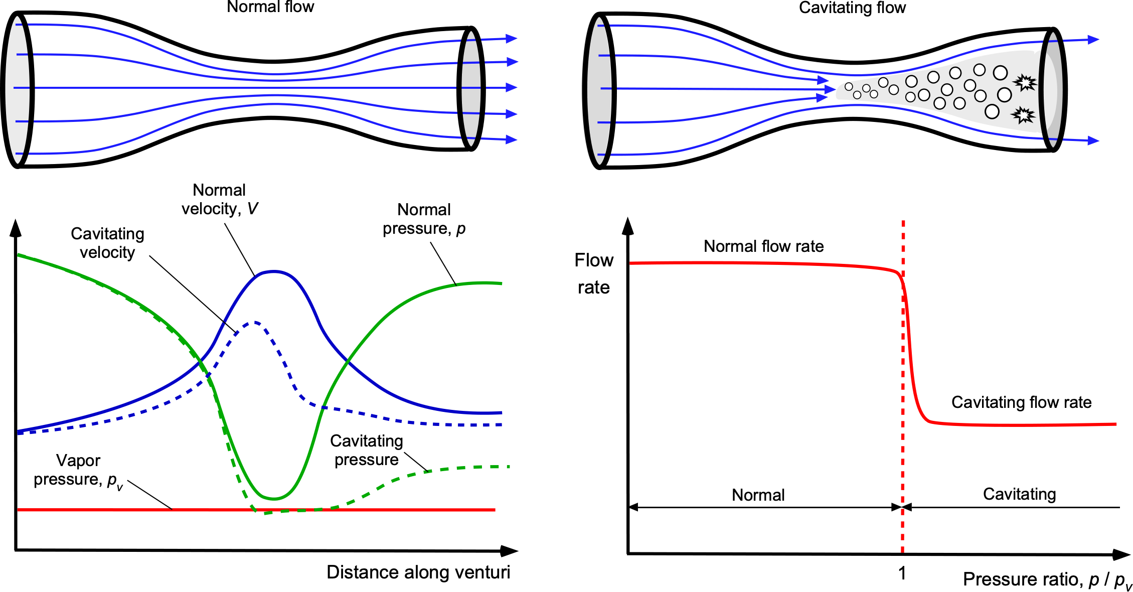
Cavitating venturis can be used to control or limit the flow rate of a liquid through a pipe. The throat of a cavitating Venturi is sized such that for a given differential pressure drop between the inlet and the throat, the pressure at the throat is reduced to its vapor pressure point, $p_v$ , as illustrated in Figure 7. The resulting vapor and bubbles, known as cavitation, are analogous to boiling without the addition of heat. This phenomenon will limit the mass flow rate through the Venturi, preventing any further increase in mass flow rate at a given upstream inlet pressure. As the bubbles travel downstream into the throat, they eventually burst, and the static pressure returns to its pre-cavitation value. The mass flow rate through the pipe is independent of the downstream pressure; therefore, the mass flow can be controlled by changing the inlet pressure, and hence the amount of cavitation in the throat. Cavitating venturimeters are often used as propellant mass flow limiters in rocket engines.

The cavitation number is usually expressed as

(29) $\begin{equation*} C_{\rm cav} = \dfrac{p - p_v}{\frac{1}{2} \varrho V_t^2} \end{equation*}$

where $V_t$ is the flow velocity at the throat. This is a form of pressure coefficient, so cavitation will first occur at $C_{\rm cav} = 1$ . The volumetric flow rate through a Venturi is given by

(30) $\begin{equation*} Q = A_1 \sqrt{ \frac{2( p_{e} - p_{t})}{\varrho \bigg( \left( \displaystyle{\frac{A_{e}}{A_{t}} } \right)^{2} - 1 \bigg) } } \end{equation*}$

where $p_e$ is the entrance pressure to the venturi, and $p_t$ is the pressure in the throat. The entrance area is $A_t$ , and the throat area is $A_t$ , both of which can be measured. If the pressure in the throat equals the vapor pressure, i.e., $p_t = p_v$ and $C_{\rm cav} = 1$ , then the flow rate will become cavitation-limited to a maximum value of

(31) $\begin{equation*} Q_{\rm max} = A_e \sqrt{ \frac{2( p_{e} - p_{v})}{\varrho \bigg( \left( \displaystyle{\frac{A_{e}}{A_{t}} } \right)^{2} - 1 \bigg) } } \end{equation*}$

Once this point is reached, further increases in upstream pressure will be ineffective in increasing the flow rate. Vapor pressures, $p_v$ , for various liquids at different temperatures are available in online resources and in the table below. Knowing the vapor pressure also allows the Venturi to be designed to limit volumetric or mass flow rate. For example, for given values of $Q_{\rm max}$ , $p_e$ , and $A_1$ , the throat area $A_t$ can be determined to limit the flow rate from the onset of cavitation.

**Vapor pressures of different liquids at a temperature of 25°C (77°F)**
Liquid	Vapor pressure (Pa)	Vapor pressure (lb/ft²)
Water	3,166.6	0.0666
JET-A	~ 2,000	~ 0.04206
100LL gasoline	~ 40,000	~ 0.8413
Ethanol	5,853.7	0.1227
Acetone	24,266.4	0.5085
Diethyl ether	53,465.3	1.1195
Methanol	16,931.5	0.356316
Hexane	19,995	0.4201
Chloroform	26,384.9	0.5543
Carbon tetrachloride	12,125.7	0.2555
Benzine	12,661.2	0.2673

Siphon (Syphon)

A siphon, also spelled syphon, is a device used to transfer liquids from one level to another. It consists of a tube or hose bent into a U-shape, with one end placed in a liquid, such as water, and the other end set at a lower level, as shown in Figure 8. This arrangement allows water to flow from the tank to a lower level, relying on gravity and hydrostatic pressure. To initiate flow, the siphon tube must be filled with water. This can be done by evacuating air from the tube or by filling it with water and submerging one end in the tank. Once the flow starts, it will continue until the tank is emptied.

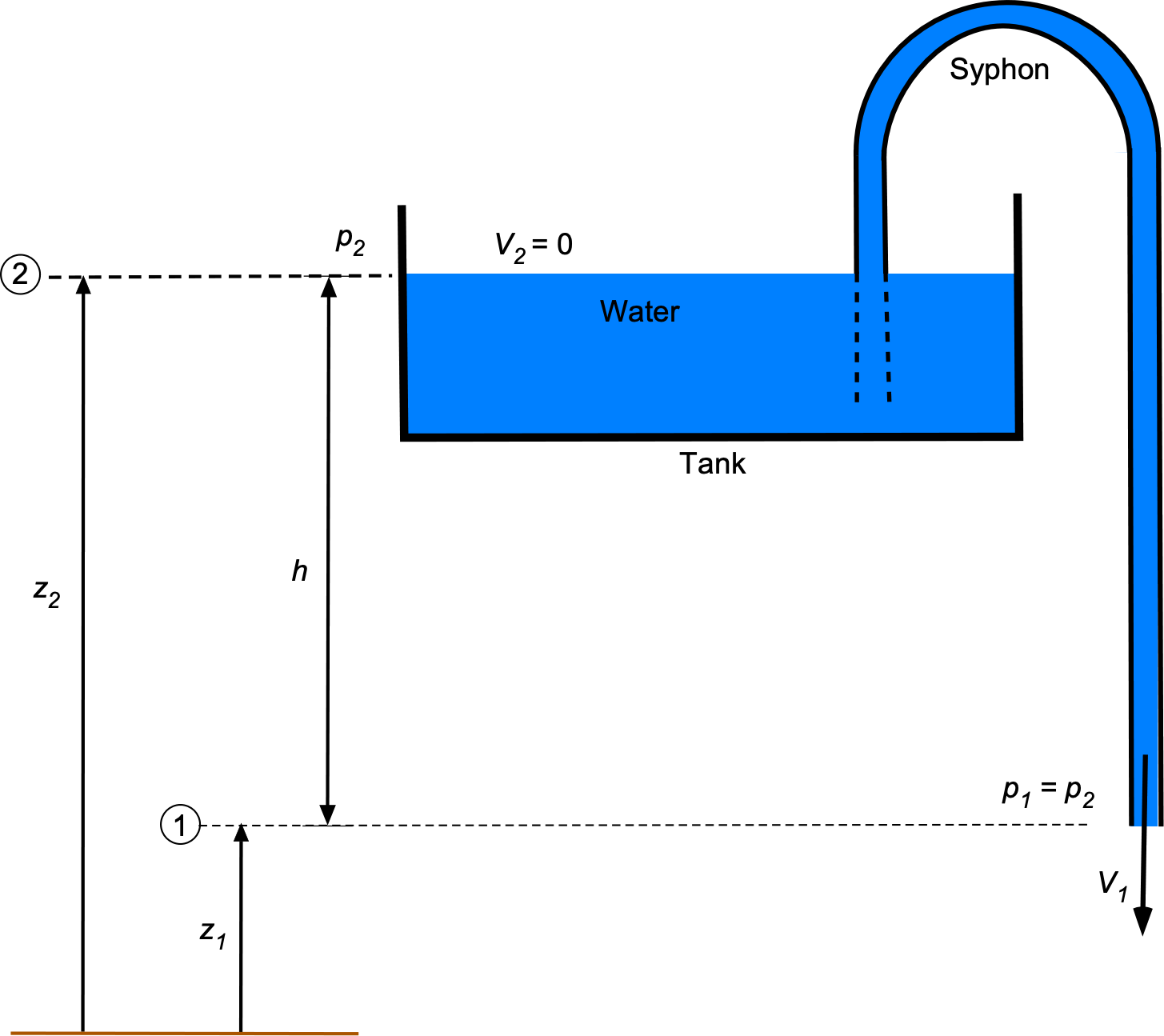
The principle of a siphon is used to transfer a liquid from a container placed at a higher level to a lower level.

It is often claimed that a siphon works on the principle of air pressure, but this is incorrect. To see why, the Bernoulli equation applied in the fluid between the tank and the outlet from the siphon gives

(32) $\begin{equation*} p_1 + \frac{1}{2} \varrho V_1^2 + \varrho \, g \, z_1 = p_2 + \frac{1}{2} \varrho V_2^2 + \varrho \, g \, z_2 \end{equation*}$

The change in air pressure between the levels at ${z_1}$ and ${z_2}$ is minimal, so it can be assumed that $p_1 = p_2$ . Also, if the fluid in the tank is assumed to be of much greater volume than the volume flow rate out of the siphon, then ${z_2}$ = constant. Therefore, under these quasi-steady assumptions, the Bernoulli equation becomes

(33) $\begin{equation*} p_1 + \frac{1}{2} \varrho V_1^2 + \varrho \, g \, z_1 = p_1 + 0 + \varrho \, g \, z_2 \end{equation*}$

or

(34) $\begin{equation*} \frac{1}{2} V_1^2 + g \, z_1 = g \, z_2 \end{equation*}$

Rearranging gives the outlet flow velocity as

(35) $\begin{equation*} V_1 = \sqrt{ 2 \, g \left( z_2 - z_1 \right)} = \sqrt{ 2 \, g \, h} \end{equation*}$

which is called Torricelli’s law.^[3] Notice that the flow velocity depends on the difference in the height of the water, ${h}$ , and acceleration under gravity, so the higher the height difference, the faster the water will flow. There is no significant change in atmospheric pressure between the two levels. Therefore, the siphon effect is produced by the hydrostatic pressure difference within the liquid, not the (slight) difference in atmospheric air pressure.

However, considering viscous effects (and hence losses) will change this result, as there will be a slight pressure drop along the length of the siphon tube. Calculating such internal pressure losses and flow velocity requires a viscous flow theory, which will be considered in a later chapter of this ebook.

Total, Static, & Dynamic Pressures

It must now be explained more precisely what the total and static pressures of a fluid mean. Consider a flow moving with velocity $V$ at a pressure $p_{s}$ . If moving with the velocity of the airflow, then the pressure that will be felt is $p_{s}$ . This latter pressure is called static pressure and measures the effects of the random motion of fluid molecules. Now, if the boundary or “wall” of a flow is considered (e.g., the wall of a duct, pipe, or wind tunnel), and a small hole in the wall is drilled in a direction perpendicular to the flow, then the pressure that is measured there would be the static pressure $p_{s}$ .

Suppose a U-tube manometer is connected, as shown in Figure 9, and the open end outside the flow (i.e., the reference end) of the manometer is at a lower static pressure than in the flow. In that case, a height difference $h_s$ will be observed on the manometer. The pressure is the static pressure relative to the ambient reference pressure, called the gauge pressure. If the static pressures inside and outside are equal, then $h_s = 0$ .

Concepts of the measurement of static pressure, total pressure, and dynamic pressure.

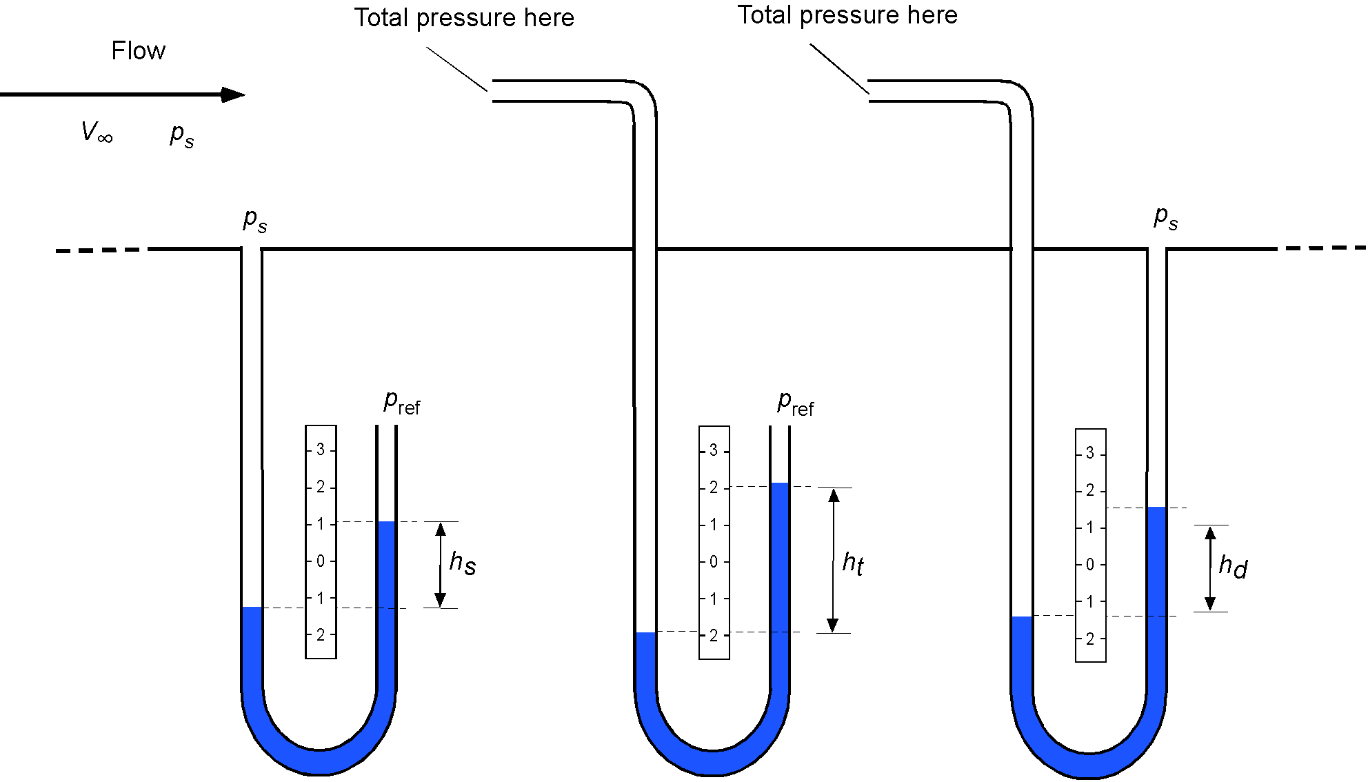
Now consider a Pitot tube (after the hydraulic engineer, Henri Pitot) inserted into the flow, which is an open tube with its end facing into the flow. The fluid cannot flow through the tube, causing it to stagnate; i.e., the flow velocity goes to zero at the tube entrance because there is no place for the fluid to flow. Hence, the streamline that infringes directly on the mouth of the Pitot tube will have zero velocity; this location is called a stagnation point. In this case, the pressure that is measured is called the total pressure, $p_T$ , which is the sum of the dynamic pressure and the static pressure, i.e.,

(36) $\begin{equation*} p_T = p_s + \frac{1}{2} \varrho \, V^2 \end{equation*}$

where $\varrho$ is the density of the flowing fluid, with an equivalent height of the hydrostatic head on the manometer of $h_t$ .

Finally, consider the case in which the reference pressure is the static pressure in the flow. In this case, the pressure would be the dynamic pressure of the flow, i.e., the difference between the total pressure and the static pressure

(37) $\begin{equation*} p_s + \frac{1}{2} \varrho \, V^2 - p_s = \frac{1}{2} \varrho \, V^2 \end{equation*}$

with an equivalent hydrostatic head of $h_d$ on the manometer.

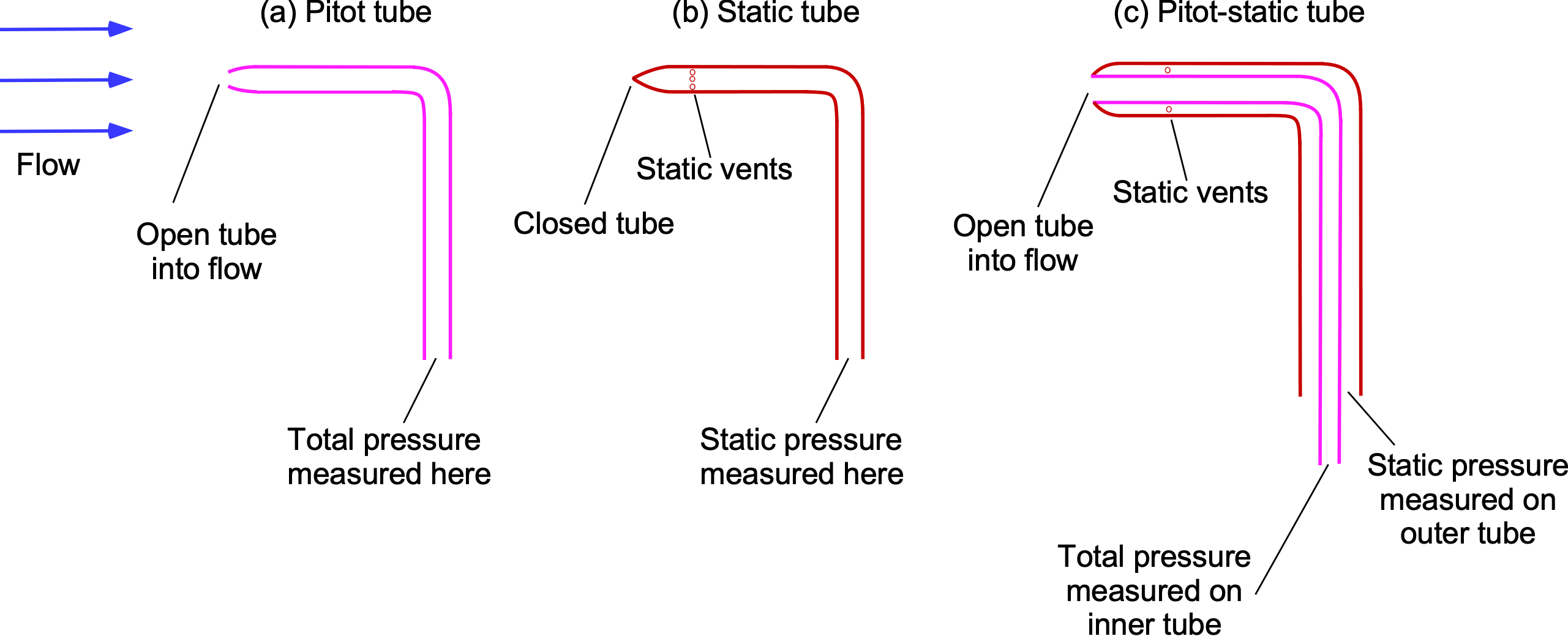
Pitot Tube & Pitot-Static Tube

Pitot probes (or Pitot tubes), static probes, and Pitot-static probes are often used to measure flow velocities. In each case, the principle is the same: pressure measurements can be used with the Bernoulli equation to calculate the flow velocity. The proviso is that the flow density at the probe insertion point is known. These three types of pressure probes are shown in Figure 10.

When a Pitot tube and static tube are combined into a single unit, it is called a Pitot-static tube (or probe). A “static tube” can be used to measure static pressure in a flow.

For the analysis of a Pitot tube, consider point 1 upstream of the Pitot tube and point 2 at the entrance to the tube, as shown in Figure 11. From Bernoulli’s equation it is known that $p+1/2\varrho V^{2} =$ constant along any given streamline, so that

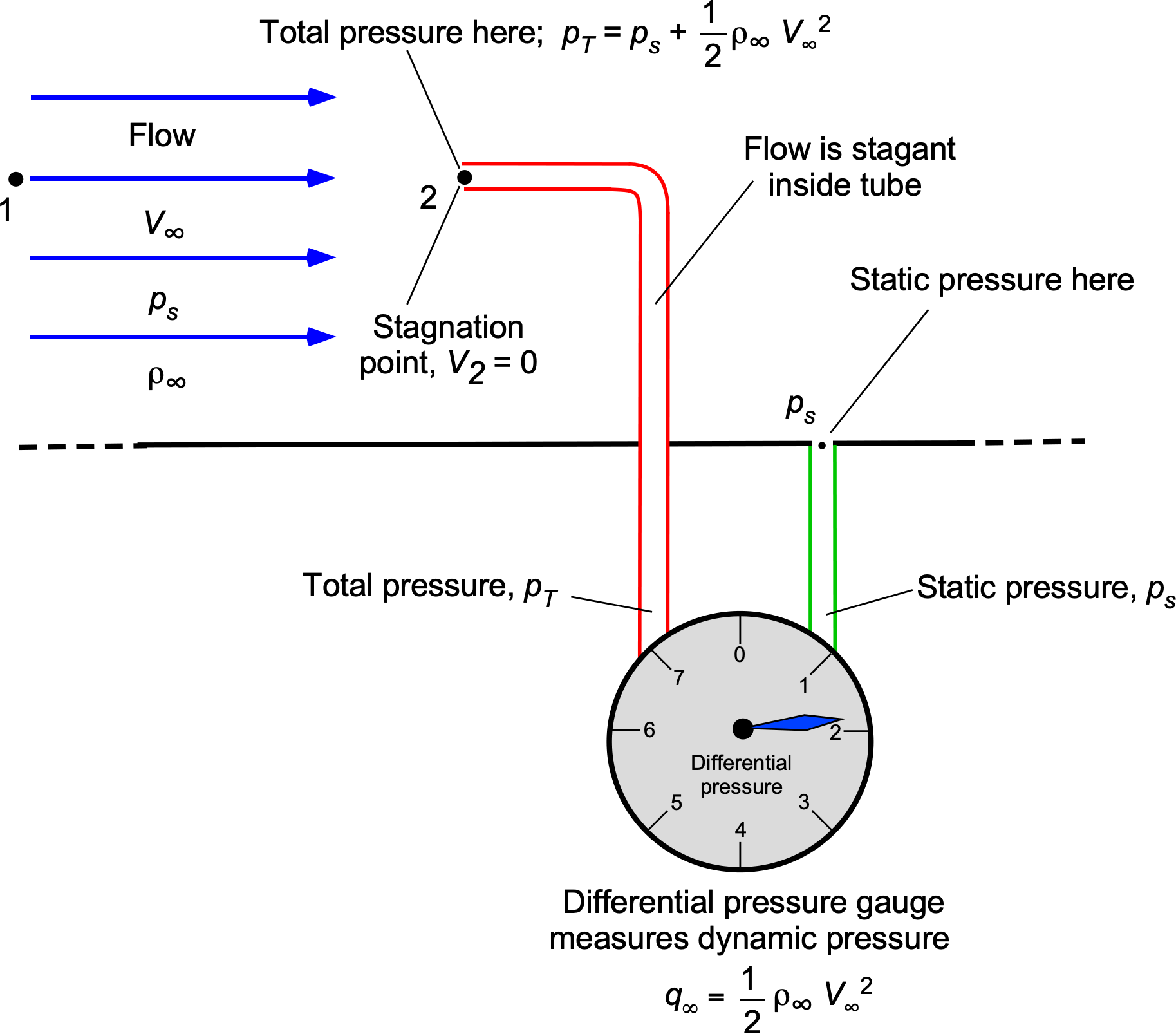
(38) $\begin{equation*} p_{1} + \frac{1}{2} \varrho_{\infty} V_{1}^{2} = p_{2} + \frac{1}{2} \varrho V_{2}^{2} = p_T = p_{\infty} + \frac{1}{2} \varrho_{\infty} V_{\infty}^{2} \end{equation*}$

The difference in pressure between total pressure and static pressure can be measured on a suitably calibrated pressure gauge.

But at point 2 at the entrance to the Pitot tube, the fluid is brought to rest so $V_{2} = 0$ (i.e., it is a stagnation point), and so

(39) $\begin{equation*} p_1 + \frac{1}{2} \varrho_{\infty} V_{1}^2 = p_{2} = p_T =\mbox{\small Total pressure at point 2} \end{equation*}$

The static pressure $p_1 = p_{s} = p_{\infty}$ must be measured to obtain the flow velocity from this latter expression. As in the Venturi problem, this static pressure can be measured using a separate static vent or static ports on the outer side of a concentric Pitot-static tube. Solving for $V_{1}$ gives

(40) $\begin{equation*} V_{1} = \sqrt{\frac{ 2\left(p_{T} - p_{s}\right)}{\varrho_{\infty}}} = \sqrt{\frac{ 2\left(p_{T} - p_{\infty}\right)}{\varrho_{\infty}}} \end{equation*}$

Therefore, the upstream flow velocity can be determined from the difference between the flow’s total and static pressures. Again, this pressure difference can be measured using a differential gauge, manometer, or pressure transducer.

The preceding principles are used in airspeed measurement with an Air Speed Indicator (ASI), which is part of the aircraft’s pneumatic system for not only airspeed but also altitude and rate of climb, as shown in Figure 12. An airspeed indicator is a suitably calibrated differential pressure gauge. The dynamic pressure source needed for an airspeed indicator is either a Pitot tube or a Pitot-static tube. Notice, in this case, the use of a Pitot probe to measure the total pressure and a separate static vent (usually placed somewhere on the side of the fuselage) to measure the reference pressure. A heater prevents the Pitot probe from malfunctioning in icing conditions by preventing ice accumulation on the exposed probe.

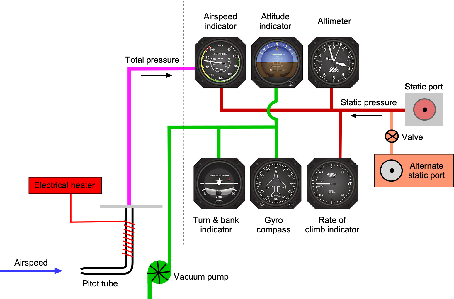
A Pitot-static system on an airplane provides the reference pressures needed for the airspeed indicator and other pneumatic instruments. Notice that, in this case, a Pitot probe is used to measure total pressure, and a separate static port is used to measure static pressure.

More often than not, airplanes use Pitot tubes (to measure total pressure $p_T$ ) with static taps (to measure $p_s$ ) located elsewhere on the airframe, as previously shown. In this case, then the airspeed ${V_{\infty}}$ will be

(41) $\begin{equation*} V_{\infty} = \sqrt{\frac{ 2\left(p_{T} - p_{s}\right)}{\varrho_{\infty}}} \end{equation*}$

In either case, the purpose is the same: to measure the aircraft’s airspeed. This information is then provided to the pilot on an airspeed indicator. Therefore, an airspeed indicator is a dynamic-pressure gauge calibrated in units of speed; typically, nautical miles per hour (kts) are used, but sometimes miles per hour (mph). An online simulator of the Pitot-static system helps users understand how it works and how it behaves under various failure scenarios.

Flow Speed in a Wind Tunnel (Take 2)

While it has been previously described that the flow speed in the test section of a wind tunnel can be obtained by measuring the static pressure drop between the inlet and the test section, an alternative is to use a Pitot probe, as shown in Figure 13. The Pitot probe measures the total pressure, $p_T$ , in the upstream section, or in any upstream section convenient for measurement. This approach tends to yield a more accurate measure of dynamic pressure because it is the difference between a higher and a lower pressure, rather than between two lower pressures of similar magnitude.

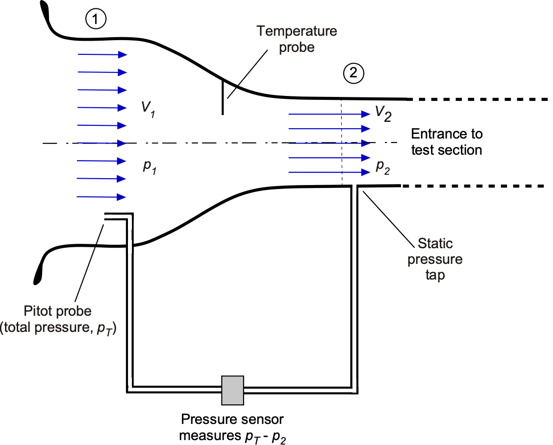
Another method of measuring the flow velocity in a wind tunnel is to use measurements of total pressure and static pressure.

From the Bernoulli equation, then

(42) $\begin{equation*} P_T = p_2 + \dfrac{1}{2} \varrho V_2^2 = p_{\infty} + \dfrac{1}{2} \varrho V_{\infty}^2 \end{equation*}$

so that

(43) $\begin{equation*} V_2 = V_{\infty} = \sqrt{ \frac{2 \left( p_T - p_{\infty} \right)}{\varrho_{\infty}} } \end{equation*}$

Again, the value of density, $\varrho_{\infty}$ , can be obtained from static pressure and temperature measurements in conjunction with the equation of state. The calibration would be verified by placing a Pitot probe in the test section to obtain any calibration factor, $K_{\rm cal}$ , i.e.,

(44) $\begin{equation*} V_{\infty} = K_{\rm cal} \sqrt{ \frac{2 \left( p_T - p_{\infty} \right)}{\varrho_{\infty}} } \end{equation*}$

where $K_{\rm cal}$ will be very close to unity.

Tesla Valve

Consider the branched circuit shown in Figure 14, which has a central main line and three loops. The question is: what happens to the flow as it moves through this unusual branched circuit? Two cases are to be examined. Case A depicts a flow entering from the right and exiting to the left. Case B is when the flow enters from the left and leaves to the right. The section title suggests that this situation involves valve-like action and that flow behavior differs depending on the direction. Recall that a valve is a device used to regulate or limit the flow of a fluid. In understanding the flow, one immediately considers applying the principle of continuity (mass or volume conservation) to the quantity of fluid entering and leaving.

Consider a single branch loop of this system, as shown in Figure 15. In Case A (right to left), very little fluid will pass around the branch loop compared to what goes through the main line. Even if some fluid does go through the branch, it simply rejoins the main flow downstream. By continuity considerations, the flow rate entering the branch loop equals the flow rate leaving, so the branch loop has no net effect on the main flow.

Flow model for one loop of a Tesla valve. With the flow from left to right, the branch loop will stagnate, effectively limiting the volumetric flow rate.

In Case B (left to right), the flow path is more interesting because some of the flow will split at the first Y-branch, go around the branch loop, and then rejoin the main line in the opposite direction at the second Y-branch, in effect forming a stagnation loop. The upshot is that the stagnation loop acts as a flow restrictor in the main line. In this case, continuity considerations suggest that the net forward flow rate in the main line will be progressively reduced as the fluid moves through the system from loop to loop.

The simple one-dimensional incompressible form of the continuity equation can be used to quantitatively explain the essential one-way flow behavior of a Tesla valve, without considering viscosity or pressure losses. Let the initial incoming volumetric flow rate be $Q$ , which is also the unimpeded flow rate in Case A. After point 1, a fixed volume fraction, $f$ , of the main flow will be diverted through the loop, and the remainder continues along the main line. The volumetric flow rate in the branch loop is

(45) $\begin{equation*} Q_{\mathrm{loop}} = f \, Q \end{equation*}$

and by continuity, the remainder of the flow continues along the main line, i.e., the volume flow rate there is

(46) $\begin{equation*} Q_{\mathrm{main}} = (1 - f) \, Q \end{equation*}$

The flow in the branch loop returns to meet the main flow in the opposite direction at the second Y-junction, whose outlet is directed upstream. Therefore, at least based on one-dimensional assumptions, the net volumetric flow after the stage is the difference between the volumetric flows in the main line and the opposing loop flow, i.e., the net flow rate at point 2 will be reduced to

(47) $\begin{equation*} Q_1 = (1 - f) \, Q - f \, Q = (1 - 2f) \, Q \end{equation*}$

In effect, the branch loop becomes a stagnation-flow loop, thereby limiting the net flow rate through the main line. Therefore, net continuity considerations dictate that the initial unimpeded flow rate $Q$ throughout the system is now reduced to $Q_1$ .

For $n$ identical loops in series, the same factor $(1-2f)$ is then applied at each stage, giving a net flow rate of

(48) $\begin{equation*} Q_n = (1 - 2 f)^{\,n} \, Q \end{equation*}$

where $Q$ is the initial or unimpeded flow rate. Therefore, after several stages, the net flow rate through the system is simply the initial flow rate multiplied by $(1-2f)^{n}$ . For example, if $f = \dfrac{1}{3}$ , after three stages the net flow rate will be $\left(\dfrac{1}{3}\right)^3 Q = \dfrac{1}{27} \, Q$ . Therefore, one can conclude that a Tesla valve is a one-way valve, allowing fluid to flow easily in one direction but not the other. This is a very clever device because it acts as a flow valve with no moving parts.

In practice, the performance of a Tesla valve is more complex than what has been described using this ideal model, a nice viscous flow simulation being shown here; yet the stagnation loops and the progressive reduction in the net flow as the fluid reaches each stage are obvious. The volume fraction $f$ depends on the relative hydraulic resistance of the main path and the loop, which varies with flow rate and, hence, the Reynolds number. Additional effects arise from turbulence, flow separation, and losses at junctions and bends. These effects make the one-way valve action more effective at higher flow rates, but also mean that the simple continuity model provides only a basic understanding of how it works rather than a quantitatively accurate prediction of its actual performance.

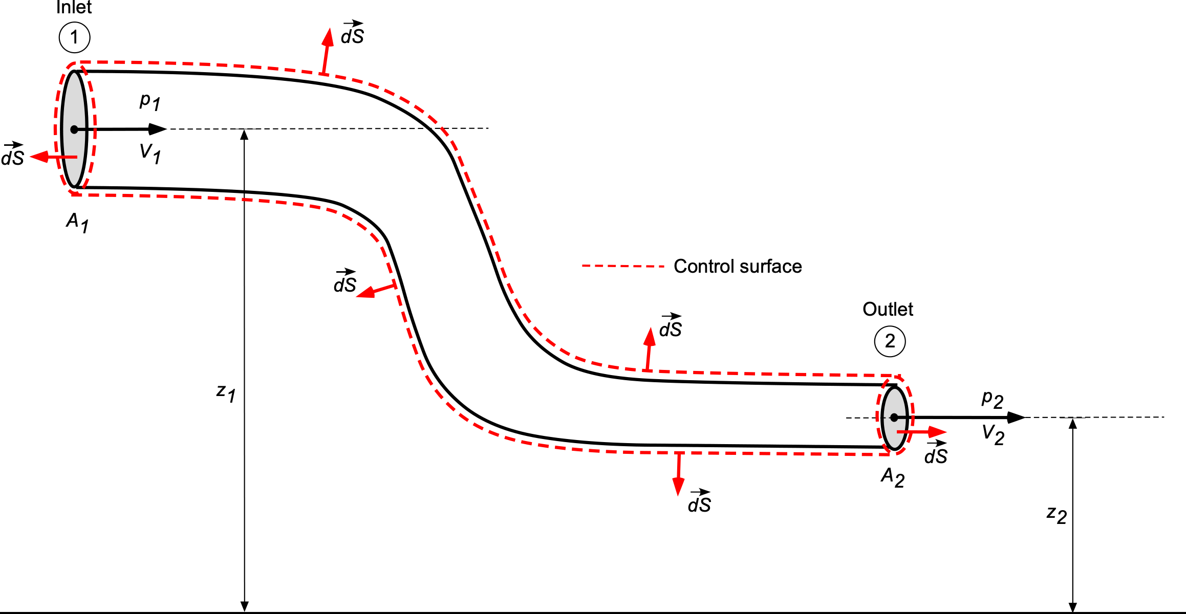
Force on a Pipe Bend

The determination of flow rates, flow velocities, pressures, and forces on fluids flowing through pipes and channels is a typical application of the conservation laws in integral form. Consider a flow through a pipe of circular cross-section that encounters a change in the area and height of the pipe as it passes through an elbow-type coupling, as shown in Figure 16. The pipe lies in a vertical plane, e.g., the ${x}$ – ${z}$ plane. Assume uniform flow properties across any cross-section and no losses, and that the fluid is water of density $\varrho_w$ .

Flow model for the flow through an elbow-type coupling.

The flow rate, $Q$ , or the mass flow rate $\overbigdot{m}$ , is usually given, as well as the input and output areas, so that conservation of mass gives

(49) $\begin{equation*} \overbigdot{m} = \varrho_w A_1 V_1 = \varrho_w A_2 V_2 \implies Q = A_1 V_1 = A_2 V_2 \end{equation*}$

Therefore, the flow velocities are given by

(50) $\begin{equation*} V_1 = \dfrac{Q}{A_1} = \dfrac{\overbigdot{m}}{\varrho_w \, A_1} \quad \text{and} \quad V_2 = \dfrac{Q}{A_2} = \dfrac{\overbigdot{m}}{\varrho_w \, A_2} \end{equation*}$

Using the Bernoulli equation gives

(51) $\begin{equation*} p_1 + \frac{1}{2} \, \varrho_w \, V_1^2 + \varrho_w \, g \, z_1 = p_2 + \frac{1}{2} \, \varrho_w \, V_2^2 + \varrho_w \, g \, z_2 \end{equation*}$

If, for example, $p_1$ is a known value, then rearranging to solve for $p_2$ gives

(52) $\begin{equation*} p_2 = p_1 + \frac{1}{2} \varrho_w \, \left( V_2^2 - V_1^2 \right) + \varrho_w \, g \left( z_2 - z_1 \right) \end{equation*}$

The force on the pipe can be obtained by summing the net pressure forces and the time rate of change of momentum. It will be apparent that the pressure force and momentum change only in the ${x}$ direction. The one-dimensional form of the momentum equation becomes

(53) $\begin{equation*} F_{x} + (p_1 \, A_1 - p_2 \, A_2) = \overbigdot{m} V_2 - \overbigdot{m} V_1 = \overbigdot{m} \left( V_2 - V_1 \right) = \varrho_w \, Q \left( V_2 - V_1 \right) \end{equation*}$

where $F_x$ is the force on the fluid, so that

(54) $\begin{equation*} F_x = \left( p_2 \, A_2 - p_1 \, A_1 \right) + \overbigdot{m} \left( V_2 - V_1 \right) = ( p_2 \, A_2 - p_1 \, A_1) + \varrho_w \, Q \, \left( V_2 - V_1 \right) \end{equation*}$

Therefore, the reaction force on the pipe is $R_x = -F_x$ .

Jet Engine Performance

The thrust of a turbojet engine can be determined by applying conservation principles to a control volume surrounding the engine; as shown in Figure 17. There is a mass flow into the engine from the air and an additional mass flow from the fuel. Fuel is much denser than air, so although the volume flow of fuel may be relatively low, its mass flow remains significant and must be accounted for.

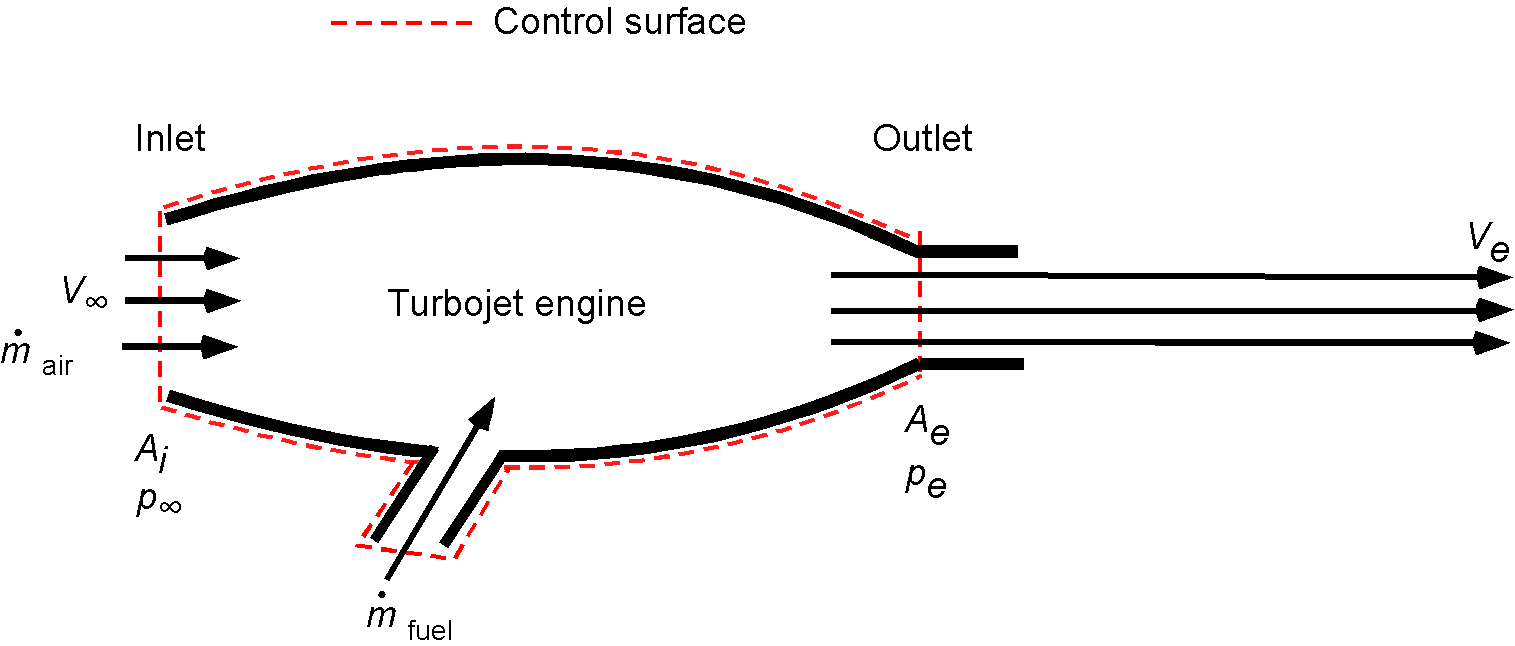
A control volume approach for analyzing a turbojet engine, which works on the air to increase its momentum in the downstream direction. According to Newton’s third law, the thrust is directed upstream.

The mass flow of air into the engine will be

(55) $\begin{equation*} \overbigdot{m}_{\rm air} = \varrho_{\infty} V_{\infty} A_i \end{equation*}$

where $A_i$ is the inlet area, and the mass flow rate of fuel is ${\overbigdot{m}_{\rm fuel}}$ . Therefore, the thrust is

(56) $\begin{equation*} T = (\overbigdot{m}_{\rm air} + \overbigdot{m}_{\rm fuel} ) V_e - \overbigdot{m}_{\rm air} V_{\infty} + ( p_e - p_{\infty} ) A_e ) \end{equation*}$

with $A_e$ as the exit area and $V_e$ as the exit or “jet” velocity. The pressure term in Eq. 56 is relatively small compared to the change in momentum of the flow and so may be neglected, i.e.,

(57) $\begin{equation*} T = (\overbigdot{m}_{\rm air} + \overbigdot{m}_{\rm fuel} ) V_e - \overbigdot{m}_{\rm air} V_{\infty} \end{equation*}$

If the mass flow of the fuel (small) is neglected in comparison to the mass flow rate of air (high), then

(58) $\begin{equation*} T = \overbigdot{m}_{\rm air} V_j - \overbigdot{m}_{\rm air} V_{\infty} = \overbigdot{m} \left(V_j - V_{\infty} \right) \end{equation*}$

Using the principle of conservation of energy, the propulsive efficiency can be defined as

(59) $\begin{equation*} \eta_p = \frac{\mbox{\small Useful power produced}}{\mbox{\small Total power expended }} = \frac{T \, V_{\infty}}{ T \, V_{\infty} + \frac{1}{2} \overbigdot{m} \left( V_j - V_{\infty} \right)^2} \end{equation*}$

which shows that losses appear as a gain in kinetic energy in the downstream jet flow. Substituting for the thrust gives

(60) $\begin{equation*} \eta_p= \frac{\overbigdot{m} \left( V_j - V_{\infty} \right) V_{\infty}}{ \overbigdot{m} \left( V_j - V_{\infty} \right) V_{\infty} + \frac{1}{2} \overbigdot{m} \left( V_j - V_{\infty} \right)^2} = \frac{2}{1 + \left( \displaystyle{\frac{V_j}{V_{\infty} }}\right) } \end{equation*}$

where to be meaningful $V_j > V_{\infty}$ . Notice that a low value of $V_j$ for a given thrust and, hence, higher propulsive efficiency can be achieved by having a significantly high mass flow rate, $\overbigdot{m}$ , through the engine. Therefore, even with this relatively simple analysis, it can be concluded that it is more efficient to generate thrust by accelerating a large air volume (mass flow rate) at a lower $V_j$ than by accelerating a smaller air volume (mass flow rate) at a higher $V_j$ .

Forces on a Two-Dimensional body

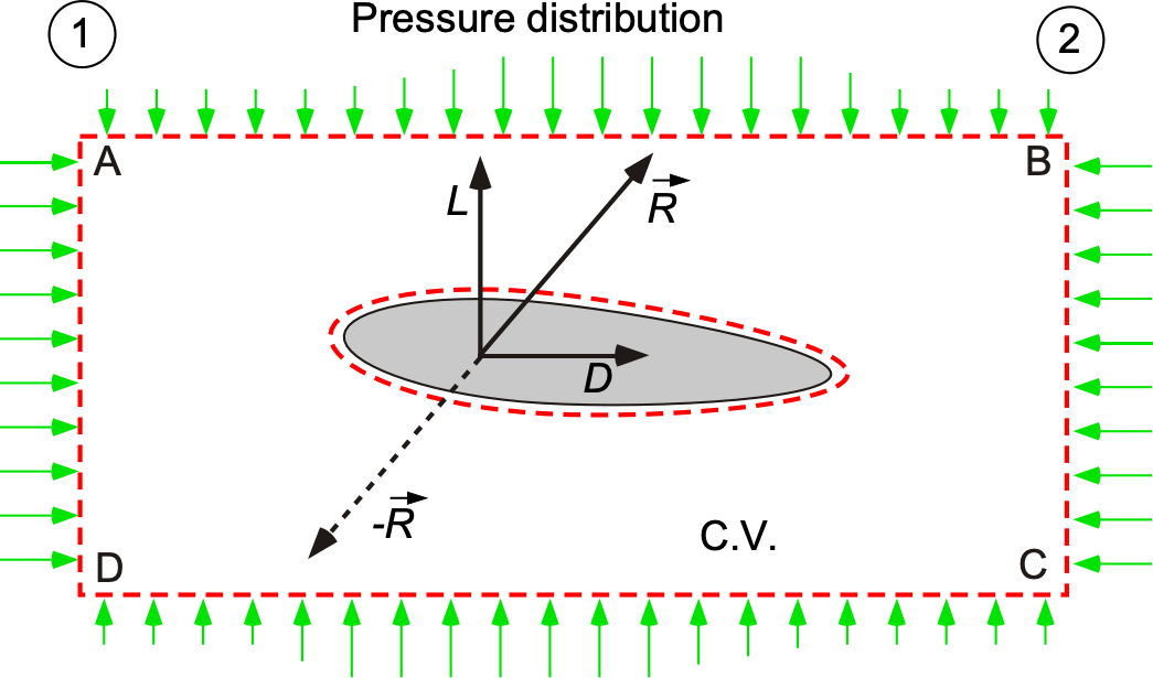
The conservation laws can be used to determine the drag of a two-dimensional body in terms of off-surface fluid properties, e.g., the force on a body in a wind tunnel. Consider the physical problem of a body immersed in a fluid flow, as shown in Figure 18. The fluid exerts pressure and viscous forces on the body, which are sources of the resultant force $R$ and, hence, of the lift $L$ and the drag $D$ . Physically, because of these effects, a wake with a lower flow velocity will form downstream of the body. The objective is to use the fluid equations of motion (in this case, the continuity and momentum equations) to calculate the force on the body.

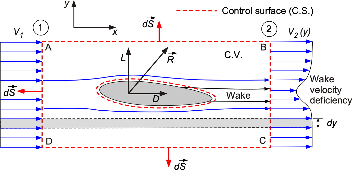
The upstream and downstream sections, labeled 1 and 2, and the top and bottom sides bound the control volume. The top and bottom sides of the control volume are considered sufficiently far from the body that they are in the freestream and, therefore, are streamlines to the flow; i.e., there will be no flow over these boundaries. These boundaries, for example, could be the floor and ceiling of a wind tunnel. Remember that $d\vec{S}$ points out of the control volume by convention. The upstream or freestream (undisturbed) velocity is ${V_1}$ = constant = ${V_{\infty}}$ . Because of viscosity, a wake of reduced velocity or diminished flow exists behind the body; this gives a wake region a velocity profile in which $V_2 < V_\infty$ .

Consider the forces on the fluid in the control volume. They stem from two sources:

The net effect of the pressure distribution over the control volume, i.e., over the surface ABCD, then
(61) $\begin{equation*} \mbox{\small Net pressure force} = -\iint_{\rm ABCD} \, p \, d\vec{S} \end{equation*}$
The reaction of the surface forces on the body, i.e., those forces produced over the inner part of the control volume as created by the body, i.e., $-\vec{R}$ , by Newton’s 3rd law.

Remember that the flow will exert pressure and shear forces on the body, resulting in a resultant force, $\vec{R}$ . This means, by Newton’s third law, that the airfoil will exert a force $-\vec{R}$ on the fluid within the control volume. Therefore, the total force on the fluid volume is the sum of the pressure forces on the control surface and the reaction force of the body on the fluid, i.e.,

(62) $\begin{equation*} \mbox{\small Net force} = -\iint_{\rm ABCD} p \, d\vec{S} - \vec{R} \end{equation*}$

and from the conservation of momentum equation, then

(63) $\begin{equation*} -\iint_{\rm ABCD} p \, d\vec{S} - \vec{R} = \frac{d}{dt}\oiiint_{\rm C.V.} \varrho\vec{V} d {\cal{V}} + \iint_{\rm ABCD} \left(\varrho \, \vec{V} \bigcdot d\vec{S} \right) \vec{V} \end{equation*}$

For steady flow $\partial ({\rm everything})/ \partial t = 0$ , so that this latter equation is simplified to

(64) $\begin{equation*} \vec{R} = -\iint_{\rm ABCD} \left(\varrho\vec{V}\bigcdot d\vec{S}\right) \vec{V} -\iint_{\rm ABCD} p \, d\vec{S} \end{equation*}$

Notice that this latter equation is a vector equation.

Drag Force

To find the drag, the ${x}$ -component of this latter equation is needed, noting that ${V_{\infty}}$ and ${V_2}$ are the inflow and outflow velocities in the ${x}$ -direction and that the ${x}$ -component of $R$ is the drag on the section, i.e., $D$ per unit span. The pressures upstream and downstream are equal, i.e., there is no longitudinal pressure gradient, so that

(65) $\begin{equation*} \iint_{\rm AD} p \, d\vec{S} = \iint_{\rm CB} p \, d\vec{S} \end{equation*}$

Therefore, the force on the fluid and drag on the body can be expressed only in terms of the ${u}$ velocity profiles upstream and downstream, i.e.,

(66) $\begin{equation*} D = -\iint_{\rm ABCD} \left(\varrho\vec{V}\bigcdot d\vec{S} \right) u \end{equation*}$

and so this integral becomes a one-dimensional integral (noting the signs on the components), i.e.,

(67) $\begin{equation*} D = -\bigg( - \int_{D}^{A} \varrho_{_{\infty}} V_{\infty}^{2} dy + \int_{C}^{B}\varrho_{2}V_{2}^{2}dy \bigg) = \int_{D}^{A}\varrho_{_{\infty}}V_{\infty}^{2}dy - \int_{C}^{B}\varrho_{2} V_{2}^{2}dy \end{equation*}$

The continuity equation can also be applied to the control volume, i.e., based on the principle of conservation of mass, then

(68) $\begin{equation*} \int_{D}^{A}\varrho_{_{\infty}}V_{1}dy = \int_{C}^{B} \varrho_{2} V_{2} dy \end{equation*}$

Multiplying by ${V_{\infty}}$ in this case (which is a constant) gives

(69) $\begin{equation*} \int_{D}^{A}\varrho_{_{\infty}}V_{\infty}^2 dy = \int_{C}^{B} \varrho_{2} V_{2} V_{\infty} dy \end{equation*}$

Substituting back into the expression for $D$ gives

(70) $\begin{eqnarray*} D & = & \int_{D}^{A}\varrho_{_{\infty}}V_{\infty}^{2}dy - \int_{C}^{B}\varrho_{2} V_{2}^{2}dy = \int_{C}^{B} \varrho_{2} V_{2} V_{\infty}dy - \int_{C}^{B}\varrho_{2}V_{2}^{2}dy \\ [6pt] & = & \int_{C}^{B}\varrho_{2}V_{2} \left(V_{\infty} - V_{2}\right)dy \end{eqnarray*}$

This latter expression gives the drag of a two-dimensional body in terms of ${V_{\infty}}$ and the flowfield properties $\varrho_2$ and ${V_2}$ , evaluated across a vertical plane downstream of the body.

Notice that $V_{\infty} - V_2$ is the velocity deficiency or decrement at a given station (or section) in the downstream wake. Also, $\varrho_{2}V_{2}$ is the mass flux, so the product $\varrho_{2}V_{2}(V_{\infty}-V_{2})$ gives the decrement in momentum. The integral of this expression leads to the total decrement in momentum behind the body and, hence, the drag of the section. If $\varrho$ = constant, then things can be simplified even further to get

(71) $\begin{equation*} D =\varrho\int_{C}^{B}V_{2}\left(V_{\infty} -V_{2}\right) dy =\varrho_{\infty} \int_{C}^{B}V_{2}\left(V_{\infty}-V_{2}\right) dy \end{equation*}$

However, caution is needed, as this approach is effective only when flow separation or turbulence around the body is minimal. If there are significant wake losses because of viscous effects from turbulent eddies, the drag will be underestimated.

This latter technique is frequently employed in wind tunnel testing to measure forces on relatively streamlined bodies; the velocities downstream of the body or airfoil are measured using a wake rake. This rake is, in fact, an array of Pitot tubes used to measure dynamic pressure and flow velocity in the wake. The momentum deficit is measured at discrete points in the wake, so that the drag per unit span is

(72) $\begin{equation*} D \approx \varrho_{_{\infty}} \sum_{i=1}^{N} V_2(x, y_i) \bigg( V_\infty - V_2(x, y_i) \bigg) \Delta y \end{equation*}$

where $V_2(x, y_i)$ is the velocity at the $i$ -th point in the wake, and $\Delta y$ is the spacing between the measurement points; $\Delta y$ does not have to be uniform. The values would be measured for each test point, e.g., different flow speeds and angles of attack.

Lift Force

Consider now how to measure the lift on the body, which is the force in the ${y}$ direction. The lift on the C.V. is calculated as the net vertical force resulting from the pressure difference between the surface AB (the ceiling) and CD (the floor), i.e.,

(73) $\begin{equation*} L = \iint_{_{\text{fl}}} p \, dS - \iint_{_{\text{ce}}} p \, dS = \iint_{\text{CD}} p \, dS - \iint_{\text{AB}} p \, dS \end{equation*}$

as illustrated in Figure 19, where $p_{_{\text{ce}}}(x)$ is the measured pressure distribution (using pressure taps) along the ceiling, and $p_{_{\text{fl}}}(x)$ is the pressure distribution along the floor. Again, while the floor and ceiling are streamlines to the flow there can be a pressure distribution along their lengths from the presence of the body.

Lift on a body can be determined from the pressure distributions on the floor and ceiling of the wind tunnel.

The sectional lift per unit span is obtained using a one-dimensional pressure integral along the length of the control volume, i.e.,

(74) $\begin{equation*} L = \int_{x_1}^{x_2} \bigg( p_{_{\text{fl}}}(x) - p_{_{\text{ce}}}(x) \bigg) dx \end{equation*}$

$x_1$ would be located at the start of the test section, and $x_2$ will be at or near the end. Each pressure tap would be connected to a pressure measurement system. Because the pressure will be measured at discrete points along the wind tunnel walls, the lift per unit span is given as

(75) $\begin{equation*} L \approx \sum_{i=1}^{N} \bigg( p_{_{\text{fl}}}(x_i) - p_{_{\text{ce}}}(x_i) \bigg) \Delta x \end{equation*}$

where $x_i$ represents the measurement locations along the wind tunnel, and $\Delta x$ is the spacing between measurement points; $\Delta x$ can be non-nuniform. This sum is just the area under the $\Delta$ pressure curve between the floor and the ceiling along the length of the test section.

Historical Context: NACA and Abbott & Von Doenhoff

The integral method was extensively used by NACA researchers, notably Ira Abbot and Albert von Doenhoff, whose influential 1940s work was published as “Theory of Wing Sections & Summary of Airfoil Data.” Their approach inferred forces from test-section wall-pressure distributions and wake surveys, thereby eliminating the need for direct surface measurements, such as pressures on each airfoil. This method enabled the testing and comparison of more than 200 airfoil sections, significantly benefiting the aeronautics industry by providing a comprehensive catalog of airfoil shapes that could be selected to meet specific aerodynamic requirements.

Firefighting Drone

It has been proposed that a quad-rotor drone can fight a high-rise fire by supporting a free-hanging hose supplied by a ground-based pump. At first glance, the idea appears interesting and plausible. A ground-based pump provides the pressure needed to lift the water to the drone, so it may seem that the drone only needs to position the nozzle and direct water onto the fire. But perhaps there is more to understand. The good news is that the details of this problem can be adequately assessed using the application of the laws of physics and the conservation laws of fluid mechanics, which allow the forces acting on the drone to lift and deliver the water to be estimated, along with the pumping power to produce the needed hydrostatic pressure head and the discharge of water from the nozzle toward the fire.

Consider a hovering drone supporting a free-hanging firefighting hose with water supplied by a ground-based pump, as shown in Figure 20. The water in the suspended portion of the hose has a weight that must be carried as a tension force at the top of the hose, and so by a thrust created by the drone’s rotors. The hose can be assumed to have an internal diameter $D$ and to hang a distance $L$ below the drone. If the building has $p$ stories and a representative story height is 3 m, then $L = 3 \, p$ . The mass of water contained in the suspended hose is

(76) $\begin{equation*} m_w = \varrho_w \, A \, L = \varrho_w \left( \frac{\pi \, D^2}{4} \right) L \end{equation*}$

and the corresponding weight of the water is

(77) $\begin{equation*} W_w = \varrho_w \, g \, A \, L = m_w \, g \end{equation*}$

The weight of water in the hose is present whether or not water is flowing.

A proposed firefighting drone could be helpful, but does it make physical sense? The answer lies in the conservation laws of fluid mechanics.

If the hose is free-hanging, the weight of the water must be supported by tension force at the top of the hose and so by the thrust produced by the drone’s rotors. The hose itself also has weight; if the dry hose mass per unit length is $\mu_h$ , then the weight of the hose over the suspended length is

(78) $\begin{equation*} W_h = \mu_h \, g \, L \end{equation*}$

Therefore, the force that the drone must overcome (besides its own weight) is

(79) $\begin{equation*} T_{\text{drone}} = W_w + W_h = g \, L\left(\varrho_w \, A + \mu_h\right) = g \, L\left(\varrho_w \frac{\pi \, D^2}{4} + \mu_h \right) \end{equation*}$

To estimate the approximate magnitude of this force, which is key to determining the practical feasibility of the system, one can assume a modest size fire hose with an internal diameter of $D$ = 0.045 m (about 1.7 inches) and a water density of $\varrho_w$ = 1,000 kg/m $^{3}$ . For this hose, the cross-sectional area is $A = \dfrac{\pi (0.045)^2}{4} =$ 1.59 $\times$ 10 $^{-3}$ m $^{2}$ , so the water mass per unit length in the hose is $\varrho_w \, A =$ 1.59 kg/m, and the corresponding water weight per unit length is

(80) $\begin{equation*} w_w = \varrho_w \, g \, A = 15.6~\mathrm{N/m} \end{equation*}$

A pressurized fire hose is heavy; a representative dry mass per unit length is $\mu_h \approx$ 1.0 kg/m, giving a weight per unit length of

(81) $\begin{equation*} w_h = \mu_h \, g = 9.81~\mathrm{N/m} \end{equation*}$

Therefore, the combined suspended weight per unit length (hose plus contained water) is

(82) $\begin{equation*} w_{\text{total}} = w_w + w_h \approx 25.4~\mathrm{N/m} \end{equation*}$

Consider a 15-story building, so that $p$ = 15 and $L = 3 \, p$ = 45 m. The quasi-static thrust to be produced by the drone is then

(83) $\begin{equation*} T_{\text{drone}} \approx w_{\text{total}} \, L = 25.4 \times 45 = 1.14\times 10^{3}~\mathrm{N} \end{equation*}$

which corresponds to an equivalent supported mass of

(84) $\begin{equation*} m_{\text{equiv}} = \frac{T_{\text{drone}}}{g} \approx \frac{1.14\times 10^{3}}{9.81} \approx 116~\mathrm{kg} \end{equation*}$

In practice, wind loading and flow transients require additional margin. Using a modest factor of 1.5 yields a design load of approximately 1.7 $\times$ 10 $^{3}$ N, or about 175 kg equivalent mass, before accounting for fittings and nozzle hardware.

The next issue is to assess the role of the ground-based pump and the forces generated at the nozzle. In addition to the static suspended load, the water exiting the nozzle toward the fire produces a reaction force associated with the rate of change of the flow’s momentum. For a control volume drawn around the nozzle, conservation of linear momentum gives the force exerted on the fluid as

(85) $\begin{equation*} \vec{F}_{\text{on fluid}} = \overbigdot{m}\,(\vec{V}_{\text{out}}-\vec{V}_{\text{in}}) + \int_A (p - p_\infty)\,d\vec{S} \end{equation*}$

where $\overbigdot{m}$ is the mass flow rate, $\vec{V}_{\text{in}}$ and $\vec{V}_{\text{out}}$ are the inlet and outlet velocities, and the surface integral represents the pressure-thrust contribution. For a firefighting nozzle discharging to the atmosphere, $p_{\text{out}} \approx p_\infty$ , and if the inlet velocity is small compared to the exit velocity, i.e., $V_{\text{in}} \ll V_{\text{out}}$ , then the pressure and inlet momentum terms are negligible. Under these assumptions, the reaction force magnitude acting on the nozzle (and hence on the drone) reduces to the momentum-flux form

(86) $\begin{equation*} F_{\text{jet}} = \overbigdot{m} \, V_j = \varrho_w \, Q \, V_j \end{equation*}$

where $V_j$ is the jet exit speed. For a representative volumetric flow rate of $Q$ = 0.010 m $^{3}$ /s (10.0 L/s, 158 USgal/min), the corresponding mass flow rate is

(87) $\begin{equation*} \overbigdot{m} = \varrho_w \, Q = 1,000 \times 0.010 = 10.0~\mathrm{kg/s} \end{equation*}$

For representative nozzle exit speeds in the range $V_j$ = 25–40 m/s, the resulting reaction force is $F_{\text{jet}} = \overbigdot{m} \, V_j \approx$ 250–400 N. Because the jet is directed toward the fire, this reaction force acts primarily in the horizontal direction. The drone must therefore tilt its rotor thrust vector to generate a horizontal component equal to $F_{\text{jet}}$ , while maintaining a vertical component equal to the suspended load. If $T_{\text{drone}} = W_w + W_h$ denotes the tension at the top of the hose because of the weight, then the total rotor thrust required is

(88) $\begin{equation*} T = \sqrt{T_{\text{drone}}^{\,2} + F_{\text{jet}}^{\,2}} \end{equation*}$

and the corresponding tilt angle of the thrust vector away from vertical is

(89) $\begin{equation*} \theta = \tan^{-1}\!\left(\frac{F_{\text{jet}}}{T_{\text{drone}}}\right) \end{equation*}$

For the present example with $T_{\text{drone}} \approx$ 1.14 $\times$ 10 $^{3}$ N and $F_{\text{jet}} \approx$ 250–400 N, the required thrust magnitude increases only modestly, but the thrust vector must be tilted by approximately $\theta \approx$ 12 $^\circ$ –19 $^\circ$ . This tilt reduces the vertical lift component available to support the suspended hose, thereby requiring a corresponding increase in total rotor thrust by a factor of $1/\cos\theta$ ; the corresponding power for flight would increase by $(1/\cos \theta)^{3/2}.$

The next issue is to assess the role of the ground-based pump in sustaining the prescribed flow rate and jet. For steady vertical flow, the static pressure rise (hydrostatic head) required to elevate the water through a height $L$ is $\Delta p_{\text{static}} = \varrho_w \, g \, L$ . For $L$ = 45 m then

(90) $\begin{equation*} \Delta p_{\text{static}} = 1,000 \times 9.81 \times 45 = 4.41\times 10^{5}~\mathrm{Pa} = 441~\mathrm{kPa} \end{equation*}$

This pressure rise represents an energy requirement that appears as a pumping power; it does not provide an external force that supports the weight of the water in the suspended hose.

For a volumetric flow rate $Q$ = 0.010 m $^{3}$ /s (10.0 L/s, 158 USgal/min), the corresponding hydraulic power required to overcome the hydrostatic head is $P_{\text{static}} = \Delta p_{\text{static}} \, Q$ . For this flow rate, then

(91) $\begin{equation*} P_{\text{static}} = (4.41\times 10^{5}) \times 0.010 = 4.41\times 10^{3}~\mathrm{W} = 4.41~\mathrm{kW} \end{equation*}$

Assuming a representative pumping efficiency of $\eta_p = 0.70$ , the corresponding shaft power required to overcome the hydrostatic head alone is

(92) $\begin{equation*} P_{\text{shaft,static}} = \frac{P_{\text{static}}}{\eta_p} \approx \frac{4.41}{0.70} \approx 6.3~\mathrm{kW} \end{equation*}$

In addition to lifting the water column, the pump must also supply the kinetic energy of the water jet discharged from the nozzle. Neglecting inlet velocity and internal nozzle losses, the ideal pressure drop required to form a jet of exit speed $V_j$ is

(93) $\begin{equation*} \Delta p_{\text{nozzle}} \approx \frac{1}{2}\,\varrho_w \, V_j^{\,2} \end{equation*}$

and the corresponding hydraulic jet power is

(94) $\begin{equation*} P_{\text{jet}} = \Delta p_{\text{nozzle}} \, Q = \frac{1}{2}\,\varrho_w \, Q \, V_j^{\,2} \end{equation*}$

For representative nozzle exit speeds in the range $V_j$ = 25–40 m/s, this gives $\Delta p_{\text{nozzle}} \approx$ 0.31–0.80 MPa and $P_{\text{jet}} \approx$ 3.1–8.0 kW, so that the corresponding shaft power associated with the jet is approximately 4.4–11.4 kW. Even neglecting hose friction and minor losses, the total pump shaft power required to sustain both the vertical water column and the jet is of the order $P_{\text{shaft,total}} \approx$ 10–18 kW (13–24 hp) per drone.

Therefore, when examined from first principles, the answer to the original question becomes clear. A drone supporting a free-hanging firefighting hose must carry the weight of the hose and the water it contains, regardless of where the pump is located and how much power it can produce. For a 15-story building, the suspended load alone exceeds what is currently practical for conventional multirotor drones.

Compressible Flow in a Converging-Diverging Nozzle

In many applications of a Venturi, the flow speeds remain low enough that density changes are negligible, and the incompressible form of Bernoulli’s equation applies. However, if the pressure ratio across a converging-diverging duct becomes sufficiently large, the flow can become appreciably compressible, and the throat may reach the sonic condition, i.e., ${M = 1}$ . Under these circumstances, the device is more properly regarded as a converging-diverging nozzle, as shown in Figure 21, rather than a Venturi used purely as a flow meter.

Compressible flow through a nozzle can be analyzed using the standard isentropic equations of fluid dynamics.

For steady, one-dimensional flow, the continuity equation still requires that the mass flow rate be constant, i.e.,

(95) $\begin{equation*} \overbigdot{m} = \varrho \, A \, V = \mbox{\small constant} \end{equation*}$

However, $\varrho$ is no longer constant, and so the volumetric flow rate $Q = A \, V$ is not constant along the nozzle. For adiabatic flow with no shaft work, the appropriate energy relation is expressed in terms of stagnation (total) enthalpy,

(96) $\begin{equation*} h_0 = h + \frac{V^2}{2} = \mbox{\small constant} \end{equation*}$

For a perfect gas with constant specific heats, $h = c_p T$ , so this may be written in terms of the stagnation temperature $T_0$ as

(97) $\begin{equation*} T_0 = T \left( 1 + \frac{\gamma - 1}{2} \, M^2 \right) \end{equation*}$

where $M = V/a$ is the Mach number and $a = \sqrt{\gamma \, R \, T}$ is the local speed of sound. If the flow is isentropic, so that no shocks are present and viscous dissipation is negligible, then the stagnation pressure is also constant, and the static-to-stagnation relations are

(98) $\begin{equation*} \frac{p_0}{p} = \left( 1 + \frac{\gamma - 1}{2} \, M^2 \right)^{\frac{\gamma}{\gamma - 1}} \qquad \text{and} \qquad \frac{\varrho_0}{\varrho} = \left( 1 + \frac{\gamma - 1}{2} \, M^2 \right)^{\frac{1}{\gamma - 1}} \end{equation*}$

A key result for compressible nozzle flow is the area-Mach number relation, i.e.,

(99) $\begin{equation*} \frac{A}{A^*} = \frac{1}{M} \left[ \frac{2}{\gamma + 1} \left( 1 + \frac{\gamma - 1}{2} \, M^2 \right) \right]^{\frac{\gamma + 1}{2(\gamma - 1)}} \end{equation*}$

where $A^*$ is the critical area at which ${M = 1}$ . This relation implies that a given area ratio $A/A^*$ generally corresponds to two possible solutions, one subsonic and one supersonic. As back pressure decreases, the Mach number at the throat increases. When the throat reaches the sonic condition ${M = 1}$ , the flow is said to be choked. Under choked conditions, the mass flow rate reaches a maximum for the given upstream stagnation state $(p_0, T_0)$ , and further reductions in back pressure do not increase $\overbigdot{m}$ . The choked mass flow rate is

(100) $\begin{equation*} \overbigdot{m}_{\max} = A^* p_0 \sqrt{\frac{\gamma}{R \, T_0}} \left( \frac{2}{\gamma + 1} \right)^{\frac{\gamma + 1}{2(\gamma - 1)}} \end{equation*}$

If the back pressure is low enough, the flow accelerates to supersonic speed in the diverging section. If the back pressure is not low enough to support fully supersonic flow, a normal shock may stand in the diverging section, causing an abrupt transition from supersonic to subsonic flow and a substantial loss of stagnation pressure. Depending on the back pressure, a converging-diverging nozzle may therefore operate in one of several regimes: entirely subsonic flow, choked flow with a normal shock in the diverging section, or fully supersonic expansion to the exit.

Summary & Closure

Many fluid-flow problems can be analyzed using the continuity and momentum equations in integral form, along with the energy equation in the surrogate form of the Bernoulli equation. All three conservation principles will be required for most practical problems, along with the complete energy equation and the equation of state when compressibility effects are present. The momentum equation is always required when calculating forces. Problems that can be assumed to be steady, inviscid, and incompressible are the easiest to understand and predict; accordingly, some examples have been discussed and solved in this chapter. The experience gained from solving these exemplary fluid-flow problems increases confidence in analyzing more complex problems, such as those involving unsteadiness and compressibility effects.

5-Question Self-Assessment Quickquiz

For Further Thought or Discussion

Why is the flow through a rapidly converging or expanding Venturi (or duct) more difficult to justify as one-dimensional?
What happens when an aircraft flies at higher Mach numbers? Does Bernoulli’s equation apply?
Who was Henri Pitot? What did he do besides invent the Pitot tube?
Using a drinking straw and a ruler, explain how you would measure the flow velocity in a water channel.
What happens in the throat of a Venturi as the flow speed becomes subsonic and then supersonic?
Think about some aeronautical problems that cannot be tackled using the conservation principles in integral form.
It is proposed that the drag of a circular cylinder is to be measured in a wind tunnel using the momentum deficiency technique. What is the concern here, and why?
Why does a balloon filled with helium deflate more quickly than a balloon filled with air?
If the drag on a body can be measured using a momentum integral method, how can the lift on the body be measured?

Additional Online Resources

Explore some of these additional online resources to help understand the application of the conservation laws when applied to simple fluid flow problems:

Explore this interactive simulation of flow through a pipe.
Video of worked example problems using the conservation laws.
View this video for a simple experimental demonstration of a U-tube manometer.
This Pitot Static System Simulator allows you to visualize the Pitot static system on an airplane under varying atmospheric conditions and what happens when system parts become blocked.

Sadler, D. R. (2005). "Interpretations of Criteria-Based Assessment and Grading in Higher Education." Assessment and Evaluation in Higher Education, 30 (2), 175–194. ↵
. The diameter of such holes should be less than 0.5 mm or 20-thousandths of an inch. ↵
Evangelista Torricelli's original derivation can be found in the second book "De motu aquarum" of his "Opera Geometrica." See also: A. Malcherek, "History of the Torricelli Principle and a New Outflow Theory," Journal of Hydraulic Engineering, 142 (11), 1–7, 2016. ↵

License

Icon for the Creative Commons Attribution-NonCommercial-NoDerivatives 4.0 International License

Introduction to Aerospace Flight Vehicles Copyright © 2022–2026 by J. Gordon Leishman is licensed under a Creative Commons Attribution-NonCommercial-NoDerivatives 4.0 International License, except where otherwise noted.

Digital Object Identifier (DOI)

https://doi.org/https://doi.org/10.15394/eaglepub.2022.1066.n19