Airspeed Definitions & Measurement

J. Gordon Leishman

doi:https://doi.org/10.15394/eaglepub.2022.1066.n29

41 Airspeed Definitions & Measurement

Introduction

Knowing how fast an aircraft travels through the air is fundamental to both piloting and engineering because it directly governs the aerodynamic forces acting on the vehicle and, therefore, its overall performance. Aircraft performance characteristics are generally expressed in terms of airspeed and/or Mach number, together with flight altitude and aircraft weight, all of which determine lift, drag, and the corresponding power or thrust required. However, determining an aircraft’s airspeed requires considerable care and a sound understanding of both aerodynamic principles and measurement techniques.

Pilots are often most directly concerned with the indicated airspeed (IAS), which is read from the airspeed indicator (ASI) or electronic flight display (EFIS) in the cockpit. When the IAS is corrected for instrument and position errors, the result is the calibrated airspeed (CAS). A further correction for compressibility effects yields the equivalent airspeed (EAS), a significant airspeed because it is directly proportional to the dynamic pressure acting on the airplane. For this reason, many critical airspeeds are most naturally referenced in terms of EAS. Engineers are also concerned with the aircraft’s true airspeed (TAS) in undisturbed air, the infamous “ ${V_{\infty}},$ ”which generally differs from IAS, CAS, and EAS. True airspeed, together with ground speed (which accounts for wind effects), is also required by pilots for navigation. Therefore, to avoid confusion and possible misinterpretation, the various definitions of airspeed and the physical basis of their measurement must be clearly understood, as well as how these quantities are used in both engineering analysis and aviation practice.

Learning Objectives

Understand the aerodynamic principles associated with airspeed measurement.
Know the difference between indicated, equivalent, calibrated, and true airspeeds.
Be able to calculate the true airspeed of an aircraft.
Know how to calculate airspeed at higher Mach numbers.
Learning about new approaches to airspeed measurement using optical methods.

Airspeed & Mach Number

When evaluating a flight vehicle’s performance, its airspeed capabilities are fundamental. In engineering terms, this refers to the true airspeed of the aircraft relative to the surrounding air, denoted by ${V_{\infty}}$ . Unlike a terrestrial vehicle, where speed can be determined directly from distance traveled over the ground in a given time, an aircraft’s airspeed cannot be measured this way. Instead, its speed, called airspeed, must be determined from pneumatic measurements, such as those obtained using Pitot probes, and the true speed through the air must be inferred using principles of aerodynamics, hydrostatics, and thermodynamics.

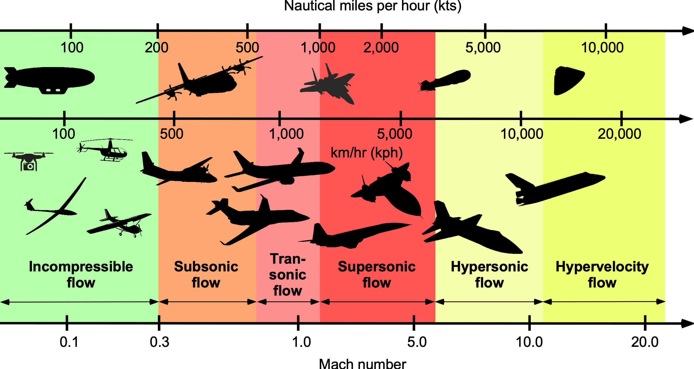
A flight vehicle’s airspeed is often classified in terms of its corresponding Mach number, as shown in Figure 1. Recall that the Mach number is defined as the ratio of airspeed to the local speed of sound, so that

(1) $\begin{equation*} M_{\infty} = \frac{V_{\infty}}{a_{\infty}} \end{equation*}$

where ${V_{\infty}}$ is the true airspeed and $a_{\infty}$ is the freestream speed of sound at the prevailing atmospheric conditions.

Mach number is one of the most useful parameters for characterizing the aerodynamic behavior of a flight vehicle across different speed regimes.

The speed of sound depends on the ambient air temperature, $T_{\infty}$ , at any altitude, i.e.,

(2) $\begin{equation*} a_{\infty} = \sqrt{\gamma R T_{\infty}} \end{equation*}$

Therefore, for a given true airspeed, the Mach number increases with altitude as the atmospheric temperature decreases. In engineering practice, the International Standard Atmosphere (ISA) is typically used to define these properties unless otherwise specified, providing a consistent basis for calculations, instrument calibration, and performance comparisons.

Flight in the low subsonic regime corresponds approximately to $M_{\infty} \ approx 1$ , typically up to about 3, depending on the vehicle design. In this regime, shock waves significantly affect the flow field, including the pressure distribution around Pitot probes and other measurement devices. Consequently, thermodynamic relationships are essential for determining the aircraft’s true airspeed from measured pressures.

Definitions of Airspeeds

Several speeds may be used in aircraft operations, which must now be defined. For example, the aircraft’s speed over the ground differs from its true airspeed. This is because the ground speed depends on the relative magnitude and direction of the winds in the air mass in the direction of flight. Additionally, the speed read by an airspeed indicator (or its EFIS equivalent) is not the aircraft’s actual or “true” speed, nor is it its ground speed. This may sound confusing, and it certainly is to most new engineers; therefore, the various airspeeds used in aircraft must be understood.

What Does an ASI Measure?

It is best to understand precisely what an airspeed indicator (ASI) measures. An ASI, as shown in Figure 2, is one of the most fundamental instruments used in flight, and the readings from an ASI are used not only for piloting but also for engineering purposes. An ASI is a pressure-measuring (pneumatic) instrument that responds to dynamic pressure or “ $q$ ” variations with a scale calibrated in speed units. Recall that freestream dynamic pressure is given by $q_\infty = \dfrac{1}{2} \, \varrho_\infty \, V_\infty^2$ , where $\varrho_\infty$ is the ambient air density and $V_\infty$ is the true airspeed. The ASI is calibrated to read airspeed, usually in units of “knots” (kts), which means nautical miles per hour. Units of “knots” are used universally in aviation, but some ASIs may be calibrated in units of kilometers per hour (km/h, or kph).

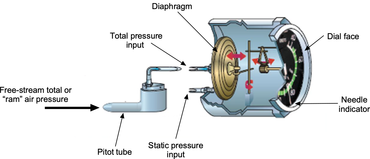
An airspeed indicator is calibrated in speed units but responds to dynamic pressure. The pressure source is typically a pitot-static probe, which consists of a pitot probe and a static vent.

Recall that dynamic pressure is the difference between the total or stagnation pressure $p^*$ (the “ram” pressure) and the static pressure $p_s$ , i.e., $q = p^* - p_s$ . Sometimes, a Pitot-static probe is used to measure dynamic pressure; at other times, a separate total-pressure probe (which measures $p^*$ ) and a static-pressure vent placed on the aircraft’s surface (which measures $p_s$ ) are employed. In either case, the measured pressure difference is the dynamic pressure, $q$ , which the ASI responds to by design.

Airspeed Analysis

Consider flight at low Mach numbers, where the flow can be treated as incompressible. If the total (stagnation) pressure is denoted as $p^*$ , then the use of Bernoulli’s equation gives

(3) $\begin{equation*} p_s + \frac{1}{2} \varrho_{\infty} \, V_{\infty}^2 = p^* \end{equation*}$

Rearranging this equation gives the true airspeed (TAS), i.e.,

(4) $\begin{equation*} V_{\rm {\tiny TAS}} = \sqrt{ \frac{p^* - p_s}{2 \, \varrho_{\infty}}} = \sqrt{\frac{\Delta p}{2 \, \varrho_{\infty}}} \end{equation*}$

Introducing the density ratio $\sigma = \varrho_{\infty}/\varrho_0$ gives

(5) $\begin{equation*} V_{\rm {\tiny TAS}} = \sqrt{\frac{\Delta p}{2 \, \varrho_0}} \, \frac{1}{\sqrt{\sigma}} \end{equation*}$

which is exact if the density $\varrho_{\infty}$ and the measured value of $\Delta p$ are known.

Of course, this equation is not especially convenient for finding TAS because $\varrho_{\infty}$ depends on pressure altitude and temperature. Also, a speed scale on the ASI must be associated with any given $\Delta p$ , so a formal calibration is required. It will also be apparent that the ASI scale is nonlinear because dynamic pressure varies as the square of airspeed.

Basis of Calibration

To resolve these issues, the airspeed measurement is referenced to mean sea level (MSL) density by calibrating the ASI assuming $\varrho_{\infty} = \varrho_0$ . At low Mach numbers, calibrated airspeed (CAS) and equivalent airspeed (EAS) are essentially the same, so that the ASI may be interpreted directly in terms of EAS. The corresponding airspeed is the equivalent airspeed (EAS), i.e.,

(6) $\begin{equation*} V_{\rm {\tiny EAS}} = \sqrt{ \frac{p^* - p_s }{2 \, \varrho_0} } = \sqrt{ \frac{\Delta p}{2 \, \varrho_0} } \end{equation*}$

so that

(7) $\begin{equation*} \frac{1}{2} \, \varrho_0 \, V_{\rm {\tiny EAS}}^2 = \frac{1}{2} \, \varrho_{\infty} \, V_{\rm {\tiny TAS}}^2 \end{equation*}$

Hence, the true airspeed is obtained from a calculation using

(8) $\begin{equation*} V_{\rm {\tiny TAS}} = \frac{V_{\rm {\tiny EAS}}}{\sqrt{\sigma}}, \qquad \sigma = \frac{\varrho}{\varrho_0} \end{equation*}$

which requires the value of $\sigma$ to be evaluated.

Finding Air Density

Determining $\sigma$ requires measurements of the pressure altitude, $h_p$ , and the outside air temperature, $T_{\rm OAT}$ , followed by use of the ISA relations. Recall that the pressure altitude, $h_p$ , is the altitude in the ISA corresponding to the prevailing ambient local static pressure. The density ratio is then

(9) $\begin{eqnarray*} \sigma = \frac{\varrho}{\varrho_0} &=& \frac{T_0}{T_{\rm OAT}+273.15} \left( 1 - \frac{B h_p}{T_0} \right)^{g/(RB)} = \frac{T_0}{T_{\rm OAT}+273.15} \left( 1 - \frac{B h_p}{T_0} \right)^{5.255} \nonumber \\[8pt] &=& \frac{288.15}{T_{\rm OAT}+273.15} \left( 1 - \frac{0.001981\, h_p}{288.15} \right)^{5.255} \end{eqnarray*}$

where $h_p$ is in feet and $T_{\rm OAT}$ is in $^\circ$ C. Alternatively,

(10) $\begin{equation*} \sigma = \frac{518.67}{T_{\rm OAT}+459.67} \left( 1 - \frac{0.001981\, h_p}{288.15} \right)^{5.255} \end{equation*}$

where $T_{\rm OAT}$ is in $^\circ$ F. Notice that these expressions use mixed units, so care is required in their evaluation. In international aviation practice, it is conventional to measure altitude in feet and temperature in $^\circ$ C. Higher-than-standard temperatures produce lower air density (lower $\sigma$ ), while lower-than-standard temperatures produce higher air density.

Summary

The key point is that TAS is not directly measurable and must be inferred from EAS using $\sigma$ . Measuring EAS is convenient because the aerodynamic forces depend on dynamic pressure, which is proportional to $V_{\rm {\tiny EAS}}^2$ . However, engineering analyses generally require TAS, which must always be calculated. The EAS and TAS are equal only at MSL conditions (i.e., $\sigma = 1$ ) and in the absence of measurement errors, which must be considered separately.

Why is Airspeed Measured in knots?

The “knot” or “knots” is a unit of speed equal to one nautical mile per hour. It is equivalent to 1.15078 mph, 1.852 km/h, or 0.514 m/s. The knot’s standard symbol is “kn.” However, the use of “kt” or “kts” is common, particularly in aviation. The symbol “kt” is the specific form recommended by the International Civil Aviation Organization (ICAO). The term “knot” or “knots” originally derives from pre-19th-century nautical use, when sailors estimated a ship’s speed by counting the knots in a rope unspooled behind the ship over a specified period.

Pitot-Static System

Pitot probes (or tubes) and Pitot-static probes are often used to measure general flow velocities and airspeeds. Consider points 1 and 2, located upstream of the Pitot tube and at the entrance to the tube, respectively, as shown in Figure 3. From Bernoulli’s equation it is known that $p + \dfrac{1}{2}\varrho_{\infty} V^{2} =$ constant along any given streamline, so that

(11) $\begin{equation*} p_{1} + \dfrac{1}{2} \, \varrho_{\infty} \, V_{1}^{2} = p_{2} + \dfrac{1}{2} \, \varrho_{\infty} \, V_{2}^{2} \end{equation*}$

Dynamic pressure is the difference between the total pressure measured by a Pitot tube and the static pressure measured by a pressure tap.

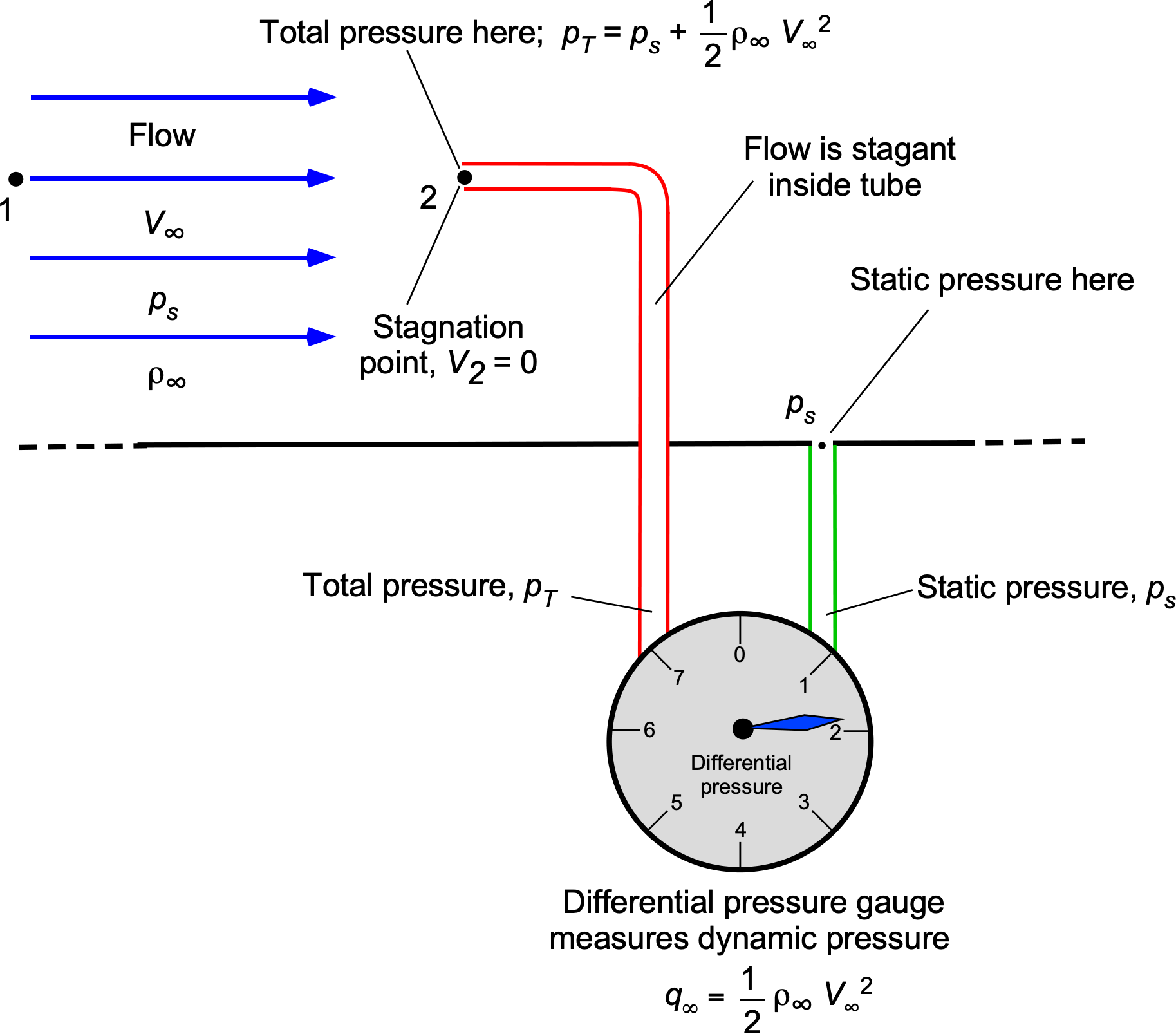
But at point 2 at the entrance to the Pitot tube, the fluid is brought to rest, so $V_{2} = 0$ , i.e., it is a stagnation point, and

(12) $\begin{equation*} p_1 + \dfrac{1}{2} \, \varrho_{\infty} \, V_{1}^2 = p_{2} = \mbox{Total pressure at point 2} \end{equation*}$

The static pressure $p_1 = p_{s}$ must be measured to obtain the flow velocity from this latter expression. As in the Venturi problem, this static pressure can be measured with a separate static vent or with the ports on the outer side of a combined Pitot-static tube. Solving for $V_{1}$ gives

(13) $\begin{equation*} V_{1} = V_{\infty} = \sqrt{\frac{ 2\left(p_{2} - p_{s}\right)}{\varrho_{\infty}}} \end{equation*}$

Therefore, the freestream flow velocity, ${V_{\infty}}$ , can be measured by measuring the difference between a flow’s total and static pressure.

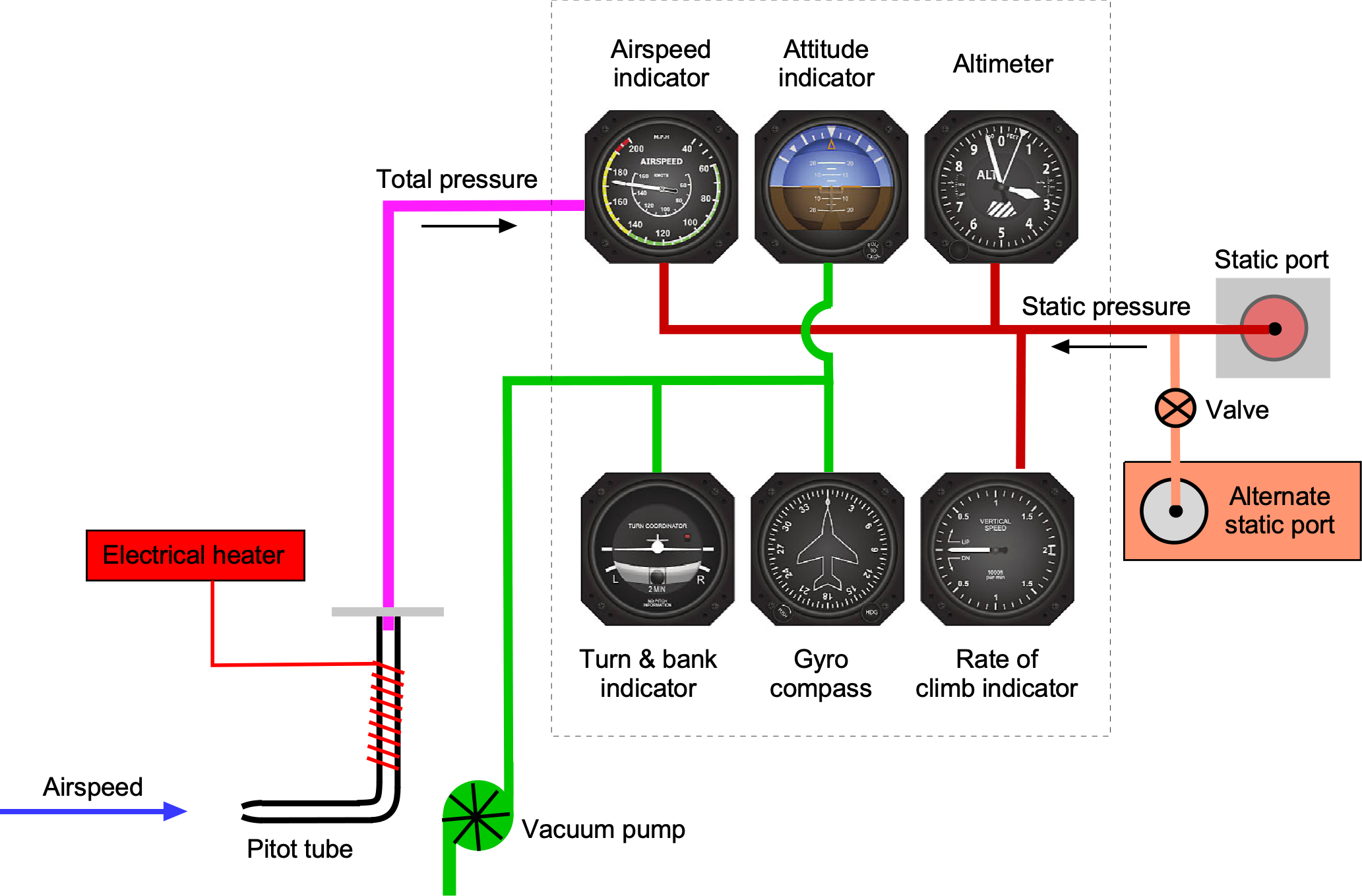
While a pitot-static probe is sometimes used to measure dynamic pressure, it is generally more accurate to measure dynamic pressure with a separate pitot probe and static vent, as shown in Figure 4. On an airplane, the static vent or source is usually located somewhere on the side of the fuselage. There may also be multiple static vents for redundancy. Pitot probes are mounted in the flow, away from the aircraft’s surface; they may be mounted on the nose or, in some cases, under the wing. The total pressure is connected to the airspeed indicator (ASI), with the static pressure being connected to the altimeter and vertical speed indicator. A heating element is used on the Pitot probe to prevent icing and avoid false ASI readings.

A typical pitot-static system on an airplane provides the reference pressures needed for the airspeed indicator and other pneumatic instruments. In this case, a pitot probe measures total pressure, and a separate static vent measures the static reference pressure.

Measuring Total Pressure

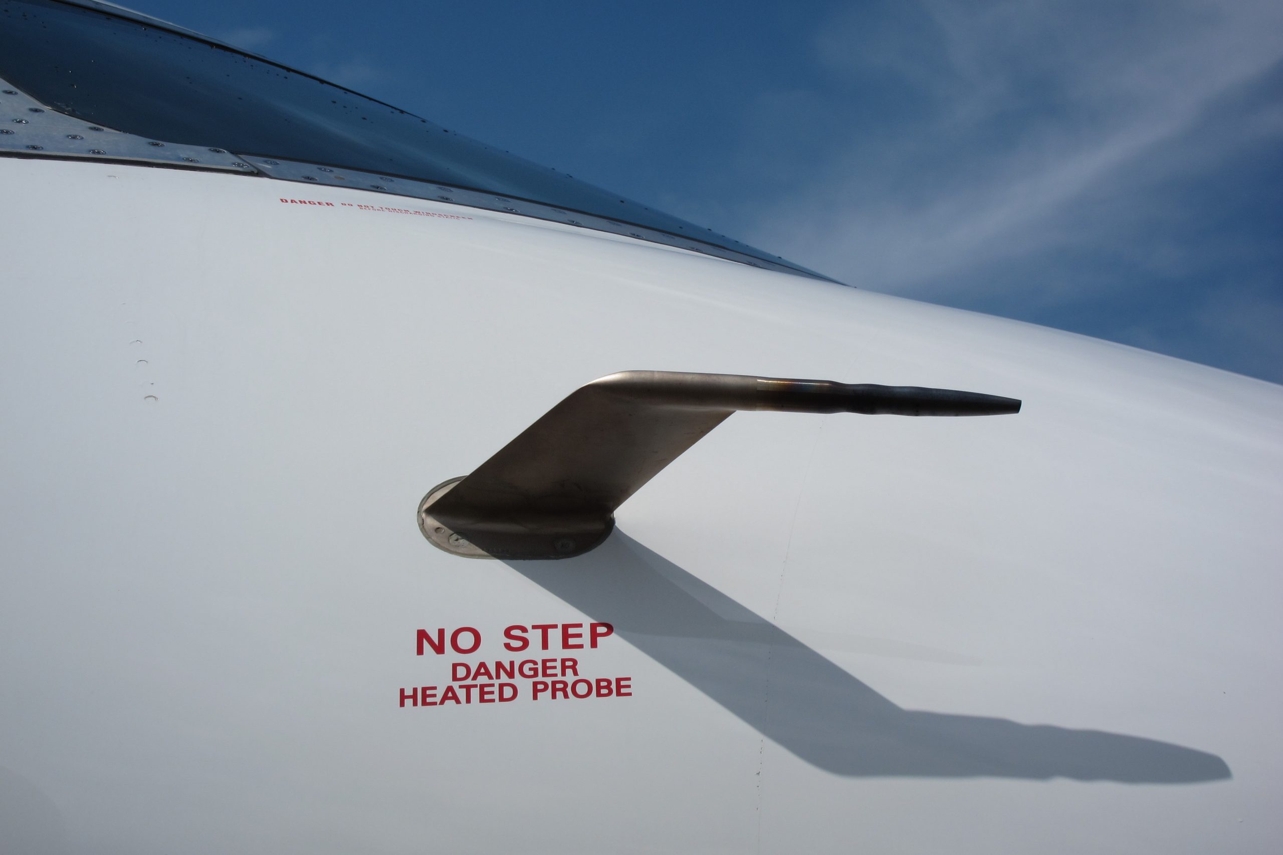
The total (ram) pressure can be measured with little error because the probe points directly into the airflow, and the resulting pressure is relatively high compared with the static pressure. The inlet shape of the Pitot tube must be clean and smooth to prevent pressure losses or other pressure disturbances that could affect the reading. The photograph in Figure 5 shows a total-pressure probe mounted on an aircraft’s nose. The probe must be well outside the surface boundary layer, displaced a short distance from the aircraft’s skin. Such probes must not be located where they could be subject to upstream flow disturbances, such as those caused by propellers, antennas, air scoops, or other probes.

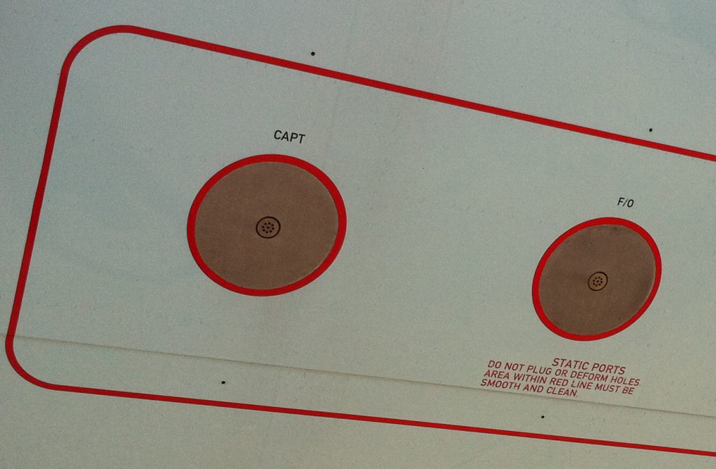
A Pitot probe is mounted on the right side of the nose of an airplane.

Measuring Static Pressure

Static pressure is often more challenging to measure accurately because of its relatively low value. It is measured on the airplane’s outer skin, as shown in Figure 6, usually at a location where the local static pressure is close to the ambient static pressure. However, there is no point on the surface at which the local static pressure exactly equals the static pressure in the freestream. Therefore, the static pressure measurement available to the ASI is always in error to some degree, a condition known as the static position error (SPE).

Static vents on the side of the nose of an airplane. Notice the multiple, separate vents for redundancy in case one or more become blocked.

Static Position Error (SPE)

The “error-free” issue in airspeed measurement mentioned previously requires further elaboration because the preceding arguments are predicated on two major points:

Both the total and static pressures can be measured accurately.
The ASI can be adequately calibrated against a suitable reference in terms of speed units.

One source of error is the Static Position Error (SPE), which is the difference between the measured local static pressure outside the aircraft and the actual static pressure at that altitude and airspeed. If the IAS reading is corrected for the SPE and mechanical errors, the resulting speed is called the calibrated airspeed (CAS). If the SPE and mechanical instrument errors are small, it is sufficient to state that IAS = CAS ≈ EAS. However, it is essential to note that, in general, the IAS differs from the EAS and the TAS.

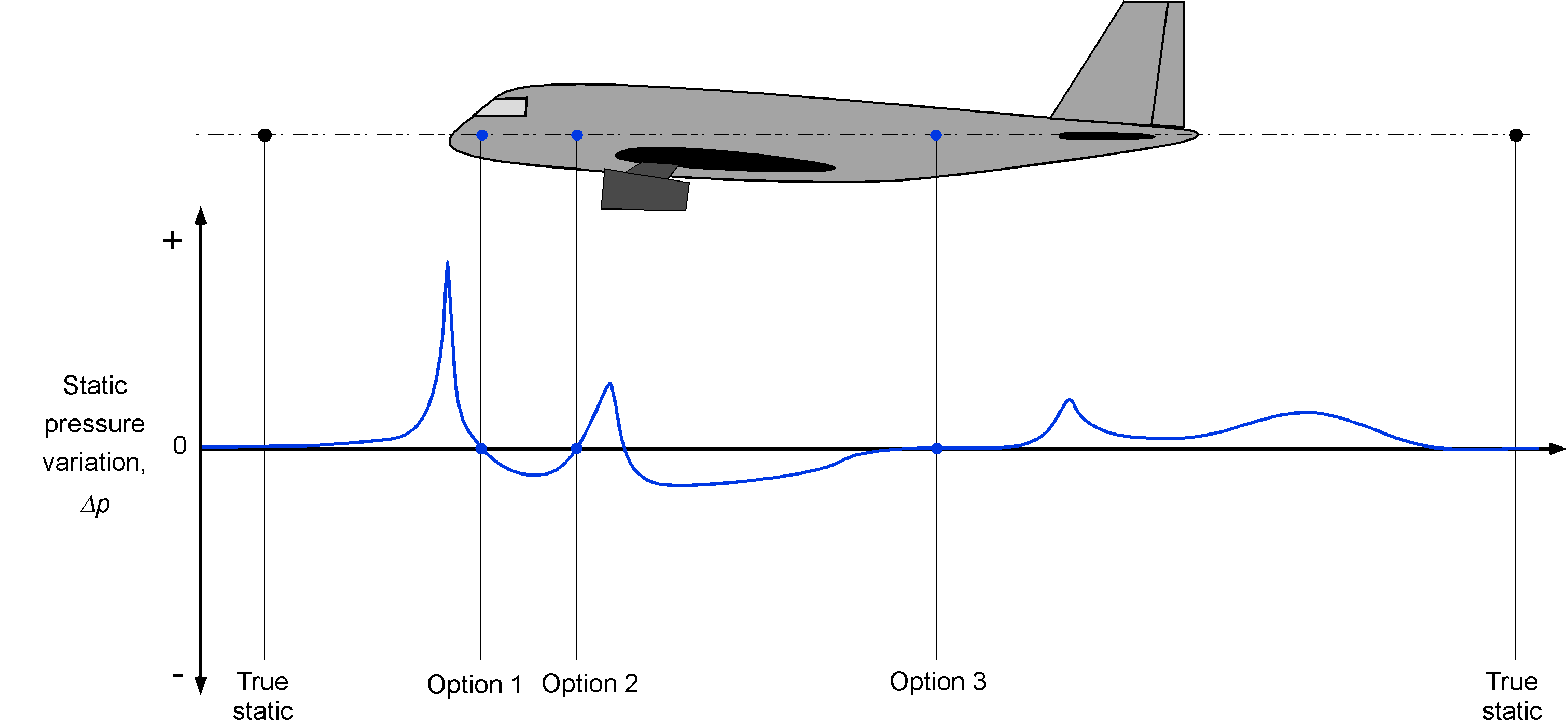
The effects of SPE must be measured and, in most cases, corrected for use in engineering and piloting. This process uses a formal calibration during flight testing with the specific make and model of the aircraft. The actual static pressure measurements are compared with the local static pressure measured at the pressure tap(s) on the aircraft’s outside skin. As shown in Figure 7, there are a few points on the outside skin of the aircraft where the local static pressure equals the true static pressure at which the aircraft is flying. The static pressure port on a prototype aircraft is typically repositioned after flight tests to minimize SPE, ultimately locating it at the SPE minimum. This location is then used on production versions of the aircraft. However, the SPE will never be precisely zero.

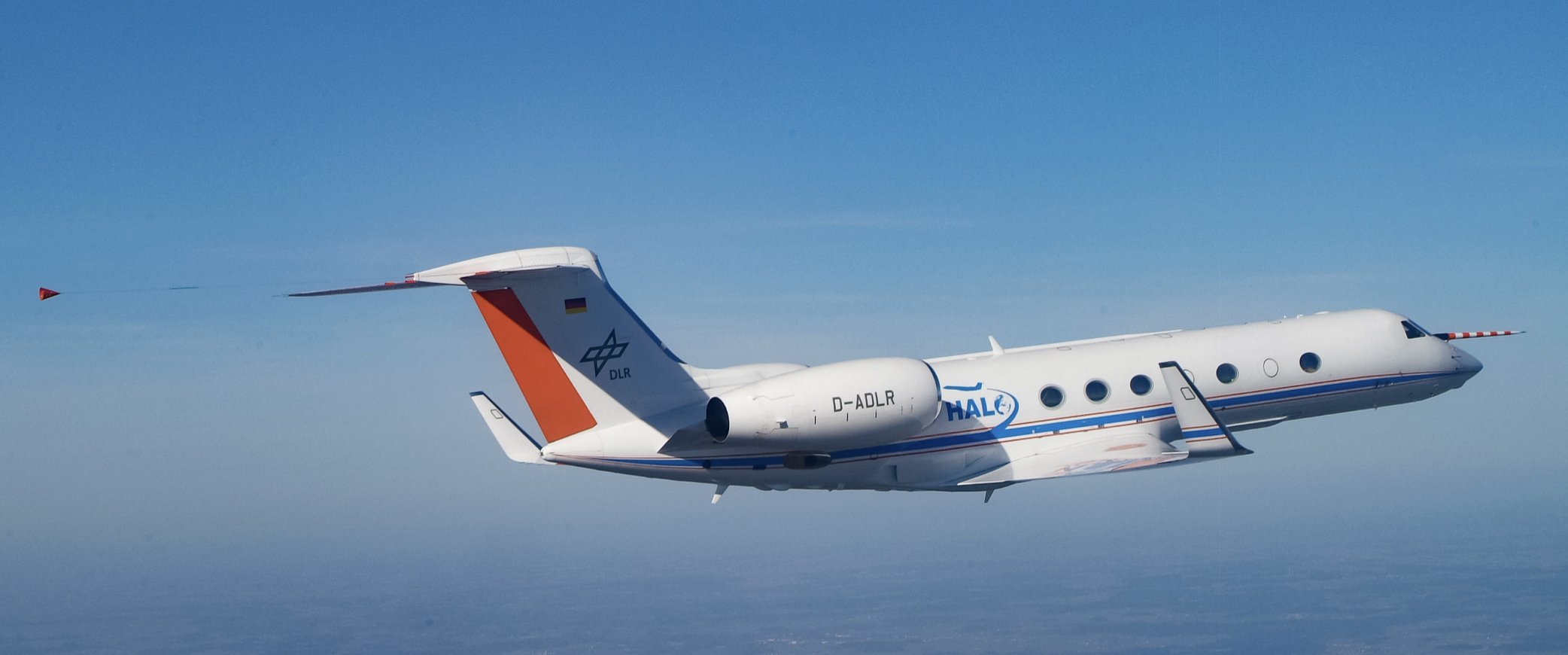
Several options exist for placing a static pressure port to minimize the SPE, although it will vary somewhat with airspeed and altitude.

During flight testing, the SPE calibration process measures the actual (true) static pressure at a location well aft of the aircraft using a trailing-cone apparatus, as shown in the schematic of Figure 8. Switching between the static pressure measured on the airplane and that measured by the trailing cone enables the pressure difference $\Delta p$ to be determined, which is the SPE.

The trailing cone method is used to calibrate the pitot-static system on a test aircraft, accounting for static-position errors arising from the placement of the static pressure tap(s) on the airframe.

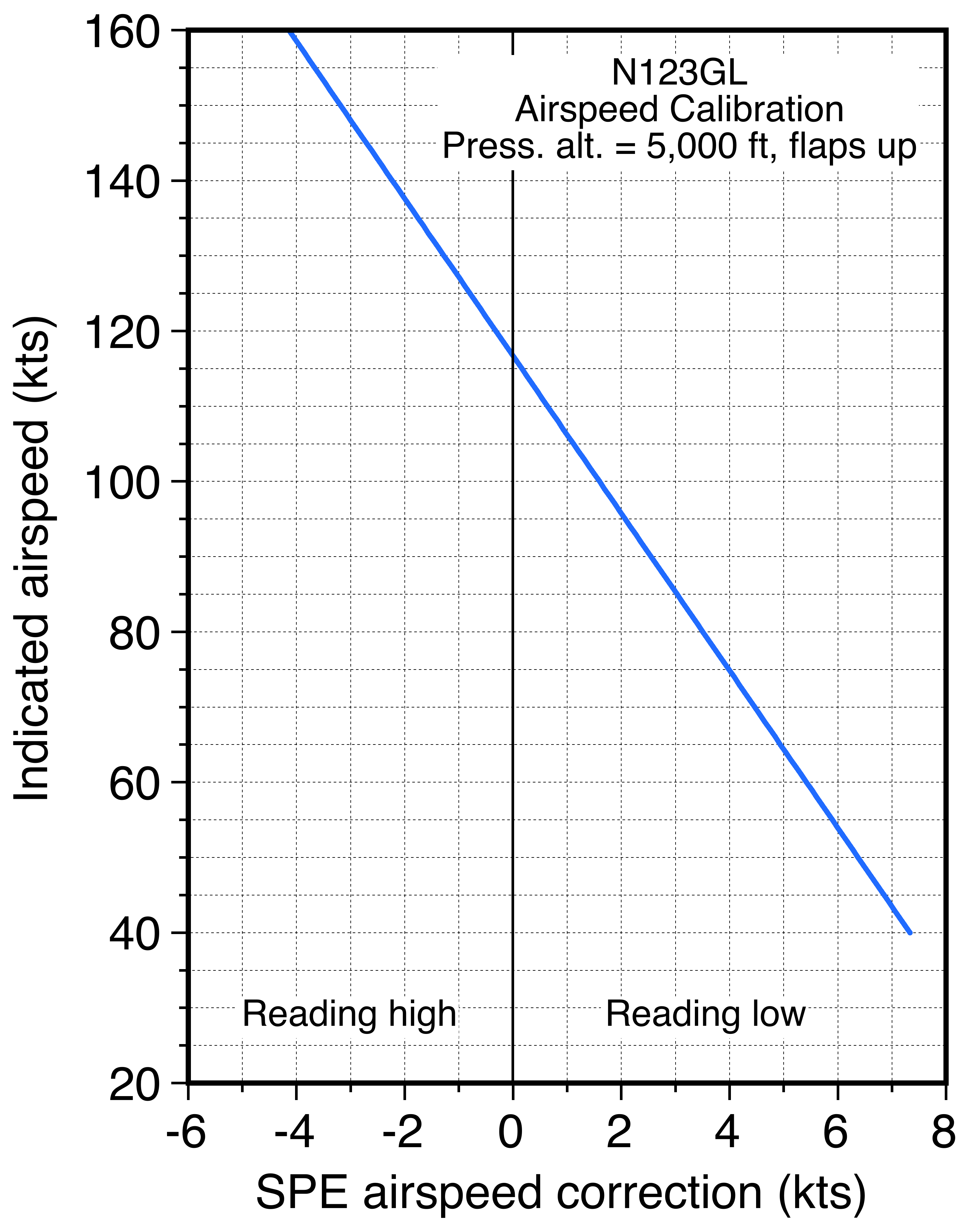
The photograph in Figure 9 illustrates a typical aircraft configuration during a calibration flight, with the trailing cone partially deployed. The cone is often trailed to several aircraft lengths to ensure undisturbed pressure measurements. The SPE varies slightly with airspeed and altitude, so it must be mapped across the aircraft’s entire operating envelope. Therefore, obtaining the necessary pressure data can require many hours of flight testing.

The trailing cone method being used on an airplane dedicated to flight testing.

The SPE is typically highest at low airspeeds, lower at high speeds, and higher at high altitudes, as shown in Figure 10. For higher-performance airplanes, such as jets, the SPE is likely a function of flight Mach number. The process must also be conducted with the aircraft in both the “clean” configuration (i.e., flaps and landing gear retracted) and the “dirty” configuration (i.e., flaps and landing gear extended, such as for landing).

An airspeed SPE correction chart. The indicated airspeed may read higher or lower than the equivalent airspeed.

The results obtained and the subsequent corrections derived as the SPE affects airspeed readings will apply to all production aircraft of the same make and model. The SPE results (or the corrected airspeed values), as required by FAA or EASA regulations, are always included in the aircraft’s flight manual. In the case of a modern airliner, the correction is incorporated into the EFIS via a software update to the airspeed indication. For piloting purposes, the SPE and mechanical errors are usually small enough to be ignored on many aircraft (perhaps a couple of kts). However, for engineering purposes, all such errors must be accurately accounted for in all aircraft performance analyses.

Mechanical Errors

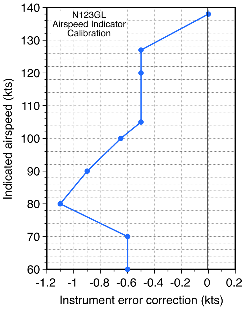
The mechanical error in the ASI can be determined in a laboratory setting by calibrating against a reference standard, resulting in a standard mechanical error calibration chart or table, as shown in the example in Figure 11. Each instrument error correction (IEC) calibration is specific to a particular ASI, and a different calibration is required if the ASI is replaced. The errors are usually small enough to be unimportant for piloting, but they should be included in any data-reduction process for engineering work.

A mechanical instrument error correction (IEC) chart for an ASI. The ASI may read high or low, depending on the specific ASI. Each ASI has its own IEC chart.

Check Your Understanding #1 – Correcting an ASI reading

A test aircraft is flying at a pressure altitude of 4,200 ft where the outside air temperature is 68.4 $^{\circ}$ F. The airspeed indicator (ASI) reads 134.5 kts. Calibrations available show the mechanical error of the ASI, $\Delta V_{E}$ , is -0.7 kts, and the static position error, $\Delta V_{\rm SPE}$ , is equivalent to +0.3 knots. Calculate the true airspeed of the aircraft.

Show solution/hide solution.

The ISA ambient temperature at this pressure altitude is

$T = T_0 - B \, h = 59 - 0.00357 \times 4,200 = 44.0~\mbox{$^{\circ}$F}$

The actual air temperature is warmer than ISA by

$68.4 - 44.0 = 24.4~\mbox{$^{\circ}$F}$

First, the indicated airspeed must be corrected for instrument and position errors to obtain the calibrated airspeed, so

$V_{\rm CAS} = V_{\rm IAS} - \Delta V_E - \Delta V_{\rm SPE}$

Hence,

$V_{\rm CAS} = 134.5 - (-0.7) - 0.3 = 134.9~\mbox{kts}$

At this relatively low speed, compressibility effects are negligible, so

$V_{\rm EAS} \approx V_{\rm CAS} = 134.9~\mbox{kts}$

Using the ISA pressure at 4,200 ft together with the measured outside air temperature gives an air density of approximately $\varrho_{\infty} = 0.00200~\mbox{slug/ft}^3$ , so that

$\sigma = \frac{\varrho}{\varrho_0} = \frac{0.00200}{0.002378} = 0.841$

Therefore, the true airspeed of the aircraft is then

$V_{\rm TAS} = \frac{V_{\rm EAS}}{\sqrt{\sigma}} = \frac{134.9}{\sqrt{0.841}} = 147.1~\mbox{kts}$

Airspeed Measurement at Higher Mach Numbers

The issue of airspeed measurement at higher speeds, where compressibility effects become significant, must also be addressed. In this case, the Bernoulli equation is not applicable. In practice, compressibility effects on airspeed measurement are negligible below approximately 10,000 feet and 200 knots. At higher altitudes, the lower air temperatures decrease the speed of sound, thereby increasing Mach numbers, so that compressibility thresholds are met at lower airspeeds.

Remember that airspeed values on the ASI are referenced to MSL density conditions by calibrating the speed scale based on the assumption that $\varrho_{\infty} = \varrho_0$ , so the corresponding equivalent airspeed or EAS is then

(14) $\begin{equation*} V_{\rm {\tiny EAS}} = \sqrt{ \frac{p^* - p_s }{2 \, \varrho_0} } = \sqrt{ \frac{\Delta p}{2 \, \varrho_0}} \end{equation*}$

The ASI continues to function as a dynamic pressure-measuring instrument. However, the compressibility of air affects the measurement of total pressure using a Pitot tube, so this must be accounted for.

Subsonic Flight Speeds

For subsonic Mach numbers above about $M_\infty \gtrsim 0.3$ , compressibility effects become significant, and the relationship between the total pressure, $p^*$ , and the static pressure, $p_s$ , must be obtained from the isentropic flow relations. In this case

(15) $\begin{equation*} \frac{p^*}{p_s} = \left( 1+\frac{\gamma-1}{2}M_\infty^2 \right)^{\gamma/(\gamma-1)} \end{equation*}$

This expression can be inverted to determine the Mach number directly from the measured pressure ratio, i.e.,

(16) $\begin{equation*} M_\infty = \sqrt{ \frac{2}{\gamma-1} \left[ \left(\frac{p^*}{p_s}\right)^{(\gamma-1)/\gamma} -1 \right] } \end{equation*}$

Therefore, the Pitot-static system provides a direct measurement of the flight Mach number when compressibility effects are accounted for.

In higher-speed subsonic flight, it is also necessary to measure the total (stagnation) temperature, $T_T$ , from which the speed of sound and the true airspeed can be determined. The speed of sound based on the total temperature is

(17) $\begin{equation*} a_T = \sqrt{\gamma \, R \, T_T} \end{equation*}$

Because the total and static temperatures are related by

(18) $\begin{equation*} T_T = T \left( 1+\frac{\gamma-1}{2}M_\infty^2 \right) \end{equation*}$

the static speed of sound, $a = \sqrt{\gamma R T}$ , can be written as

(19) $\begin{equation*} a = \frac{a_T} {\sqrt{1+\dfrac{\gamma-1}{2}M_\infty^2}} \end{equation*}$

Therefore, the true airspeed (TAS) becomes

(20) $\begin{equation*} V_{\rm {\tiny TAS}} = a\,M_\infty = \frac{a_T\,M_\infty} {\sqrt{1+\dfrac{\gamma-1}{2}M_\infty^2}} \end{equation*}$

Once the Mach number and atmospheric conditions are known, both the equivalent airspeed (EAS) and the true airspeed (TAS) can be determined consistently.

Check Your Understanding #2 – Finding the flight Mach number & TAS

An experimental turboprop airplane is flying at a pressure altitude of 25,000 ft. The Pitot-static system monitored by the test engineers measures the total pressure, $p^*$ , as 30.65 kPa, and the corrected static pressure, $p_s$ , as 23.91 kPa. What are the aircraft’s flight Mach number and true airspeed (TAS)? Assume: 1. ISA standard conditions. 2. No mechanical or SPE errors.

Show solution/hide solution.

Using the compressible-flow relation,

$\frac{p^*}{p_s} = \left( 1 + \frac{\gamma - 1}{2} M_{\infty}^2 \right)^{\gamma/(\gamma -1)}$

For air, $\gamma = 1.4$ , so

$\frac{30{,}650}{23{,}910} = 1.282 = \left( 1 + 0.2 \, M_{\infty}^2 \right)^{3.5}$

and so

$M_{\infty} = \sqrt{\frac{1.282^{0.2857}-1}{0.2}} = 0.606$

At a pressure altitude of 25,000 ft under ISA conditions, the speed of sound is $a = 1016.0~\mbox{ft/s}$ . Therefore, the true airspeed is

$V_{\rm TAS}=a \, M_{\infty}= 1,016.0 \times 0.606 = 616.0~\mbox{ft/s} \approx 365~\mbox{kts}$

Note: Determining the actual speed of sound, other than for assumed ISA conditions, requires measuring the outside air temperature.

Supersonic Flight Speeds

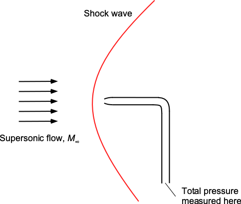
At supersonic Mach numbers, a bow shock forms ahead of the Pitot probe (Fig. 12), so the flow does not decelerate isentropically. Instead, the flow first passes through a normal shock and then decelerates isentropically to the stagnation point. The probe therefore measures the total pressure behind the shock, $p_{0_2}$ .

A Pitot tube in a supersonic flow produces a shock wave ahead of the tube, requiring shock-wave relations to determine the total pressure.

Let the freestream conditions be denoted by subscript 1 and the post-shock conditions by subscript 2. Across the normal shock,

(21) $\begin{equation*} \frac{p_2}{p_1} = \frac{2 \, \gamma \, M_\infty^2 - (\gamma-1)}{\gamma+1} \end{equation*}$

and the downstream Mach number is

(22) $\begin{equation*} M_2^2 = \frac{1+\dfrac{\gamma-1}{2}M_\infty^2} {\gamma M_\infty^2 - \dfrac{\gamma-1}{2}} \end{equation*}$

The flow then decelerates isentropically to give

(23) $\begin{equation*} \frac{p_{0_2}}{p_2} = \left( 1+\frac{\gamma-1}{2}M_2^2 \right)^{\gamma/(\gamma-1)} \end{equation*}$

Combining these relations yields the Rayleigh–Pitot tube formula

(24) $\begin{equation*} \frac{p_{0_2}}{p_1} = M_\infty^2 \left(\frac{\gamma+1}{2}\right) \left[ \frac{(\gamma+1)^2 M_\infty^2} {4 \,\gamma \, M_\infty^2 - 2(\gamma-1)} \right]^{1/(\gamma-1)} \end{equation*}$

Because $M_\infty$ appears implicitly, it must be obtained iteratively from the measured pressure ratio.

Summary of Airspeed Definitions

The following airspeed definitions are commonly used in aviation:

1. TAS is the true airspeed, which is the actual speed of the aircraft relative to the surrounding air mass. In engineering analyses, this is written as ${V_{\infty}}$ .

2. IAS is the indicated airspeed, which is the speed displayed directly by the airspeed indicator (ASI). It is based on the measured dynamic pressure, assuming standard sea-level density, i.e., $\varrho_{\infty} = \varrho_0$ , and includes both instrument and position errors.

3. CAS is the calibrated airspeed, which is the indicated airspeed corrected for instrument (mechanical) errors and static position error (SPE). It represents the airspeed corresponding to the measured dynamic pressure in the absence of these errors.

4. EAS is the equivalent airspeed, which is the airspeed corresponding to the same dynamic pressure at sea-level density, i.e., $q = \tfrac{1}{2} \, \varrho_0 \, V_{\rm {\tiny EAS}}^2$ . It is obtained from CAS by correcting for compressibility effects, which become significant for $M_\infty \gtrsim 0.3$ . The true airspeed is then obtained from the equivalent airspeed using the density ratio, i.e.,

$V_{\rm {\tiny TAS}} = \frac{V_{\rm {\tiny EAS}}}{\sqrt{\sigma}} = V_{\rm {\tiny EAS}}\sqrt{\frac{\varrho_0}{\varrho}} \, , \quad \text{where} \ \sigma = \varrho/\varrho_0$

Optical Airspeed Measurements

Laser Doppler Velocimetry (LDV) offers a non-intrusive optical method for measuring true airspeed during flight, particularly in conditions where traditional Pitot-static pneumatic systems lose accuracy. Such conditions include flight at low airspeeds and low dynamic pressures, or any conditions around the aircraft that cause significant static position error (SPE). This LDV device is beneficial for airspeed measurement during low-speed phases of flight, particularly in helicopters and other rotorcraft, such as eVTOLs, where the SPE remains large below approximately 50 kts. In principle, LDV systems can provide free-air measurements at any airspeed, from near-zero or negative to subsonic, supersonic, and hypersonic speeds.

A typical LDV airspeed setup consists of a laser source, beam-splitting optics, and a focusing lens mounted externally on the aircraft, as illustrated in Figure 13. The lens has a relatively long focal length to direct two coherent laser beams so they intersect at a fixed point in the undisturbed freestream flow well ahead of the aircraft. The intersection of the laser beams forms a small ellipsoidal measurement volume with a major axis typically on the order of 0.1 mm, resulting in an interference fringe pattern.

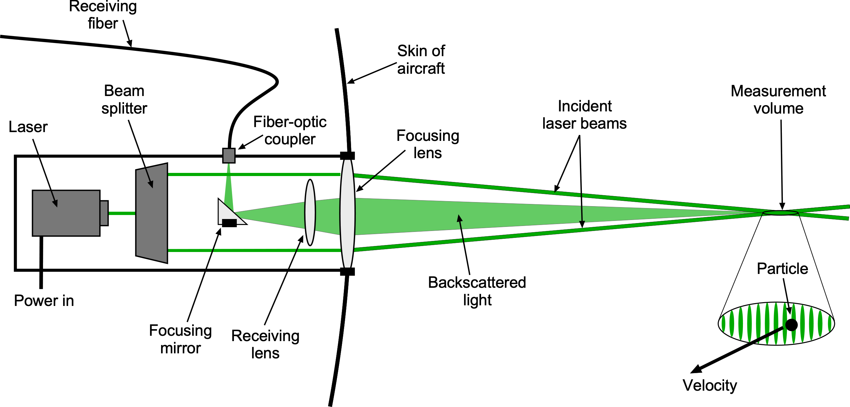
A typical LDV airspeed setup includes a laser source, beam-splitting optics, and a focusing probe mounted externally on the aircraft.

As naturally occurring particles in the atmosphere pass through this fringe pattern, they scatter Doppler-shifted light or “Doppler bursts” based on their velocity. This scattered light is collected and focused onto the end of a fiber-optic cable, which is then connected to a photodetector and then to a signal conditioner. The Doppler frequency is then extracted electronically to determine the instantaneous particle velocity corresponding to the aircraft’s airspeed. Because many bursts arrive in rapid succession, real-time averaging can be used to compute the instantaneous airspeed, that is, its actual speed relative to the surrounding air.

The natural atmosphere typically contains sufficient aerosol-sized particles to scatter light effectively within the measurement volume. Volcanic eruptions, in particular, release significant quantities of fine particulate matter, usually in the micron diameter range, into the upper troposphere and lower stratosphere. These particles can remain suspended over large regions of the Earth’s atmosphere for extended periods, providing ample seeding for in-flight LDV measurements.

The primary advantage of LDV is its independence of SPE, compressibility effects, and boundary-layer distortions, all of which can affect the performance of Pitot tubes and static pressure ports. To ensure accurate airspeed measurements, the LDV probe must be calibrated and aligned with the aircraft’s body axes. Misalignment can introduce biases and errors in the measured airspeed. Some systems incorporate inertial measurement units (IMUs) or GPS to provide reference velocity data and to correct for platform motion. In more advanced configurations, differential LDV systems using multiple laser wavelengths are employed to measure airspeed along with the other two components of the aircraft’s velocity vector.

LDV-based airspeed measurement systems have been successfully demonstrated in flight research programs for fixed-wing aircraft and rotorcraft. Pneumatic calibration systems use wingtip booms, nose-mounted probes, or trailing-cone systems to provide reference airspeed measurements outside disturbed-flow regions. LDV-based airspeed measurement systems focus the laser beam into a measurement volume well upstream of the aircraft, ensuring that measurements are taken in undisturbed air. However, errors arising from optical misalignment, beam-quality degradation, aircraft vibrations, and aeroelastic deformations can degrade signal quality. However, such issues can be mitigated with ruggedized fiber-coupled optics, vibration-isolated mounts, and adaptive signal filtering techniques.

Despite its relative complexity compared to conventional pneumatic systems, LDV is currently one of the most precise methods for measuring airspeed. With continued advances in compact and rugged optical hardware, LDV-based airspeed measurement systems will likely see wider adoption, especially for rotorcraft. Companies such as Optical Air Data Systems are at the forefront of this technology. While such systems may never completely replace conventional pneumatic airspeed measurement systems, they will be an essential augmentation for low airspeed measurements across all aircraft types.

Summary & Closure

Airspeed measurement is straightforward using a pitot-static system; however, it is essential to understand precisely which airspeed is being measured, i.e., equivalent airspeed, calibrated airspeed, or true airspeed. Engineers usually require a measurement of the aircraft’s true airspeed, which must be obtained indirectly through calculations. True airspeed is not a direct measurement. Pilots, however, require both the equivalent airspeed (to which the aircraft responds aerodynamically) and the true airspeed (for navigation purposes). Static position errors and mechanical errors in airspeed measurement must also be addressed.

One must also remember that the ASI is calibrated using mean sea-level (MSL) density, i.e., assuming that $\varrho_{\infty} = \varrho_0$ . At higher subsonic and supersonic airspeeds, compressibility effects affect the measurement of total and static pressures using a Pitot probe, necessitating appropriate corrections (based on isentropic flow relations) to determine the Mach number and true airspeed. At supersonic airspeeds, additional issues arise, including the need to relate total and static pressure measurements to the flow across shock waves.

5-Question Self-Assessment Quickquiz

For Further Thought or Discussion

An airplane is flying at a pressure altitude of 10,000 ft with an indicated airspeed of 200 kts. What is its true airspeed? Hint: Assume no SPE and an error-free airspeed indicator.
In practical aviation, why does a pilot need the indicated airspeed and the ground speed?
What might be the consequences if an aircraft is found to have a significant static position error? For the pilot? For engineering analysis?
Research the effects of compressibility on airspeed measurement. What happens to the reading from a pitot probe when an aircraft exceeds the speed of sound?
Can you explain the concept of airspeed limitations and how they are indicated on the instrument?
What are the limitations of airspeed indicators and the factors that can affect their accuracy?
Can you describe the effects of airspeed on aircraft performance?
How are airspeed indicators calibrated and tested for accuracy?
Air France 447 Accident: Explain how a failed Pitot tube resulted in the loss of control of the aircraft.

Other Useful Online Resources

Great video on “The Airspeed Indicator & Types of Airspeed.”
This video explains how a barometric altimeter works and how the readings are interpreted.
To learn more about the evolution of aircraft instruments, read “70 Years of Flight Instruments and Displays.”
An excellent discussion on air data measurement and calibration by NASA.

License

Icon for the Creative Commons Attribution-NonCommercial-NoDerivatives 4.0 International License

Introduction to Aerospace Flight Vehicles Copyright © 2022–2026 by J. Gordon Leishman is licensed under a Creative Commons Attribution-NonCommercial-NoDerivatives 4.0 International License, except where otherwise noted.

Digital Object Identifier (DOI)

https://doi.org/https://doi.org/10.15394/eaglepub.2022.1066.n29