Dynamic Similarity

J. Gordon Leishman

doi:https://doi.org/10.15394/eaglepub.2022.1066.n14

17 Dynamic Similarity

Introduction

The principle of dynamic similarity is closely connected to the concepts used in dimensional analysis. The need for similarity or similitude is a concept that always arises when testing sub-scale engineering models in the laboratory or the wind tunnel. A sub-scale model application is said to have similitude with the actual (real) application if the two applications share the same geometric, kinematic, and dynamic similarities. In general, geometric similarity focuses on the scaling of dimensions, kinematic similarity on the scaling of displacements and velocities, and dynamic similarity on the scaling of integrated values such as forces. A prerequisite for dynamic similarity is geometric similarity and kinematic similarity. Therefore, any claim that “dynamic similarity” has been achieved implies that geometric and kinematic similarity conditions have also been met.

Dynamic similarity can be achieved by matching the values of the similarity parameters between two different circumstances, e.g., in two or more separate experiments or at model scale and full scale, which may be challenging to achieve in practice. If the values of the similarity parameters are the same, then the physics of both situations will be correctly scaled, so both will have the correct physical similarity. As previously discussed, the critical aerodynamic similarity parameters are the Reynolds and Mach numbers. However, in general, many other relevant similarity parameters arise in aerodynamics and engineering problem-solving, such as the Froude number, Weber number, Strouhal number, Stokes number, Prandtl number, Womersley number, etc. Similarity parameters of various types are used in all fields of engineering. Therefore, understanding the principles associated with dynamic similarity and applying them is very important in engineering analyses.

Learning Objectives

Understand the concepts of geometric, kinematic, and dynamic similarity and appreciate their significance as another tool for engineering problem-solving.
Use dimensional analysis to understand how problem parameters scale to achieve dynamic similarity, i.e., how the problem scales with geometrical size, operating conditions, etc.
Appreciate the challenges of using scaled models in the laboratory and wind tunnel testing to obtain measurements that can be applied to full-scale flight vehicles.
Realize the benefits and limitations of testing actual (full-scale) problems on a smaller scale and why only partial similarity may be possible in some cases.

Similarity Criteria

The following formal criteria are required to achieve flow similarity or similitude between the model or sub-scale test article and the eventual or actual application:

Geometric similarity means the sub-scale model is scaled correctly and has the same geometrical shape as the actual application. Thus, a single scaling parameter can relate the two geometries.
Kinematic similarity means that the displacements and velocities of the sub-scale model and the actual application must be the same.
Dynamic similarity means that the ratios of all forces and moments in the sub-scale model and the actual application are the same, i.e., inertial, gravitational, viscous, pressure, elastic, surface, etc. If dynamic similarity is obtained, geometric and kinematic similitude conditions will also be met.

Suppose all relevant similarity parameters for a given problem can be matched. In this case, it can be ensured that the physics of both situations are correctly scaled and have the correct physical similarity. Therefore, engineers can usually study the physical characteristics of the full or larger-scale system (e.g., one still in the design process) at a smaller scale and under the controlled environment of the laboratory or in the wind tunnel. Unfortunately, matching all relevant similarity parameters at a smaller scale is difficult, so only partial similarity may be possible. In that case, there are still techniques that can be used to obtain the desired results that will apply to the full-scale application.

Navier-Stokes Equations

The scaling significance of the Reynolds number and the Mach number can also be determined from the momentum equation of fluid motion, which is called the Navier-Stokes equation. The incompressible form of the Navier–Stokes equation can be written as

(1) $\begin{equation*} \varrho \frac{D\vec{V}}{Dt} = -\nabla p + \mu \nabla^2 \vec{V} \end{equation*}$

which is a vector equation. The Navier-Stokes equation is one of the most fundamental governing equations of fluid dynamics. Dividing Eq. 1 through by $\varrho$ gives

(2) $\begin{equation*} \frac{D\vec{V}}{Dt} = -\frac{1}{\varrho}\nabla p + \frac{\mu}{\varrho}\nabla^2 \vec{V} \end{equation*}$

If the velocities are scaled by a reference speed $V_\infty$ , i.e., defining the nondimensional velocity as

(3) $\begin{equation*} \vec{U}=\frac{\vec{V}}{V_\infty} \end{equation*}$

and lengths by a characteristic dimension $L$ , the nondimensional form of the Navier-Stokes equation becomes

(4) $\begin{equation*} \frac{D\vec{U}}{Dt} = -\nabla p + \frac{\mu}{\varrho V_\infty L}\nabla^2 \vec{U} = -\nabla p + \frac{1}{Re}\nabla^2 \vec{U} \end{equation*}$

where the Reynolds number is $Re = \dfrac{\varrho V_\infty L}{\mu}$ .

For compressible flows, an additional parameter appears, namely the Mach number, given by

(5) $\begin{equation*} M = \frac{V_\infty}{a} \end{equation*}$

with $a$ being the speed of sound. When pressure is scaled by a dynamic pressure, e.g., $\dfrac{1}{2} \varrho_\infty V_\infty^2$ , the nondimensional form of the momentum equation takes the form

(6) $\begin{equation*} \frac{D\vec{U}}{Dt} = -\frac{1}{\gamma M^2}\nabla p + \frac{1}{Re}\nabla^2 \vec{U} \end{equation*}$

where ${\gamma}$ is the ratio of specific heats, i.e., $C_p/C_{\cal{V}}$ .

This nondimensionalization of the governing momentum equation reveals two essential properties:

Dynamic Similarity: Flows about geometrically similar shapes that share the same $Re$ and $M$ will exhibit identical behavior, regardless of the absolute scales of $V_\infty$ and $L$ .
Flow Regime Effects: The Reynolds number quantifies the ratio of inertial to viscous force. A higher $Re$ indicates that inertial effects are more important, reducing the relative influence of viscosity. The Mach number is a measure of compressibility effects. At a low $M$ ( $M \ll 1$ ) the flow is nearly incompressible, whereas for $M \ge 1$ , compressibility effects and shock waves become significant.

Aerodynamic Similarity

Using an aerodynamic example of flow similarity, consider two bodies to be tested in two wind tunnels to determine their relative aerodynamic performance. The bodies are said to be geometrically similar if the geometry of one body can be obtained by applying a single scale factor to the geometry of the other body, as shown in the figure below. However, suppose the two bodies (e.g., model versus the full-scale application) are not geometrically similar. In that case, kinematic and dynamic flow similarity can never be obtained, which is the end of the matter. Therefore, the need for geometrical similarity of the two bodies is a prerequisite to obtaining kinematic and dynamic flow similarity, hence the idea of correctly geometrically scaled models for use in the wind tunnel.

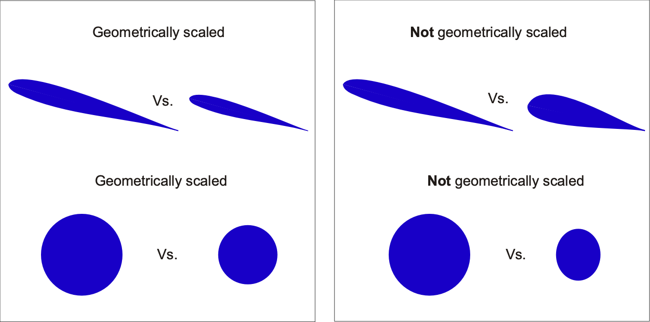
A prerequisite for flow similarity between two bodies is that their geometries are scaled by a single scaling factor.

Suppose all similarity parameters applicable to each geometrically scaled body can be made equal, e.g., the same values of the Reynolds number and the Mach number. In that case, the flows about each body will be kinematically and dynamically similar, and the results obtained at the model scale will apply to the full-scale application. Therefore, in summary, it can be stated that the flows about two bodies will be dynamically similar if:

The body shapes are geometrically similar, i.e., a single scaling factor relates the model and full-scale shapes.
All similarity parameters have the same values, such as Reynolds number $Re$ , Mach number $M$ , and other relevant similarity parameters.

In the case of aerodynamic problems, if it can be formally established that the flow similarity parameters have the same values for both flows at both scales and that the flows are dynamically similar, then:

The streamline patterns of both bodies will be geometrically similar. This means the flow patterns around both bodies will be the same.
The flow distributions of non-dimensional velocity, pressure coefficient, etc., will be the same when plotted against a standard non-dimensional length coordinate, i.e., a length scale non-dimensionalized by a characteristic length such as a chord.
The force coefficients (e.g., lift and drag coefficients) and moment coefficients (about the same non-dimensional reference point) will be the same.

The similarity parameters, Mach number and Reynolds number, are the most significant similarity parameters used in aerodynamics. Remember that the Reynolds number is always based on some characteristic length (e.g., chord, mean chord, diameter, etc.) and should be qualified as such. Other similarity parameters may be necessary for specific problems, especially when factors other than aerodynamic ones are involved. However, the effects of Mach number and Reynolds number inevitably come up in all aerospace flight vehicle problems in one form or another.

Wind Tunnel Testing

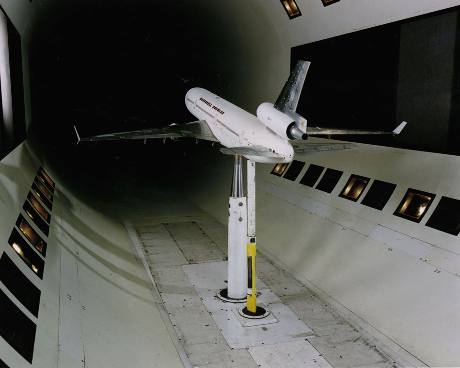
The concept of dynamic flow similarity is a fundamental issue in wind tunnel testing of sub-scale models. Suppose a sub-scale model of an actual (full-size) aircraft will be tested in a wind tunnel. In that case, the basic idea is to simulate the conditions of free flight, i.e., to simulate the actual flight conditions in the wind tunnel. In this case, the flow produced will give the same non-dimensional pressure distributions, as well as lift, moments, and drag coefficients, as on the actual aircraft during a free flight. However, this outcome can only be true if the Reynolds and Mach numbers attained in the wind tunnel test are the same as for free flight. Scaled models in a wind tunnel can help verify the aircraft design before tooling and construction begin, and in most cases, it is a critical step in the development process of a new aircraft.

Testing a sub-scale model in a wind tunnel. The model is an MD-11.

Unfortunately, it is difficult to obtain the proper scaling of both the Reynolds number and the Mach number in wind tunnel tests, mainly because the test article in the wind tunnel is usually a smaller (i.e., sub-scale) version of the actual aircraft. While the issues can be prevented using a wind tunnel big enough to test the full-scale flight vehicle, this is rarely practical. The biggest wind tunnel is the National Full-Scale Aerodynamics Testing Facility at NASA Ames Research Center, which has a test section 120 ft (36.6 m) wide and 80 ft (24.4 m) high. It can even accommodate actual aircraft with their engines running. However, it can only test at flow speeds up to about 120 knots. Therefore, most wind tunnel tests are performed with smaller or sub-scale models.

Challenges of Wind Tunnel Testing

During design, it is necessary to conduct wind tunnel tests on any new aircraft to verify predicted aerodynamic performance. For example, consider the design of a light aircraft. Assume that the full-scale aircraft is expected to cruise at a speed of 140 mph ( $V_{\infty}$ is approximately 50 ms $^{-1}$ ). The aircraft’s wingspan is 14 m, and the mean wing chord is 1.5 m.

For these preceding conditions, the Reynolds number based on the mean wing chord will be

(7) $\begin{equation*} Re = \frac{\varrho V_{\infty} c}{\mu} = \frac{1.23 \times 50 \times 1.5}{18.15 \times 10^{-6}} = 5.08 \times 10^6 \end{equation*}$

Similarly, the flight (free-stream) Mach number will be approximately

(8) $\begin{equation*} M = \frac{V_{\infty}}{a} = \frac{50}{330} = 0.16 \end{equation*}$

Therefore, this wing will operate in an essentially incompressible flow regime. The free-stream Mach number is so low (less than 0.3) that compressibility effects on the aerodynamics are likely negligible. Nevertheless, this does not prevent the need to match the Mach number as one of the required similarity parameters.

Suppose, for example, a scale model of this aircraft was to be tested in a wind tunnel with a 2.5-by-3.5 m working section (the region where the model is tested). Therefore, the wingspan of the model must be less than 3 m. Ideally, the wingspan should be between 50% and 70% of the maximum tunnel width, in this case, about 2 m. This size is essential to ensure that the wind tunnel walls do not disturb the flow over the wing; this is called a wind tunnel wall interference effect, and the effect should be minimized as much as possible.

A prerequisite for the dynamic flow similarity of the model is that the model must be geometrically similar to the actual aircraft. This requirement means something of the order of a 1/7-scale model would be needed, which can be manufactured by various means. Now, if the tunnel wind speed is set to 50 ms $^{-1}$ (which is the full-scale flight speed $V_{\infty}$ ), the Reynolds number based on the mean chord will be approximately

(9) $\begin{equation*} Re = \frac{\varrho V_{\infty} c}{\mu} = \frac{1.23 \times 50 \times 1.5/7}{18.15 \times 10^{-6}} = 0.72 \times 10^6 \end{equation*}$

So, it can be seen immediately that dynamic similarity cannot be obtained in this case because the Reynolds numbers between the wind tunnel test and full scale cannot be matched, even if the Mach number can be matched. This situation is called partial similarity.

What can be done here? Well, the wind speed could be increased. However, to get the required matching of the Reynolds numbers, the tunnel wind speed must be seven times 50 ms $^{-1}$ , which is 350 ms $^{-1}$ , and a wind speed of 350 ms $^{-1}$ will give a Mach number that is far too high (Mach 1.1!). So, even though the Reynolds numbers could be hypothetically matched, the Mach numbers would be incorrect. Therefore, one of the significant practical difficulties of wind tunnel testing of scale models is now apparent, at least using conventional wind tunnels.

One solution to this dilemma is changing the working fluid’s density or viscosity (or both). In this regard, hydrodynamic tests (in water) are sometimes performed on models because the kinematic viscosity of water is significantly less (about 1/15) than that of air. This means that smaller models tested at lower speeds in water can achieve almost the same Reynolds number as larger ones tested in faster-moving air. However, the issue of scaling the Mach number is also essential, bearing in mind that the ratio of the speed of sound in water compared to air is about 4:1. So, water as a test medium is not usually a good solution for simulating the parameters for flight vehicles.

Compressed air, helium, or a refrigerant gas type may allow higher Reynolds number testing of smaller models. For example, a pressurized wind tunnel could compress the air and increase its density. However, this is a complicated and expensive option because a special wind tunnel must be used. The density of the air could also be increased by cooling, which will, at the same time, decrease the viscosity. Air cooling could also be a viable option to increase the Reynolds number; unfortunately, the air must be cooled to very low temperatures to change its viscosity substantially. Therefore, it is necessary to use a cryogenic wind tunnel, which is very expensive to build and run.

The primary reason for using cryogenic temperatures is that they allow the attainment of higher Reynolds numbers. The Reynolds number can be written as

(10) $\begin{equation*} Re = \frac{\varrho \, V \, c}{\mu} = \left( \frac{\varrho \, a}{\mu} \right) M \, c \end{equation*}$

Therefore, for a given Mach number and model size, then

(11) $\begin{equation*} Re \, \propto \, \left( \frac{\varrho_{\infty} \, a_{\infty}}{\mu_{\infty}} \right) \end{equation*}$

For an ideal gas, then

(12) $\begin{equation*} \varrho_{\infty} \, \propto \, \frac{p_{\infty}}{T_{\infty}} \quad \mbox{and} \quad a_{\infty} \, \propto \, \sqrt{T_{\infty}} \quad \mbox{and} \quad \mu_{\infty} \, \propto \, \sqrt{T_{\infty}} \end{equation*}$

so that

(13) $\begin{equation*} Re \, \propto \, \left( \frac{p_{\infty}}{T_{\infty}} \right) \left( \frac{T_{\infty}^{1/2}}{T_{\infty}^{1/2}} \right) \approx \frac{p_{\infty}}{T_{\infty}} \end{equation*}$

Therefore, the Reynolds number increases with decreasing temperature for a given Mach number, model size, and tunnel operating pressure.

Helpful Scaling Laws

Many fluid parameters appear as ratios in similarity analysis, such as ratios of sound speeds, viscosity, density, etc. These ratios can frequently be reexpressed in terms of temperature ratios, which is quite helpful in establishing scaling factors and the relative values of similarity parameters, even if only approximately.

For example, the speed of sound is given by

(14) $\begin{equation*} a = \sqrt{ \gamma \, R \, T} \end{equation*}$

where $T$ is the absolute temperature. Therefore, in terms of the speed of sound ratio between two conditions, 1 and 2, then

(15) $\begin{equation*} \dfrac{a_1}{a_2} = \sqrt{ \frac{T_1}{T_2} } \end{equation*}$

The viscosity of a gas is approximately proportional to the square root of temperature, i.e., $\mu \, \propto \, \sqrt{T}$ , which is an outcome of the kinetic theory. Therefore, between the two conditions, 1 and 2, then

(16) $\begin{equation*} \dfrac{\mu_1}{\mu_2} \approx \sqrt{ \frac{T_1}{T_2} } \end{equation*}$

From thermodynamics, then $\varrho \, \propto \, 1/T$ at a constant pressure, so

(17) $\begin{equation*} \dfrac{\varrho_1}{\varrho_2} = \frac{T_2}{T_1} \end{equation*}$

Finally, the kinematic viscosity, $\nu (= \mu / \varrho) \, \propto \, T^{3/2}$ so that

(18) $\begin{equation*} \dfrac{\nu_1}{\nu_2}\approx \left( \frac{T_1}{T_2} \right)^{3/2} \end{equation*}$

While some of these preceding relationships are only approximate, they can be used to give reasonable estimates of the scaling effects that may exist from one condition to another and insight into how dynamic similarity may be obtained.

Check Your Understanding #1 – Confirming dynamic similarity

Consider two airfoils with the same profile shape and operating angle of attack but different chords and operating in two different fluids, as given in the table below. Determine whether or not the flows are dynamically similar.

$\small \mbox{\bf Airfoil 1}$

$\small \mbox{\bf Airfoil 2}$

$\small \alpha_1 = 5^{\circ}$

$\small\alpha_2 = 5^{\circ}$

$\small V_1 = 210~\mbox{ms}^{-1}$

$\small V_2 = 140~\mbox{ms}^{-1}$

$\small \varrho_1 = 1.2~\mbox{kg}^{-3}$

$\small \varrho_2 = 3.0~\mbox{kg}^{-3}$

$\small\mu_1 = 1.8 \times 10^{-5}~\mbox{kg m}^{-1}\mbox{ s}^{-1}$

$\small \mu_2 = 1.5 \times 10^{-5}~\mbox{kg m}^{-1}\mbox{s}^{-1}$

$\small a_1 = 300~\mbox{ms}^{-1}$

$\small a_2 = 200~\mbox{ms}^{-1}$

$\small c_1 = 1.0~\mbox{m}$

$\small c_2 = 0.5~\mbox{m}$

Show solution/hide solution.

The test for dynamic flow similarity requires the determination of the values of the similarity parameters, i.e., the Reynolds number and Mach number for each flow. For Airfoil 1, then for the Reynolds number

$Re_1 = \frac{\varrho_1 V_1 c_1}{\mu_1} = \frac{1.2 \times 210.0 \times 1.0}{1.8 \times 10^{-5}} = 1.4 \times 10^7$

and for the corresponding Mach number

$M_1 = \frac{V_1}{a_1} = \frac{210.0}{300.0} = 0.7$

For Airfoil 2, then for the Reynolds number

$Re_2 = \frac{\varrho_2 V_2 c_2}{\mu_2} = \frac{3.0 \times 140.0 \times 0.5}{1.5 \times 10^{-5}} = 1.4 \times 10^7$

and for the corresponding Mach number

$M_2 = \frac{V_2}{a_2} = \frac{140}{200.0} = 0.7$

Therefore, despite the disparity in terms of the sizes of the airfoils and the different flow conditions, these two flows are indeed dynamically similar.

Partial Similarity

In many cases of partial similarity, especially at lower Mach numbers, the aerodynamics are affected more by the Reynolds number. Therefore, Reynolds number matching alone may be sufficient to obtain dynamic flow similarity. Sometimes, surface roughness is applied to the model to force boundary layer transition and create the onset of flow separation at the exact location as the full-scale application. At higher Mach numbers, where compressibility effects are significant, the effects of the Reynolds number are less critical. In this case, only the Mach Number may need to be matched, and partial similarity may be acceptable.

Certain types of sensitivity analysis usually establish whether the effects of one or more similarity parameters can be marginalized or ignored in a given problem. However, it should never be automatically assumed that any similarity parameter potentially affecting the problem can be ignored a priori. This cautionary note serves as a reminder of the importance of thorough analysis and the potential pitfalls of hasty assumptions.

Extrapolation methods could also be used when only partial similarity can be attained. The most common scenario in the wind tunnel is achieving Mach number matching, but the Reynolds number is at least an order of magnitude less than the full-scale flight value. In the figure below, for example, it can be seen that Reynolds number scaling for measurements made above a Reynolds number of about 2 million should be a satisfactory approach, i.e., using the results from wind tunnel B. In this case, if the force coefficients at full-scale (fs) and model scale (ms) are $C_{F_{\rm fs}}$ $C_{F_{\rm ms}}$ , respectively, then

(19) $\begin{equation*} C_{F_{\rm fs}} = \left( \frac{Re_{\rm fs}}{Re_{\rm ms}} \right)^{\alpha} C_{F_{\rm ms}} \end{equation*}$

where the value of ${\alpha}$ can be obtained using a linear least-squares fit. Extrapolation from measurements made in wind tunnel A would be considered unsatisfactory.

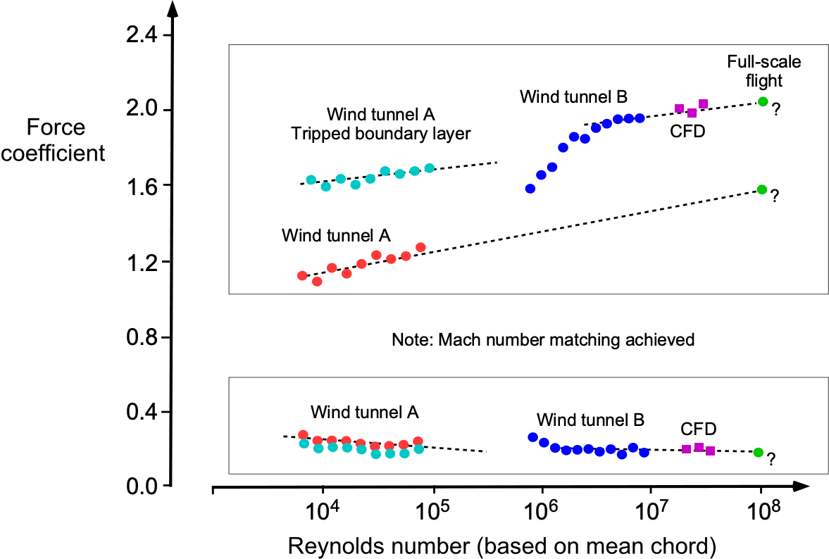
Reynolds number scaling of aerodynamic coefficients can be a satisfactory approach, especially if supported by CFD results.

However, discrepancies between wind tunnel and full-scale flight measurements may have causes that are more than just mismatching the similarity parameters. These causes may include the fidelity of the model shape, model support interference, wall corrections, aeroelastic effects, etc. Additionally, commonly used methods to simulate higher Reynolds number flows, such as artificially tripping the boundary layer, may also cause issues, resulting in an under-prediction or over-prediction of the full-scale values. Current approaches to wind-tunnel data extrapolation use computational fluid dynamics (CFD) solutions to help confirm the validity of any extrapolation process.

Similitude in Other Engineering Fields

As previously discussed, two systems can be considered geometrically, kinematically, and dynamically similar when all similarity parameters can be established to have the same numerical values, i.e., they are formally used to verify that the scaling of the problem has similitude. In practice, however, complete similarity is difficult to achieve when disparate geometric scales are involved, i.e., a very small model compared to the full-scale article. Nevertheless, the principles of dynamic scaling are essential because many engineering design processes become established when testing smaller models of the full-scale system(s).

Similitude analysis is a powerful design tool in fields other than aerodynamics. For example, scaling laws and similarity parameters can be derived in the fields of structures, structural dynamics, aeroelasticity, hydrodynamics, etc. The idea, again, is to scale the larger “real” or “full-scale” physical problem down to that of a model and/or a smaller prototype. If correctly done to match the similarity parameters governing the physics of the problem, it will then give the needed similarity of the physical behavior between the two disparate geometric scales.

However, just as in aerodynamics, designing a scaled-down structure (e.g., a wing or complete flight vehicle) that can match all of the problem’s similarity parameters is very challenging. Nevertheless, relaxing one or more scaling parameters may be appropriate, allowing at least partial similitude with a scaled model. To this end, parametric variations over some scales can sometimes expose the expected sensitivities of one parameter versus another and emphasize the more critical scaling parameter(s).

Structural & Aeroelastic Models

The behavior of an aircraft structure, such as a wing, depends on its stiffness, damping, and mass properties. In addition to force similitude, displacement similitude is usually enforced, so the model’s shape in the wind tunnel replicates that obtained during flight. For most flight vehicles, which have relatively large deformations, inertial, gravitational, and restoring forces will all be important in the design of a sub-scale model. Therefore, aeroelastically scaled models involving coupled aerodynamic-structure scaling can be designed to replicate their full-scale counterparts.

In this case, scaling a model that is aeroelastically similar to an aircraft requires that its characteristics under steady loads match those of the full-scale aircraft. i.e., a statically-aeroelastically scaled model deflects to the same shape and with scaled magnitude under the same scaled static loads. The question of what material a model should be made of is also a consideration. For example, it may not be possible to replicate a wing model using the same construction methods and materials as the full-scale wing.

The basic non-dimensional relationships governing the structural deformations can be found from dimensional analysis. If a lift force $L$ is applied to a cantilevered wing of semi-span ${s}$ , second moment of area $I$ , and modulus of elasticity, $E$ , then the tip deflection, $z_t$ , can be written in general functional form as

(20) $\begin{equation*} \frac{z_t}{s} = \phi \left( \frac{ I}{s^4}, \frac{ L}{E \, s^2} \right) \end{equation*}$

The lift force on the wing is proportional to the free-stream dynamic pressure, ${q_{\infty}}$ , and the wing reference (planform) area, $S$ , so the functional relationship can be reexpressed as

(21) $\begin{equation*} \frac{z_t}{s} = \phi \left( \frac{ I}{s^4}, \frac{ q_{\infty} \, S}{E \, s^2} \right) \end{equation*}$

Notice that $s^2/S$ (span squared divided by area) is the aspect ratio, $A\!R$ , so

(22) $\begin{equation*} \frac{z_t}{s} = \phi \left( \frac{ I}{s^4}, \frac{ q_{\infty}}{E \, AR } \right) \end{equation*}$

Therefore, the relevant similarity parameters governing the aeroelastic deformations of the wing are $z_t/s$ , $\ I/s^4$ , and $\ q_{\infty} /(E \, AR)$ . For aeroelastic scaling, these results are usually combined such that for dynamic similarity, then

(23) $\begin{equation*} \left( \frac{q_{\infty} \, s^4}{ AR \, E \, I} \right)_{\rm ms} = \left( \frac{q_{\infty} \, s^4}{ AR \, E \, I} \right)_{\rm fs} \end{equation*}$

where $E \, I$ is the wing stiffness or flexural rigidity, which can be rewritten as

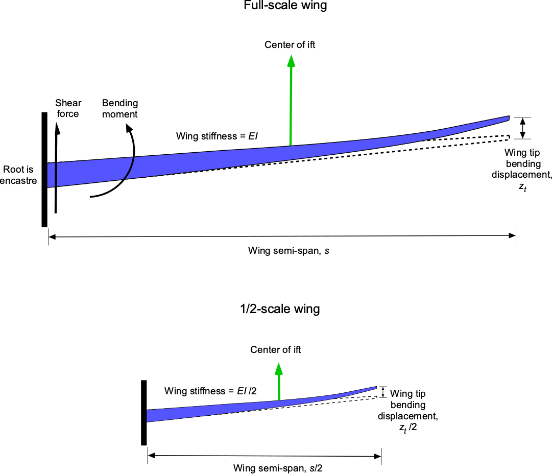
(24) $\begin{equation*} \left( \frac{(E \, I)_{\rm ms}}{( E \, I)_{\rm fs}}\right) = \left( \frac{q_{{\infty}_{\rm ms}}}{q_{{\infty}_{\rm fs}}}\right) \left( \frac{s_{\rm ms}}{s_{\rm fs}}\right) \left( \frac{AR_{\rm fs}}{AR_{\rm ms} } \right) \end{equation*}$

If geometric scaling is imposed, as it must be for dynamic similarity with the full-size flight vehicle, then

(25) $\begin{equation*} \left( \frac{(E \, I)_{\rm ms}}{( E \, I)_{\rm fs}}\right) = \left( \frac{q_{{\infty}_{\rm ms}}}{q_{{\infty}_{\rm fs}}}\right) \left( \frac{s_{\rm ms}}{s_{\rm fs}}\right) \end{equation*}$

Maintaining similarity using Eq. 25 will be required for faithful aeroelastic testing of a sub-scale model. For example, with a half-scale model being tested at the same dynamic pressure, the wing will have to have half the flexural rigidity of the full-scale wing. For testing at lower dynamic pressures, which is often the case in the wind tunnel, the wing stiffness must be reduced further. As shown in the figure below, the idea is to keep the wing deformations kinematically similar under the reduced aerodynamic loads. However, because such models are usually smaller than half-scale, the outcome is often a very flexible model that takes great care in manufacturing and testing.

In the aeroelastic testing of sub-scale wings, the wing deformations must be kinematically similar to full-scale, which requires a wing with reduced stiffness in bending and usually torsion.

In addition, for an aeroelastic model such as a wing, the Froude number, $F\!r$ , is usually relevant, which is defined as

(26) $\begin{equation*} F\!r = \frac{V_{\infty}}{\sqrt{ s \, g}} \end{equation*}$

The Froude number relates the aerodynamic inertial forces to the effects of gravity, which should also be matched to ensure dynamic similarity when wing flexibility, weight, and aeroelastic effects are relevant, i.e.,

(27) $\begin{equation*} \left( \frac{V_{\infty}^2}{ s \, g} \right)_{\rm ms} = \left( \frac{V_{\infty}^2}{ s \, g} \right)_{\rm fs} \end{equation*}$

In this regard, the Froude number determines the ratio of the deflections under a steady gravitational load to deflections resulting from aerodynamic and inertial loads.

Flutter Models

Flutter clearance is considered critical when developing new aircraft systems. As previously discussed, the interaction between aerodynamics and the structural response (often called structural dynamics) appears in terms of the ratio between forces induced by dynamic pressure relative to the structure’s stiffness for a given aspect ratio (required for geometric scaling), i.e.,

(28) $\begin{equation*} \frac{q_{\infty}}{E} \end{equation*}$

as well as mass density, which is the ratio of the structural mass, $M$ , to an appropriate volume grouping, i.e.,

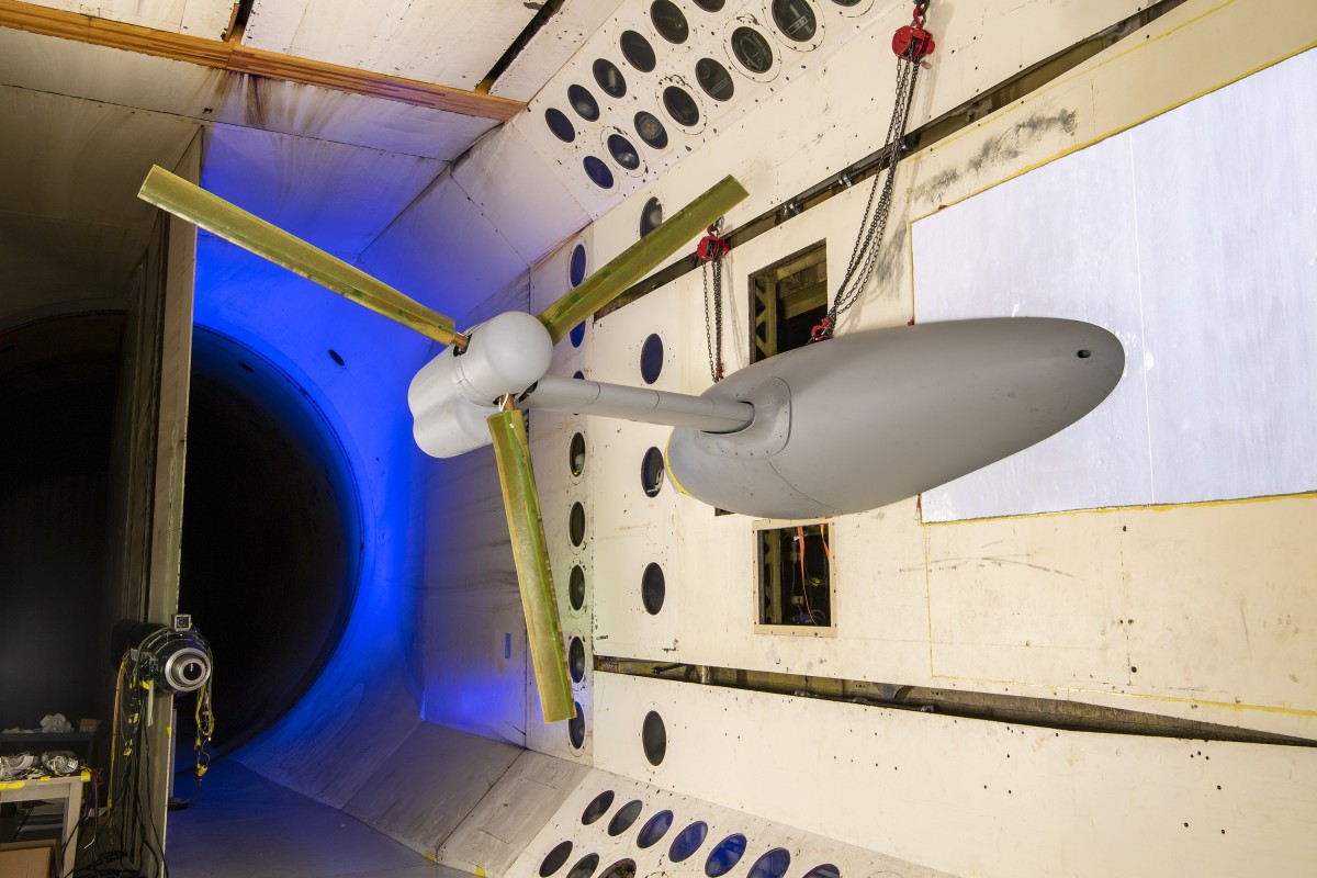
(29) $\begin{equation*} \frac{M}{s^3} \end{equation*}$

However, matching these ratios and similarity parameters usually results in a less stiff and more flexible model for aeroelastic and flutter testing. It is not unusual for flutter models to have segmented wing sections so that the wing has the necessary low stiffness in bending and torsion. The model may also have to operate at cryogenic temperatures, which can be challenging to manufacture. Nevertheless, a significant advantage of the wind tunnel approach is that measurements can be made at a smaller and more convenient physical scale to understand the effects of the primary problem parameters, validate mathematical models, and identify any potentially undesirable if not catastrophic, aeroelastic or flutter behavior that could manifest during the flight of the full-scale vehicle.

In the image below, a proprotor for a tiltrotor aircraft is mounted on a flexible, aeroelastically scaled wing to study the potential for whirl-flutter instability. This flutter is caused by coupling the proprotor aerodynamics and the proprotor’s dynamic response on the wing. The onset of whirl-flutter is often a limiting factor in a tiltrotor’s forward airspeed capability.

An example of a wing flutter model. In this case, a proprotor is mounted on a flexible, aeroelastically-scaled wing.

Aerodynamic time scales are also essential in aeroelasticity, i.e., the need to simulate the non-dimensional time scales of the model and the full-scale application. In this regard, the reduced frequency may be relevant regarding oscillatory behavior. For structural dynamic similitude, the dimensionless parameters pertinent to the scaled model are the reduced frequency, usually given the symbol $k$ , and the Froude number, $F\!r$ . Reduced frequencies are computed for a given airspeed considering the natural frequency of any given mode of vibration of the wing, $\omega$ (in units of radians per second), and the wing semi-span ${s}$ , i.e.,

$k = \frac{\omega\, b}{V_{\infty}}$

However, for transient time response the reduced time, $\hat{s}$ , may be more relevant, i.e.,

$\hat{s} = \frac{2 V_{\infty} \, t}{c}$

where $t$ is time and ${c}$ is the wing chord. A physical interpretation of this non-dimensional time is the distance the wing travels through the flow in terms of semi-chord lengths.

Hydrodynamic Models

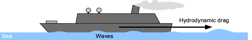
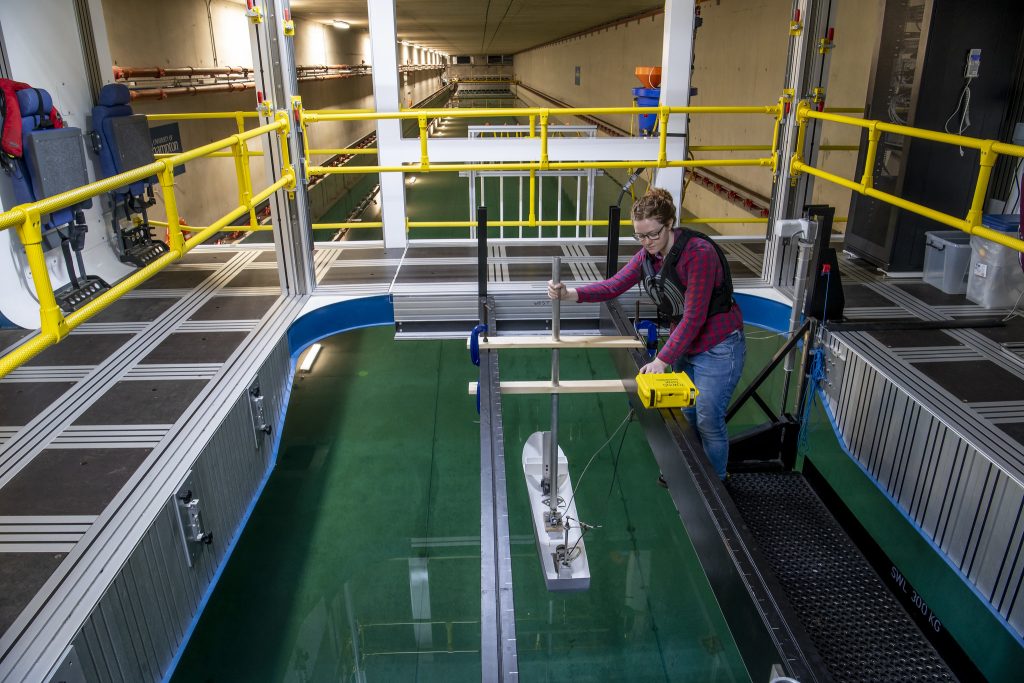
Designing a new ship, yacht, seaplane, etc., usually requires testing a sub-scale model in a towing tank. Tests may also be performed to improve the design of an existing or modified vehicle, such as to improve its performance, i.e., by reducing the hydrodynamic drag on a ship as it moves through the water. The hydrodynamic drag on a ship’s hull is caused by both viscous effects (from viscous shear on the hull) and gravitational effects (from wave motion). In the latter case, a ship traveling over a sea leaves behind it a train of waves, and because these waves possess an energy that is eventually dissipated, the ship experiences a wave drag force.

The hydrodynamic drag on a ship depends on its speed and wave height.

The drag coefficient on the hull of the ship can be written in functional form as

$C_D = \phi (Re, F\!r)$

where $Re$ is the Reynolds number based on ship length, ${l}$ , and the dimensionless grouping

$F\!r= \frac{V}{\sqrt{g \, l}}$

is the corresponding Froude number, where $V$ is the ship’s speed through the water. The resistance from viscous effects is a function of the Reynolds number and the roughness of the hull. In model ship testing, separating these two components (skin friction or shear drag and wave wake drag) makes it possible to determine the hydrodynamic drag of actual ships from tests done with smaller models, typically at 1:25 or 1:50 scale, such as in towing tanks.

The hydrodynamic drag on a ship can be estimated by testing a scaled model at or near the correct Reynolds number (which affects drag from viscous shear) and Froude number (which affects drag from wave motion).

If the hydrodynamic Froude number is much less than unity, implying that the waves’ wavelength is smaller than the ship’s length, then the resulting wave drag on the hull is comparatively small. If the ship’s length is equal to half the wavelength of the waves, the bow and stern waves interfere constructively, the so-called “hump speed” leading to a more significant value of wave drag. Therefore, a heavy ship with large volumetric displacement generally cannot overcome this peak in the wave drag, so its cruise speed will be limited.

High-speed boats, which can reach Froude numbers of over 3, can experience different regimes, eventually entering the so-called planing regime where they will skim over the water with significantly decreased drag. The same behavior occurs during the takeoff run of a seaplane when its weight eventually becomes supported by hydrodynamic lift rather than buoyancy, which is called operating “on the step.” Indeed, the ability of the seaplane to successfully take off from the water and fly depends on the ability of the pilot to reach this low hydrodynamic drag operating condition.

Check Your Understanding #2 – Reynolds & Mach numbers for a rocket

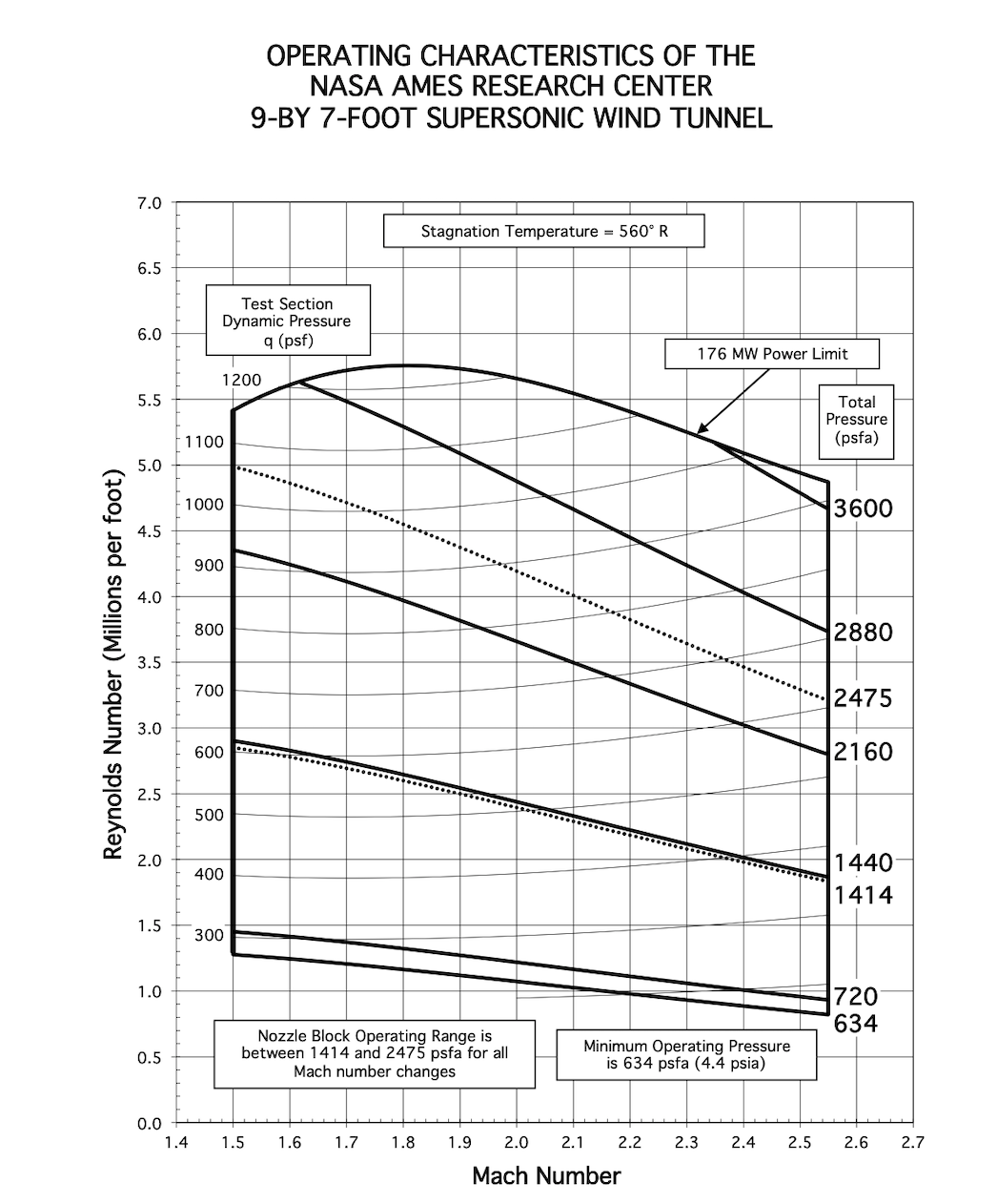
Estimate the Mach and Reynolds numbers (based on length) for a proposed launch vehicle near “max-q.” This condition is estimated to be a flight speed of 450 m/s at an altitude of 34,000 ft. The characteristic length of the actual launch vehicle is 134 ft. Next, considering the $Re$ and $M$ Maps for the NASA Unitary Plan Wind Tunnel, as shown below (click on the image for a bigger version), can these flight conditions be simulated in this wind tunnel using a sub-scale model of the launch vehicle? What scale might you recommend for the wind tunnel model and why? Which test section would you recommend? What might be done if the flight conditions cannot be replicated in this wind tunnel?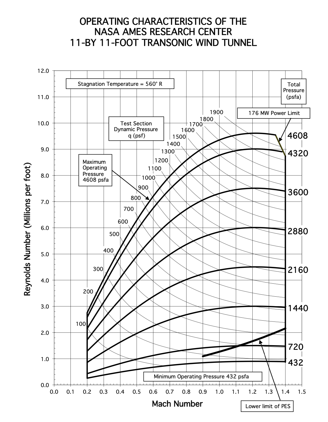

Show solution/hide solution.

At an altitude of 34,000 ft, the ISA standard values of the air properties are density $\varrho$ = 0.00076706 slugs ft ${^{-3}}$ , dynamic viscosity $\mu$ = 3.017 $\times 10^{-7}$ slugs ft $^{-1}$ s $^{-1}$ , speed of sound $a$ = 977.52 ft s $^{-1}$ . A flight speed $V$ of 450 m/s is 1,476.38 ft/s, so the flight Mach number is

$M = \frac{1,476.38}{977.53} = 1.51$

The corresponding Reynolds number based on the characteristic length is

$Re = \frac{\varrho \ V \ l}{\mu} = \frac{0.00076706 \times 1,476.38 \times 134.0}{3.017 \times 10^{-7}} = 5.03 \times 10^8$

or in terms of Reynolds number per foot, then

$Re = \frac{\varrho \ V }{\mu} = \frac{0.00076706 \times 1,476.38 }{3.017 \times 10^{-7}} = 3.75 \times 10^6~\mbox{per foot}$

Examining the $Re$ and $M$ Maps for the NASA Unitary Plan Wind Tunnel, the 9-foot-by-7-foot supersonic test section will give the required Mach number. The other transonic test section is capable of up to a Mach number of 1.4. The 9-foot-by-7-foot test section can also reach a Reynolds number of about 5 million per foot.

Generally, with a wind tunnel model, the largest dimension of the model needs to be no more than half of the largest dimension of the wind tunnel test section, which will give a tiny model in this case. However, for this type of slender (non-lifting) model, its length can be increased to no more than a smaller dimension of the wind tunnel test section, which is about 7 ft. Therefore, based on this length, the Reynolds number for the model will be about 35 million at a Mach number of about 1.51. While this is a reasonably high Reynolds number, it is still about one order of magnitude smaller than the actual flight Reynolds number.

It is known that, as far as the simulation of the aerodynamic conditions of supersonic flight is concerned, it is more important to simulate the Mach number than the Reynolds number. In this case, achieving the correct flight Mach number in the wind tunnel is possible. Moreover, while the Reynolds number is still lower, the effects of the Reynolds number at supersonic Mach numbers (at least if a certain minimum Reynolds number is achieved) are known to be secondary, so that the flight conditions can be adequately simulated in this wind tunnel. The results obtained will be faithful to the actual flight aerodynamics. This is another example of the challenges in sub-scale testing to study fundamental problems. However, with some ingenuity, the problem can be studied by matching the similarity parameters that govern the physics as closely as possible.

Summary of Similarity Parameters

Remember that similarity parameters quantify and analyze the physical similarity between systems, models, and full-scale articles. These parameters help engineers understand how the behavior of one system, such as a model, relates to another, often allowing for the prediction or analysis of physical phenomena from one scale to another. Below is a summary of some standard similarity parameters in aerospace engineering and their meanings.

1. Reynolds number, $Re$

$Re= \frac{\varrho \, V \, L}{\mu}$

where $\varrho$ is the density of the fluid, $V$ is the characteristic velocity, $L$ is the characteristic length, and $\mu$ is the dynamic viscosity of the fluid. The Reynolds number is used in fluid mechanics to characterize the flow of fluids (liquids or gases) around objects or through channels. It measures the ratio of inertial to viscous forces and helps predict flow regimes (e.g., laminar or turbulent) amongst other flow physics.

2. Mach number, $M$

$M = \frac{V}{a}$

where $V$ is the velocity of the object or fluid, and $a$ is the speed of sound in the medium. This parameter is significant in aerodynamics and compressible flow analysis. It is the ratio of the speed of an object (or fluid) to the speed of sound in the surrounding medium. It can also be used to classify flows and determine whether they are subsonic, transonic, supersonic, or hypersonic.

3. Froude number, $Fr$

$Fr = \frac{V}{\sqrt{g \, L}}$

where $g$ is the acceleration under gravity. The Froude number is a ratio of inertia forces to gravitational forces; it is used in hydrodynamics as well as aeroelasticity and flutter.

4. Weber number, $We$

$We = \frac{\varrho \, V^2 \, L}{\sigma}$

where $\sigma$ is the surface tension of the fluid. This parameter is used in fluid mechanics to characterize the importance of surface tension relative to inertial forces. It is commonly applied in studying fluid jets, droplet formation, and splashing phenomena.

5. Strouhal number, $St$

$St = \frac{f \, L}{V}$

where $f$ is the frequency of oscillation. It is used to analyze oscillating or vibrating flows, such as those found in vortex shedding behind bluff bodies.

6. Reduced frequency, $k$

$k = \frac{\omega \, c}{2 V}$

where $\omega$ is the circular frequency and ${c/2}$ is the semi-chord (of a wing). This parameter often appears in the field of unsteady aerodynamics and aeroelasticity.

7. Euler number, $Eu$

$Eu = \frac{p}{\varrho \, V^2}$

where $p$ is the pressure. This parameter helps analyze compressible flows. It is defined as the ratio of the pressure forces to inertial forces.

8. Prandtl number, $Pr$

$Pr = \frac{\mu \, C_p}{K}$

where $C_p$ is the specific heat at constant pressure, and $K$ is the thermal conductivity of the fluid. It characterizes the relative importance of molecular diffusion to momentum diffusion in a fluid. It is essential in heat transfer analysis, which helps predict convection heat transfer rates.

9. Grashof number, $Gr$

$Gr = \frac{g \beta (T_s - T_\infty) L^3}{\nu^2}$

where ${\beta}$ is the coefficient of volume expansion, $T_s$ , is the surface temperature, $T_\infty$ , is the ambient temperature, and $\nu$ is the kinematic viscosity of the fluid. It is a ratio of buoyancy to viscous forces and is significant in understanding phenomena like free convection around heated objects.

10. Leishman number, $Le$

$Le = \frac{m}{\varrho \, L^3}$

where $\varrho$ is the density of a fluid, $L$ is a characteristic length scale, and $m$ is the net mass of a body. This parameter represents the ratio of inertial effects to aerostatic buoyancy effects as it describes the dynamic motion of a body in air or water. The value is typically around unity in neutral buoyancy conditions. However, this parameter is unusually high for any body at rarefied atmospheric flight altitudes because of the lower air density.

Remember that using similarity parameters is fundamental in engineering analyses and can be used to understand and predict the scaling of various physical phenomena. The above list is inconclusive, and other similarity parameters may be helpful.

Summary & Closure

The principles encompassing geometric, kinematic, and dynamic similarity are used in all branches and disciplines of engineering. While developing appropriate similarity parameters that govern specific problems can take some work, the benefits to the engineer are usually significant. Similarity parameters not only help generalize the system’s behavior but also allow the engineer to reduce the scope of the problem, i.e., by reducing the number of dependent parameters to consider in the design process, especially when there are many. Therefore, similarity parameters can help transfer data and results from one (e.g., smaller) scale to another (e.g., full-scale application).

Using similarity parameters and the principles of dynamic similarity is an essential tool in designing and optimizing engineering systems across many industries. One significant benefit of using and matching similarity parameters is replicating a particular physical behavior at a smaller scale, where it can be more carefully studied, e.g., by testing in a wind tunnel. For example, a physical model or wind tunnel test can be used to study the aerodynamics of a full-scale aircraft, and the results obtained can then be scaled to the actual conditions the aircraft will face in flight. However, scaling the flow properties, especially the Reynolds number, can be challenging at a smaller scale, so one solution is to use another fluid (or gas) in the wind tunnel. However, this approach has many practical challenges, including using a special wind tunnel to contain the gas. Nevertheless, this type of approach allows engineers to obtain valuable information and make predictions about the behavior of the aircraft without the need to construct prototypes and conduct expensive, full-scale flight tests.

While using similarity parameters is not limited to wind tunnels, testing scaled models of aerospace systems can be very valuable in the engineering design process. This approach can help identify potential problems that can be addressed at an early stage rather than being discovered when the actual system is fielded. For example, predicting flutter on flight vehicles is essential to ensure the structural design is stiff enough and lightweight.

5-Question Self-Assessment Quickquiz

For Further Thought or Discussion

Discuss some challenges of using a gas other than air to achieve dynamic flow similarity with a scale model in a wind tunnel.
Do some research to determine the purpose of a cryogenic wind tunnel for testing scaled models.
Discuss how computational methods, such as computational fluid dynamics (CFD), might achieve similitude in virtual environments, reducing the need for physical models.
What is “flutter”? Do some research to determine why the potential for flutter can be a severe problem in airframe design.
Aeroelastic models are sometimes called “Froude-scaled models.” What might be the governing similarity parameter in this case?
Emphasize the importance of dynamic similarity in engineering design and safety assessments, where understanding how a system will behave under different conditions is critical.

Other Useful Online Resources about Dynamic Similarity

Wikipedia pages on similitude and dynamic similarity.
A video on dynamic similarity in fluid dynamics.
A video lecture with a review of dimensional analysis and similitude.
A video lecture from the University of Colorado on similitude and scaling.
This is an excellent video on what causes flutter.
Archival film from NASA Langley Research Center’s 16-Foot Transonic Dynamics Tunnel. Composite of several tests on propeller whirl and flutter of helicopter blades.
Video of small-scale tiltrotor whirl flutter tests.

License

Icon for the Creative Commons Attribution-NonCommercial-NoDerivatives 4.0 International License

Introduction to Aerospace Flight Vehicles Copyright © 2022–2025 by J. Gordon Leishman is licensed under a Creative Commons Attribution-NonCommercial-NoDerivatives 4.0 International License, except where otherwise noted.

Digital Object Identifier (DOI)

https://doi.org/https://doi.org/10.15394/eaglepub.2022.1066.n14