13 Atmospheric Properties & the ISA
Introduction
The performance of any atmospheric flight vehicle is affected by the density of the air in which it is flying. The pressure, temperature, and density of the air in the atmosphere are all functions of altitude. In particular, air density affects the aerodynamic performance of an aircraft in terms of its lift and drag, as well as the thrust and/or power output from its engine(s). Furthermore, determining the aerodynamic forces on a launch vehicle is crucial during its flight within the lower parts of the atmosphere, as well as spacecraft that fly in the high atmosphere during re-entry. Finally, the readings on aircraft instruments, such as the altimeter and the airspeed indicator, which are pneumatic (i.e., respond to air pressure), also depend on the local fluid properties found in the atmosphere.
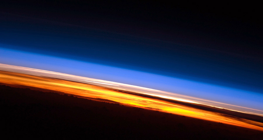
The layered, shell-like structure of the Earth’s atmosphere is visible in the photograph shown below, which was taken at sunset over the Indian Ocean from the International Space Station. The troposphere (orange) is at the bottom, above the darkness of the Earth’s surface. The troposphere, which comprises approximately 80% of the Earth’s atmosphere by mass, is the region where winds and weather phenomena predominantly occur. It is within this layer that all human activity and existence have transpired. Above this lies the pink-to-white colored zone, known as the stratosphere, where the ozone layer resides and protects the Earth from harmful UV radiation.[1] Higher still is the mesosphere, a shell that appears as light blue in this image, and beyond that, it gradually fades into the thermosphere and the darkness of space. Notably, the thickness of the majority of the atmosphere is only about 1.6% of the Earth’s radius.
It should also be appreciated that weather and winds cause the properties of the atmosphere to vary from place to place over the Earth, from day to day, and even from hour to hour. Therefore, one problem that arises immediately is the development of a means to standardize the properties of the atmosphere for use in various measurements, as well as for both engineering and aviation purposes. This issue is why defining a standard atmospheric model, known as the International Standard Atmosphere (ISA), is necessary.
Learning Objectives
- Know more about the composition and properties of the Earth’s atmosphere as a function of altitude or “height” from the surface.
- Understand why a “standard” atmospheric model needs to be defined for use in engineering analysis and other areas of practical aviation.
- Be able to calculate air properties in the International Standard Atmosphere (ISA) using the ISA equations and read the relevant properties from a table.
- Know how to use the hydrostatic equations to help estimate the atmospheric properties of other planets.
Composition of the Atmosphere
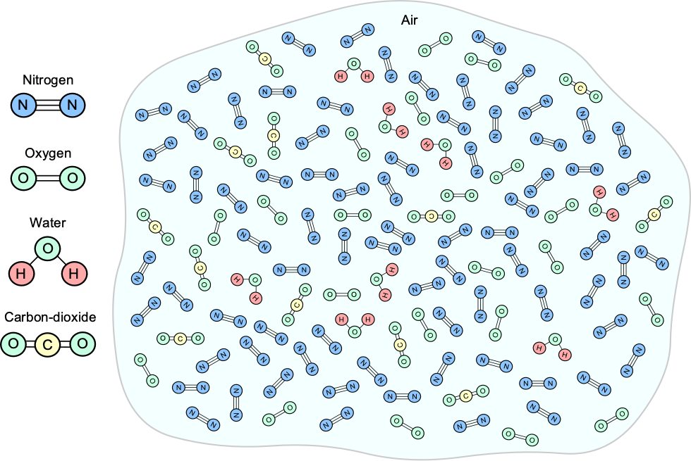
Aeronautical engineers are primarily concerned with the properties of air in the lower atmosphere, specifically the troposphere, where aircraft typically fly. In this regard, the relevant properties are pressure, temperature, density, viscosity, and the speed of sound. Air represents a mixture of several gases by volume, namely nitrogen (78%), oxygen (21%), noble gases (0.9%), carbon dioxide (less than 0.1%), and other trace gases. The natural winds and turbulence in the lower atmosphere keep these gases well-mixed, as illustrated in the figure below. Other natural atmospheric materials include water vapor, dust particles, smoke, viruses, bacteria, etc. Many dust particles, known as aerosol particles or aerosols, originate from volcanic sources. Like smoke, they remain suspended for a long time because of their tiny sub-micron size.
The figure below illustrates that as one moves up in the atmosphere, away from the Earth’s surface, the atmosphere naturally forms a series of strata, or “shells,” where the air has distinct characteristics and properties. The troposphere is flattened towards the poles because of the centrifugal effects caused by the Earth’s rotation around its orbital axis. Astronautical engineers are primarily concerned with the atmospheric properties above the tropopause and into the stratosphere and mesosphere. Above the tropopause, the temperature and other atmospheric properties change differently with height or altitude compared to those in the troposphere.
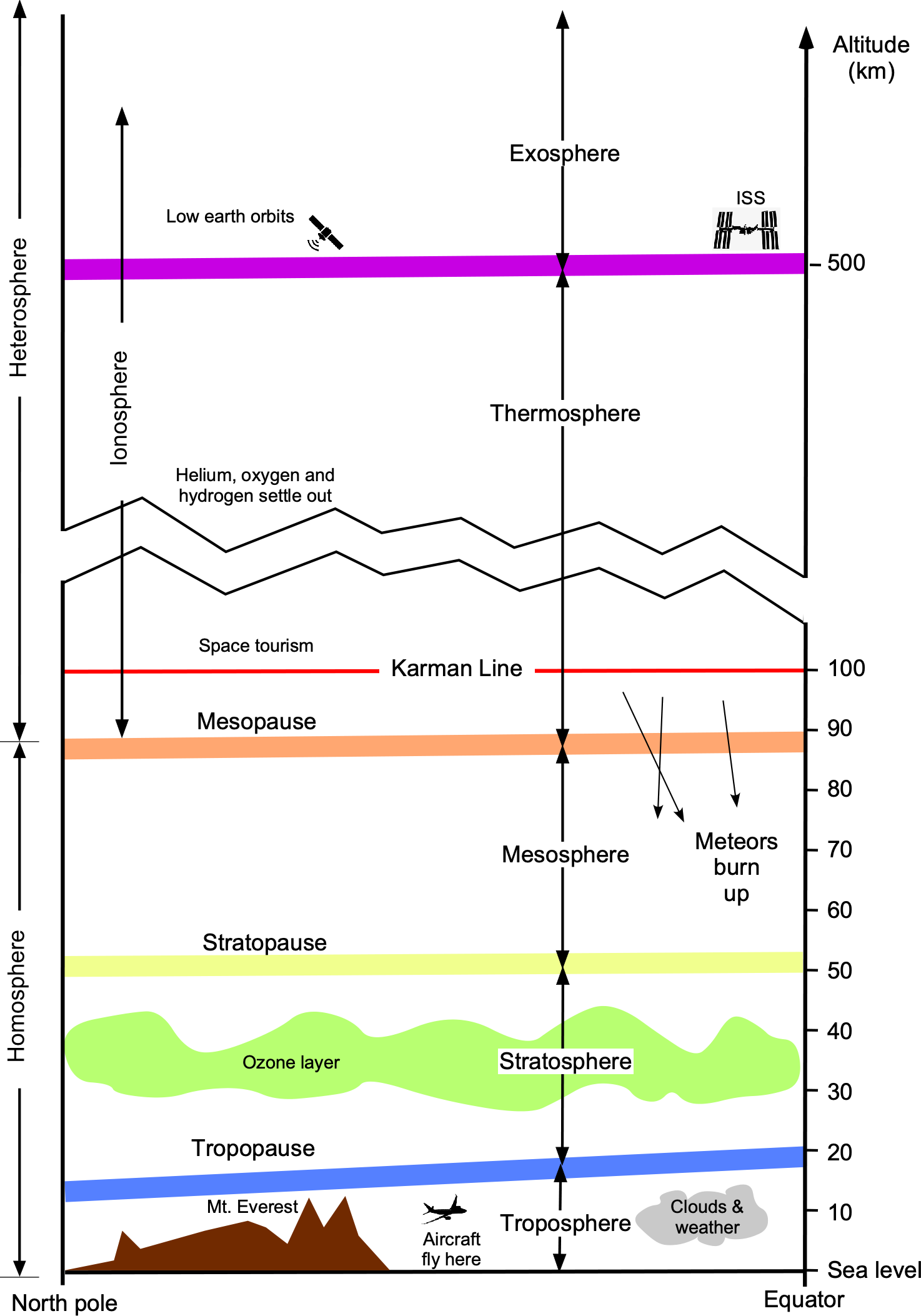
At higher altitudes above 300,000 ft (90 km), the different gases also begin to settle or separate into shells according to their respective densities, namely oxygen (heaviest), helium, and hydrogen (lightest). The edge of space is typically defined as 100 km (approximately 62 miles or 328,000 ft), often referred to as the Kármán Line. Although the Kármán line is an arbitrary boundary, it is widely recognized and used as a standard in the aerospace industry. It is also the reference altitude used by the Fédération Aéronautique Internationale (FAI) to define the edge of space.
General Properties of the Atmosphere
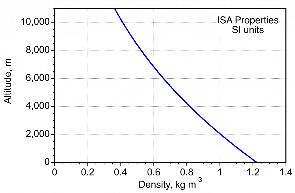
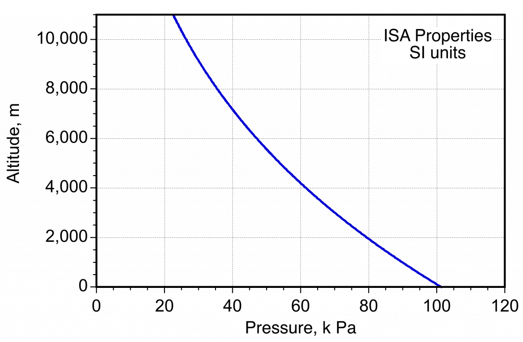
The figure below illustrates the variations in temperature, pressure, and density of the atmosphere with height or altitude. Both pressure and density decrease quickly and asymptotically with altitude above mean sea level (MSL), which is not surprising because pressure is directly related to the weight of air above; there is less air above when going higher into the atmosphere.
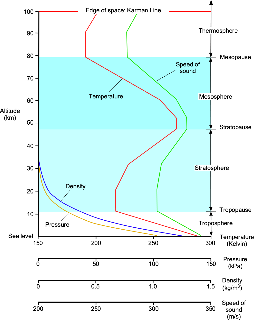
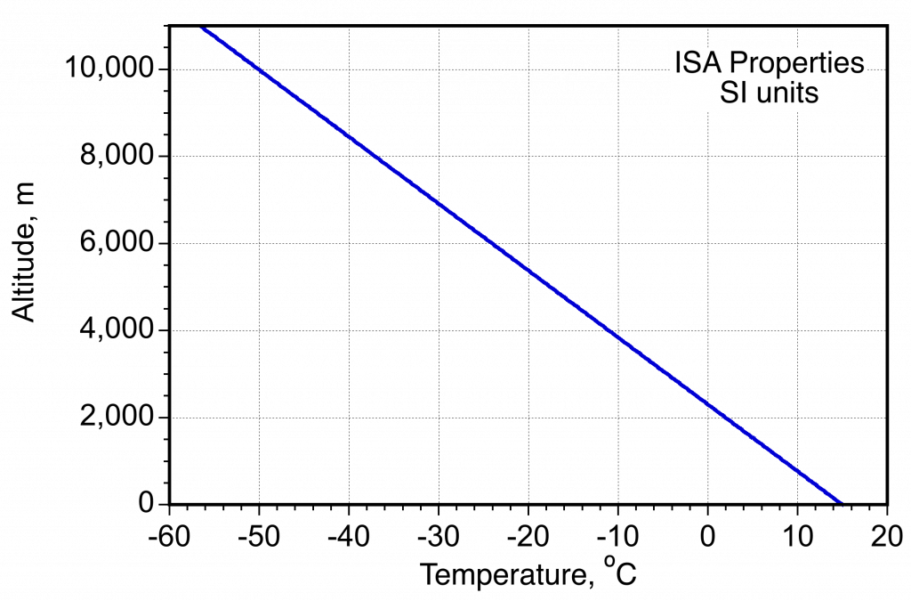
The temperature in the entire atmosphere is more complicated to describe. There are regions where the temperature increases with increasing height and regions where the temperature decreases with increasing height. The temperature decreases approximately linearly with height in the troposphere (below 36,000 ft or 11,000 m). However, the actual lapse rate can vary daily and from place to place over the Earth. The region above the troposphere is called the stratosphere. In this region, temperature increases with increasing height because solar radiation affects this part of the atmosphere containing the ozone layer.
What is the ozone layer?
The ozone layer is a shell of the Earth’s stratosphere, located approximately 10 to 50 kilometers above the surface. It contains a high concentration of ozone (O3) molecules, which are formed when oxygen (O2) molecules are exposed to ultraviolet (UV) radiation from the Sun. The ozone layer plays a crucial role in protecting life on Earth by absorbing most of the Sun’s harmful UV radiation, particularly the high-energy UV-B and UV-C rays. The discovery of the ozone layer and its significance in the Earth’s climate during the 1970s led to international efforts to reduce the use of ozone-depleting substances, such as chlorofluorocarbons (CFCs), which are now mostly banned.
Reasons for the ISA model
The International Standard Atmosphere (ISA) model represents an average, ideal atmosphere. It is based on thermodynamic relationships (equation of state) and assumes that the atmosphere lacks water vapor, wind, and turbulence. The ISA has been established to provide a common reference standard for the lower atmosphere (i.e., the troposphere) in terms of pressure, temperature, density, and other properties such as viscosity and the speed of sound.
The ISA model is necessary for the aerospace industry because it provides a standardized reference for calculating and testing aircraft and engine performance. With the ISA, engineers can predict and compare the performance of different aircraft designs under the same standard atmospheric conditions, making it easier to compare the performance of other aircraft and engines. In addition to its use in performance calculations, the ISA is also a reference for instrument calibration. By calibrating instruments such as altimeters and airspeed indicators relative to the ISA, all such instruments will show identical readings under the same atmospheric conditions, regardless of the actual conditions on any given day or time.
It is essential to recognize that the ISA model is not a meteorological model of actual atmospheric conditions, such as those derived from barometric pressure changes or wind conditions. Neither does it account for humidity effects; the air in the ISA model is assumed to be dry, clean, and of constant composition. However, humidity effects are typically accounted for in the flight vehicle performance or engine analysis by applying a correction factor after obtaining the pressure and density from the ISA model, as discussed later in this chapter.
The International Organization for Standardization (ISO) publishes the ISA model as International Standard ISO 2533:1975. The International Civil Aviation Organization (ICAO) has also adopted the ISA model, which is used universally throughout all aspects of civil aviation. A document on the ISA standard can also be obtained from NOAA. Tables of ISA properties are published for discrete altitude values incremented in a few hundred feet or meters in many sources, including almost every textbook on aerodynamics and aircraft performance. These ISA tables can be used to find appropriate values at intermediate altitudes by using linear interpolation, recognizing that this process is straightforward yet approximate. A much better approach, in general, is to calculate the properties for any specified altitude using the equations of the ISA, which will now be determined.
Geopotential Altitude vs Geometric Altitude
It is important to distinguish between geometric altitude and geopotential altitude. The ISA model uses the geopotential altitude. The geometric altitude, denoted  , is the actual vertical distance above MSL. It is the physical height one would measure with a ruler or tape measure, or an output from a GPS, and corresponds directly to the spatial position of an object above the Earth’s surface. Geopotential altitude, denoted by
  , assumes that gravity remains constant at its sea-level value for all heights, i.e.,
  . This approach defines a reference value of altitude, , such that the gravitational potential energy at that altitude (per unit mass) matches the potential energy calculated using a reduction in the value of
  with altitude. Mathematically, the relationship can be expressed as
(1) 
where  is the local gravitational acceleration under gravity at some geometric height , and
  is the MSL value. Because depends on the distance above the surface of the Earth, the geopotential altitude is related to the geometric altitude using the universal law of gravitation, which gives
(2) 
where  = 6.371
  10
10 m (2.0902 10
 ft) is the mean radius of the Earth. This latter expression shows that
  for all
  , and that the two values become increasingly different at higher altitudes. The difference between the two altitudes is a result of the small reduction in the acceleration under gravity with height from the Earth’s surface, which is given by
(3) 
For lower altitudes  , then
  is very small and can often be neglected. At typical commercial flight altitudes, e.g.,
  = 10,000 m to 12,000 m (approximately 1,000 ft to 40,000 ft), the difference between and is only about 15 to 20 meters (49.2 to 65.6 ft), i.e., less than 0.2%. This difference is negligible for most practical flight and engineering applications. When is much smaller than , then the correction
(4) 
can be used, which is valid at low to moderate altitudes. Up to approximately 20 km (65,000 ft), the difference between geopotential and geometric altitude is small, less than 0.5%, which is well within the tolerances for navigation, flight performance, and terrain avoidance. However, at high altitudes relevant to rocketry and satellite dynamics, e.g., = 300,000 m (9.842 10 ft) or more, the difference becomes hundreds of meters (or several hundred feet). Therefore, for any application requiring precise modeling of the vertical structure of the atmosphere beyond the troposphere, it becomes more important to distinguish between geometric and geopotential altitudes.
Check Your Understanding #1 – Calculating geometric altitude from geopotential altitude
Given a geopotential altitude of = 10,000 m, which was measured with an altimeter, compute the corresponding geometric altitude .
Show solution/hide solution.
The geometric altitude is related to the geopotential altitude by
![\[ h_g = \frac{h R_E}{R_E - h} \]](https://eaglepubs.erau.edu/app/uploads/quicklatex/quicklatex.com-f1cdb8c10af0ca5a12a3e91e32cb3612_l3.svg "Rendered by QuickLaTeX.com")
Substituting the numerical values gives
![\[ h_g = \frac{10{,}000 \times 6.371 \times 10^6}{6.371 \times 10^6 - 10{,}000} = 10,015.7~\text{m} \]](https://eaglepubs.erau.edu/app/uploads/quicklatex/quicklatex.com-219b7d6848c82bdd61c353aaa99c5a75_l3.svg "Rendered by QuickLaTeX.com")
Therefore, a geopotential altitude of 10,000 m corresponds to a geometric altitude of approximately 10,015.7 m, i.e., a difference of only 15.7 m. Therefore, for most practical applications in aviation and flight analysis, the difference between geometric and geopotential altitude is negligible and may be safely ignored.
Equations of the ISA in the Troposphere
The equations of the ISA can be established starting from the hydrostatic equation, which has already been introduced, i.e., using
(5) 
Remember that the hydrostatic equation is an ordinary differential equation that relates the change in pressure,  , in a fluid with respect to a change in geopotential altitude or height,
  . Typically, when discussing the atmosphere, the symbol is used instead of
  to represent “height” or altitude. In this case, the height is measured relative to Mean Sea Level (MSL).
Temperature Variation
The temperature  in the standard atmosphere is assumed to be a linearly decreasing function of altitude, which is a good statistical approximation to the actual average temperature variation in the atmosphere and can be expressed by
(6) 
or
(7) 
In this case, is expressed in feet (ft), and  is a constant known as the standard atmospheric lapse rate. This temperature lapse equation is valid only to the troposphere’s limits, or approximately 36,000 ft, which is known as the tropopause. After that, the temperature stays constant, up to about 65,000 ft.
The value of is 3.57 F per 1,000 ft of altitude or 0.00357F per ft = 0.00357R per ft. In practice, lapse rates will change with the level of humidity. The dry adiabatic lapse rate is about 5.5 F per 1,000 ft of altitude, and the moist lapse rate ranges varies between 2–3 F per 1,000 ft of altitude; the ISA model uses an accepted standard value of lapse rate that is between these two other lapse rates.
In SI units, the atmospheric temperature lapse equation can be written as
(8) 
or
(9) 
where is expressed in meters (m), and the lapse rate, in this case, is 6.5C per 1,000 m. This lapse rate is equivalent to 1.981C per 1,000 ft, giving
(10) 
with being measured in feet (ft). It is standard practice to measure altitude in feet for aeronautical and aviation purposes, although, if needed, the conversion is 1 meter (m) = 3.28084 feet (ft). It is essential to ensure the value of the lapse rate is expressed in the units of interest. Often, the ratio of the ISA temperature at a given altitude to the MSL temperature is used, which is given the symbol  , i.e.,
(11) 
Solutions for Pressure & Density
In summary, three equations are now available:
1. The hydrostatic equation, which is an ordinary differential equation, i.e.,
(12) 
2. An equation for the linear temperature variation or lapse with height, i.e.,
(13) 
3. The thermodynamic equation of state, i.e.,
(14) 
Substituting the latter two equations (Eqs. 13 and 14) into the hydrostatic equation (Eq. 12) gives
(15) 
which is the governing equation that now needs to be solved.
Solution for Pressure
Using separation of variables and integrating between MSL ( ) and the height of interest, where the pressure is
  gives
gives
(16) 
The left-hand side integrates to
(17) 
and the right-hand side is a standard integral, i.e.,
(18) 
Therefore, after integrating, it gives
(19) 
and exponentiating both sides yields
(20) 
ISA Pressure Variations
The resulting pressure in the ISA, , at any altitude relative to the value at MSL,  , becomes
(21) 
where in this latter equation is measured in feet (ft). Notice that in USC, then
(22) 
Remember that  is the gas constant for air, which is 1716.49 ft-lb slug
 R or 287.057 J kg K. Therefore, the value of
  , which is a non-dimensional grouping, is
(23) 
so its numerical value does not depend on the unit system. If were to be measured in meters (m), then
(24) 
where, in this case
(25) 
Under standard MSL conditions, the value of is 2116.4 lb/ft , 101,325 N/m
 , or 101,325 Pa or 101.325 kPa.
Solution for Density
The corresponding density ratio can also be determined. From the equation of state, i.e.,
(26) 
Notice that the temperature lapse in Eq. 13 can be written as
(27) 
so that
(28) 
ISA Density Variations
The corresponding density  in the ISA at any altitude can be calculated by invoking the thermodynamic equation of state, i.e., Eq. 26. If the local temperature corresponds to the standard local temperature in the ISA, i.e.,
  , then
(29) 
and so the local density in the ISA relative to MSL is
(30) 
where is measured in feet (ft). If is measured in meters (m), then
(31) 
Notice that  is dimensionless and equal to 5.256. Recall that under standard MSL conditions the value of
  is 0.002378 slugs/ft
 or 1.225 kg/m
 .
.
Summary of ISA Properties at MSL
The values of the ISA properties at standard MSL conditions are helpful to have on hand and are provided in the table below.
| Property | Symbol | SI units | USC units |
| Pressure | |
1.0132510 Nm Nm (Pa) (Pa) |
2116.4 lb/ft (29.92 inches of Hg) |
| Density | |
1.225 kg m |
0.002378 slugs ft |
| Temperature |  |
288.15 K | 518.67 R |
| Dynamic viscosity |  |
1.78910 kg m s kg m s |
3.73710 slugs ft s slugs ft s |
| Speed of sound |  |
340.3 m s |
1116.47 ft s |
| Gas constant | |
287.057 J kg K |
1716.49 ft-lb slugR |
ISA Summary – Temperature, Pressure, and Density Relations
The following summarizes the ISA temperature, pressure, and density relationships in both SI and USC units.
Temperature
- USC Units:
![\[ T = T_0 - B \, h = 59.0 - \left( \frac{3.57}{1{,}000} \right) h = 59.0 - 0.00357 \, h \quad \text{in $^\circ$F, with ${h}$ in ft} \]](https://eaglepubs.erau.edu/app/uploads/quicklatex/quicklatex.com-1e908ead0e10c1c7164a822b27fd3ab6_l3.svg "Rendered by QuickLaTeX.com")
- SI Units:
![\[ T = T_0 - B \, h = 15.0 - \left( \frac{6.5}{1{,}000} \right) h = 15.0 - 0.0065 \, h \quad \text{in $^\circ$C, with ${h}$ in m} \]](https://eaglepubs.erau.edu/app/uploads/quicklatex/quicklatex.com-2c256c11bd821014e524595e3de7ff18_l3.svg "Rendered by QuickLaTeX.com")
- Alternate: SI temperature with in ft:
![\[ T = 15.0 - 0.001981 \, h \quad \text{in $^\circ$C, with ${h}$ in ft} \]](https://eaglepubs.erau.edu/app/uploads/quicklatex/quicklatex.com-83b317a99771fa93c5048a3531ede870_l3.svg "Rendered by QuickLaTeX.com")
Pressure
- SI Units:
![\[ \delta = \left( 1 - 6.883 \times 10^{-6} \, h \right)^{5.256} \quad \text{with ${h}$ in m} \]](https://eaglepubs.erau.edu/app/uploads/quicklatex/quicklatex.com-bd749a78004dffc7a7f6412b703c0781_l3.svg "Rendered by QuickLaTeX.com")
- USC Units:
![\[ \delta = \left( 1 - 2.256 \times 10^{-5} \, h \right)^{5.256} \quad \text{with ${h}$ in ft} \]](https://eaglepubs.erau.edu/app/uploads/quicklatex/quicklatex.com-c539d7bbe95bbe02f8c74b4a80da9586_l3.svg "Rendered by QuickLaTeX.com")
Density
- SI Units:
![\[ \sigma = \left( 1 - 6.883 \times 10^{-6} \, h \right)^{4.256} \quad \text{with ${h}$ in m} \]](https://eaglepubs.erau.edu/app/uploads/quicklatex/quicklatex.com-010503573e75a25326b5080fc447651d_l3.svg "Rendered by QuickLaTeX.com")
- USC Units:
![\[ \sigma = \left( 1 - 2.256 \times 10^{-5} \, h \right)^{4.256} \quad \text{with ${h}$ in ft} \]](https://eaglepubs.erau.edu/app/uploads/quicklatex/quicklatex.com-06b266f2d43acdc979d8998f20ae41cc_l3.svg "Rendered by QuickLaTeX.com")
Check Your Understanding #2 – Calculation of the properties of the ISA
Calculate the properties of the ISA using the relevant equations. You may do this in SI or USC units, but it is best to try to calculate the properties in both sets of units. Assume the altitude is the geopotential altitude.
Show solution/hide solution.
The equations for the ISA are relatively easy to program in MATLAB; below is a short piece of code used to calculate such properties in the troposphere.
g0=9.81; % MSL reference value of acceleration under gravity in m/s^2
B=-0.0065; % temp lapse rate in ISA in Kelvin/meter
R=287.05; % gas constant for air
T_sl=288.15; % ISA MSL standard temperature in Kelvin
p_sl=1.01325e+5; % standard pressure at sea level in Pascals
rho_sl=p_sl/(R*T_sl) % use the ideal gas law to get the density
a_sl=sqrt(1.40*p_sl/rho_sl) % speed of sound at sea level
z=linspace(0,10000,1000); % z is geopotential altitude, so calculate ISA properties up to the tropopause
T_z=T_sl+B.*z;
p_z=p_sl.*((1+B.*z./T_sl).^(-g0/(R*B)));
rho_z=p_z./(R.*T_z);
mu_z=1.458e-6.*sqrt(T_z)./(1.0+0+110.40./T_z); % Sutherland’s law
a_z=sqrt(1.40.*p_z./rho_z); % speed of sound or use a_z=sqrt(1.40.*R*T_z)
- Variation of density in the ISA measured in SI units.
- Variation of pressure in the ISA measured in SI units.
- Variation of temperature in the ISA measured in SI units.
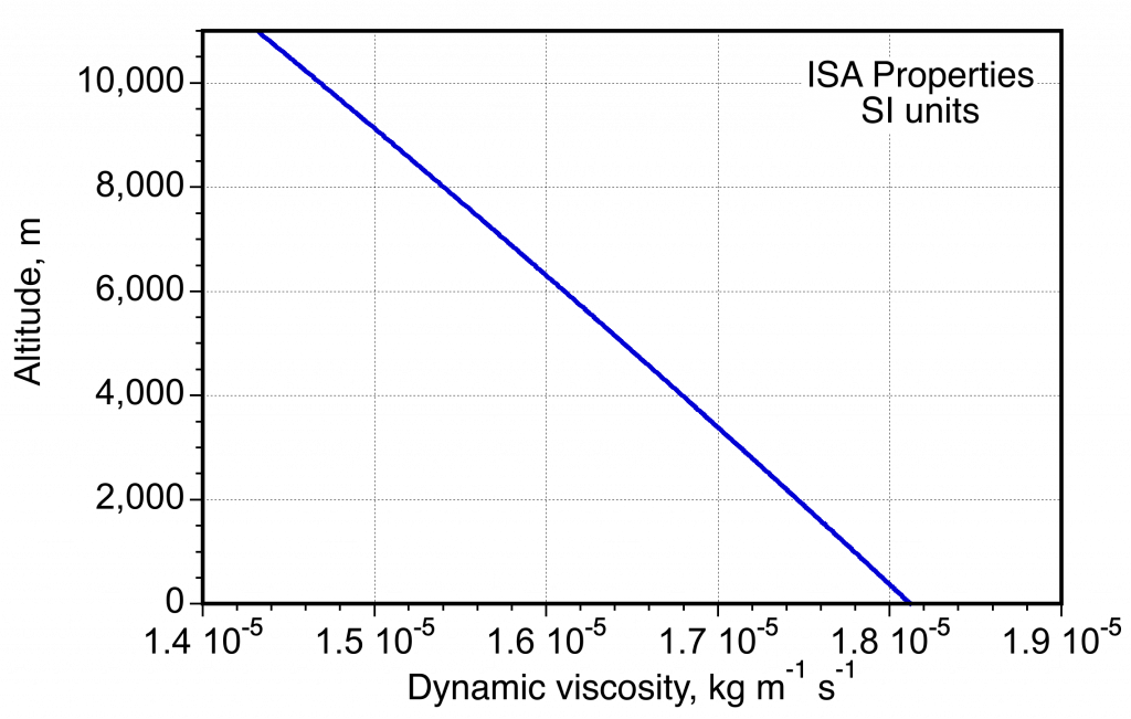
- Variation of viscosity in the ISA measured in SI units.
Pressure Altitude and Density Altitude
In flight operations, the concepts of pressure altitude and density altitude are used to describe an aircraft’s effective altitude relative to the ISA. Pressure altitude, denoted  , is the altitude in the ISA model at which the standard atmospheric pressure equals the actual atmospheric pressure. It is determined from the barometric pressure reading corresponding to the standard sea-level pressure of 1013.25 hPa (101,325 Pa, 101.325 kPa, 1013.25 mbar) in SI units or 2,116.4 lb/ft (29.92 inches of Hg) in USC units. Rearranging the pressure ratio equation to solve for height gives
(32) 
Density altitude, denoted  , is the altitude in the ISA model at which the standard atmospheric density equals the actual air density at the point of interest. It is a function of both pressure and temperature, and is used to assess aircraft performance because aerodynamic and engine behavior depend strongly on air density. The density altitude can be solved by rearranging the standard ISA density equation, i.e.,
(33) 
where = 1.225 kg/m is the standard sea-level density in SI units or 0.002378 slugs/ft in USC units.
In practical aviation terms, higher-than-standard temperatures or lower-than-standard pressures cause the density altitude to increase, meaning the aircraft behaves as if it were flying at a higher geometric altitude in the standard atmosphere. This condition reduces engine power, aerodynamic lift, and climb performance. Pilots must account for density altitude, especially in hot-and-high conditions or when calculating takeoff and climb capability. Analysis of the governing equations shows that the density altitude exceeds the pressure altitude by approximately 55 feet for every 1 F that the actual temperature exceeds the standard ISA temperature at that altitude. In SI units, this corresponds to a density altitude increase of about 30 meters for each 1C of temperature above standard. An approximate formula for estimating this effect is
(34) 
where is the actual outside air temperature (OAT),  is the standard temperature at pressure altitude , and
  is a constant = 55 ft/F in USC units or 30 m/C in SI units. This latter expression provides a quick operational estimate of how temperature deviations from standard impact aircraft performance through changes in air density.
It will be noticed that if the local temperature corresponds to the standard temperature at that altitude, then the pressure altitude and the density altitude are the same, i.e.,  , which follows directly from the equations for pressure and density altitude. Assume the actual temperature equals the standard ISA temperature at the pressure altitude, i.e.,
  . From the equation of state, then
(35) 
Substituting this into the density ratio, giving
(36) 
and substituting this into the density altitude equation gives
(37)
the same expression as for is recovered, confirming that  when
when  .
.
Check Your Understanding #3 – Estimating density altitude
Given that the pressure altitude is  ft and the outside air temperature
  F, then calculate the density altitude in both USC and SI units.
Show solution/hide solution.
- USC solution: The ISA temperature is
![\[\]](https://eaglepubs.erau.edu/app/uploads/quicklatex/quicklatex.com-4aabddc1c342c8ef16735dbd83bd3e5b_l3.svg "Rendered by QuickLaTeX.com")
![\[ T_{\text{ISA}} = 59 - 0.00357 \times 6,000 = 37.58^\circ\text{F} \]](https://eaglepubs.erau.edu/app/uploads/quicklatex/quicklatex.com-ad8b9c78bca9baa02bd86e78ceccaa00_l3.svg "Rendered by QuickLaTeX.com")
Using the approximate method, then
![\[ h_\varrho \approx h_p + 55 (T - T_{\text{ISA}}) = 6,000 + 55 \times 40.42 = 8,223~\text{ft} \]](https://eaglepubs.erau.edu/app/uploads/quicklatex/quicklatex.com-0e75c4d07d7711ef2c5db86f47b229ca_l3.svg "Rendered by QuickLaTeX.com")
and with the exact method
![\[ \delta = \left(1 - 2.256 \times 10^{-5} \times 6,000 \right)^{5.256} = 0.7842 \quad \text{and} \quad \sigma = \frac{0.7842}{537.67 / 518.67} = 8,340~\text{ft} \]](https://eaglepubs.erau.edu/app/uploads/quicklatex/quicklatex.com-fdae94f4d286259cff1a2b8f5ebf3e19_l3.svg "Rendered by QuickLaTeX.com")
- SI solution: In this case, a conversion to SI gives = 1,829 m and = 25.6C. The ISA temperature is
![\[ T_{\text{ISA}} = 15 - 0.0065 \times 1,829 = 2.61^\circ\text{C} \]](https://eaglepubs.erau.edu/app/uploads/quicklatex/quicklatex.com-80cf5afda7fcac9efe3c69234a21c808_l3.svg "Rendered by QuickLaTeX.com")
Using the approximate method, then
![\[ h_\varrho \approx 1,829 + 30 \times (25.6 - 2.61) = 2,519~\text{m} \]](https://eaglepubs.erau.edu/app/uploads/quicklatex/quicklatex.com-9aa9c51978f433b946fff3c65a51b2af_l3.svg "Rendered by QuickLaTeX.com")
and with the exact method
![\[ \delta \approx 0.9363 \quad \text{and} \quad \sigma = \frac{0.9363}{298.75 / 288.15} = 2,503~\text{m} \]](https://eaglepubs.erau.edu/app/uploads/quicklatex/quicklatex.com-a1c02afd56606dd8de736556a64886a9_l3.svg "Rendered by QuickLaTeX.com")
Density Corrections for Humidity
The changes in air density from changes in humidity tend to be relatively small, but they can still have an impact in some scientific and engineering applications. To account for these effects, a correction factor is applied to account for the change in air density with varying humidity levels. The magnitude of this correction can range from 1% to 2% of the dry air value, so it will be essential to consider it in applications where air density plays a more critical role, such as aviation, aerospace engineering, wind tunnel testing, and meteorology.
It should be appreciated that adding humidity (water vapor) to air will decrease its density. The reason is that air comprises mainly diatomic nitrogen molecules and oxygen molecules, i.e., N2 and O2 , with air being composed of 78% nitrogen and 20% oxygen. Nitrogen has an atomic weight of 14, so an N2 molecule has an atomic weight of 28. Oxygen has an atomic weight of 16, so an O2 molecule has an atomic weight of 32. Therefore, the overall atomic weight of air is about  Water vapor, which is comprised of H2O molecules, has an atomic weight of 2 + 16 = 18; hydrogen has an atomic weight of 1. Therefore, the mass of the air per unit volume (i.e., the density) will decrease as water vapor is added, with the conclusion that moist air will be less dense than dry air per unit volume.
There are different methods to determine the correction factor for the effects of humidity on air density, such as using wet and dry bulb temperature measurements to find the relative humidity ( ) or finding the dew point, i.e., the temperature at which the air becomes saturated with water vapor and clouds form. These methods allow for the correction of the small but non-negligible impact that humidity can have on air density, hence on the performance of flight vehicles.
For example, the lift force generated by an aircraft’s wings is proportional to air density. Lower air density results in reduced lift for the same airspeed, requiring higher speeds or angles of attack to generate the same lift, affecting fuel efficiency and flight performance. Engines depend on the intake of air to burn fuel and produce thrust. With lower air density, the mass of air entering the engine decreases, reducing the engine’s thrust or power output. In flight test and wind tunnel measurements, correcting the effects of humidity on density can be critical because minor errors in the value of air density can propagate through subsequent steps in any analysis.
Calculating Relative Humidity
The first step in accounting for the effects of humidity on air density is to either measure the relative humidity () using a hygrometer[2]or to use dry and wet bulb temperature measurements,  and
and  , respectively, which are usually combined as two thermometers mounted side-by-side known as Mason’s hygrometer. The saturation vapor pressure can then be determined using empirical formulas like Tetens’ equation, i.e.,
(38) 
where  ,
,  , and
, and  when in base SI units, i.e., Pa and K. In Eq. 38, the temperature, , refers to either the dry bulb temperature, i.e., , or the wet-bulb temperature, i.e., , as appropriate. If the temperature values are in C, then the corresponding equation is
(39) 
where  . Tetens’ equation has good validity for the saturated vapor pressure from 0C to 35C.
Tetens’ formula predicts that the saturation water vapor pressure changes approximately exponentially with increasing temperature under typical atmospheric conditions. Indeed, the water-holding capacity of the atmosphere increases by about 7% for every 1C rise in temperature. The August-Roche-Magnus formula has the same structure as Eq. 38 but with slightly different values of A, B, C, and D, and provides a somewhat more accurate representation of the saturated vapor pressure over a broader range of temperatures.
The next steps are to calculate the saturation vapor pressure at the dry-bulb temperature, i.e.,
using Eq. 39, then
(40) 
followed by the saturation vapor pressure at the wet-bulb temperature, i.e.,
(41) 
The vapor pressure is then
(42) 
where  is called the psychrometric constant.[3] Finally, the relative humidity, , is given by
(43) 
Using a value of  Pa C (0.00065 kPa C) is usually sufficent in the range of applicability of Tetens’ formula.
Calculating the Density of Humid Air
With the known relative humidity value, the air density, including the effects of humidity, can now be calculated. The partial pressure of water vapor,  , depends on the the relative humidity () and the saturation vapor pressure,
  , at the given temperature, which are related according to
(44) 
Again, the saturation vapor pressure can be determined using the Tetens equation given by Eq. 38, i.e.,
(45) 
Then the partial pressure of dry air,  , can be calculated, i.e.,
(46) 
where is the measured (local) atmospheric pressure (including the partial pressure of water vapor). The density of dry air,  , can be obtained using the equation of state, i.e.,
(47) 
where is the partial pressure of dry air, is the specific gas constant for dry air, and is the absolute temperature. Finally, the density of moist air can be calculated using
(48) 
where  is the specific gas constant for water vapor, where
  J kg K
 ft lb slug R. The humidity corrections to density, however, tend to be small and necessary only for temperatures greater than about 60F or 15C and become much larger for temperatures above 90F or 30C.
Check Your Understanding #4 – Correcting the value of air density for humidity
Calculate the corrected air density for the effects of humidity under “hot and high” conditions. The following conditions are specified: temperature,  C (= 310.15K), local ambient pressure,
  kPa, and relative humidity, = 75%. Compare the value obtained to the corresponding value of dry air and comment on your results.
Show solution/hide solution.
According to the Tetens formula, the saturation vapor pressure is
![\[ p_{\rm vs} = A \exp\left(\frac{B \, (T - 273.15)}{T - C}\right) = 610.78 \, \exp\left(\frac{17.27 \times (310.15 - 273.15)}{310.15 - 35.85}\right) \approx 6,454.45~\mbox{Pa} \]](https://eaglepubs.erau.edu/app/uploads/quicklatex/quicklatex.com-41451be2a2aee325f2af852649118c0f_l3.svg "Rendered by QuickLaTeX.com")
Therefore, the partial pressure of water vapor is
![\[ p_v = RH \ p_{\rm vs} = 0.75 \times 3,167.17 = 4,836.34~\mbox{Pa} \]](https://eaglepubs.erau.edu/app/uploads/quicklatex/quicklatex.com-f1481aecf83f5c4cbd1da9b70aec9a13_l3.svg "Rendered by QuickLaTeX.com")
The partial pressure of dry air in the mixture is
![\[ p_d = p - p_v = p - RH \ p_{\rm vs} = 100,500 - 4,836.34 = 95,663.66~\mbox{Pa} \]](https://eaglepubs.erau.edu/app/uploads/quicklatex/quicklatex.com-96936c50d342a3e383bb5d0e1a6bc281_l3.svg "Rendered by QuickLaTeX.com")
As a reference, the density of perfectly dry air at = 310.15 K and = 100.5 kPa is
![\[ \varrho_{d} = \dfrac{ p}{R \,T} = \dfrac{100,500}{287.05 \times 310.15} = 1.129~\text{kg m}^{-3} \]](https://eaglepubs.erau.edu/app/uploads/quicklatex/quicklatex.com-3744210522d4d46bb02301e112f4e6d1_l3.svg "Rendered by QuickLaTeX.com")
where for dry air  . Therefore, the air density with 75% humidity is
![\[ \varrho = \frac{p - p_v}{R \, T} + \frac{p_v}{R_v \, T} = \varrho_d + \varrho_v = \frac{p_d}{R \, T} + \frac{p_v}{R_v \, T} = \varrho_d + \varrho_v \]](https://eaglepubs.erau.edu/app/uploads/quicklatex/quicklatex.com-d092661013263a9b6e58fcdcc0d56fcc_l3.svg "Rendered by QuickLaTeX.com")
where  . Substituting the numerical values gives
![\[ \varrho = \frac{100,500 - 4,836.34}{287.05 \times 310.15} + \frac{4,836.34}{461.5 \times 310.15} = 1.075 + 0.0337 = 1.108~\text{kg m}^{-3} \]](https://eaglepubs.erau.edu/app/uploads/quicklatex/quicklatex.com-8c0d16e35c6f4d216f8c1be7911c4fd3_l3.svg "Rendered by QuickLaTeX.com")
Thus, the density of the humid air in this case (1.108 kg m ) is less than the density of dry air (1.129 kg m), as expected. Comment: Although the difference is small, it is still significant enough to have an impact on engine and airplane performance, especially under environmental conditions of high humidity, high altitudes, and high temperatures.
Other Atmospheric Models
Various other extended atmospheric models are used to represent the characteristics of the atmosphere above the tropopause and into space. One purpose of using these models is to help predict the orbital decay of satellites from atmospheric drag.
Approximate Model for the Troposphere
Air density is frequently calculated in aerodynamics to determine aircraft and engine performance. In the lower atmosphere where many general aviation aircraft normally fly (say, below 20,000 ft or 6,000 m), the standard value of air density can be closely approximated by the equation
(49) 
where is expressed in feet (ft) and  slugs ft. In SI units, the corresponding equation is
(50) 
where is expressed in meters (m) and  kg/m
kg/m .
.
ICAO extended ISA model
The ICAO has published an extended ISA model called “ICAO Standard Atmosphere” (Document 7488-CD). It has the same model as the ISA in the troposphere but extends the altitude coverage to 80 km (262,500 ft). The temperature and pressure values defined by ICAO for the extended model are given in the table below. Notice that one hectoPascal (hPa) is equal to 100 Pascals. Hectopascals are typically used in barometric pressure measurements.
| Altitude (km) | Altitude (ft) | Temp. (C) |
Press. (hPa) | Lapse Rate (C/1,000 ft) |
| 0 | MSL | 15.0 | 1013.25 | -1.98 (Troposphere) |
| 11 | 36,000 | -56.5 | 226.00 | 0.00 (Stratosphere) |
| 20 | 65,000 | -56.5 | 54.70 | -0.3 (Stratosphere) |
| 32 | 105,000 | -44.5 | 8.68 | n/a |
NLR and Air Force Models
The U.S. Naval Research Laboratory (NLR) has developed a model of the Earth’s atmosphere from Earth’s surface to space. One use of this model is to help engineers predict the orbital decay of satellites from atmospheric drag. The U.S. Air Force Space Command and Space Environment Technologies have also developed a model for the Earth’s atmosphere from 120 km to 2,000 km.
Jacchia/Lineberry 1971 Model
The Jacchia/Lineberry 1971 model is an empirical atmospheric model designed to estimate the density of the Earth’s atmosphere for satellites in Low Earth Orbit (LEO from approximately 50 km to 1,000 km altitude. This model improves upon an earlier model by incorporating updated data and methods for enhanced accuracy. The atmospheric density, , is calculated based on altitude, , solar activity, and time of year according to
(51) 
where is the MSL ISA density and  is called the scale height. The scale height varies with solar activity and time, as given by
(52) 
where  represents the nominal scale height and
  is the adjustment resulting from solar activity and seasonal variations. The Jacchia/Lineberry 1971 model is often applied in satellite tracking, orbit decay, and spacecraft design to account for atmospheric drag in LEO.
Tables of ISA Properties
The equations of the International Standard Atmosphere (ISA) have now been introduced. All aerospace engineers must understand the ISA properties and how the ISA is used for both engineering and other aviation purposes. In addition, it is necessary to practice applying the equations of the ISA to calculate temperature, pressure, and density (for both standard and non-standard conditions) in appropriate engineering units, i.e., USC and SI. Handy online ISA calculators are also available.
It is also necessary to be able to read values of pressure, temperature, and density from tables of ISA properties, which are listed for discrete values of altitude in almost every aerodynamics textbook; an example is shown below. These tables can be used with linear interpolation methods to find approximate values at intermediate altitudes. This table gives ISA properties from -1,000 feet to 65,000 feet in 1,000-foot intervals. Recall that  is the density divided by MSL density,
  is the pressure divided by MSL pressure, and is the temperature divided by MSL temperature. Notice that the temperature, , in the table below is in units of degrees Rankine (R), pressure, , is in units of pounds per square foot (lb ft), the density, , is in units of slugs per cubic foot (slugs ft), the speed of sound,
  , is in speed of feet per second (ft s), and the viscosity,
  , is in units of slugs per foot-second (slugs fts).
| Geopotential Altitude |
|
|
|
|
|
|
|
 |
| -1 | 1.0296 | 1.0367 | 1.0069 | 522.2 | 2193.8 | 0.0024472 | 1120.3 | 0.376 |
| 0 | 1 | 1 | 1 | 518.7 | 2116.2 | 0.0023769 | 1116.5 | 0.374 |
| 1 | 0.9711 | 0.9644 | 0.9931 | 515.1 | 2040.9 | 0.0023081 | 1112.6 | 0.372 |
| 2 | 0.9428 | 0.9298 | 0.9863 | 511.5 | 1967.7 | 0.0022409 | 1108.7 | 0.37 |
| 3 | 0.9151 | 0.8963 | 0.9794 | 508 | 1896.7 | 0.0021752 | 1104.9 | 0.368 |
| 4 | 0.8881 | 0.8637 | 0.9725 | 504.4 | 1827.7 | 0.0021109 | 1101 | 0.366 |
| 5 | 0.8617 | 0.8321 | 0.9656 | 500.8 | 1760.9 | 0.0020482 | 1097.1 | 0.364 |
| 6 | 0.8359 | 0.8014 | 0.9588 | 497.3 | 1696 | 0.0019869 | 1093.2 | 0.362 |
| 7 | 0.8107 | 0.7717 | 0.9519 | 493.7 | 1633.1 | 0.001927 | 1089.3 | 0.36 |
| 8 | 0.7861 | 0.7429 | 0.945 | 490.2 | 1572.1 | 0.0018685 | 1085.3 | 0.358 |
| 9 | 0.7621 | 0.7149 | 0.9381 | 486.6 | 1512.9 | 0.0018113 | 1081.4 | 0.355 |
| 10 | 0.7386 | 0.6878 | 0.9313 | 483 | 1455.6 | 0.0017555 | 1077.4 | 0.353 |
| 11 | 0.7157 | 0.6616 | 0.9244 | 479.5 | 1400.1 | 0.0017011 | 1073.4 | 0.351 |
| 12 | 0.6933 | 0.6362 | 0.9175 | 475.9 | 1346.2 | 0.001648 | 1069.4 | 0.349 |
| 13 | 0.6715 | 0.6115 | 0.9107 | 472.3 | 1294.1 | 0.0015961 | 1065.4 | 0.347 |
| 14 | 0.6502 | 0.5877 | 0.9038 | 468.8 | 1243.6 | 0.0015455 | 1061.4 | 0.345 |
| 15 | 0.6295 | 0.5646 | 0.8969 | 465.2 | 1194.8 | 0.0014962 | 1057.4 | 0.343 |
| 16 | 0.6092 | 0.5422 | 0.8901 | 461.7 | 1147.5 | 0.001448 | 1053.3 | 0.341 |
| 17 | 0.5895 | 0.5206 | 0.8832 | 458.1 | 1101.7 | 0.0014011 | 1049.2 | 0.339 |
| 18 | 0.5702 | 0.4997 | 0.8763 | 454.5 | 1057.5 | 0.0013553 | 1045.1 | 0.337 |
| 19 | 0.5514 | 0.4795 | 0.8695 | 451 | 1014.7 | 0.0013107 | 1041 | 0.335 |
| 20 | 0.5332 | 0.4599 | 0.8626 | 447.4 | 973.3 | 0.0012673 | 1036.9 | 0.332 |
| 21 | 0.5153 | 0.441 | 0.8558 | 443.9 | 933.3 | 0.0012249 | 1032.8 | 0.33 |
| 22 | 0.498 | 0.4227 | 0.8489 | 440.3 | 894.6 | 0.0011836 | 1028.6 | 0.328 |
| 23 | 0.4811 | 0.4051 | 0.842 | 436.7 | 857.2 | 0.0011435 | 1024.5 | 0.326 |
| 24 | 0.4646 | 0.388 | 0.8352 | 433.2 | 821.2 | 0.0011043 | 1020.3 | 0.324 |
| 25 | 0.4486 | 0.3716 | 0.8283 | 429.6 | 786.3 | 0.0010663 | 1016.1 | 0.322 |
| 26 | 0.433 | 0.3557 | 0.8215 | 426.1 | 752.7 | 0.0010292 | 1011.9 | 0.319 |
| 27 | 0.4178 | 0.3404 | 0.8146 | 422.5 | 720.3 | 0.0009931 | 1007.7 | 0.317 |
| 28 | 0.4031 | 0.3256 | 0.8077 | 419 | 689 | 0.000958 | 1003.4 | 0.315 |
| 29 | 0.3887 | 0.3113 | 0.8009 | 415.4 | 658.8 | 0.0009239 | 999.1 | 0.313 |
| 30 | 0.3747 | 0.2975 | 0.794 | 411.8 | 629.7 | 0.0008907 | 994.8 | 0.311 |
| 31 | 0.3611 | 0.2843 | 0.7872 | 408.3 | 601.6 | 0.0008584 | 990.5 | 0.308 |
| 32 | 0.348 | 0.2715 | 0.7803 | 404.7 | 574.6 | 0.000827 | 986.2 | 0.306 |
| 33 | 0.3351 | 0.2592 | 0.7735 | 401.2 | 548.5 | 0.0007966 | 981.9 | 0.304 |
| 34 | 0.3227 | 0.2474 | 0.7666 | 397.6 | 523.5 | 0.000767 | 977.5 | 0.302 |
| 35 | 0.3106 | 0.236 | 0.7598 | 394.1 | 499.3 | 0.0007382 | 973.1 | 0.3 |
| 36 | 0.2988 | 0.225 | 0.7529 | 390.5 | 476.1 | 0.0007103 | 968.7 | 0.297 |
| 37 | 0.2852 | 0.2145 | 0.7519 | 390 | 453.9 | 0.000678 | 968.1 | 0.297 |
| 38 | 0.2719 | 0.2044 | 0.7519 | 390 | 432.6 | 0.0006463 | 968.1 | 0.297 |
| 39 | 0.2592 | 0.1949 | 0.7519 | 390 | 412.4 | 0.0006161 | 968.1 | 0.297 |
| 40 | 0.2471 | 0.1858 | 0.7519 | 390 | 393.1 | 0.0005873 | 968.1 | 0.297 |
| 41 | 0.2355 | 0.1771 | 0.7519 | 390 | 374.7 | 0.0005598 | 968.1 | 0.297 |
| 42 | 0.2245 | 0.1688 | 0.7519 | 390 | 357.2 | 0.0005336 | 968.1 | 0.297 |
| 43 | 0.214 | 0.1609 | 0.7519 | 390 | 340.5 | 0.0005087 | 968.1 | 0.297 |
| 44 | 0.204 | 0.1534 | 0.7519 | 390 | 324.6 | 0.0004849 | 968.1 | 0.297 |
| 45 | 0.1945 | 0.1462 | 0.7519 | 390 | 309.4 | 0.0004623 | 968.1 | 0.297 |
| 46 | 0.1854 | 0.1394 | 0.7519 | 390 | 295 | 0.0004407 | 968.1 | 0.297 |
| 47 | 0.1767 | 0.1329 | 0.7519 | 390 | 281.2 | 0.0004201 | 968.1 | 0.297 |
| 48 | 0.1685 | 0.1267 | 0.7519 | 390 | 268.1 | 0.0004005 | 968.1 | 0.297 |
| 49 | 0.1606 | 0.1208 | 0.7519 | 390 | 255.5 | 0.0003817 | 968.1 | 0.297 |
| 50 | 0.1531 | 0.1151 | 0.7519 | 390 | 243.6 | 0.0003639 | 968.1 | 0.297 |
| 51 | 0.146 | 0.1097 | 0.7519 | 390 | 232.2 | 0.0003469 | 968.1 | 0.297 |
| 52 | 0.1391 | 0.1046 | 0.7519 | 390 | 221.4 | 0.0003307 | 968.1 | 0.297 |
| 53 | 0.1326 | 0.0997 | 0.7519 | 390 | 211 | 0.0003153 | 968.1 | 0.297 |
| 54 | 0.1264 | 0.0951 | 0.7519 | 390 | 201.2 | 0.0003006 | 968.1 | 0.297 |
| 55 | 0.1205 | 0.0906 | 0.7519 | 390 | 191.8 | 0.0002865 | 968.1 | 0.297 |
| 56 | 0.1149 | 0.0864 | 0.7519 | 390 | 182.8 | 0.0002731 | 968.1 | 0.297 |
| 57 | 0.1096 | 0.0824 | 0.7519 | 390 | 174.3 | 0.0002604 | 968.1 | 0.297 |
| 58 | 0.1044 | 0.0785 | 0.7519 | 390 | 166.2 | 0.0002482 | 968.1 | 0.297 |
| 59 | 0.0996 | 0.0749 | 0.7519 | 390 | 158.4 | 0.0002367 | 968.1 | 0.297 |
| 60 | 0.0949 | 0.0714 | 0.7519 | 390 | 151 | 0.0002256 | 968.1 | 0.297 |
| 61 | 0.0905 | 0.068 | 0.7519 | 390 | 144 | 0.0002151 | 968.1 | 0.297 |
| 62 | 0.0863 | 0.0649 | 0.7519 | 390 | 137.3 | 0.000205 | 968.1 | 0.297 |
| 63 | 0.0822 | 0.0618 | 0.7519 | 390 | 130.9 | 0.0001955 | 968.1 | 0.297 |
| 64 | 0.0784 | 0.059 | 0.7519 | 390 | 124.8 | 0.0001864 | 968.1 | 0.297 |
| 65 | 0.0747 | 0.0562 | 0.7519 | 390 | 118.9 | 0.0001777 | 968.1 | 0.297 |
The table below gives ISA properties in SI units from -1,000 m (-1 km) to 20,000 m (20 km) in 500-m (0.5 km) intervals. The temperature, , is in units of degrees Kelvin (K), pressure, , is in units of Newtons per square meter or Pascals (Pa), the density, , is in units of kilograms per cubic meter (kg m), the speed of sound, , is in speed of meters per second (m s), and the viscosity, , is in units of Pascal-second (Pa s).
| Geopotential Altitude |
|
|
|
|
|
|
|
|
|---|---|---|---|---|---|---|---|---|
| 0.0 | 1.0 | 1.0 | 1.0 | 288.2 | 101325.0 | 1.22501 | 340.3 | 17.894 |
| 0.5 | 0.9529 | 0.9421 | 0.9887 | 284.9 | 95460.8 | 1.16728 | 338.4 | 17.737 |
| 1.0 | 0.9075 | 0.887 | 0.9774 | 281.6 | 89874.5 | 1.11165 | 336.4 | 17.579 |
| 1.5 | 0.8637 | 0.8345 | 0.9662 | 278.4 | 84555.8 | 1.05808 | 334.5 | 17.42 |
| 2.0 | 0.8216 | 0.7846 | 0.9549 | 275.2 | 79495.0 | 1.0065 | 332.5 | 17.26 |
| 2.5 | 0.7811 | 0.7371 | 0.9436 | 271.9 | 74682.3 | 0.95687 | 330.6 | 17.099 |
| 3.0 | 0.7421 | 0.6919 | 0.9323 | 268.6 | 70108.3 | 0.90913 | 328.6 | 16.937 |
| 3.5 | 0.7047 | 0.649 | 0.921 | 265.4 | 65763.8 | 0.86323 | 326.6 | 16.775 |
| 4.0 | 0.6687 | 0.6083 | 0.9098 | 262.2 | 61639.9 | 0.81913 | 324.6 | 16.611 |
| 4.5 | 0.6341 | 0.5697 | 0.8985 | 258.9 | 57728.0 | 0.77678 | 322.6 | 16.447 |
| 5.0 | 0.6009 | 0.5331 | 0.8872 | 255.6 | 54019.5 | 0.73612 | 320.5 | 16.281 |
| 5.5 | 0.5691 | 0.4985 | 0.8759 | 252.4 | 50506.4 | 0.69711 | 318.5 | 16.115 |
| 6.0 | 0.5385 | 0.4656 | 0.8647 | 249.2 | 47180.6 | 0.6597 | 316.4 | 15.948 |
| 6.5 | 0.5093 | 0.4346 | 0.8534 | 245.9 | 44034.5 | 0.62384 | 314.4 | 15.779 |
| 7.0 | 0.4812 | 0.4052 | 0.8421 | 242.6 | 41060.3 | 0.5895 | 312.3 | 15.61 |
| 7.5 | 0.4544 | 0.3775 | 0.8308 | 239.4 | 38251.0 | 0.55662 | 310.2 | 15.439 |
| 8.0 | 0.4287 | 0.3513 | 0.8195 | 236.2 | 35599.4 | 0.52517 | 308.1 | 15.268 |
| 8.5 | 0.4042 | 0.3267 | 0.8083 | 232.9 | 33098.6 | 0.49509 | 305.9 | 15.095 |
| 9.0 | 0.3807 | 0.3034 | 0.797 | 229.6 | 30742.1 | 0.46635 | 303.8 | 14.922 |
| 9.5 | 0.3583 | 0.2815 | 0.7857 | 226.4 | 28523.2 | 0.4389 | 301.6 | 14.747 |
| 10.0 | 0.3369 | 0.2609 | 0.7744 | 223.2 | 26435.9 | 0.4127 | 299.5 | 14.571 |
| 10.5 | 0.3165 | 0.2415 | 0.7631 | 219.9 | 24474.0 | 0.38772 | 297.3 | 14.394 |
| 11.0 | 0.2971 | 0.2234 | 0.7519 | 216.6 | 22631.7 | 0.36392 | 295.1 | 14.216 |
| 11.5 | 0.2746 | 0.2064 | 0.7519 | 216.7 | 20915.8 | 0.33632 | 295.1 | 14.216 |
| 12.0 | 0.2537 | 0.1908 | 0.7519 | 216.7 | 19330.1 | 0.31083 | 295.1 | 14.216 |
| 12.5 | 0.2345 | 0.1763 | 0.7519 | 216.7 | 17864.5 | 0.28726 | 295.1 | 14.216 |
| 13.0 | 0.2167 | 0.1629 | 0.7519 | 216.7 | 16510.1 | 0.26548 | 295.1 | 14.216 |
| 13.5 | 0.2003 | 0.1506 | 0.7519 | 216.7 | 15258.3 | 0.24535 | 295.1 | 14.216 |
| 14.0 | 0.1851 | 0.1392 | 0.7519 | 216.7 | 14101.5 | 0.22675 | 295.1 | 14.216 |
| 14.5 | 0.1711 | 0.1286 | 0.7519 | 216.7 | 13032.4 | 0.20956 | 295.1 | 14.216 |
| 15.0 | 0.1581 | 0.1189 | 0.7519 | 216.7 | 12044.3 | 0.19367 | 295.1 | 14.216 |
| 15.5 | 0.1461 | 0.1099 | 0.7519 | 216.7 | 11131.1 | 0.17899 | 295.1 | 14.216 |
| 16.0 | 0.135 | 0.1015 | 0.7519 | 216.7 | 10287.2 | 0.16542 | 295.1 | 14.216 |
| 16.5 | 0.1248 | 0.0938 | 0.7519 | 216.7 | 9507.3 | 0.15288 | 295.1 | 14.216 |
| 17.0 | 0.1153 | 0.0867 | 0.7519 | 216.7 | 8786.5 | 0.14129 | 295.1 | 14.216 |
| 17.5 | 0.1066 | 0.0801 | 0.7519 | 216.7 | 8120.3 | 0.13057 | 295.1 | 14.216 |
| 18.0 | 0.0985 | 0.0741 | 0.7519 | 216.7 | 7504.6 | 0.12067 | 295.1 | 14.216 |
| 18.5 | 0.091 | 0.0684 | 0.7519 | 216.7 | 6935.7 | 0.11152 | 295.1 | 14.216 |
| 19.0 | 0.0841 | 0.0633 | 0.7519 | 216.7 | 6409.8 | 0.10307 | 295.1 | 14.216 |
| 19.5 | 0.0778 | 0.0585 | 0.7519 | 216.7 | 5923.8 | 0.09525 | 295.1 | 14.216 |
| 20.0 | 0.0719 | 0.054 | 0.7519 | 216.7 | 5474.7 | 0.08803 | 295.1 | 14.216 |
Interpolation of ISA Table Values
To determine atmospheric properties at an intermediate altitude not explicitly listed in a standard ISA table, linear interpolation may be used. Let  denote the quantity of interest (e.g., temperature, pressure, density, speed of sound, or viscosity) at altitude . Suppose
  and
and  are two bounding altitudes such that
  , and the corresponding tabulated values are
  and
and  . Then the interpolated value is given by
(53) 
Consider the following example. To interpolate the temperature at = 3,350 m using known values at = 3,000 m and = 3,500 m, then from the table
(54) 
and so
(55) 
This method can be similarly applied to interpolate pressure, density, the speed of sound, and viscosity values using the same formula structure.
Check Your Understanding #5 – Estimating the atmospheric properties of Mars
The Viking landers have measured the atmospheric properties of Mars, and engineers have determined that the atmosphere has a linear thermal gradient layer from = 0 to 40 km and an isothermal layer from = 40 km to 80 km. The lapse rate in the temperature gradient layer is 2K/km. If the pressure and temperature at the surface of Mars are 230K and 750 Pa, respectively, then determine:
- The density of the Martian atmosphere at its surface.
- The pressure and density of the Martian atmosphere at 20 km and 40 km.
- The temperature, pressure, and density of the Martian atmosphere at 60 km.
Hint: The specific gas constant on Mars is 188.92 J kg K and the gravitational acceleration is 3.8 ms-2.
Show solution/hide solution.
- Assume the validity of an ideal gas and so use the gas-specific equation of state, i.e.,
![\[ p = \varrho R T \quad \mbox{or} \quad \varrho = \frac{p}{R \, T} \]](https://eaglepubs.erau.edu/app/uploads/quicklatex/quicklatex.com-d2031f33277e11a972b33267c2faa3b4_l3.svg "Rendered by QuickLaTeX.com")
where
on Mars is 188.92 J kgK. At the surface of Mars with = 230K and = 750 Pa then![\[ \varrho_0 = \frac{p_0}{R \, T_0} = \frac{750.0}{188.92 \times 230} = 0.01726~\mbox{kg/m${^3}$}\]](https://eaglepubs.erau.edu/app/uploads/quicklatex/quicklatex.com-138d5a04800b4d5273fc3570f81c92b8_l3.svg "Rendered by QuickLaTeX.com")
- In the non-isothermal layer with the constant temperature lapse rate (and so the linearly decreasing temperature), then at 20 km from the surface of Mars, the temperature is
![\[ T_{\rm 20} = T_0 + B z = 230 - (2 \times 20 ) = 190~\mbox{$^{\circ}$K} \]](https://eaglepubs.erau.edu/app/uploads/quicklatex/quicklatex.com-21aae7b525ae536d2c9f215077985554_l3.svg "Rendered by QuickLaTeX.com")
The pressure change with a linear thermal gradient with temperature lapse
between two heights  and
and  is
is![\[ \frac{p_2}{p_1} = \left|\frac{T_0 - B \, z_2}{T_0 - \alpha z_1}\right|^{g /R \, B} \]](https://eaglepubs.erau.edu/app/uploads/quicklatex/quicklatex.com-11e1a68fdf42376e93940457c1be6a6e_l3.svg "Rendered by QuickLaTeX.com")
The exponent
 for Mars is
![\[ \frac{g}{R \, B} = \frac{ 3.8}{188.92 \times 2/1000} = 10.0572 \]](https://eaglepubs.erau.edu/app/uploads/quicklatex/quicklatex.com-e6d446b4c82f49b08d8e038e7dfb42c9_l3.svg "Rendered by QuickLaTeX.com")
The pressure at 20 km is
![\[ p_{20} = p_0 \left|\frac{T_0 - B \, z_2}{T_0}\right|^{10.0572} \]](https://eaglepubs.erau.edu/app/uploads/quicklatex/quicklatex.com-b8e93278a33dd90855c21e9c57e5464f_l3.svg "Rendered by QuickLaTeX.com")
giving
![\[ p_{20} = 109.79~\mbox{ Pa} \]](https://eaglepubs.erau.edu/app/uploads/quicklatex/quicklatex.com-802f1550b81838801101ac4782d907ff_l3.svg "Rendered by QuickLaTeX.com")
Using the equation of state for the density at 20 km, then
![\[ \varrho_{20} = \frac{p_{20}}{R T_{20}} = \frac{109.79}{188.92 \times 190} = 0.00305~\mbox{ kg/m${^3}$} \]](https://eaglepubs.erau.edu/app/uploads/quicklatex/quicklatex.com-d0d85b2fd4ad1a1f84b90a3db4c3b897_l3.svg "Rendered by QuickLaTeX.com")
At 40 km then
![\[ T_{40}= 230 - 2 \times 40 = 150~\mbox{$^{\circ}$K} \]](https://eaglepubs.erau.edu/app/uploads/quicklatex/quicklatex.com-c786b71eebadfbb43509855128319674_l3.svg "Rendered by QuickLaTeX.com")
so, the pressure at 40 km on Mars is
![\[ p_{40} = 750.0 \bigg( \frac{150}{230} \bigg)^{-10.0572} = 10.188~\mbox{ Pa} \]](https://eaglepubs.erau.edu/app/uploads/quicklatex/quicklatex.com-1e6b2665d5a83c56ea4f2b5905c6532b_l3.svg "Rendered by QuickLaTeX.com")
Using the equation of state for the density at 40 km, then
![\[ \varrho_{40} = \frac{p_{40}}{R \, T_{40}} = \frac{10.188}{188.92 \times 150} = 0.000359~\mbox{kg/m${^3}$} \]](https://eaglepubs.erau.edu/app/uploads/quicklatex/quicklatex.com-217dccb2ddaa8f249142aa0176ab3692_l3.svg "Rendered by QuickLaTeX.com")
- For the isothermal layer, then
![\[ \frac{p_2}{p_1} = \exp\bigg( \frac{ -g (z_2 - z_1)}{R \, T_0}\bigg) \]](https://eaglepubs.erau.edu/app/uploads/quicklatex/quicklatex.com-9c0336dca6822a917e56171cb6ccaf12_l3.svg "Rendered by QuickLaTeX.com")
So, for an altitude of 60 km, then
![\[ T_{60} = T_{40} = 150~\mbox{$^{\circ}$K} \]](https://eaglepubs.erau.edu/app/uploads/quicklatex/quicklatex.com-dc408c38b8a8f350a6e1bf9b03e8b973_l3.svg "Rendered by QuickLaTeX.com")
The pressure at 60 km will be
![\[ p_{60} = p_{40} \, \exp\bigg( \frac{ -g (h_{60} - h_{40})}{R \, T_{40}} \bigg) \]](https://eaglepubs.erau.edu/app/uploads/quicklatex/quicklatex.com-95d1be91059b24ba2625486d259f71a3_l3.svg "Rendered by QuickLaTeX.com")
and inserting the values gives
![\[ p_{60} = 10.188 \, \exp\bigg( \frac{-3.8 \times 1000 (60-40)}{188.92 \times 150}\bigg) = 0.697~\mbox{Pa} \]](https://eaglepubs.erau.edu/app/uploads/quicklatex/quicklatex.com-dff32a41a94b32b04d6d48b11bf52698_l3.svg "Rendered by QuickLaTeX.com")
Finally, using the equation of state, the density at 60 km will be
![\[ \varrho_{60} = \frac{p_{60}}{R \, T_{60}} = \frac{0.697}{188.92 \times 150} = 0.000024~\mbox{kg/m${^3}$} \]](https://eaglepubs.erau.edu/app/uploads/quicklatex/quicklatex.com-fb3c2f9cd4bb4033eb5c0579a6014b7e_l3.svg "Rendered by QuickLaTeX.com")
Satellite Drag
The outer fringes of the Earth’s atmosphere, known as the thermosphere and exosphere, extend from about 200 miles (320 km) to 1,200 miles (2,000 km) above the Earth’s surface. In this region, the atmospheric density is significantly lower than in the troposphere and stratosphere. Despite the low density, the residual atmosphere still exerts a drag force on objects in Low Earth Orbit (LEO), typically defined as an orbit within about 2,000 km of the Earth’s surface.
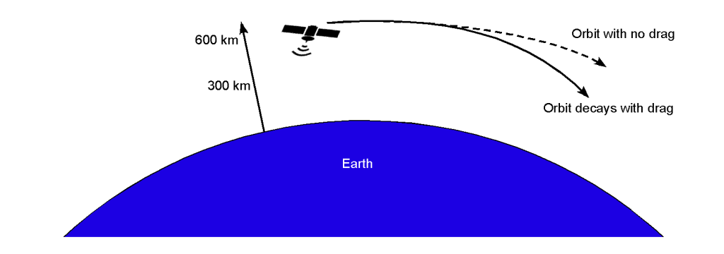
LEO is the region closest to Earth, extending from approximately 160 km to 2,000 km in altitude. Objects in LEO travel at very high velocities, typically around 7.8 km/s (17,500 mph), to maintain their orbits. Examples of objects in LEO include the International Space Station (ISS) and the Hubble Space Telescope (HST). Even at the high altitudes of LEO, the low atmospheric density exerts a drag force on satellites and other objects. This drag force causes a gradual loss of altitude, known as orbital decay. The drag force depends on the object’s velocity, cross-sectional area, and atmospheric density at the given altitude.
Orbital decay is a complex process influenced by several factors, including atmospheric density, which varies with altitude, solar activity, and the Earth’s rotation. During periods of high solar activity, the increased solar radiation heats the Earth’s atmosphere, causing it to expand and increase its density at higher altitudes. This results in greater drag on satellites. Semi-empirical models such as the Jacchia/Lineberry 1971 model are used to predict atmospheric density and, consequently, the drag force on objects in LEO. These models combine theoretical calculations with empirical data from satellite observations and other measurements. Satellites in LEO are equipped with thrusters to perform periodic boosts or reboost maneuvers to counteract the effects of drag and maintain their desired orbits. These maneuvers are essential for the operational lifespan of satellites, ensuring they remain in their designated orbits for as long as possible.
The International Space Station (ISS) orbits at an average altitude of about 400 km. Because of atmospheric drag, it loses about 2 km of altitude per month. Regular reboosts are performed to maintain its altitude and ensure continued operation. The Hubble Space Telescope (HST) orbits at an altitude of approximately 540 km. Although it experiences less drag than the ISS, it still requires occasional boosts to maintain its orbit.
Are there aerosol particles in the atmosphere?
Yes! An interesting fact about the atmosphere is that it contains tiny particles known as aerosols, which play a significant role in various atmospheric processes. Aerosols, including dust, pollen, volcanic ash, soot, and pollutants, can be natural or human-made. Despite their small size, aerosols can profoundly impact climate and weather patterns. They can scatter and absorb sunlight, affecting the amount of solar radiation reaching the Earth’s surface. This, in turn, can influence temperature patterns and the formation of clouds. Aerosols also play a crucial role in the formation of cloud droplets. They act as “seeds” around which water vapor can condense, forming tiny droplets that make up clouds. Without aerosols, clouds would not form as quickly or effectively.
Summary & Closure
When dealing with the performance of flight vehicles in the Earth’s atmosphere, it is essential to know (or estimate) the air density in which the vehicle is flying. The power and thrust from air-breathing powerplants are also affected by the air density in which they operate, and their performance generally diminishes with increasing altitude and/or temperature. To address these challenges, aeronautical engineers must have a deep understanding of the properties of the air in the troposphere and how these properties may impact the performance of their aircraft. They use this knowledge to make informed decisions about the design of the aircraft and to conduct tests to ensure that the aircraft meets its performance and safety requirements.
The International Standard Atmosphere (ISA) model forms a basis for standardization. The ISA is used universally in engineering and practical aviation, including as a basis for instrumentation calibration. The International Organization for Standardization (ISO) publishes the ISA model as ISO 2533:1975. The International Civil Aviation Organization (ICAO) has also adopted the ISA model, which is used universally throughout aviation. There are also various extended atmospheric models to represent the characteristics of the atmosphere above the tropopause and into space, which may be needed for multiple reasons, including estimates of the drag on satellites in low Earth orbit. It may also be necessary to know the properties of the atmospheres on other planets, such as for probes or landers.
5-Question Self-Assessment Quickquiz
For Further Thought or Discussion
- Program the ISA equations (use MATLAB or similar) and plot the temperature, pressure, and density as a function of altitude in U.S. customary (USC) units.
- Use the ISA tables to estimate air density at a pressure altitude of 5,500 ft where the temperature is 10F above standard. Confirm the result using the ISA equations.
- On a given day, the air temperature at 2,000 feet above mean sea level is 5C. What is this temperature value compared to the ISA temperature?
- In which atmospheric layer is most of the water vapor contained?
- Why does the temperature of the atmosphere increase with increasing altitude within the stratosphere?
Additional Online Resources
To improve your understanding of the atmosphere and the ISA, navigate to some of these online resources:
- High-definition video about the motion of the atmosphere.
- Take a ride on a U-2 spy-plane through the atmosphere to the edge of space.
- Try out this handy online ISA calculator.
- A lecture video on the ISA from Delft University.
- A YouTube video on the structure of the atmosphere for pilots.
- A good video summary of the ISA.
- UVB radiation has been linked to various harmful effects on human health and the environment. It contributes to global warming and is a significant risk factor for skin cancers such as melanoma. Additionally, excessive exposure to UVB radiation can lead to other human health issues, including cataracts and immune system suppression. ↵
- A hygrometer measures relative humidity as distinct from a hydrometer, which measures the specific gravity. Many kinds of analog and digital types are available. ↵
- Psychrometry is also called hygrometry, is a field that deals with gas-vapor mixtures. ↵
