Unsteady Aerodynamics, Aeroelasticity, & Flutter

J. Gordon Leishman

59 Unsteady Aerodynamics, Aeroelasticity, & Flutter

Introduction

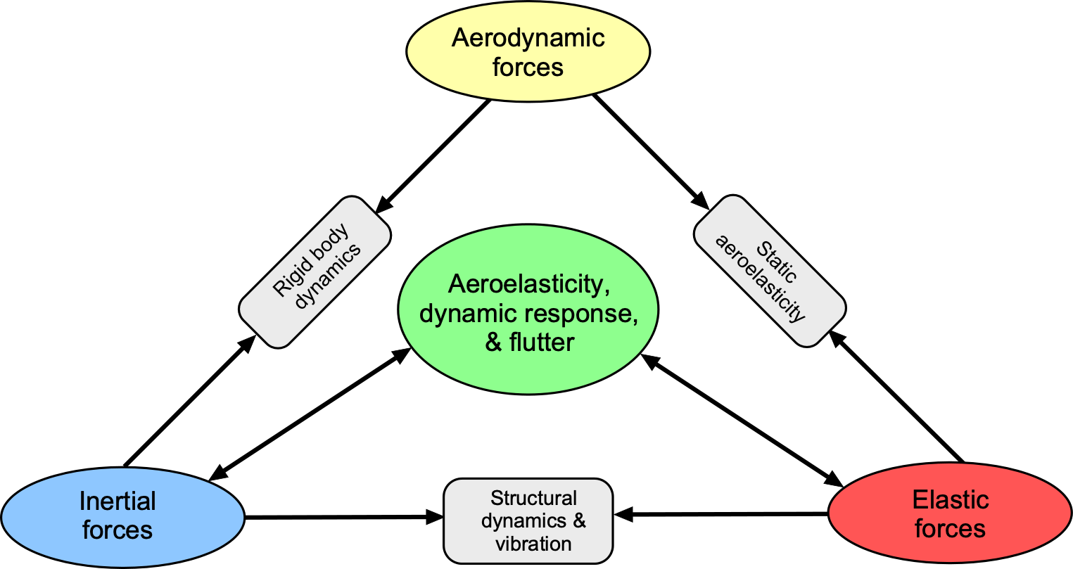
Aeroelasticity is a specialized field in aerospace engineering that examines the interactions between aerodynamic forces, elastic deformations, and the structural dynamics of aerospace structures. The essence of the field can be described by a Collar diagram^[1], which illustrates the interaction between the structural characteristics and the aerodynamic forces of a flight vehicle or another aeroelastic system. It helps understand a structure’s stability and dynamic behavior when subjected to aerodynamic loads. This video provides an overview of this fundamental behavior as it affects the wings and tails of different airplanes.

A Collar diagram shows the aeroelastic interplay between different energy components, including elastic, kinetic, and aerodynamic energy.

The origins of aeroelasticity date back to the early days of aviation, when unexpected wing failures occurred on the first monoplanes. Many of these failures were traced to a behavior that became known as aeroelastic divergence; as a critical airspeed was approached, the increase in aerodynamic forces caused a nose-up pitch twisting of the wing, as illustrated in the figure below. The consequence is excessively large pitch deformations and a further buildup of aerodynamic loads, so a catastrophic structural failure of the wing is inevitable unless airspeed is quickly reduced.

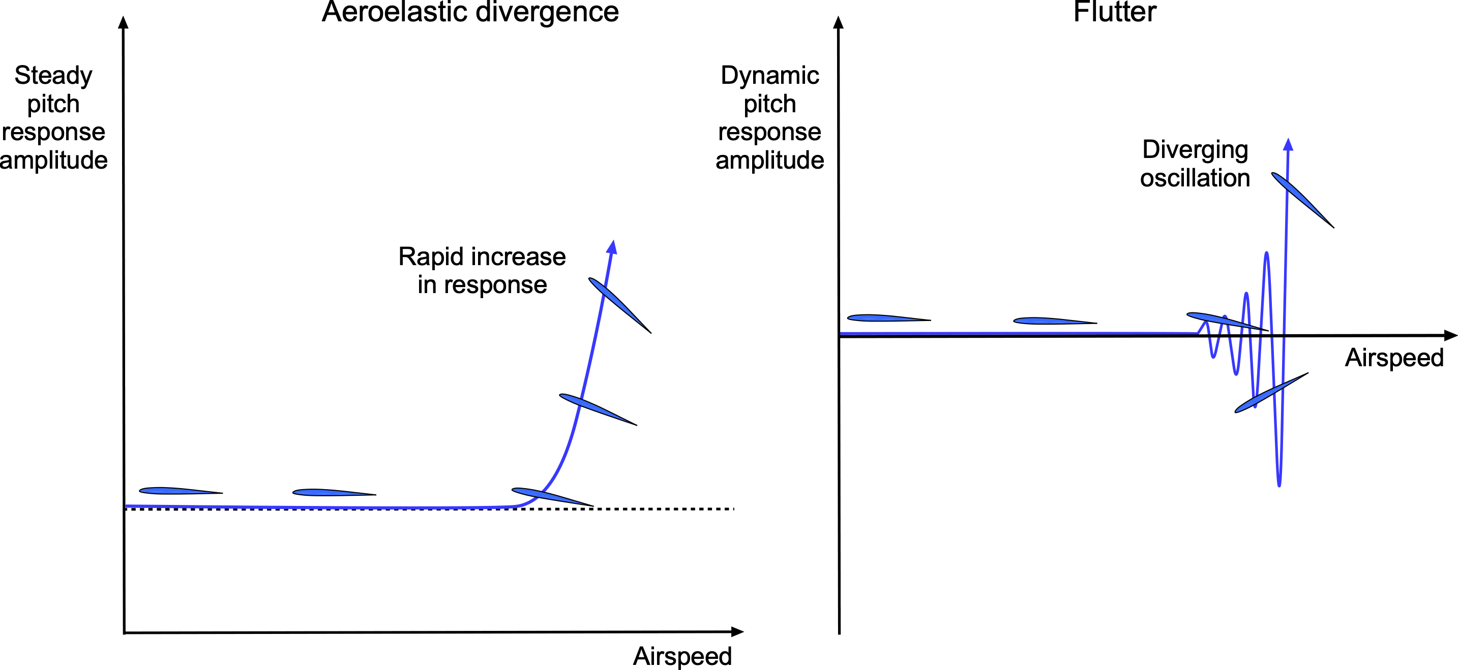
Aeroelastic effects can encompass but are not limited to phenomena such as structural divergence and flutter.

Flutter, another behavior that can lead to wing or tail surface failure, is a self-excited oscillation arising from the interplay between unsteady aerodynamic forces and the structure’s dynamic response. As shown in the figure above, flutter is an oscillatory response that can grow rapidly in amplitude as a critical airspeed is approached. At or near this critical airspeed, a minor disturbance, such as a gust or control input, can trigger the onset of flutter. The flutter can reach a limiting amplitude but can also become a divergent oscillatory response, i.e., a form of an aerodynamic/structural dynamic resonance. In these conditions, structural failure is also likely.

These observations and a history of structural failures with early airplanes revealed that structural elasticity and flutter avoidance could not be ignored during the design process. Understanding aeroelastic phenomena became even more critical with the development of higher-speed and supersonic airplanes, where aerodynamic forces and structural stresses were much more significant. Today, all aircraft must be designed for flutter-free operation over their entire flight envelopes, and thorough aeroelastic analyses and flight testing are integral to their design and certification process. This video from Airbus shows how engineers and pilots explore the flutter envelope of a new airplane.

Learning Objectives

Understand the basic principles of aeroelasticity and why it is crucial to designing and analyzing flight vehicles.
Explore unsteady aerodynamics and how it differs from steady-state aerodynamics.
Be able to apply Theodorsen’s theory to calculate unsteady lift, including apparent mass terms.
Learn about various aeroelastic phenomena, such as divergence, flutter, buffeting, and buzzing, and their relationships to steady and unsteady aerodynamic forces.
Appreciate how Computational Fluid Dynamics (CFD) and the Finite Element Method (FEM) can be more comprehensively used to model unsteady aerodynamics and flutter.

History

The origins of aeroelastic behavior can be traced back to the very first airplanes; see the review paper “Historical Development of Airplane Flutter” by I. E. Garrick and Wilmer H. Reed III. The Wright brothers and other early aviation pioneers sometimes encountered wing oscillations and various buzzing phenomena. They also noticed the buzzing effects on the tips of their propellers, which they solved by using blades with wider chords. They did not understand these effects back then, but they were likely of aeroelastic origin caused by the interaction of aerodynamic forces and structural dynamics. In 1902, Samuel Langley tried to fly an aircraft, but his monoplane’s wood and fabric wings were not stiff enough, and they twisted and broke off after a short flight, i.e., a form of aeroelastic divergence. The Wright brothers experimented with different structures and knew how to make a more rigid structure like a biplane, which did not suffer as readily from aeroelastic effects. The catastrophic failure of the horizontal tail on a Handley Page O/400 bomber in 1916 from an oscillatory aeroelastic phenomenon that was to become known as flutter suggested that much was still to be learned about aircraft design.

Wing and control surface flutter became an increasingly critical concern as aircraft designs evolved, particularly with the transition to monoplanes. Monoplanes, with their single-wing configuration and lower structural stiffness,^[2] highlighted the importance of understanding and mitigating flutter during aircraft design. “The Blue Max” is a 1966 film set in WWI that tells the story of a German fighter pilot, Bruno Stachel, who aims to earn the prestigious Pour le Mérite, also known as the “Blue Max,” for outstanding acts of bravery in aerial combat. While wing divergence and flutter are not a central theme in the movie, the film depicts the increased dangers of structural failure that early pilots faced when transitioning from flying slow biplanes to much faster and agile monoplanes.

The rapid advancement in aircraft design and increased flight speeds after this period led to more frequent and severe aeroelastic problems. Engineers then systematically studied these issues, formulating aeroelastic theories to predict and avoid flutter, which usually meant more rigorous structural design. The work of Theodore Theodorsen, among others, laid the groundwork for modern aeroelastic analyses. The severity of flutter issues in the decade following WW2 is underscored by a 1956 state-of-the-art survey conducted by the NACA Subcommittee on Vibration and Flutter, which documented 54 instances of flutter-related difficulties with U.S. military aircraft. The introduction of thin swept wings for supersonic flight in the 1950s increased the challenges of predicting aeroelastic effects at higher Mach numbers. This period saw significant advancements in theoretical, wind tunnel, and flight testing, including a better understanding of unsteady aerodynamic effects.

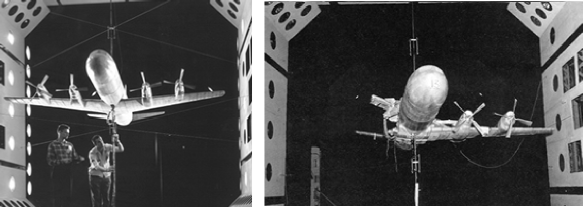
The Lockheed L-188 Electra, a four-engine turboprop airliner introduced in the late 1950s, was found to suffer from a more complicated but catastrophic type of flutter called whirl mode flutter. Under some conditions, propeller oscillations were transmitted as forces to the engine mountings, which coupled to the wings and created dangerous vibrations. After two midair breakups where the wings broke off the airplane, design changes included reinforced engine mounts and thicker wing skins, making the airplane flutter-free. While these failures damaged the reputation of the airplane and its manufacturer, the modified Electra became a reliable aircraft, the P-3 Orion being used extensively by the U.S. Navy until quite recently. While flutter prediction methods continued to advance, wind tunnel testing of aeroelastic Froude-scaled models remained crucial for validating predictive methods. Steps were also taken to establish formal criteria for predicting and mitigating the onset of flutter before the aircraft’s first flight.

A 1/8th-scale powered model of the Electra was tested in the NASA Langley 19-foot tunnel. It proved that the crashes occurred because of a phenomenon known as a whirl flutter, which caused catastrophic wing failure.

The development of supersonic airplanes, including military (e.g., SR-71) and civil (e.g., Concorde), as well as hypersonic vehicles encountering thermal heating (e.g., the X-15), further pushed the boundaries of aeroelastic research. More comprehensive computational methods emerged during the 1980s, allowing for more confident predictions of aeroelastic effects and flutter. Today, computational tools such as Computational Fluid Dynamics (CFD) and the Finite Element Method (FEM), which can be coupled to include structural dynamics, are integral to most forms of comprehensive aeroelastic analysis. These methods allow for accurate simulations of aeroelastic interactions between airframe components, particularly for complex geometries and high-speed flight conditions. Unlike analytical solutions, which are more limited, CFD and FEM integration enables engineers to analyze the full spectrum of aeroelastic behavior for an entire flight vehicle, including wings, control surfaces, engines, undercarriage, and other components. Aeroelasticity is not just a concern for airplanes because it plays a crucial role in the design of helicopter rotors, wind turbines, and even bridges.

As flight speeds continue to increase and airplane construction evolves toward even lighter and more flexible aerostructures, understanding and controlling aeroelastic effects remain an ongoing engineering challenge. Using active control, either structural or aerodynamic, or both, can help mitigate undesirable aeroelastic effects with lightweight structures. For example, the Boeing 787 has a Flaps-Up Vertical Modal Suppression (F0VMS) system ^[3] to enhance the damping of a stable but lightly-damped low-frequency aeroelastic mode between the engines, wings, and fuselage. This system, which uses differential elevator inputs and flaperons, is designed to produce damping augmentation, not flutter suppression; the FAA does not currently approve active flutter suppression systems for operational use.

Unsteady Airfoil Behavior

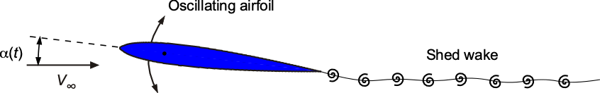
Fundamental to the prediction of flutter is the modeling of unsteady aerodynamics. Unsteady airfoil theory deals with the aerodynamic behavior of airfoils and wings when subjected to time-varying boundary conditions, such as oscillations in the angle of attack, vertical and horizontal motions, or other conditions where the angle of attack may change with respect to time.

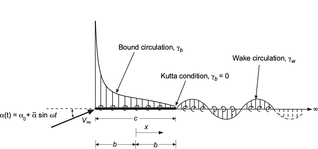
In an unsteady flow, the wake behind the airfoil is time-varying in structure with the shedding of vorticity and circulation, as shown in the figure below, thereby influencing the aerodynamic forces experienced by the airfoil. These wake effects change the magnitude of the lift and the phase of the lift response relative to the time-varying boundary conditions. Furthermore, at high angles of attack, the flow may separate from the airfoil surface, causing leading edge vortex shedding and aerodynamic hysteresis, a phenomenon called dynamic stall. Under these conditions, the reduced aerodynamic damping can produce another form of flutter called stall flutter.

When the angle of attack changes, the immediate downstream shed wake affects the aerodynamics of the airfoil section.

There are many ways to calculate these unsteady effects quantitatively. One instructive approach for those first learning about unsteady airfoil behavior is the classic linearized unsteady aerodynamics theories, including Theodorsen’s theory and the indicial response method. Unsteady panel methods discretize the airfoil surface into panels extending into the wake, capturing the same physical phenomena. The most computationally intensive CFD methods solve the Navier-Stokes equations for unsteady flow, which can capture detailed flow phenomena, including the wake, vortex shedding, and dynamic stall, although at significant computational cost and time.

Reduced Frequency

A nondimensional parameter used to help categorize whether a flow is steady or unsteady is the reduced frequency, given the symbol $k$ . The reduced frequency is defined, in general, as

(1) $\begin{equation*} k = \frac{\omega \, L}{V} \end{equation*}$

where $\omega$ is a characteristic physical frequency of the unsteady flow (in units of radians per second), $L$ is a characteristic length scale, and $V$ is a reference flow velocity. Base units should always be used to obtain the correct numerical value for the reduced frequency.

For a wing or airfoil, such as one oscillating in angle of attack or an oscillatory vertical (heaving) motion as shown in the figure below, the reduced frequency is often defined in terms of its semi-chord, i.e., $L = c/2 = b$ , and the free-stream velocity, $V_{\infty}$ , i.e., in this case, it is defined as

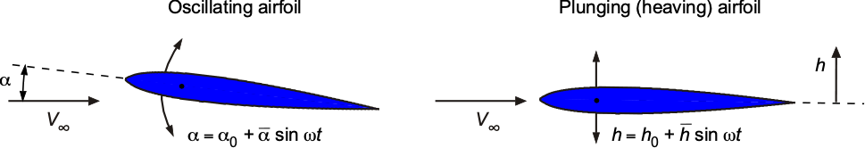
(2) $\begin{equation*} k = \frac{\omega \, c}{2 \, V_{\infty}} = \frac{\omega \, b}{V_{\infty}} \end{equation*}$

Unsteady airfoil motion produces different aerodynamic characteristics than a steady flow; these issues are encountered in aeroelasticity.

The aerodynamics of non-steady and oscillating airfoil sections and wings must be addressed in the field of aeroelasticity and flutter. For example, a torsional wing motion introduces a pitching behavior at any wing section, as shown in the figure above. Likewise, a bending motion of the wing introduces a plunging or heaving behavior at the wing section. Both types of motion will change the effective angle of attack and contribute to the aerodynamic loads, with increasing reduced frequencies causing more significant aerodynamic effects.

For $k$ = 0, the flow is steady, and all the usual steady results will apply regarding the relationships between the aerodynamic quantities and the angle of attack. For 0 $\le k \le$ 0.05, the flow can be considered quasi-steady; that is, unsteady effects are generally minor, and for some problems, they may be neglected completely. Under these conditions, the aerodynamic response is related to the instantaneous forcing conditions, i.e., no significant time-history effect exists. Nevertheless, as will be explained, additional quasi-steady “apparent mass” aerodynamic terms related to the airfoil section’s velocities and accelerations will need to be included, which may begin to affect both the amplitude and phase of the aerodynamic response.

Flows with characteristic reduced frequencies of 0.05 and above are typically considered as unsteady, so all unsteady terms must be retained in the governing flow equations, including the effects of the shed wake. The manifestation of this is more significant changes in amplitude and phase response of the aerodynamic loads with respect to the motion, which are frequency dependent. Such aerodynamic and aeroelastic problems are more challenging to model for two reasons. First, the local flow properties also depend on the previous time, i.e., what has happened in the time history of the lift and other aerodynamic forces. Second, the effects of compressibility may need to be included even if the free-stream flow velocity is low, which introduces additional challenges in modeling the unsteady aerodynamic response.

Quasi-Steady Aerodynamics

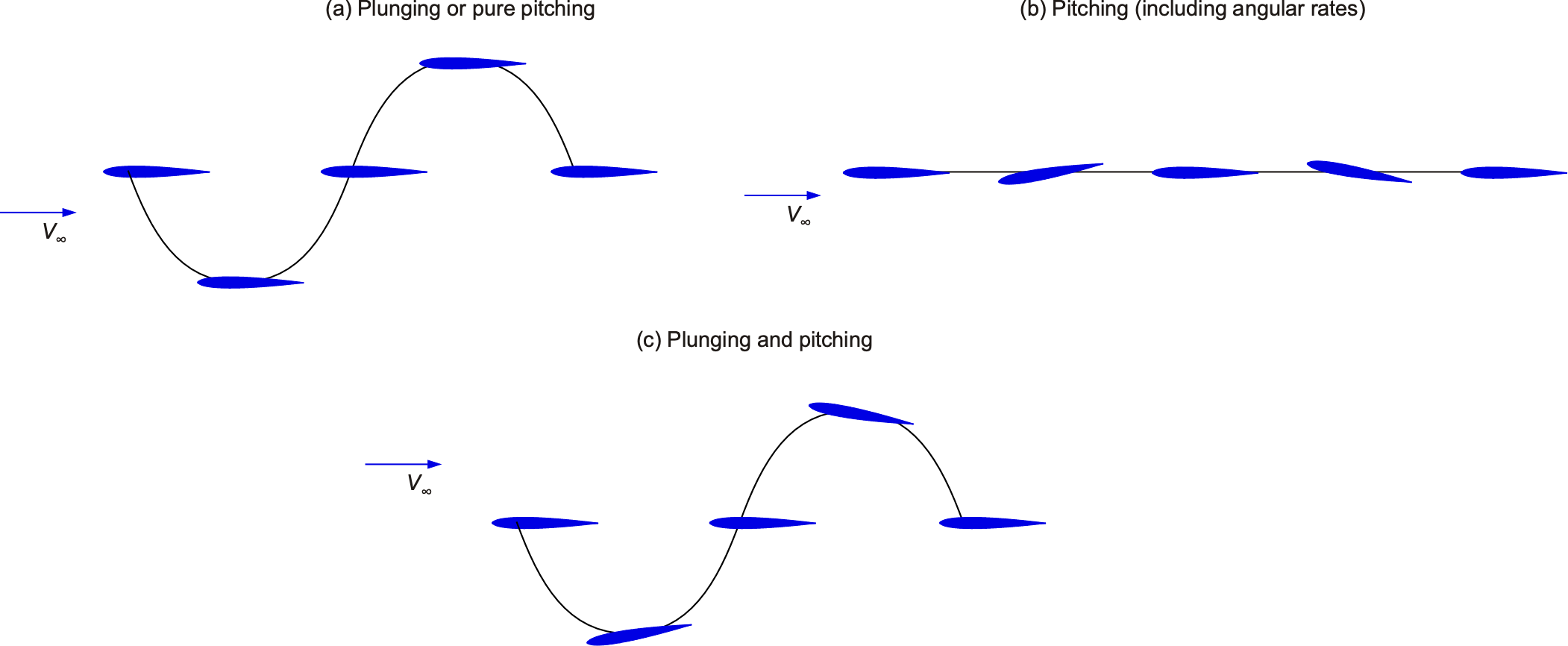
In quasi-steady aerodynamics, the behavior can be evaluated by applying the principles of steady flow under the instantaneous boundary conditions of flow tangency to the airfoil surface. Different forcing conditions, such as pure plunge or pitch, pitching, and a combination of pitching and plunging, may be considered, as shown in the figure below.

At the wing sectional level, displacements can comprise pure plunge or pitch, pitching, and a combination of pitching and plunging.

For example, for a thin airfoil,^[4]the changes in the angle of attack of a harmonically oscillating airfoil can be expressed as

(3) $\begin{equation*} \alpha (t) = \alpha_0 + \bar{\alpha} \sin \omega t \end{equation*}$

where $\alpha_0$ is the mean angle of attack and $\bar{\alpha}$ is the angle of attack amplitude of the oscillation. If the flow were quasi-steady, in the sense that flow adjustments were to take place instantaneously, the circulatory part of the lift coefficient would be given by

(4) $\begin{equation*} C_l (t) = C_{l_{\alpha}} \left( \alpha + \frac{\overbigdot{\alpha} \, c}{2 \, V_{\infty}} \right) \end{equation*}$

recognizing that the pitch rate, i.e., $\overbigdot{\alpha}$ , must affect the lift coefficient because it changes the angle of attack. This equation then leads to

(5) $\begin{equation*} C_l (t) = C_{l_{\alpha}} \bigg( \alpha_0 + \bar{\alpha} \sin \omega t + k \, \bar{\alpha} \cos \omega t \bigg) = C_{l_{\alpha}} \sqrt{1 + k^2} \bigg( \alpha_0 + \bar{\alpha} \sin (\omega t + \phi ) \bigg) \end{equation*}$

where $\phi$ is a frequency-dependent phase angle given by

(6) $\begin{equation*} \phi = \tan^{-1} \big( k \big) \end{equation*}$

Therefore, even based on quasi-steady arguments, the circulatory part of the lift response will no longer be in phase with the angle of attack (it will lead by the angle $\phi$ in this case) nor have the same amplitude (it is larger than $C_{l_{\alpha}}$ by a factor $\sqrt{1 + k^2}$ ).

Notice that because the aerodynamic center is at the 1/4 chord for a thin airfoil, then $C_{m_{1/4}} = 0$ for the circulatory parts of the quasi-steady aerodynamic response.

Apparent Mass Terms

The apparent mass or “noncirculatory” terms^[5] account for the pressure forces required to accelerate the fluid near the airfoil. For example, consider a thin airfoil of chord $c$ moving normal to its surface at velocity $w(t)$ , the noncirculatory fluid force, $F_{\rm nc}$ , acting on the surface is

(7) $\begin{equation*}F_{\rm nc} = -{\cal{M}}_a \, \frac{dw}{dt} \end{equation*}$

The term ${\cal{M}}_a$ is often known as the apparent mass or added mass, and in this case is given by

(8) $\begin{equation*} {\cal{M}}_a = \pi \varrho \, \frac{c^2}{4} \end{equation*}$

Therefore, the noncirculatory lift (per unit span) for a motion where the airfoil moves normal to its surface with velocity $w = \overbigdot{h}$ , as shown in the figure below, is

(9) $\begin{equation*} L'_{\rm nc} = \pi \varrho \, \dfrac{c^2}{4} \overbigddot{h} \end{equation*}$

Noncirculatory or “apparent mass” terms are related to the airfoil section’s instantaneous translational and angular accelerations.

In terms of lift coefficient, then

(10) $\begin{equation*} C_{l_{\rm nc}} = \left( \dfrac{\pi \varrho \, \dfrac{c^2}{4}}{\dfrac{1}{2} \varrho \, V_{\infty}^2 \, c} \right) \overbigddot{h} = \left( \frac{\pi \, b}{V_{\infty}^2} \right) \overbigddot{h} \end{equation*}$

As shown in the figure above, an additional moment contribution arises from the rotational acceleration when the airfoil undergoes a pitching motion about any axis. For example, and simplicity, consider the pitch rate about the leading edge, $\overbigdot{\theta}$ , then the noncirculatory lift force is

(11) $\begin{equation*} L'_{\rm nc, \, \overbigdot{\theta}} = -\frac{\pi}{8} \varrho \, c^3 \overbigddot{\theta} \end{equation*}$

In terms of lift coefficient, then

(12) $\begin{equation*} C_{l_{\rm nc, \, \overbigdot{\theta}}} = -\frac{\pi}{4} \left( \frac{c}{V_{\infty}^2} \right) \overbigddot{\theta} = -\left( \frac{\pi c}{4 V_{\infty}^2} \right) \overbigddot{\theta} \end{equation*}$

Therefore, the total noncirculatory lift contribution from a combination of pitch and plunge will be

(13) $\begin{equation*} C_{l_{\rm nc}} = \left( \frac{\pi b}{V_{\infty}^2} \right) \overbigddot{h} - \left( \frac{\pi c}{4 V_{\infty}^2} \right) \overbigddot{\theta} \end{equation*}$

The corresponding moment about the leading edge from pitch rate is

(14) $\begin{equation*} M'_{\rm nc, \, LE} = -\dfrac{\pi}{8} \varrho \, c^3 \, \overbigddot{\theta} \end{equation*}$

In terms of the moment coefficient, then

(15) $\begin{equation*} C_{m_{\rm nc, \, LE}} = - \left( \frac{\dfrac{\pi}{8} \varrho \, c^3}{\dfrac{1}{2} \varrho \, V_{\infty}^2 c^2} \right) \overbigddot{\theta} = -\left( \frac{\pi \, c}{4 \, V_{\infty}^2} \right) \overbigddot{\theta} \end{equation*}$

The moment about the 1/4-chord is related to the leading-edge moment by the application of statics using

(16) $\begin{equation*} C_{m_{\rm nc, \, 1/4}} = C_{m_{\rm nc, \, LE}} + \left( \frac{1}{4} \right) C_{l_{\rm nc}} \end{equation*}$

Therefore, it is apparent that incorporating the apparent mass or noncirculatory effects introduces additional terms that are proportional to the airfoil’s acceleration, including translation (plunge), i.e., \overbigddot{h} and rotation (pitch), i.e., $\overbigddot{\theta}$ . Unlike the circulatory air loads, which depend on the instantaneous angle of attack and its rate of change, the noncirculatory forces depend directly on acceleration. These effects are most pronounced in high-frequency oscillations where $\overbigddot{h}$ and $\overbigddot{\alpha}$ are large. They are also essential for predicting unsteady airloads in transient motions, such as airplanes undergoing quick pitch-up maneuvers.

Quasi-Steady Aerodynamics, Including Apparent Mass

Using the previous oscillatory motion example, the noncirculatory contribution to the lift is given by

(17) $\begin{equation*} C_{l_{\text{nc}}} (t) = \left( \frac{\pi \, c}{2 V_{\infty}} \right) \overbigddot{\alpha} \end{equation*}$

Adding this term to the previous circulatory lift expression gives

(18) $\begin{equation*} C_l (t) = C_{l_{\alpha}} \left( \alpha + \frac{\overbigdot{\alpha} \, c}{2 V_{\infty}} \right) + \left( \frac{\pi \, c}{2 V_{\infty}} \right) \overbigddot{\alpha} \end{equation*}$

Substituting $\alpha (t) = \alpha_0 + \bar{\alpha} \sin \omega t$ leads to $\overbigdot{\alpha} = \omega \bar{\alpha} \cos \omega t$ and $\overbigddot{\alpha} = -\omega^2 \bar{\alpha} \sin \omega t$ . Therefore, the total lift coefficient is

(19) $\begin{equation*} C_l (t) = C_{l_{\alpha}} \left( \alpha_0 + \bar{\alpha} \sin \omega t + k \bar{\alpha} \cos \omega t \right) - \pi k^2 \bar{\alpha} \sin \omega t \end{equation*}$

which, after some rearrangement, becomes

(20) $\begin{equation*} = C_{l_{\alpha}} \sqrt{k^2 + \left(1 - \frac{\pi k^2}{C_{l_{\alpha}}} \right)^2} \, \, \bigg( \alpha_0 + \bar{\alpha} \sin (\omega t + \phi') \bigg), \quad \text{where} \quad \phi' = \tan^{-1} \left( \frac{k}{1 - \dfrac{\pi k^2}{C_{l_{\alpha}}}} \right) \end{equation*}$

These results show that the apparent mass effect modifies the amplitude and gives a phase shift of the lift response, depending on the value of the reduced frequency. The upshot of this is that the aerodynamic forces will have different values depending on whether the angle of attack is increasing or decreasing with respect to time. Indeed, measurements suggest that the unsteady lift on an airfoil or wing is often attenuated (diminished) by unsteady effects and not amplified as the quasi-steady theory would suggest. Still, there can be a lag or a lead in the aerodynamic response with respect to the angle of attack.

Frequency Domain – Theodorsen’s Theory

Although extensive literature exists, accounting for the unsteady “shed wake” effects adds significant mathematical complexity to developing an unsteady airfoil theory. One of these theories is called Theodorsen’s theory. Theodorsen’s theory^[6] provides a linearized, small-disturbance solution for oscillating airfoils in an incompressible flow. The theory is based on the assumption of small oscillation amplitudes. It gives an exact analytic theory (within the stated assumptions and limitations of thin airfoil theory) to describe the unsteady airloads on a thin airfoil. Theodorsen’s problem was obtaining the solution for the loading (bound circulation) $\gamma_b$ on the airfoil surface under harmonic forcing conditions, the flow model being shown in the figure below.

Flow model used for Theordorsen’s theory. The objective is to find the unsteady loading on a thin airfoil accounting for the effects of circulation shed into the downstream wake.

Governing Equation

The governing integral equation is

(21) $\begin{equation*} w(x,t) = \frac{1}{2\pi} \int_0^c \frac{\gamma_b(x,t)}{(x-x_0)} dx + \frac{1}{2\pi}\int_c^{\infty} \frac{\gamma_w(x,t)}{(x-x_0)} dx \end{equation*}$

where $w$ is the downwash on the airfoil surface. This equation must be solved subject to flow tangency on the airfoil chord and by invoking the Kutta condition at the trailing edge, i.e., $\gamma_b (c,t) = 0$ . There is also a connection to be drawn between the change in circulation about the airfoil and the circulation shed into the wake. Conservation of circulation (Kelvin’s theorem) requires that

(22) $\begin{equation*} \gamma_w(c,t) dx = -\frac{d\Gamma(t)}{dt} dt \end{equation*}$

Assuming that the vorticity in the shed wake is convected at the free stream velocity, $V_{\infty}$ , this gives $dx = V_{\infty} dt$ , and so

(23) $\begin{equation*} V_{\infty} \gamma_w(c,t) = -\frac{d\Gamma(t)}{dt} \end{equation*}$

where the total circulation about the airfoil, $\Gamma(t)$ is given by

(24) $\begin{equation*} \Gamma(t) = \int_0^c \gamma_b(x,t) dx \end{equation*}$

Because this wake vorticity is close to the airfoil, it changes the downwash velocity, so the loads on the airfoil are also affected. Suppose the net circulation about the airfoil is changing harmonically with respect to time, as in Theodoresen’s problem. In that case, circulation will be harmonically shed into the wake and continuously affect the airfoil’s aerodynamic loads. In the limit, as the changing boundary conditions end, the shed wake vorticity cast off the trailing edge of the airfoil becomes zero, and the remaining circulation in the wake convects downstream to infinity, thereby recovering the classic thin airfoil theory.

Theodorsen Function

The unsteady problem posed above is certainly not trivial to solve. Still, for a simple harmonic motion, the solution is given by Theodorsen in a form that represents a transfer function between the forcing (angle of attack) and the aerodynamic response (i.e., the chordwise loading distribution, lift, and pitching moment). The solution, which is given in terms of the Theodorsen function, denoted by $C(k)$ , is a complex-valued function that captures the instantaneous effect of the circulation shed into the wake on the unsteady aerodynamic response and is given by

(25) $\begin{equation*} C(k) = F(k) + i G(k) = \frac{H_1^{(2)}(k)}{H_1^{(2)}(k) + i H_0^{(2)}(k)} \end{equation*}$

where $H_0^{(2)}$ and $H_1^{(2)}$ are Hankel functions of the second kind, and $k$ is the reduced frequency. The Hankel function is defined as $H_{\rm v}^{(2)} = J_{\rm v} - i Y_{\rm v}$ , with $J_{\rm v}$ and $Y_{\rm v}$ being Bessel functions of the first and second kind, respectively. Therefore, the $C(k)$ function can be viewed as an aerodynamic transfer function that relates the input (forcing) to the response.

Recognizing that each Bessel function has an argument $k$ , then the real or in-phase ( $\Re$ ) part and imaginary or out-of-phase part ( $\Im$ ) of the Theodorsen function can be written as

(26) $\begin{equation*} \Re C(k) = F = \frac{J_1 ( J_1 + Y_0 ) + Y_1 (Y_1 - J_0)}{(J_1 + Y_0)^2 + (J_0 - Y_1)^2} \end{equation*}$

and

(27) $\begin{equation*} \Im C(k) = G = -\frac{Y_1 Y_0 + J_1 J_0}{(J_1 + Y_0)^2 + (J_0 - Y_1)^2} \end{equation*}$

Despite its apparent mathematical complexity, the Theodorsen function is readily calculated numerically using MATLAB and is plotted in the figure below.

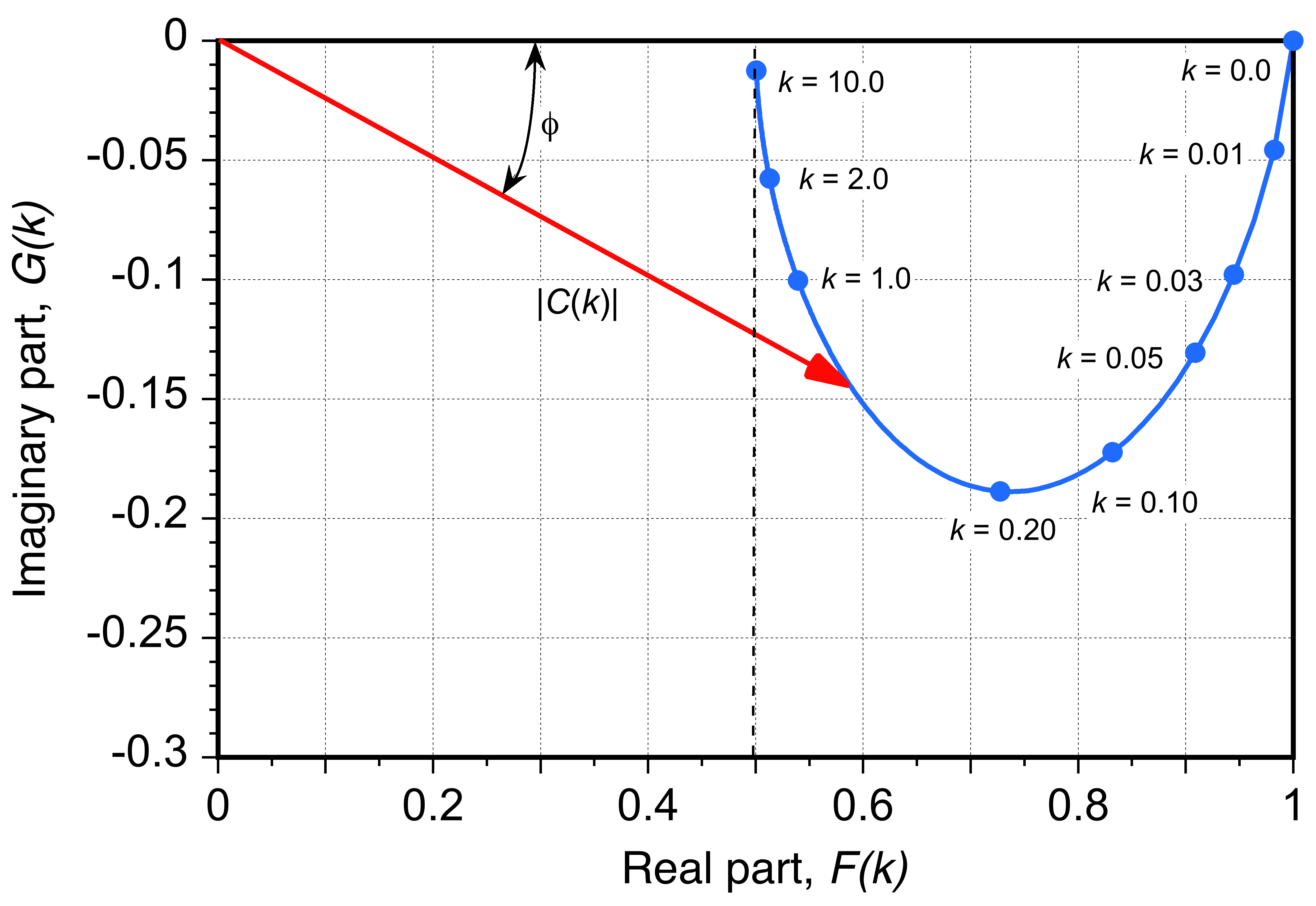
Theodorsen’s function plotted in terms of its real and imaginary parts.

Another way of interpreting the Theodorsen function, which is perhaps more tangible in the first instance, is in terms of the amplitude, $| C(k) |$ , and phase angle, $\phi$ , of the response, which are given by

(28) $\begin{equation*} | C(k)| = \sqrt{ F^2 + G^2} \quad \mbox{and} \quad \phi = \tan^{-1} \left( \frac{G}{F} \right) \end{equation*}$

MATLAB code to calculate the Theodorsen function

Show the code/hide the code.

function theodorsen_function_plot_and_save
% Define the range of reduced frequencies
k = linspace(0.01, 10, 500); % Example range from 0.01 to 10 with 500 points

% Preallocate arrays for real and imaginary parts
Ck_real = zeros(size(k));
Ck_imag = zeros(size(k));

% Calculate the Theodorsen function for each k
for i = 1:length(k)
[Ck_real(i), Ck_imag(i)] = theodorsen_function(k(i));
end

% Plot the real part
figure;
subplot(2, 1, 1);
plot(k, Ck_real, ‘b-‘, ‘LineWidth’, 1.5);
xlabel(‘Reduced Frequency k’);
ylabel(‘Real Part of C(k)’);
title(‘Real Part of Theodorsen Function’);
grid on;

% Plot the imaginary part
subplot(2, 1, 2);
plot(k, Ck_imag, ‘r-‘, ‘LineWidth’, 1.5);
xlabel(‘Reduced Frequency k’);
label(‘Imaginary Part of C(k)’);
title(‘Imaginary Part of Theodorsen Function’);
grid on;

% Save the data to a file
data = [k.’, Ck_real.’, Ck_imag.’];
save(‘theodorsen_function_data.txt’, ‘data’, ‘-ASCII’, ‘-double’);
end

function [Ck_real, Ck_imag] = theodorsen_function(k)
% This function calculates the Theodorsen function C(k)
% and returns its real and imaginary parts.
% k is the reduced frequency

% Bessel functions of the first kind
J0 = besselj(0, k);
J1 = besselj(1, k);

% Bessel functions of the second kind
Y0 = bessely(0, k);
Y1 = bessely(1, k);

% Hankel functions of the second kind
H1 = J1 – 1i * Y1;
H0 = J0 – 1i * Y0;

% Theodorsen function C(k)
Ck = H1 ./ (H1 + 1i * H0);

% Separate into real and imaginary parts
Ck_real = real(Ck);
Ck_imag = imag(Ck);
end

It will be apparent that Theodoresen’s theory is a frequency domain theory; even though the results for the aerodynamic response may be expressed as a function of time, the unsteady forcing must be oscillatory, which is expressed in terms of the reduced frequency. Recall that the reduced frequency is a dimensionless parameter representing the unsteadiness of the flow, defined by

(29) $\begin{equation*} k = \frac{\omega c}{2\, V_\infty} \end{equation*}$

Physically, the reduced frequency can be interpreted as the ratio of the oscillation frequency to the convective frequency of the flow. Airfoils respond differently to different values of $k$ . Low $k$ values imply a quasi-steady behavior, while high $k$ values indicate highly unsteady conditions. Quasi-steady means that the flow responds almost immediately to any changes in the angle of attack; therefore, the aerodynamic response will be in phase with the airfoil motion.

Aerodynamic Response

The effect of the Theodorsen function, which emulates a physical wake lag response, can be appreciated if a pure oscillatory variation in the angle of attack is considered, as before, i.e., $\alpha (t) = \alpha_0 + \bar{\alpha} \sin \omega t$ ,^[7] where $\alpha_0$ is the mean angle of attack and $\bar{\alpha}$ is the angle of attack amplitude of the oscillation. If the flow were quasi-steady, in the sense that flow adjustments were to take place instantaneously, the lift coefficient would be given by

(30) $\begin{equation*} C_l (t) = C_{l_{\alpha}} \alpha = C_{l_{\alpha}} \left( \alpha_0 + \bar{\alpha} \sin \omega t \right) \end{equation*}$

where $C_{l_{\alpha}} = 2 \pi$ for a thin-airfoil in incompressible flow. In the unsteady case, this circulatory part of the airfoil lift coefficient becomes

(31) $\begin{equation*} C_l(t) = C_{l_{\alpha}}| C(k)| \bigg( \alpha_0 + \bar{\alpha} \sin ( \omega t + \phi ) \bigg) \end{equation*}$

or in terms of the real and imaginary parts, then

(32) $\begin{equation*} \Re C_l(t) = C_{l_{\alpha}} \left( \alpha_0 + \bar{\alpha} \sin \omega t \right) \, F(k)\quad \mbox{and} \quad \Im C_l(t) = C_{l_{\alpha}} \left( \alpha_0 + \bar{\alpha} \sin \omega t \right) \, G(k) \end{equation*}$

The amplitude and phase lag of the lift response is then

(33) $\begin{equation*} | C_l(t)| \sqrt{ \Re C_l^2 + \Im C_l^2 }\quad \mbox{and} \quad \phi = \tan^{-1} \left( \dfrac{\Im C_l}{\Re C_l} \right) \end{equation*}$

Representative results from the Theodorsen theory are shown in the figure below in terms of lift coefficient $C_l$ versus angle of attack, $\alpha$ . Notice that the Theodorsen function introduces an amplitude reduction and phase lag effect on the circulatory part of the lift response compared to the result obtained under quasi-steady conditions.

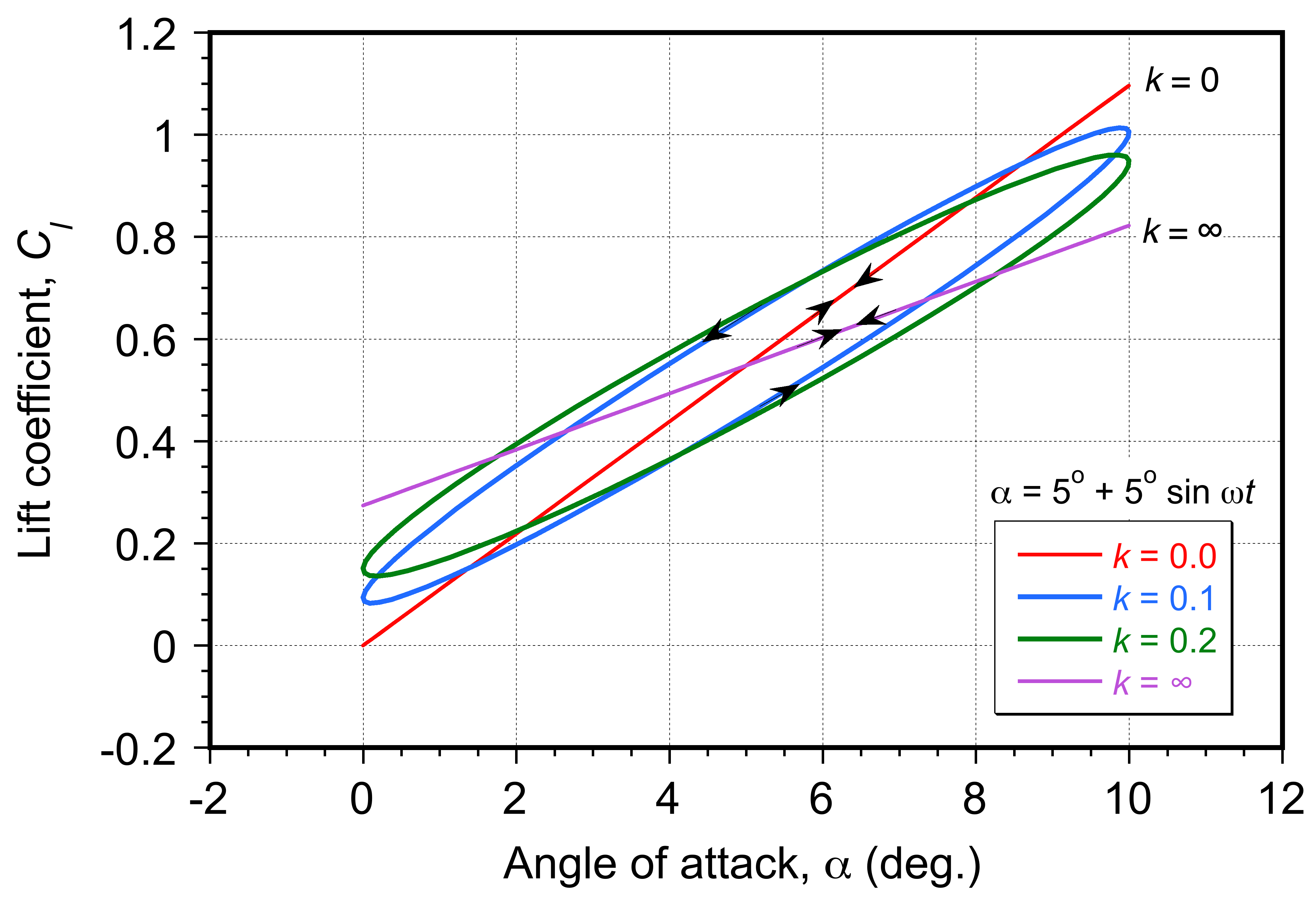
Representative unsteady lift coefficient versus angle of attack on an airfoil when oscillating at different reduced frequencies.

For $k = 0$ , the steady-state lift behavior is obtained, i.e., $C_l$ is linearly proportional to $\alpha$ . However, as $k$ is increased, the lift plots develop into hysteresis loops, and these loops rotate such that the amplitude of the lift response (slope of the lift curve) decreases with increasing values of reduced frequency. Notice also that these loops are circumvented in a counterclockwise direction such that the lift is lower than the steady value when $\alpha$ is increasing with time and higher than the steady value when $\alpha$ is decreasing with time, i.e., there is a phase lag accounted for by $\phi$ . Notice also that for infinite reduced frequency, the circulatory part of the lift amplitude is half that at $k=0$ , and there is no phase lag angle.

These concepts are readily extended to more complicated boundary conditions, including the effects of pitch rate and combinations of frequencies. Because the method is fundamentally a potential flow solution, linear superposition can be used to obtain the results for a more general forcing, such as a Fourier series.

Worked Example #1

An airfoil is undergoing harmonic pitching motion about its quarter-chord in a freestream with velocity $V_{\infty} = 50$ m/s. The pitching motion is described as $\theta(t) = \theta_0 \, e^{i\omega t}$ where the amplitude of motion is $\theta_0 = 5^\circ$ , and the oscillation frequency is $\omega = 10$ rad/s. The airfoil has a chord length of $c = 1$ m. Using Theodorsen’s theory, compute the unsteady lift coefficient, including its magnitude and phase angle.

Show solution/hide solution.

The reduced frequency is given by

$k = \frac{\omega c}{2V_{\infty}} = \frac{10 \times 1}{2 \times 50} = 0.1$

From Theodorsen’s function for $k = 0.1$ , then

$C(0.1) \approx 0.94 - 0.07i$

The effective angle of attack is

$\alpha(t) = \theta(t) + \frac{\overbigdot{\theta}(t) c}{2 V_{\infty}}$

Using Theodorsen’s equation for the unsteady lift coefficient:

$C_l = 2\pi C(k) \alpha(t)$

Substituting $\theta_0 = 5^\circ = 0.0873$ rad, $\theta(t) = \theta_0 \, e^{i\omega t}$ , and $\overbigdot{\theta}(t) = i\omega \theta_0 \, e^{i\omega t}$ , then

$C_l = 2\pi (0.94 - 0.07i) \left( 0.0873 + i k \times 0.0873 \right) \, e^{i\omega t} = 2\pi (0.94 - 0.07i)(1 + 0.1i) \times 0.0873 \, e^{i\omega t}$

Therefore,

$C_l = 2\pi \times 0.0873 \times (0.933 + 0.024i) \, e^{i\omega t} = 0.511 \, e^{i(\omega t + 1.47^\circ)}$

This represents an attenuation of the lift amplitude compared to the quasi-steady result, plus a small phase lead of $1.47^{\circ}$ , primarily because of the phase lead contributed by the pitch rate term.

It should also be appreciated that Theodorsen’s theory applies only to the “circulatory” component of the lift, i.e., the aerodynamic response associated with the creation and shedding of circulation. Additional non-circulatory forces (and moments) are produced by inertial effects or “apparent mass” in an unsteady flow. These effects must be included to round out the unsteady aerodynamic theory if it is to be used in any predictive sense.

Worked Example #2

Using conditions in Worked Example #2, determine the total unsteady lift coefficient, including Theodorsen’s circulatory and non-circulatory (added mass) lift components.

Show solution/hide solution.

The non-circulatory (apparent mass) lift coefficient for this motion is

$C_{l_{\rm nc}} = \pi \frac{c}{2V_{\infty}} \overbigddot{\theta}(t)$

Because $\overbigddot{\theta}(t) = -\omega^2 \theta_0 \, e^{i\omega t}$ , then

$C_{l_{\rm nc}} = -\pi \frac{ \omega^2 c}{2V_{\infty}}\theta_0 \, e^{i\omega t}$

Substituting $\dfrac{c}{2V_{\infty}} = \dfrac{1}{100}$ and $\omega = 10$ , gives

$C_{l_{\rm nc}}= -\pi \times \frac{1}{100} \times 10^2 \times 0.0873 \, e^{i\omega t} = -\pi \times 0.0873 \, e^{i\omega t} = -0.274 \, e^{i\omega t}$

which is a 180 $^{\circ}$ phase lead. Summing the circulatory and non-circulatory contributions gives

$C_l = C_{l_{c}} + C_{l_{\rm nc}} = (0.511 - 0.274) \, e^{i(\omega t + 1.47^\circ)} = 0.237 \, e^{i(\omega t + 1.47^\circ)}$

Time-Domain – The Indicial Response

The indicial aerodynamic response method provides a time-domain framework to calculate unsteady aerodynamic forces and moments in the time domain. Indicial response refers to the system’s response to a step input applied at $t=0$ and held constant. The response relies on linearization of the aerodynamic forces, i.e., the change in lift coefficient for a change in angle of attack, $\Delta \alpha$ , from an initial angle $\alpha_0$ , then

(34) $\begin{equation*} \Delta C_l(t) = C_l(\alpha_0, t=0) + \frac{\partial C_l}{\partial \alpha} \Delta \alpha \end{equation*}$

The indicial response is given by

(35) $\begin{equation*} C_l(t) = C_l(t=0) + \phi(t) \Delta \alpha \end{equation*}$

where $\phi(t)$ is called the indicial response function.

For arbitrary variations in $\alpha(t)$ , Duhamel’s integral applies, i.e.,

(36) $\begin{equation*} C_l(t) = \frac{dC_l}{d\alpha} \alpha(0) \phi(t) + \frac{dC_l}{d\alpha} \int_0^t \frac{d\alpha}{dt}(\sigma) \phi(t-\sigma) d\sigma \end{equation*}$

where $\sigma$ can be assumed as a dummy time variable of integration. The solution of the Duhamel integral then cumulatively includes the time-history effects of arbitrary forcing. However, it requires the repeated evaluation of the indicial aerodynamic functions. Therefore, one challenge in solving the integral is determining the indicial functions in a suitable mathematical form. Of course, any numerical integration techniques must balance accuracy and computational efficiency.

Non-Dimensional Time

The non-dimensional or reduced time is always used for transient problems where reduced frequency becomes ambiguous. Reduced time is defined as

$s = \frac{1}{b}\int_0^t V_{\infty} \, dt = \frac{2}{c} \int_0^t V_{\infty} \, dt$

where $V_{\infty}$ is the free-stream velocity, which represents the relative distance traveled (such as by an airfoil) in terms of semi-chords over a time interval $t$ . This parameter helps analyze unsteady flow problems that cannot be characterized by discrete frequencies.

Wagner’s Problem

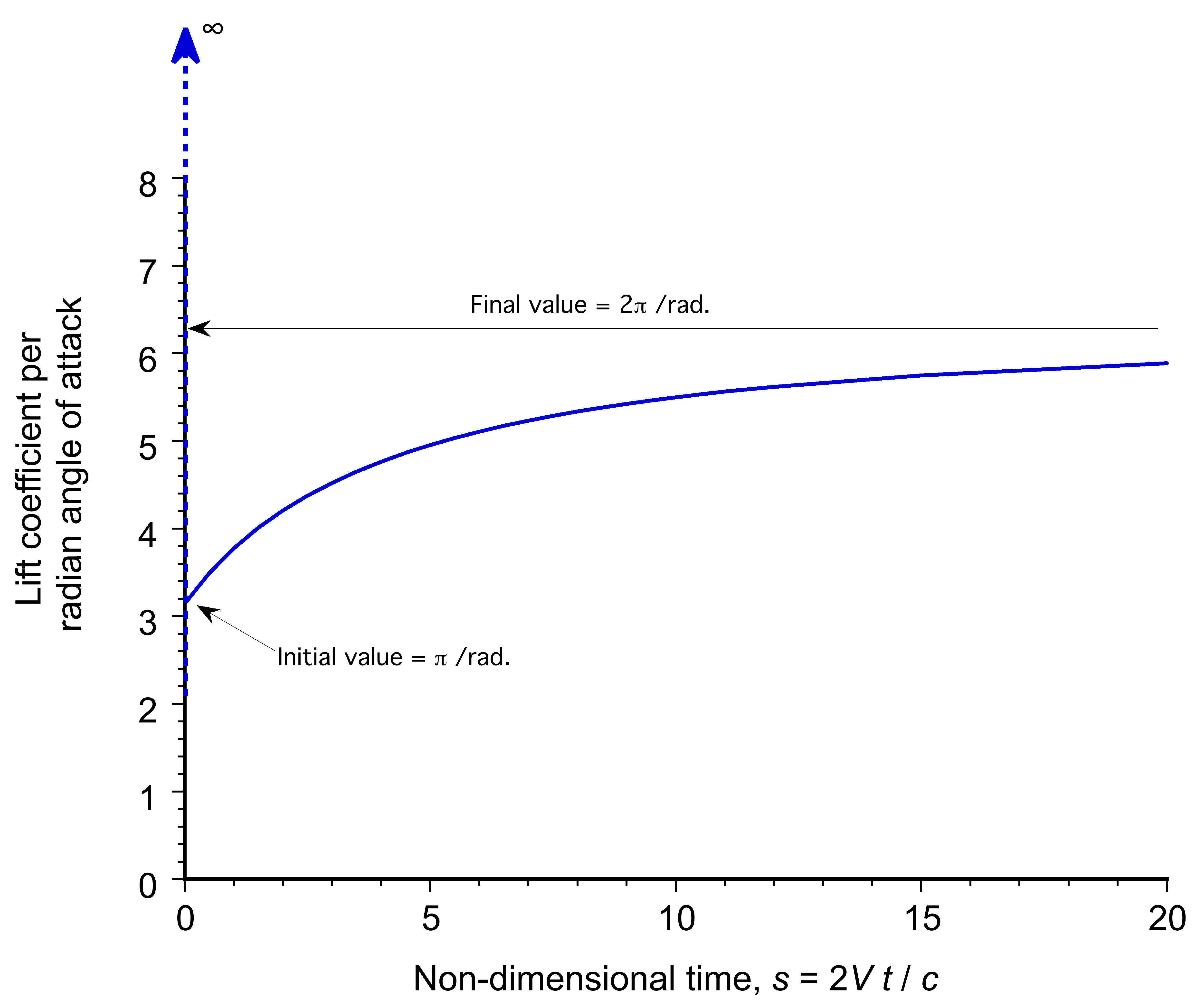
Wagner determined the transient lift response to a step change in $\alpha$ . This solution accounts for the effects of the shed wake using $\phi(s)$ . Wagner’s function $\phi(s)$ describes the circulatory effect of the shed wake. The lift coefficient is given by

(37) $\begin{equation*} C_l(t) = \frac{\pi c}{2V} \delta(t) + 2\pi \alpha \phi(s) \end{equation*}$

Because $\phi(s)$ builds asymptotically from $0.5$ to $1$ as $s \to \infty$ , then the lift builds from $\pi$ per radian angle of attack to $2\pi$ per radian, as shown in the figure below. There is an infinite spike at $s = 0$ because of the apparent mass term, and the function then starts at $\pi$ for $s = 0^+$ . Otherwise, the Wagner indicial response function represents the lift growth on the airfoil as the starting vortex is shed into the downstream wake and circulation builds around the airfoil.

The Wagner indicial response function is the lift response to a step change in the angle of attack.

For arbitrary variations in $\alpha(t)$ , the circulatory lift can be computed using the Duhamel integral, i.e.,

(38) $\begin{equation*} C_l^c(s) = 2\pi \left( \alpha(0)\phi(s) + \int_{0}^{s} \frac{d\alpha(\sigma)}{dt} \phi(s-\sigma) d\sigma \right) \end{equation*}$

Apparent mass terms are added to the circulatory component for the total lift. Numerical or approximate solutions are often used for practical calculations. Two-term exponential approximation (R.T. Jones, 1938, 1940), i.e.,

(39) $\begin{equation*} \phi(s) \approx 1.0 - 0.165 e^{-0.0455 s} - 0.335 e^{-0.3 s} \end{equation*}$

Approximations enable more straightforward computations while maintaining numerical accuracy.

Discretization of Duhamel Integral

Numerical integration must balance accuracy and computational efficiency. Assume two-term exponential form of $\phi(s)$ , i.e.,

(40) $\begin{equation*} \phi(s) = 1 - A_1 e^{-b_1 s} - A_2 e^{-b_2 s} \end{equation*}$

The effective angle of attack is given by

(41) $\begin{equation*} \alpha_e(s) = \alpha(s) - X(s) - Y(s) \end{equation*}$

where a recursive formula is used for $X(s)$ and $Y(s)$ , i.e.,

(42) $\begin{equation*} X(s+\Delta s) = X(s) e^{-b_1 \Delta s} + A_1 \Delta \alpha_s \quad \text{and} \quad Y(s+\Delta s) = Y(s) e^{-b_2 \Delta s} + A_2 \Delta \alpha_s \end{equation*}$

so that the effective angle of attack is given by

(43) $\begin{equation*} \alpha_e(s+\Delta s)) = \alpha(s+\Delta s)) - X(s+\Delta s)) - Y(s+\Delta s)) \end{equation*}$

The aerodynamic time history is contained in $X(s)$ and $Y(s)$ . The solution requires relatively small time steps for good accuracy, i.e., $b_1 \Delta s < 0.05$ .

Aeroelastic Analysis

The field of aeroelastics is not an easy one to master, but understanding the basics, and especially the underlying physics in a qualitative context, is the place to start. Flutter is a self-excited oscillation caused by the interaction of aerodynamic, elastic, and inertial forces. In a fairly general way, the structural dynamics of an aeroelastic system can be described by

(44) $\begin{equation*} M \,\overbigddot{q} + C \, \overbigdot{q} + K \, q = F_a \end{equation*}$

where $M$ is the mass matrix, $C$ is the damping matrix, $K$ is the stiffness matrix, $q$ is the displacement vector, and $F_a$ is the aerodynamic force vector. Aerodynamic forces can be computed using CFD, although panel methods or unsteady airfoil theory might also be used while appreciating their limitations. The aerodynamic force $F_a$ on the structure using CFD or panel methods is usually extracted from the pressure distribution, $p(x, y, z, t)$ , that acts over the surface, i.e.,

(45) $\begin{equation*} F_a (t) = \int_S p(t) \, d\vec{S} \end{equation*}$

where $\vec{S}$ is the unit normal vector area. Other methods, however, might be used to approximate aerodynamics, including unsteady airfoil theory m(Wagner function with the Duhamel integral), panel methods, etc. It is not unusual for flutter calculations to be made using various aerodynamic methods (and with different assumptions) and for the results to be compared.

Combining the aerodynamic and structural models then gives

(46) $\begin{equation*} M \, \overbigddot{q} + (C + B) \, \overbigdot{q} + (K + A) \, q = 0 \end{equation*}$

where $A$ and $B$ are called aerodynamic influence matrices. Flutter is a dynamic instability, and its condition is determined by solving

(47) $\begin{equation*} \underbrace{K + A - \omega^2 M}_{\rm Real~part} \ + \ i \, \underbrace{\omega (C + B)) \Phi}_{\rm Imaginary~part} = \Re (\omega) + i \, \Im (\omega) = 0 \end{equation*}$

where $\omega$ is the complex eigenvalue. Notice that $\Phi$ typically represents the mode shape or eigenvector associated with the eigenvalue. In the context of flutter analysis, $\Phi$ represents the deformation pattern of the structure at the flutter condition. Each eigenvalue has an associated eigenvector that describes how different points in the structure move relative to each other during an oscillation.

The “real” part, $\Re (\omega )$ , represents the balance between stiffness (including aerodynamic stiffness) and inertial forces, which is associated with the natural frequency of the system. When $\Re (\omega ) > 0$ , it indicates oscillatory motion. If $\Re (\omega ) = 0$ , it means a static aeroelastic response. For example, divergence is a static instability analyzed by setting dynamic terms to zero, i.e.,

(48) $\begin{equation*} (K + A) q = 0 \end{equation*}$

which means $q \rightarrow \infty$ , and the structure would theoretically deform infinitely under the aerodynamic loads. The critical divergence airspeed is found when the determinant of $(K + A) = 0$ . The “imaginary” part, $\Im (\omega )$ , represents the balance between damping (including aerodynamic damping) and the rate of change of displacement, which is associated with the damping of the system. If $\Im (\omega) > 0$ , it means positive damping (energy dissipation), while $\Im (\omega) < 0$ means negative damping (energy addition), which will extract energy from the flow and can lead to flutter.

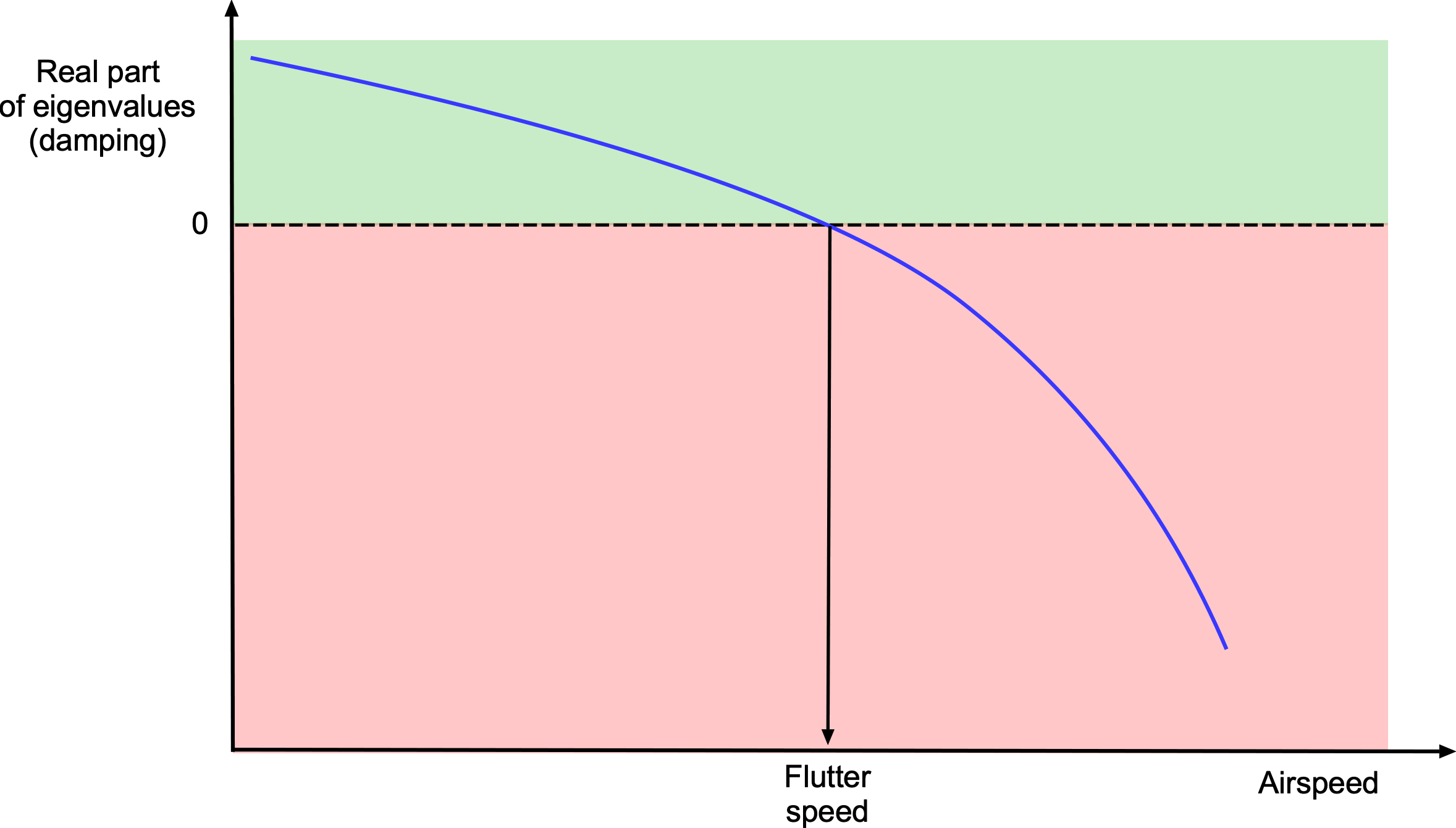
A typical flutter boundary is shown in the figure below, which plots the real part of the system eigenvalues, which is the damping, as a function of airspeed. The flutter speed is identified where the damping crosses zero, indicating the onset of an unstable oscillation. Notice that negative values indicate a stable system (damped motion), zero crossing marks the critical flutter speed, and positive values indicate instability (divergence from flutter).

A typical single degree-of-freedom flutter boundary in terms of the real part of the system eigenvalues (damping) as a function of airspeed.

The field of aeroelasticity also considers concepts such as limit cycle oscillations (LCO), where periodic self-sustained oscillations occur from nonlinearities in the aerodynamic or structural response. Engineers use sophisticated computational methods and experimental testing to predict and mitigate these aeroelastic phenomena, ensuring that aircraft and spacecraft designs meet stringent safety, performance, and certification standards in diverse flight conditions.

Torsional Flutter of a Cantilevered Wing

The understanding of the flutter mechanism is usually hidden in the relatively complex mathematics or inside some code that is being used as a “black box.” However, a classic exemplar to study for those being introduced to the field of aeroelasticity is a cantilever wing encastré at its root with a single degree of freedom in pitch (torsional motion), as shown in the figure below. Wings show smaller aerodynamic perturbations in bending and are also well-damped aerodynamically, so the torsional behavior is perhaps more instructive. The maximum airspeed of many aircraft is limited because of the onset of torsional flutter on the wings, which is a design compromise between wing strength, torsional rigidity, weight, and cost.

A cantilever wing encastré at its root with a single degree of freedom in pitch (torsional motion).

In this case, $q$ (the forcing) is equivalent to $\theta$ (the pitch angle), so the equation of motion is

(49) $\begin{equation*} I \, \overbigddot{\theta} + C \, \overbigdot{\theta} + K \, \theta = M_{\rm ac} \end{equation*}$

where $I$ is the mass moment of inertia per unit span about the elastic axis, $C$ is the structural damping coefficient (usually not much), $K$ is the torsional stiffness (mostly dictated by the wing box structure), and $M_{\rm ac}$ is the aerodynamic moment. Assuming quasi-steady aerodynamics,^[8] the aerodynamic moment per unit span can be written as

(50) $\begin{equation*} M_{\rm ac} = \frac{1}{2} \varrho \, V_{\infty}^2 \bar{c}^2 \, C_{m_\alpha} \theta \end{equation*}$

where $C_{m_\alpha}$ is the slope of the aerodynamic moment curve about the elastic axis and $\bar{c}$ is the mean wing chord. Notice that it can be assumed that any change in aerodynamic angle of attack, $\alpha$ , is proportional to the change in $\theta$ . Therefore, the equation of motion becomes

(51) $\begin{equation*} I \, \overbigddot{\theta} + C \, \overbigdot{\theta} + K \, \theta = \frac{1}{2} \varrho \, V_{\infty}^2 c^2 \, C_{m_\alpha} \theta \end{equation*}$

which is the equation to be solved for $\theta(t)$ .

Analytical Approach to Flutter

A direct approach to finding the flutter speed can be used. Assume a trial solution to the equation of motion of the oscillatory form

(52) $\begin{equation*} \theta(t) = \theta_0 \, e^{i \omega t} \end{equation*}$

Differentiating once and twice gives

(53) $\begin{equation*} \overbigddot{\theta}(t) = -\omega^2 \, \theta_0 \, e^{i \omega t} \quad \mbox{and} \quad \overbigdot{\theta}(t) = i \, \omega \, \theta_0 \, e^{i \omega t} \end{equation*}$

Substituting these results into the equation of motion gives

(54) $\begin{equation*} I (-\omega^2 \, \theta_0 \, e^{i \omega t}) + C (i \omega \, \theta_0 \, e^{i \omega t}) + K (\theta_0 \, e^{i \omega t}) = \frac{1}{2} \varrho \, V_{\infty}^2 \, c^2 \, C_{m_\alpha} (\theta_0 \, e^{i \omega t}) \end{equation*}$

where $K$ is the torsional stiffness, i.e., $K = G \, J$ , where $G$ is the shear modulus and $J$ is the second moment of area of the section. Simplifying gives

(55) $\begin{equation*} -I \, \omega^2 + i \, C \omega + K = \frac{1}{2} \varrho \, V_{\infty}^2 \, c^2 \, C_{m_\alpha} \end{equation*}$

This latter equation can now be rearranged to form the characteristic equation, i.e.,

(56) $\begin{equation*} -I \, \omega^2 + i \, C \omega + K - \frac{1}{2} \varrho \, V_{\infty}^2 \, c^2 \, C_{m_\alpha} = 0 \end{equation*}$

The real and imaginary parts of the equation can be separated to determine if flutter will occur. For the real part, then

(57) $\begin{equation*} \Re = -I \omega^2 + K = \frac{1}{2} \varrho \, V_{\infty}^2 \, c^2 \, C_{m_\alpha} \end{equation*}$

and for the imaginary part, then

(58) $\begin{equation*} \Im = i \, C \, \omega = 0 \end{equation*}$

If it is assumed that there is no structural damping, i.e., $C = 0$ , then

(59) $\begin{equation*} -I \, \omega^2 + K = \frac{1}{2} \varrho \, V_f^2 \, \bar{c}^2 \, C_{m_\alpha} \end{equation*}$

where $V_f$ is the critical airspeed at which flutter will occur. Setting $\omega = 0$ allows the airspeed at which the system becomes unstable to be found, i.e.,

(60) $\begin{equation*} K = \frac{1}{2} \varrho \, V_f^2 \, \bar{c}^2 C_{m_\alpha} \end{equation*}$

Rearranging gives the critical flutter speed as

(61) $\begin{equation*} V_f = \sqrt{\frac{2 K}{\varrho \, \bar{c}^2 \, C_{m_\alpha}}} \end{equation*}$

This exemplar illustrates how aerodynamic forces interact with the structural dynamics of the wing, influencing its aeroelastic stability. Aeroelastic analysis of such systems is crucial for designing aircraft wings that can withstand aerodynamic loads while maintaining stability and structural integrity. Notice from Eq. 61 that, in this case, the flutter speed is proportional to the square root of the ratio of the torsional stiffness to the aerodynamic effects. Making the wing stiffer will increase the flutter speed, but the downside is that it will also increase structural weight and cost.

Time-Marching Solution

There are different ways to find the solution to the torsional flutter problem. One approach is a numerical integration method, which can integrate the equations of motion by marching in time. First, a time step $\Delta t$ must be chosen that is small enough to capture the response accurately. Second, set initial values for $\theta(0)$ and $\overbigdot{\theta}(0)$ , which represent a disturbance to excite the aeroelastic system. Physically, such a disturbance could be a gust or a sudden flight control input. During flight testing, mechanical shakers excite the structure at different frequencies to examine possible aeroelastic problems or flutter.

Then, a numerical integration method, such as the Euler method (which is only first-order accurate) or a Runge-Kutta method (much more accurate but more computationally expensive), can be used to update the solution at each step, i.e.,

(62) $\begin{equation*} \overbigdot{\theta}_{n+1} = \overbigdot{\theta}_n + \overbigddot{\theta}_n \, \Delta t \quad \mbox{and} \quad \theta_{n+1} = \theta_n + \overbigdot{\theta}_n \, \Delta t \end{equation*}$

The values of $\overbigddot{\theta}_n$ can be computed based on the current values of $\theta_n$ and $\overbigdot{\theta}_n$ . The aerodynamic moment on the wing, $M_a$ , at each time step can be computed based on the current values of $\theta_n$ and $V_n$ ; usually $V_n$ = $V_{\infty}$ = constant. Unsteady effects can be incorporated using the indicial method with superposition in the form of the numerical solution to the Duhamel integral, as previously described. Then, the process continues by marching the aerodynamic and the structural response until the desired end time or a specified condition, such as flutter onset.

The figure below shows typical results that can be obtained from the time-marching process. Suppose nothing happens after a long time period. In that case, the process can be repeated for other airspeeds or for variations in the different parameters, such as the center of gravity location, which affects the torsional inertia about the elastic axis (ea). Depending on the wing design, its aeroelastic response can be well-damped, showing a limit cycle oscillation, a classic form of diverging flutter, or rapid divergence. The process would be repeated for different airspeeds and values of air density (density altitude) to estimate the stability boundaries for the structure or the entire aircraft.

The frequency and damping of two structural modes as a function of airspeed show that the likelihood of flutter increases if the structural frequencies begin to coalesce.

Flutter of a Two-Dimensional Airfoil Section

The flutter of a two-dimensional (2D) airfoil section is a more tangible case to study. Consider a two-degree-of-freedom model for a typical 2D airfoil section that can undergo: 1. Plunge motion $h(t)$ , which represents vertical displacement (typically at 1/4-chord for thin airfoils in subsonic flow), 2. Pitch motion $\theta(t)$ , which represents rotation about the elastic axis (pivot point of torsional motion).

Two-dimensional section used for flutter analysis.

The parameter $a$ represents the non-dimensional location of the elastic axis relative to the aerodynamic center. The elastic axis (ea) is located at a non-dimensionalized distance $a$ from the aerodynamic center (ac), i.e.,

(63) $\begin{equation*} a = \frac{x_{\text{ea}} - x_{\text{ac}}}{b} \end{equation*}$

If $a = 0$ , the elastic axis coincides with the aerodynamic center (usually at the 1/4-chord). If $a > 0$ , the elastic axis is located aft of the aerodynamic center. If $a < 0$ , the elastic axis is located forward of the aerodynamic center. The value of $a$ affects the aerodynamic moment arm and thus influences the coupling between plunge ( $h$ ) and pitch ( $\theta$ ) motions in a flutter analysis.

The governing equations for the plunge and pitch degrees of freedom are given by

(64) $\begin{equation*} m \overbigddot{h} + S_{\alpha} \overbigddot{\theta} + K_h h = L' \quad \text{and} \quad S_{\alpha} \overbigddot{h} + I_{\alpha} \overbigddot{\theta} + K_{\alpha} \theta = M' \end{equation*}$

where:

$m$ = mass per unit span.
$S_{\alpha} = m x_{\alpha} b$ (static moment about the elastic axis).
$I_{\alpha} = m r_{\alpha}^2 \, b^2$ (mass moment of inertia about the elastic axis, where $r_{\alpha}$ is the radius of gyration).
$K_h$ = bending stiffness (plunge stiffness).
$K_{\alpha}$ = torsional stiffness (pitch stiffness).
$L'$ = aerodynamic lift force per unit span.
$M'$ = aerodynamic pitching moment per unit span.

The aerodynamic forces (lift $L'$ and moment $M'$ ) are derived from thin airfoil theory using quasi-steady aerodynamics, i.e.,

(65) $\begin{equation*} L' = \frac{1}{2} \varrho V_{\infty}^2 (2b) C_l \quad \text{and} \quad M' = \frac{1}{2} \varrho V_{\infty}^2 (2b)^2 C_m \end{equation*}$

where the lift coefficient $C_l$ and moment coefficient $C_m$ are given by

(66) $\begin{equation*} C_l = 2\pi \left( \frac{h}{b} + \left(a + \frac{1}{2}\right) \theta + \frac{\overbigdot{h}}{V} + \left(a + \frac{1}{2} \right) \frac{b\overbigdot{\theta}}{V} \right) \end{equation*}$

and

(67) $\begin{equation*} C_m = -\pi \left( \left(\frac{1}{2} + a\right) \frac{h}{b} + \left( \frac{1}{8} + a^2 \right) \theta + \left( \frac{1}{2} + a \right) \frac{\overbigdot{h}}{V} + \left( \frac{1}{8} + a^2 \right) \frac{b\overbigdot{\theta}}{V} \right) \end{equation*}$

Therefore, the lift and pitching moment are given by

(68) $\begin{equation*} L' = \frac{1}{2} \varrho V_{\infty}^2 (2b) \, 2\pi \left( \frac{h}{b} + \left(a + \frac{1}{2}\right) \theta + \frac{\overbigdot{h}}{V} + \left(a + \frac{1}{2} \right) \frac{b\overbigdot{\theta}}{V} \right) \end{equation*}$

and

(69) $\begin{equation*} M' = \frac{1}{2} \varrho V_{\infty}^2 (2b)^2 \, (-\pi) \left( \left(\frac{1}{2} + a\right) \frac{h}{b} + \left( \frac{1}{8} + a^2 \right) \theta + \left( \frac{1}{2} + a \right) \frac{\overbigdot{h}}{V} + \left( \frac{1}{8} + a^2 \right) \frac{b\overbigdot{\theta}}{V} \right) \end{equation*}$

Substituting $L'$ and $M'$ into the equations of motion gives

(70) $\begin{equation*} \begin{bmatrix} m & S_{\alpha} \\[6pt] S_{\alpha} & I_{\alpha} \end{bmatrix} \begin{bmatrix} \overbigddot{h} \\[6pt] \overbigddot{\theta} \end{bmatrix} + \begin{bmatrix} K_h & 0 \\[6pt] 0 & K_{\alpha} \end{bmatrix} \begin{bmatrix} h \\[6pt] \theta \end{bmatrix} = \frac{1}{2} \varrho V_{\infty}^2 (2b) \begin{bmatrix} 2\pi & 2\pi \left( a + \dfrac{1}{2} \right) \\[10pt] -\pi \left( \dfrac{1}{2} + a \right) & -\pi \left( \dfrac{1}{8} + a^2 \right) \end{bmatrix} \begin{bmatrix} h \\[18pt] \theta \end{bmatrix} \end{equation*}$

For flutter, a non-trivial solution requires that the determinant of the coefficient matrix must be zero, i.e.,

(71) $\begin{equation*} \begin{vmatrix} m - \frac{1}{2} \varrho V_{\infty}^2 A b^{-1} & S_{\alpha} - \dfrac{1}{2} \varrho V_{\infty}^2 A \left(a + \dfrac{1}{2}\right) \\[12pt] S_{\alpha} + \dfrac{1}{2} \varrho V_{\infty}^2 B \left(\dfrac{1}{2} + a\right) & I_{\alpha} + K_{\alpha} - \dfrac{1}{2} \varrho V_{\infty}^2 B \left(\dfrac{1}{8} + a^2\right) \end{vmatrix} = 0 \end{equation*}$

where $A = 2 \pi b$ and $B = \pi b^2$ . Solving for $V_f$ gives

(72) $\begin{equation*} V_f = \sqrt{\dfrac{(K_h I_{\alpha} - S_{\alpha}^2)}{\dfrac{1}{2} \varrho b^2 (m r_\alpha^2 + m x_\alpha^2)}} \end{equation*}$

Worked Example #3

Consider a uniform, symmetric wing section with the following properties:

Semi-chord: $b$ = 0.5 m.
Mass per unit span: $m$ = 10 kg/m.
Aerodynamic center to elastic axis distance: $a$ = -0.3 (normalized by $b$ ).
Center of mass to elastic axis distance: $x_\alpha$ = -0.2 $b$ .
Radius of gyration about the elastic axis: $r_\alpha$ = 0.5 $b$ .
Bending stiffness: $k_h$ = 10,000 N/m.
Torsional stiffness: $k_\alpha$ = 500 Nm/rad.
Air density: $\varrho$ = 1.225 kg/m $^3$ .

Determine the flutter speed. Assume quasi-steady aerodynamics.

Show solution/hide solution.

The flutter speed can be estimated using the classical two-degree-of-freedom model, i.e.,

$m \overbigddot{h} + S_{\alpha} \overbigddot{\theta} + k_h h = L, \quad \text{and} \quad S_{\alpha} \overbigddot{h} + I_{\alpha} \overbigddot{\theta} + K_{\alpha} \theta = M$

where $S_{\alpha} = m x_\alpha b$ is the static moment of the system, $I_{\alpha} = m r_\alpha^2 b^2$ is the mass moment of inertia}, and $L$ and $M$ are the aerodynamic lift and moment, respectively.

For an approximate flutter speed calculation, then the empirical flutter determinant equation can be used, i.e.,

$V_f = \sqrt{\frac{(k_h I_{\alpha} - S_{\alpha}^2)}{\frac{1}{2} \varrho b^2 (m r_\alpha^2 + m x_\alpha^2)}}$

The static moment is

$S_{\alpha} = m x_{\alpha} b = 10 (-0.2 \times 0.5) = -1.0 \text{ kg m}$

The mass moment of inertia is

$I_{\alpha} = m r_{\alpha}^2 b^2 = 10 (0.5)^2 (0.5)^2 = 1.25 \text{ kg m²}$

Therefore, the flutter speed is

$V_f = \sqrt{\frac{(10000 \times 1.25 - (-1)^2)}{\frac{1}{2} \times 1.225 \times (0.5)^2 \times (10 \times 0.25 + 10 \times 0.04)}}$

and simplifying gives

$V_f = \sqrt{\frac{(12500 - 1)}{0.6125 \times (2.9)}} = \sqrt{\frac{12499}{1.776}} = 83.9 \text{ m/s}$

The estimated flutter speed for the given wing is 83.9 m/s. If the aircraft is expected to operate near or beyond this speed, modifications such as increasing stiffness or mass distribution adjustments are necessary to prevent flutter.

Why use quasi-steady aerodynamics in initial flutter analysis?

Quasi-steady aerodynamics is used in initial flutter analysis because it provides a simple closed-form flutter speed equation, making it easier to obtain quick analytical insights. It is particularly effective for low-frequency, low-speed applications where unsteady aerodynamic effects are minimal. Additionally, it serves as a valid first approximation before employing more advanced unsteady aerodynamic models and computational methods such as Theodorsen’s theory for 2D airfoils or numerical approaches like the doublet lattice method and CFD.

Flutter Speed Determination Using Theodorsen’s Function

To more accurately predict the flutter speed of a 2D airfoil section, it is necessary to include unsteady aerodynamic effects, which are captured using Theodorsen’s function. However, in this case, an interactive method must be used. The aerodynamic lift and moment in unsteady flow are modified using Theodorsen’s function $C(k)$ , i.e.,

(73) $\begin{equation*} L' = \frac{1}{2} \varrho V_{\infty}^2 (2b) \, 2\pi C(k) \left( \frac{h}{b} + \left(a + \frac{1}{2}\right) \theta + \frac{\overbigdot{h}}{V} + \left(a + \frac{1}{2} \right) \frac{b\overbigdot{\theta}}{V_{\infty}} \right) \end{equation*}$

and

(74) $\begin{equation*} M' = \frac{1}{2} \varrho V_{\infty}^2 (2b)^2 \, C(k) \, \left(-\pi \left( \left(\frac{1}{2} + a\right) \frac{h}{b} + \left( \frac{1}{8} + a^2 \right) \theta + \left( \frac{1}{2} + a \right) \frac{\overbigdot{h}}{V_{\infty}} + \left( \frac{1}{8} + a^2 \right) \frac{b\overbigdot{\theta}}{V_{\infty}} \right) \right) \end{equation*}$

Substituting the expressions for $L'$ and $M'$ into the structural equations of motion results in:

(75) $\begin{equation*} m \overbigddot{h} + S_{\alpha} \overbigddot{\theta} + k_h h = \frac{1}{2} \varrho V_{\infty}^2 b 2\pi C(k) \left( \frac{h}{b} + \left(a + \frac{1}{2}\right) \theta + \frac{\overbigdot{h}}{V_{\infty}} + \left(a + \frac{1}{2} \right) \frac{b\overbigdot{\theta}}{V_{\infty}} \right) \end{equation*}$

and

(76) $\begin{equation*} S_{\alpha} \overbigddot{h} + I_{\alpha} \overbigddot{\theta} + K_{\alpha} \theta = -\frac{1}{2} \varrho V_{\infty}^2 b^2 \pi C(k) \left( \left(\frac{1}{2} + a\right) \frac{h}{b} + \left( \frac{1}{8} + a^2 \right) \theta + \left( \frac{1}{2} + a \right) \frac{\overbigdot{h}}{V_{\infty}} + \left( \frac{1}{8} + a^2 \right) \frac{b\overbigdot{\theta}}{V} \right) \end{equation*}$

Rewriting in matrix form gives

(77) $\begin{equation*} \begin{bmatrix} m & S_{\alpha} \\[8pt] S_{\alpha} & I_{\alpha} \end{bmatrix} \begin{bmatrix} \overbigddot{h} \\[8pt] \overbigddot{\theta} \end{bmatrix} + \begin{bmatrix} k_h & 0 \\[8pt] 0 & k_{\alpha} \end{bmatrix} \begin{bmatrix} h \\[8pt] \theta \end{bmatrix} = \text{\small Unsteady aerodynamics} \end{equation*}$

Expanding with Theodorsen’s function, the determinant condition for flutter is

(78) $\begin{equation*} \begin{vmatrix} m - \dfrac{1}{2} \varrho V_{\infty}^2 \, A \, C(k) b^{-1} & S_{\alpha} - \dfrac{1}{2} \varrho V_{\infty}^2 A \, C(k) \left(a + \dfrac{1}{2}\right) \\[14pt] S_{\alpha} + \dfrac{1}{2} \varrho V_{\infty}^2 \, B \, C(k) \left(\dfrac{1}{2} + a\right) & I_{\alpha} + K_{\alpha} - \dfrac{1}{2} \varrho V_{\infty}^2 \, B \, C(k) \left(\dfrac{1}{8} + a^2\right) \end{vmatrix} = 0 \end{equation*}$

Notice that the quasi-steady case is recovered if $C(k)=1$ , i.e., $k$ = 0.

The flutter speed can be estimated by solving this determinant equation iteratively. Because $C(k)$ depends on the reduced frequency $k$ , an iterative approach is necessary. The steps are:

Assume an initial flutter frequency, i.e., $\omega_f$ .
Compute the reduced frequency at the flutter speed, $k_f = \dfrac{\omega_f c}{2 V_f} = \dfrac{\omega_f b}{V_f}$ .
Evaluate Theodorsen’s function at the flutter speed, $C(k_f)$ .
Solve for the new flutter speed, $V_f$ .
Iterate steps 1 through 4 until convergence is obtained on $V_f$ .

For an approximate analytical solution, the flutter speed can be estimated using quasi-steady aerodynamics, i.e.,

(79) $\begin{equation*} V_f \approx \sqrt{\dfrac{(k_h I_{\alpha} - S_{\alpha}^2)}{\dfrac{1}{2} \varrho b^2 (m r_\alpha^2 + m x_\alpha^2) \, C(k_f)}} \end{equation*}$

Flutter Using FEM/CFD Coupling

The aeroelastic process must be conducted either by time-marching or by an iterative process. An iterative coupling process will typically proceed along these lines:

Define the geometry and grids for FEM and CFD. They will differ because the grids required to solve the aerodynamics have different requirements than the structural shape.
$\[\]$
Apply the material properties and boundary conditions in the FEM. Using isotropic material such as aluminum will have different properties to composites.
$\[\]$
Set up the CFD with the defined flow conditions or use any other selected aerodynamic model, e.g., a panel method.
$\[\]$
Compute the aerodynamic forces, $F_a$ , from the selected aerodynamic model.
Update the FEM model with aerodynamic forces $F_a$ .
Iterate between CFD and FEM to capture aeroelastic interactions, i.e., couple the aerodynamics and structural dynamics in the form
$\[\]$

(80) $\begin{equation*} M \, \overbigddot{q} + (C + B) \, \overbigdot{q} + (K + A) \, q = 0 \end{equation*}$

$\[\]$
Repeat the FEM analysis for the resulting structural response on the deformed structure.
$\[\]$
Conducted CFD simulations of the deformed structure to obtain new aerodynamic loads.
$\[\]$
Exchange data between FEM and CFD to formalize the coupled analysis.
$\[\]$
Analyze displacements, stresses, and aerodynamic forces.
$\[\]$
Evaluate the results against the stability criteria for flutter or divergence.

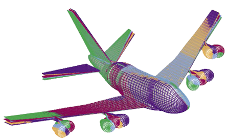
By integrating CFD and FEM, engineers can accurately predict and analyze aeroelastic phenomena, ensuring the safety and performance of aerospace structures. For example, this process has been applied to large aircraft such as the Boeing 747, as shown in the figure below. These results provide valuable information on the stiffness of airframe components, helping to prevent aeroelastic and flutter issues before the first flight. However, flight testing is essential to validate these calculations and ensure the aircraft is flutter-free across its operational flight envelope.

A model created by ZONA Technology shows aircraft deformations due to flutter. — A finite-element flutter model of a Boeing 747 created by ZONA Technology shows aircraft deformations resulting from flutter.

Flutter Occurences in Practice

In practice, aircraft structures can exhibit coupled responses between different “modes,” e.g., between wing torsion and bending, between the engine mount and the wing, or between the wing and a control surface. Two fatal crashes of the Lockheed Electra were attributed to a phenomenon called “pylon whirl flutter,” where the aerodynamic excitations from the propeller coupled with the natural frequency of the wing, which entered into a destructive resonant vibration and catastrophic flutter. Extensive structural modifications were made to the Electra’s design, including changes to the wings and the engine mounts to increase their stiffness.

During its first flight tests, the Boeing Dash 80 (predecessor to the Boeing 707) experienced aileron flutter, after which modifications were made to the control system. This incident underscored the importance of flutter testing for jet airliners and led to improvements in the control surface design and testing protocols. The Boeing 747 encountered unexpected flutter on its horizontal stabilizers during its flight test program, and the Boeing 747-8 suffered from wing tip flutter issues before resolution.^[9]

The interaction between all structural modes must be represented on an aircraft to account for the overall coupled dynamic behavior of the structure. Inevitably, this requires a comprehensive CFD and structural dynamic analysis. The process involves solving the coupled equations describing the entire structure and the aerodynamics, and finding the eigenvalues that represent the system’s natural frequencies and damping ratios, as outlined previously. The figure below shows an example of the information that can be extracted from this type of aeroelastic analysis, which shows the frequency and damping as a function of airspeed or dynamic pressure should be used more appropriately.

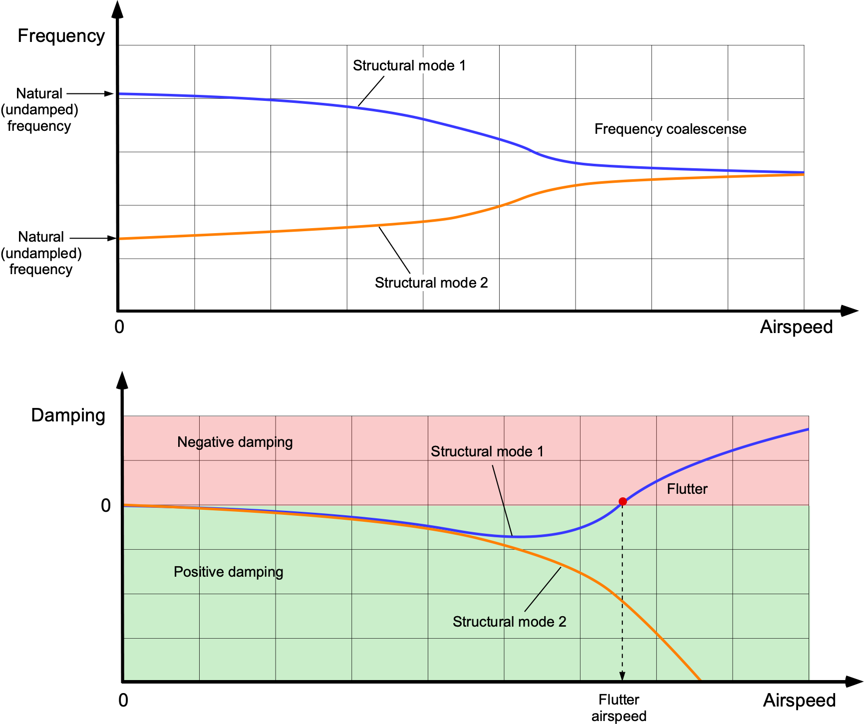
The frequency and damping of two structural modes as a function of airspeed, showing that flutter is likely to occur near frequency coalescence. — The frequency and damping of two structural modes as a function of airspeed showing that flutter is likely to occur near frequency coalescence.

The frequency and damping of two structural modes as a function of airspeed show that the likelihood of flutter increases if the structural frequencies begin to coalesce. The undamped zero airspeed frequencies are distinct at low speeds, and the system remains stable. As the airspeed increases, the aerodynamic forces acting on the structure also increase. These forces change the frequencies of the structure because they add an effective aerodynamic stiffness and damping to the system, which in some cases may cause the frequencies to change so that they start converging, a phenomenon known as frequency coalescence. This condition results in a continuous energy exchange between the aerodynamic forces and the elastic energy stored in structural vibrations and overcomes structural damping.

Flutter will likely arise if the net structural-aerodynamic damping of the aeroelastic system becomes negative. In this condition, aerodynamic forces feed energy into the structural mode at a rate that exceeds the damping at a frequency that matches the structure’s natural frequency. If the energy input from the aerodynamics exceeds the structure’s inherent damping forces, the oscillations grow exponentially, leading to flutter.

Flight Control Reversal

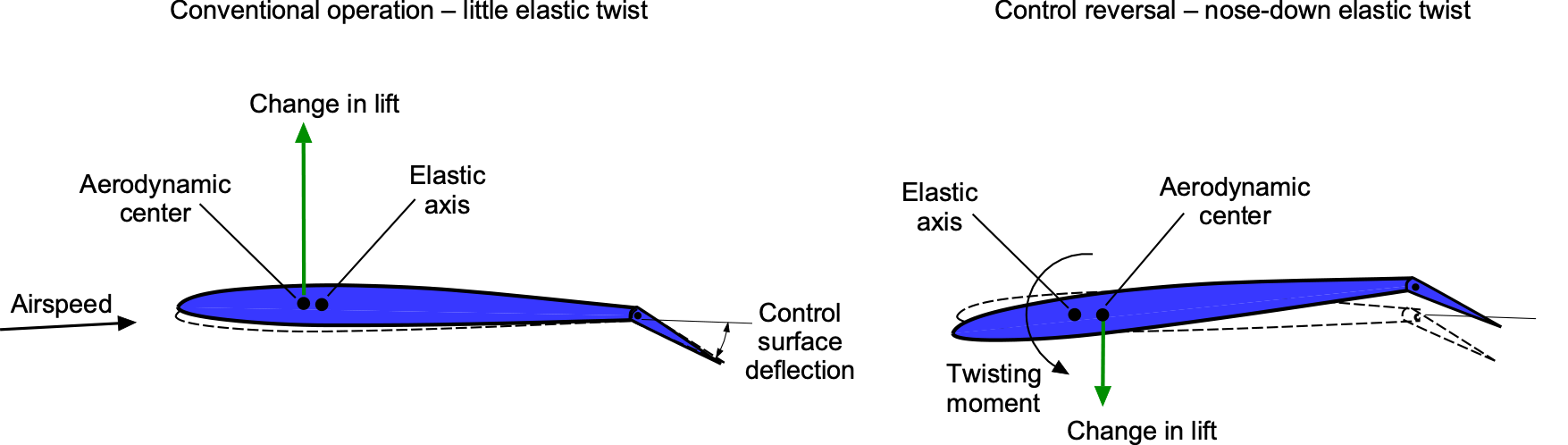
Control reversal occurs when a control surface deflection, such as an aileron, rudder, or elevator, responds opposite to the pilot’s intended input because of aerodynamic and structural interactions. This behavior typically occurs at higher airspeeds when the aerodynamic forces acting on the control surface may induce excessive structural deformations, particularly in the wing or tail section. Suppose a pilot applies aileron inputs to roll the aircraft, for example, the aerodynamic forces on the wing may cause it to twist so that the effective angle of attack increases instead of decreases, leading to an unintended rolling motion in the opposite direction, as shown in the figure below.

A wing section without sufficient torsional stiffness can exhibit control reversal where the opposite effect is obtained from control inputs.

This undesirable effect is particularly pronounced in aircraft with long, slender wings, such as sailplanes, or any type of wings with insufficient torsional stiffness. In an attempt to minimize structural weight, sometimes wing skins are too thin to give the needed torsional stiffness. Historically, roll or aileron reversal was a significant issue in high-performance fighter airplanes during WW2, as well as early jet airplanes. Some aircraft, such as the Supermarine Spitfire, experienced aileron reversal at high speeds, limiting their maneuverability in combat. Another contributing factor is the shifting of the aerodynamic center with increasing speed. If the aircraft is not adequately designed to counteract these forces, control effectiveness can degrade as speed increases, eventually leading to reversal. This issue was common in early high-speed aircraft before engineers developed techniques to counteract it.

To mitigate control reversal, engineers may employ several strategies. Increasing the stiffness of the aircraft’s structure, particularly in the wing and empennage, is usually very effective in resisting excessive structural twisting or bending. Mass balancing, where weights are strategically placed to adjust the center of gravity of control surfaces, can also reduce the tendency for control reversal, the extra weight giving a favorable gravity and inertial moment. On modern high-speed aircraft, powered control systems, such as hydraulic or fly-by-wire actuators, can mitigate any aeroelastic problems by ensuring that pilot inputs will always be applied to minimize structural flexing.

Dynamic Stall & Stall Flutter

Stall flutter is another aeroelastic phenomenon that occurs when flow separation leads to unsteady aerodynamic forces and potentially oscillatory structural instability. It is relevant in various aerospace and engineering applications, where predicting and mitigating its effects are essential for ensuring structural integrity and aerodynamic performance. Understanding stall flutter requires nonlinear aerodynamic modeling and experimental validation to develop practical mitigation steps and design improvements.

Dynamic Stall

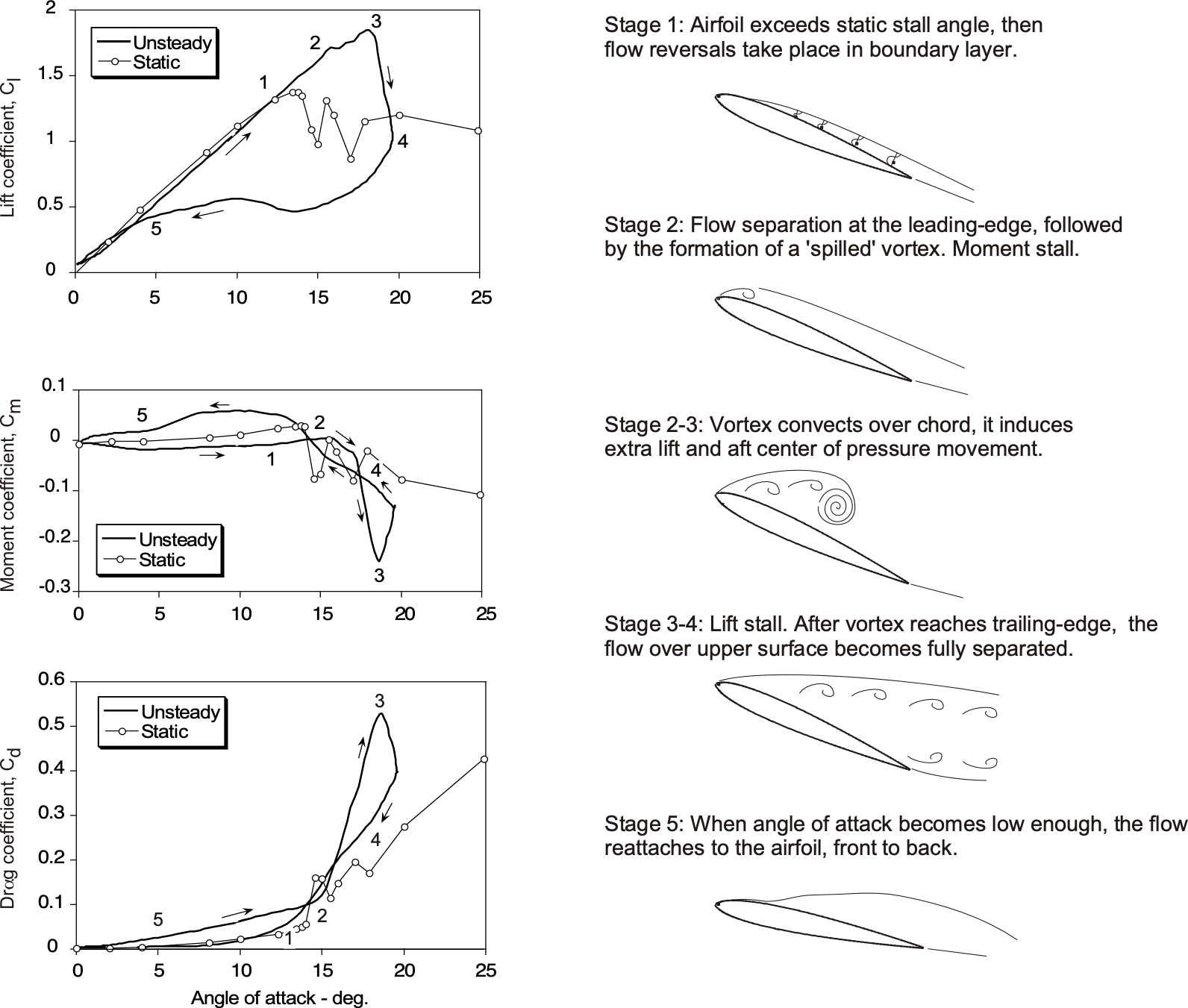
Under unsteady conditions, airfoils and wings behave differently than in steady flow. In particular, their stall characteristics are very different, and this behavior is called a dynamic stall. This phenomenon has received much research interest because of its unsteady aerodynamic effects, including the shedding of a leading-edge vortex, as shown in the simulation below. The onset of a dynamic stall can lead to another type of aeroelastic behavior called stall flutter, which can occur on helicopter blades.

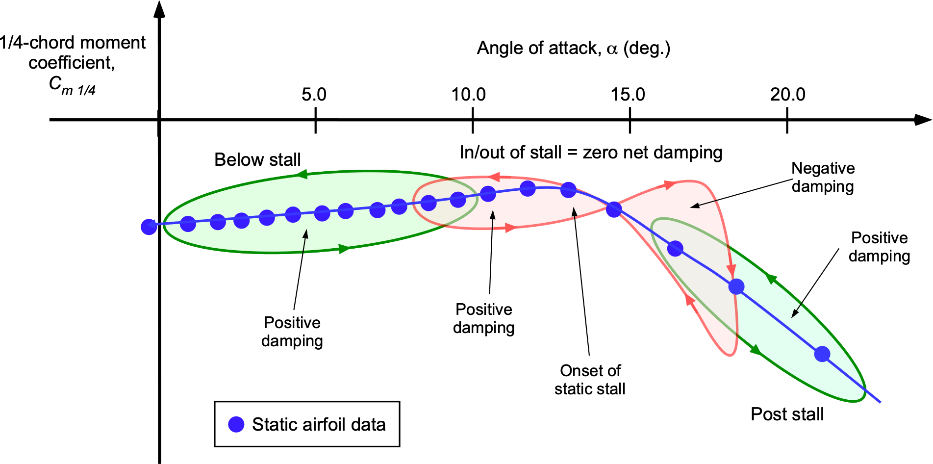
Vortex shedding increases lift and drag, giving powerful nose-down (negative) pitching moments because of the aft-moving center of pressure induced by the shedding vortex, as shown in the figure below, based on measurements and flow visualization. Dynamic stall is known for exhibiting higher levels of maximum lift, drag, and pitching moments and hysteresis effects that can lead to flutter phenomena. It is particularly relevant in designing and analyzing helicopter rotors, wind turbine blades, and specific aircraft configurations.

Dynamic stall characteristics are very different from what happens under steady conditions.

Engineers and researchers study the phenomenon of dynamic stall to understand the effects better and develop strategies to mitigate any adverse impact on the performance of aerospace systems. In particular, helicopter rotor blades often experience dynamic stall during higher-speed forward flight or during maneuvers. Indeed, the onset of dynamic stall limits the helicopter’s operational flight envelope. Wind turbine blades may encounter dynamic stall during sudden changes in wind conditions, leading to variations in power output and high blade loads that may produce concerning vibration levels. Aircraft wings can also undergo dynamic stall during aggressive maneuvers, which is a behavior that must be considered when establishing the maneuvering flight envelope for military combat aircraft.

Stall Flutter

Stall flutter is a nonlinear aeroelastic phenomenon that occurs when an airfoil or structure experiences flow separation. This separation leads to unsteady aerodynamic forces and oscillatory instabilities. Unlike classical flutter, which occurs in a linear aerodynamic regime before stall, stall flutter happens post-stall, when the flow has already separated from the surface. Because of its dependence on unsteady, nonlinear aerodynamics, stall flutter is more complex to analyze and predict.

The primary cause of stall flutter is flow separation, which occurs when the angle of attack exceeds the critical stall limit. Dynamic stall further intensifies this phenomenon, as the lags in periodic flow separation and reattachment generate reduced or even negative aerodynamic damping, as shown in the figure below in terms of pitching moment. Additionally, limited structural damping in a structure to dissipate the unsteady energy can lead to stall flutter.

Reduced aerodynamic damping at or near stall can lead to stall flutter.

Stall flutter can be an issue for wings and control surfaces, such as flaps and ailerons, at high angles of attack. Helicopter rotor blades have been known to encounter stall flutter in the retreating blade region, where local angles of attack can become high during forward flight. Stall flutter can also affect compressor and turbine blades in jet engines, where unsteady flow interactions are crucial in their performance. Civil engineering structures like bridges and tall buildings may experience vortex-induced oscillations resembling stall flutter behavior.

Mathematically, stall flutter is challenging to model because of its nonlinear nature. Traditional linear aeroelastic models, such as Theodorsen’s theory on the linear indicial response method, are insufficient because they assume attached flow. Instead, nonlinear aerodynamic models are required to capture the complex flow physics. Semi-empirical models, like the Leishman-Beddoes dynamic stall model, provide approximations for the unsteady aerodynamic forces that could be potentially encountered in stall flutter. Coupled fluid-structure interaction simulations are used to study the effects of separated flow on structural vibrations. Mitigating stall flutter involves several approaches, such as modifying the airfoil’s geometry, helping delay flow separation, and reducing vortex shedding effects. Increasing structural stiffness and damping can also help dissipate energy and suppress structural response.

Buffeting & Buzzing

While buffeting, buzzing, and stall flutter are all aeroelastic problems involving unsteady aerodynamic forces, they differ in their fundamental mechanisms. Buffeting is a forced, low-frequency vibration caused by turbulence or separated flow impingement on a surface. Buzzing is a self-excited, high-frequency oscillation of control surfaces, often because of aeroelastic feedback and insufficient damping.

Buffeting

Buffeting is a random, low-frequency, forced vibration caused by unsteady aerodynamic forces acting on a structure. It typically occurs when a lifting surface, such as an aircraft wing or tailplane, is subjected to turbulence or wake disturbances from another part of the airplane. One of the most common causes of buffeting is flow separation and vortex shedding behind a stalled airfoil. When a surface encounters separated flow, turbulent eddies form and impinge on downstream airframe structures, generating fluctuating forces.

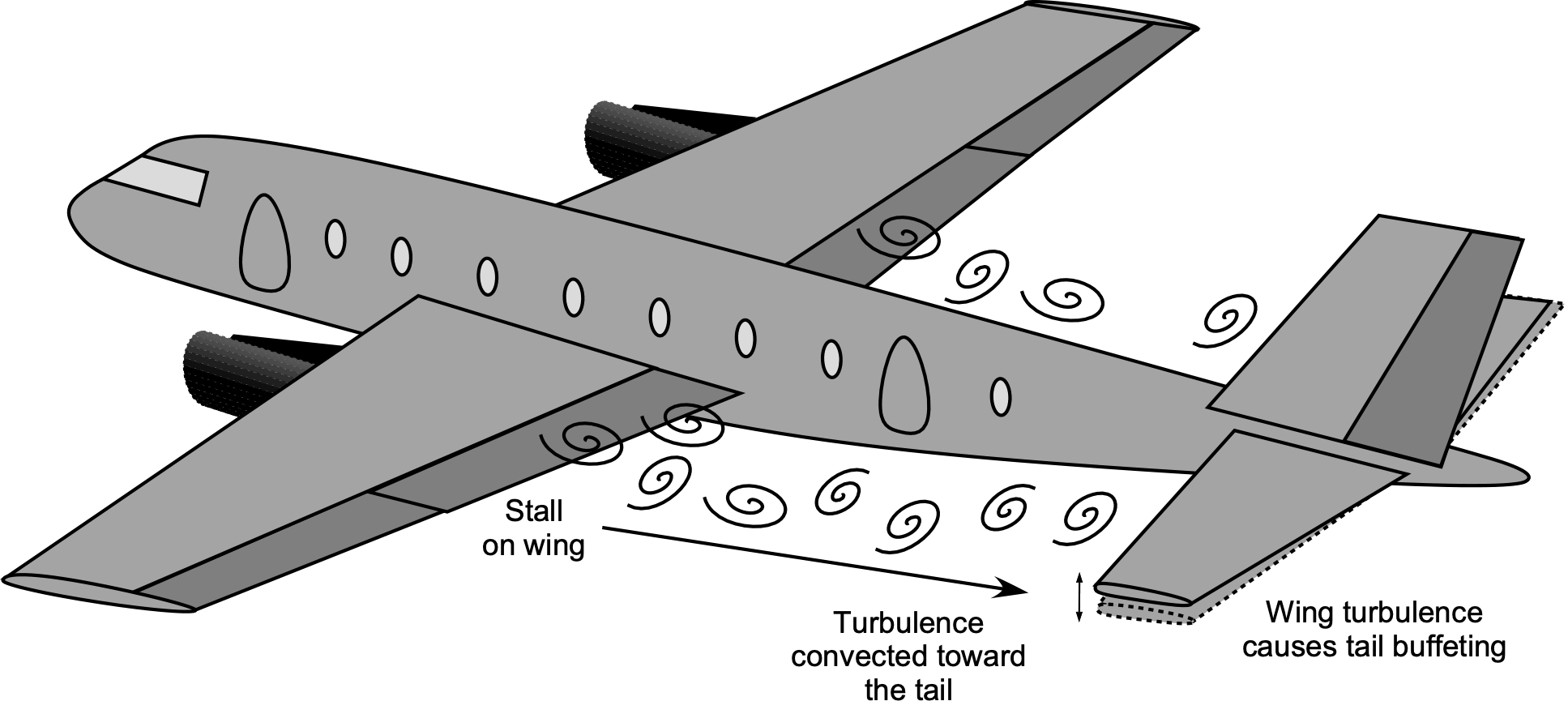
For example, an aircraft’s horizontal stabilizer may experience buffeting when positioned within the wake of the wing or fuselage, as shown in the figure below and this video of the MD-11 airliner stall tests. This behavior may occur at higher angle of attack operations, such as during takeoff or landing, especially when flaps are deployed. Similarly, shock waves interacting with boundary layers in transonic or supersonic flight can induce separated flow regions that produce turbulence and cause severe buffeting on downstream airframe structures.

Buffeting is an essential consideration in airplane design because it can increase aerodynamic drag, lead to control difficulties, and produce structural fatigue. Engineers analyze and mitigate buffeting effects using wind tunnel testing, CFD simulations, and flight testing. Techniques to reduce buffeting include optimizing the shape and size of aerodynamic surfaces, adding vortex generators to reduce or control flow separation, and designing control systems to minimize the response to buffeting forces.

Buzzing

Buzzing is a high-frequency aeroelastic behavior that occurs primarily in control surfaces such as ailerons, rudders, and elevators. It is caused by the interaction between the aerodynamic forces acting on a control surface and the structural dynamics of the hinge mechanism. Unlike buffeting, which is an externally forced vibration, buzzing is a self-excited oscillation resulting from unsteady aerodynamic loading on a lightly damped control surface. A common cause of buzzing is aeroelastic feedback from hinged surfaces, as shown in the figure below.

If a control surface is not sufficiently stiff or damped, small disturbances in the airflow can lead to rapid oscillations of the surface, which aerodynamic forces may then amplify. In transonic or supersonic flight, buzzing can also result from shock-induced separation and reattachment over a control surface. This creates fluctuating pressure loads that drive high-frequency shock wave strength and location oscillations. Engineers can mitigate buzzing by adding stiffness, mass balance weights, or dampers to suppress these rapid and undesirable control surface movements.

Summary & Closure

In aeroelastic analysis, engineers study phenomena such as flutter, divergence, and other dynamic instabilities that affect airplane structures. Mitigating these effects is crucial for designing wings, control surfaces, and other components that can withstand aerodynamic forces while maintaining stability and performance throughout the flight envelope. A deep understanding of aeroelasticity ensures modern aircraft remain “flutter-free” and meet stringent safety and performance standards under all flight conditions.

With the advent of powerful computers and advanced numerical methods such as FEM and CFD, aeroelastic modeling has become highly sophisticated. Modern software tools enable detailed simulation of aeroelastic phenomena, including flutter, divergence, and control reversal. These tools are used extensively in the design of modern aircraft and spacecraft. Aeroelasticity has become a mature field that integrates advanced computational techniques with experimental methods to ensure the safety and performance of all aerospace flight vehicles.

5-Question Self-Assessment Quickquiz

For Further Thought or Discussion

What are the key differences between static and dynamic aeroelasticity? Can you provide examples of each?
Why is divergence considered a catastrophic failure mode, and how can it be prevented in modern aircraft design?
What role might composite materials play in controlling aeroelastic effects in modern aircraft design?
Identify a historical aircraft accident that resulted from aeroelastic effects. What lessons were learned?
How did the introduction of swept-wing designs impact the aeroelasticity of jet aircraft?
How might controlled aeroelastic effects be intentionally used to enhance aircraft performance rather than being just a constraint?
How might aeroelasticity impact the design of wind turbines? Hint: Do not limit your discussion just to the turbine blades.

Other Useful Online Resources

Visit the following websites to learn more about the phenomenon of flutter:
Aeroelasticity – Introduction to Flutter.
Aerospace Structures – Aeroelasticity.
Video showing the process Airbus follows with flutter testing.
Can we make commercial aircraft faster? Mitigating transonic buffet with porous trailing edges.

Named after Arthur Roderick Collar, who worked extensively on aeroelasticity. ↵
At least initially, but this issue was soon rectified as flutter became better understood. ↵
The inclusion of the zero "0" in F0VMS is deliberate. ↵
And under all the same assumptions as the classic thin airfoil theory. ↵
The terms "noncirculatory" or "apparent mass" or "added mass" are often used synonymously. ↵
Theodorsen, T., "General Theory for Aerodynamic Instability and the Mechanism of Flutter," NACA TR 496, 1935. ↵
Notice that this case does not represent an oscillating airfoil because the pitch-rate terms are not included. ↵
This means that aerodynamics adjust instantaneously to changes in pitch angle with no time lag, even though this is physically incorrect for higher reduced frequencies. ↵
The design was modified by adding additional structural reinforcements to ensure flutter-free operation. ↵

License

Icon for the Creative Commons Attribution-NonCommercial-NoDerivatives 4.0 International License

Introduction to Aerospace Flight Vehicles Copyright © 2022–2025 by J. Gordon Leishman is licensed under a Creative Commons Attribution-NonCommercial-NoDerivatives 4.0 International License, except where otherwise noted.

Introduction

History

Unsteady Airfoil Behavior

Reduced Frequency

Quasi-Steady Aerodynamics

Apparent Mass Terms

Quasi-Steady Aerodynamics, Including Apparent Mass

Frequency Domain – Theodorsen’s Theory

Governing Equation

Theodorsen Function

Aerodynamic Response

Time-Domain – The Indicial Response

Non-Dimensional Time

Wagner’s Problem

Discretization of Duhamel Integral

Aeroelastic Analysis

Torsional Flutter of a Cantilevered Wing

Analytical Approach to Flutter

Time-Marching Solution

Flutter of a Two-Dimensional Airfoil Section

Flutter Speed Determination Using Theodorsen’s Function

Flutter Using FEM/CFD Coupling

Flutter Occurences in Practice

Flight Control Reversal

Dynamic Stall & Stall Flutter

Dynamic Stall

Stall Flutter

Buffeting & Buzzing

Buffeting

Buzzing

Summary & Closure

License

Share This Book