44 Aircraft Propellers
Introduction
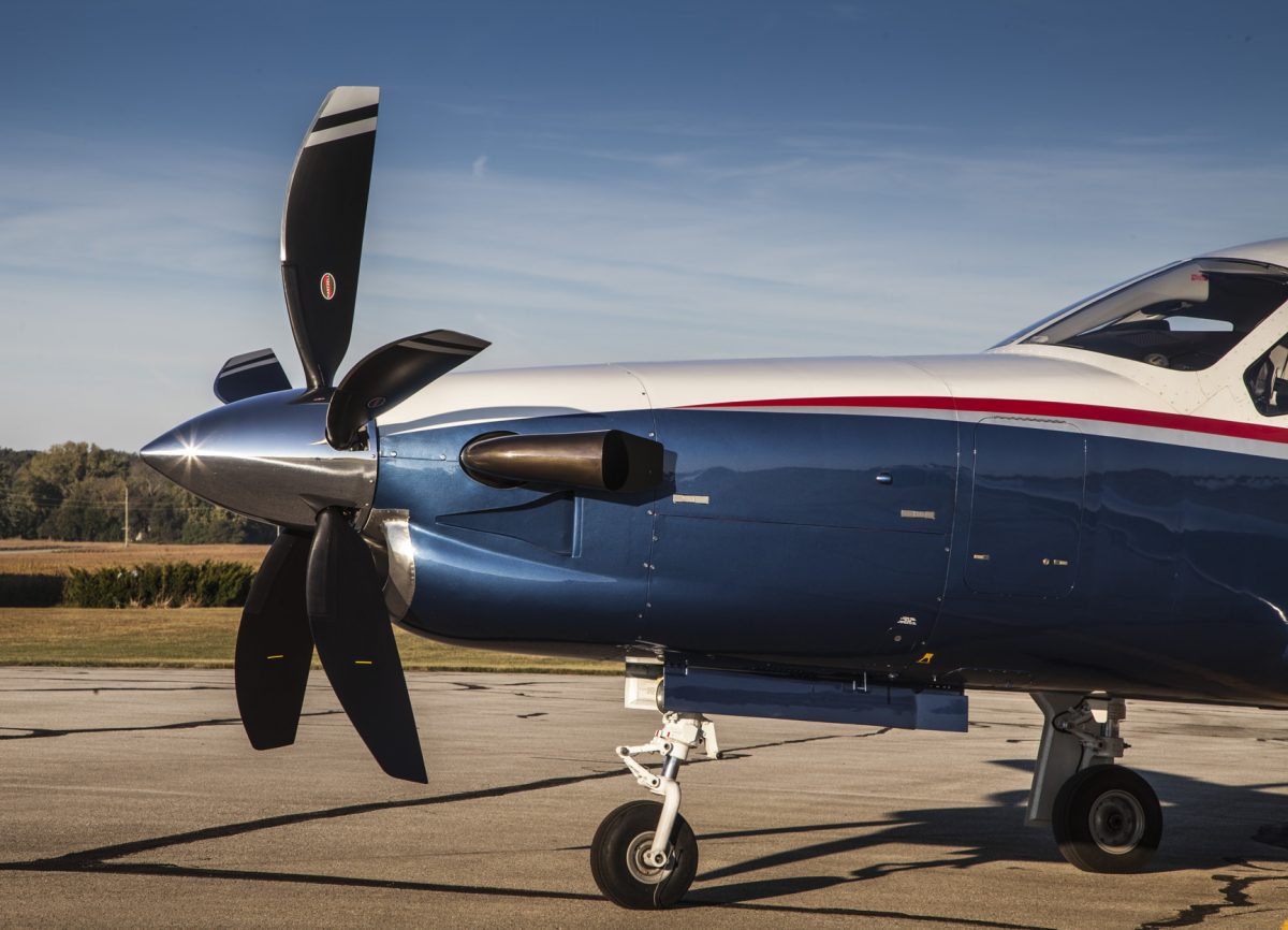
The modern propeller stands as a testament to the achievements of aeronautical engineering. Since the earliest days of flight, propellers have been the focus of continuous refinements and technological advancements, further shaping the evolution of aircraft designs. Today, companies such as Hartzell, Sensenich, and McCauley produce highly efficient, advanced propellers made of composite materials, aerodynamically optimized airfoil sections, and sophisticated blade geometries with swept leading edges to minimize compressibility effects. These modern designs, exemplified by the photograph below, reflect more than a century of progress in aerodynamics, materials science, and manufacturing techniques, closely paralleling and often driving broader innovations in aviation.
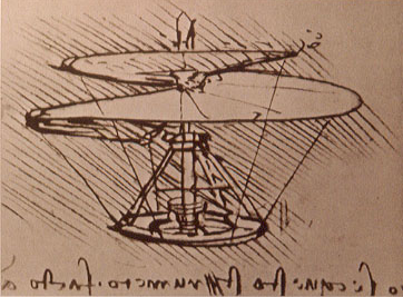
The earliest known use of propellers or rotors dates back to around 500 BC in ancient China, where children played with bamboo dragonflies. These were simple wooden toys consisting of a stick and blades that, when spun rapidly between the hands, would lift into the air. Leonardo da Vinci, in the 1480s, sketched the “aerial screw,” as shown in the figure below. This concept was an aerodynamic device derived from an Archimedes water screw, which some consider a precursor to the modern helicopter rotor. Although never built at its intended human-carrying scale,[1] Da Vinci’s design laid down the concept of using rotating wings to create an aerodynamic force parallel to their axis of rotation, a force called thrust.
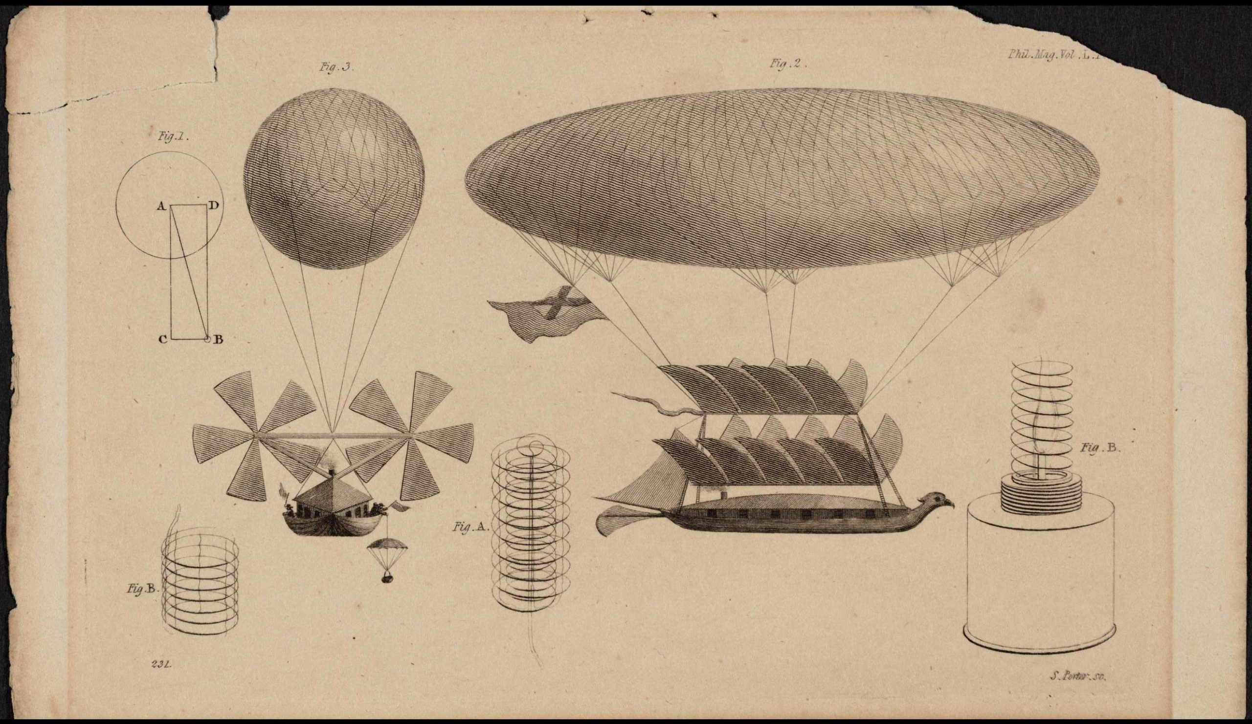
In the 19th century, George Cayley made significant contributions to understanding the principles of flight, experimenting with gliders and recognizing the need for a powerplant and propulsion mechanism if sustained flight was ever to be achieved. At least one of his airplane concepts and an airship, the latter shown in the illustration below, indicated that the means of propulsion was using “airscrews” or propellers. The power source was not specified, although the only option at the time would have been a steam engine.[2] The use of “screw” propellers for propulsion was nothing new, having been used in marine applications since the 1830s. Still, the propeller blade designs suitable for good efficiency in the air had yet to be determined. In the 1870s, Thomas Moy built the Aerial Steamer, an early powered aircraft with two, six-bladed propellers driven by a steam engine. The blades had geometric twist, their pitch becoming finer at the blade tips. Like the Cayley concept, however, although it did not fly, it was a step forward in critical thinking about how an airplane might be propelled.
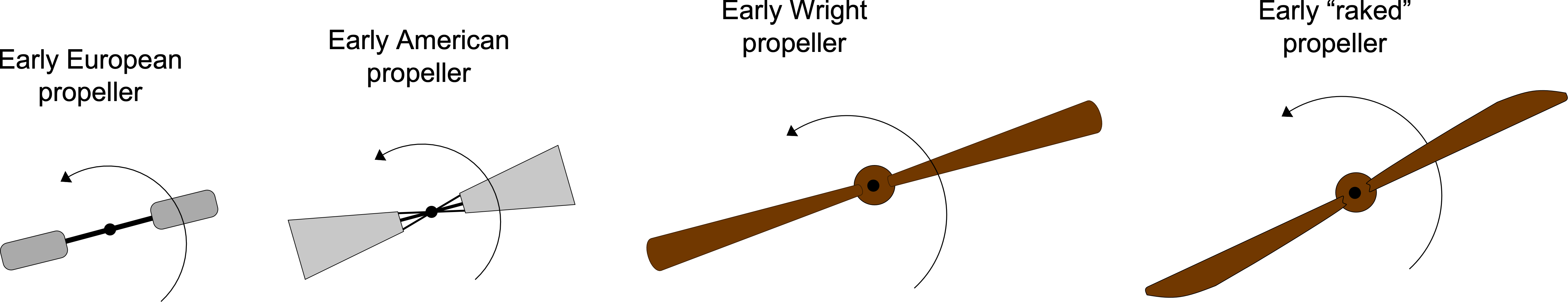
In 1903, the Wright brothers made the first successful, powered flight with their Wright Flyer, equipped with twin wooden propellers designed and built in their workshop. The Wrights discovered that there was no theory or other analysis to describe or predict propeller performance. The state of the art at the time was simply trial and error. They then set out to study the aerodynamics of propellers in a wind tunnel of their own design, demonstrating that long, thin (i.e., high-aspect-ratio) blades with nose-down twist (called washout) along their span yielded the best propulsive efficiency. By 1908, they had improved their propeller designs for the Wright Flyer III, enabling flights of much longer duration and range. Their “raked” propeller had a swept leading edge and more blade area toward the tip, as shown in the figure below. This design gave further efficiency improvements, allowing more of the limited engine power to be converted into thrust. The broader propeller tips were also structurally stiffer, preventing them from buzzing and fluttering, a shortcoming of many early propeller designs.
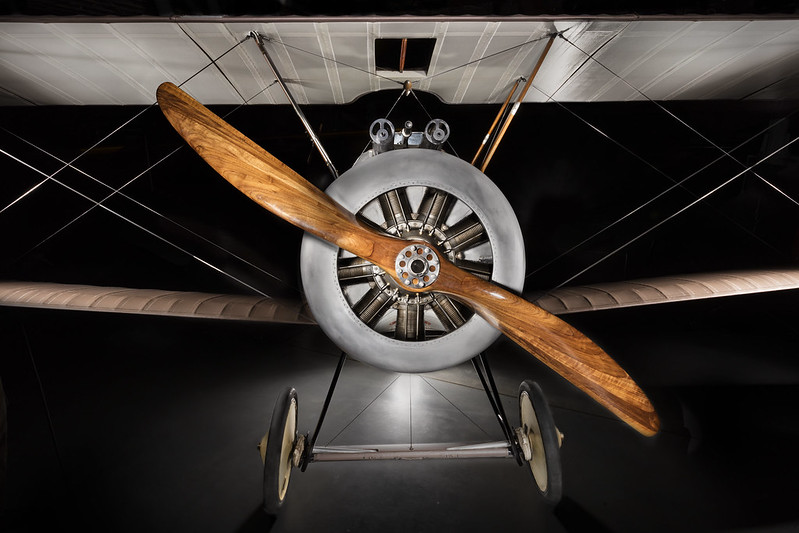
During WWI, propeller technology advanced rapidly to meet the demand for airplanes with greater performance. Initially, fixed-pitch wooden propellers carved from laminated spruce blocks were standard, as shown in the photograph below. However, as engine power and aircraft speeds increased, the limitations of wooden propellers quickly became evident, including cracking and delamination. They were also very vulnerable to damage in combat, with a single bullet through a wooden blade often causing its catastrophic failure.
While wood was easy to work with and, with sufficient skill, propellers could be carved to almost any shape, the quest for more durable propellers led to metal blades, initially made of steel. Steel offered significantly greater strength and resistance to damage, though it introduced additional challenges, such as increased weight and the need for more complex, expensive manufacturing processes. One of the earliest airplanes using steel propellers was the Handley Page O/400 bomber, which significantly improved its flight performance and reduced its vulnerability in the demanding conditions of long-range bombing missions under enemy fire.
With the formation of dedicated research institutions, such as the NACA and the Royal Aircraft Establishment (RAE), the aerodynamic principles governing propeller performance began to be systematically quantified. From the 1920s to the 1950s, NACA conducted wind tunnel tests and collated detailed data on propeller performance. Engineers experimented with various blade planforms, including tapered and hyperbolic shapes, as well as specific tip shapes and airfoil sections better suited to propellers. The RAE also researched propellers extensively, focusing on theoretical aerodynamic analyses, mainly by Hermann Glauert[3], supported also by wind tunnel measurements. These propeller developments laid the groundwork for more sophisticated airplane designs, contributing to the rapid evolution of aviation technology.
Materials like duralumin, an aluminum alloy invented in the mid-1920s, were used to make propellers lighter and stronger. Engineers soon began developing variable-pitch aluminum propellers, allowing pilots to adjust the blade pitch angles for optimal flight performance. This significantly improved propeller efficiency and airplane performance over a broader range of airspeeds. In the 1930s, Hamilton Standard introduced the first controllable pitch propeller. During takeoff and climbout, the pilot could use a lower blade pitch for optimal performance, then shift to a higher blade pitch for efficient cruising. This innovation soon led to the constant-speed propeller, which automatically adjusted blade pitch during flight using a governor [4] to maintain a constant rotational speed and continuously maximize the propeller’s propulsive efficiency.
. Studio photograph in support of \"Pioneers of Flight\" exhibit")
During WWII, propeller-driven aircraft technology reached new heights, with significant advancements in propeller design, aerodynamics, engine efficiency, structural reliability, and overall weight reduction. The introduction of propellers with more blades was another crucial development. Initially, two-blade and three-blade propellers were standard. Still, engineers soon realized that four-blade and five-blade designs were needed to absorb the power from increasingly powerful piston engines. Additional blades also provided smoother operation, reducing vibrations from the engine and propeller, and improving the airplane’s overall performance at higher airspeeds. As engine power levels increased further after the advent of supercharging and turbocharging, counter-rotating tandem propellers were used to prevent a single propeller from becoming prohibitively large and thereby absorbing all available engine power.
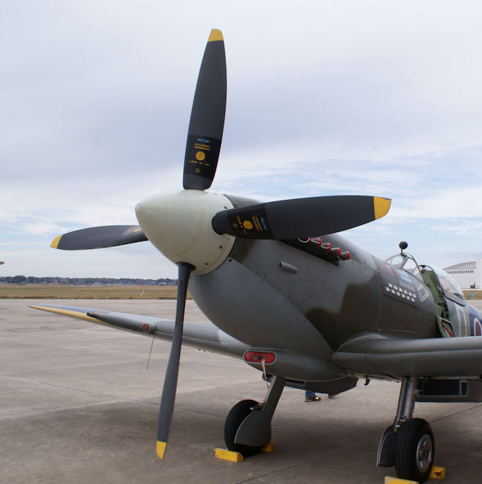
Iconic WWII aircraft, such as the British Supermarine Spitfire and the American North American P-51 Mustang, exemplified advancements in propeller and engine technology. The Spitfire, with its powerful Rolls-Royce Merlin engine and Rotol four-bladed aluminum propeller design, as shown in the photograph below, achieved exceptional performance in terms of achievable airspeeds and operational altitude. Later models of the Spitfires were equipped with a five-bladed propeller powered by a version of the Rolls-Royce Griffon engine, representing the pinnacle of piston-engine and propeller performance. The P-51 Mustang, when fitted with a four-bladed Hamilton Standard propeller, became renowned for its long flight range, speed, and effectiveness as an escort fighter.
These technological improvements in propeller design were also applied to bombers and transport aircraft, such as the Boeing B-17 Flying Fortress, the Consolidated B-24 Liberator, the Avro Lancaster, and the Douglas C-47. Propellers played a crucial role in improving the speed, altitude, and range of these aircraft, ultimately contributing to the Allied victory in WWII. The increased efficiency and reliability of propeller-driven airplanes enabled more effective long-range bombing campaigns, strategic airlift, and supply missions. Additionally, advancements in aerodynamics and engine integration enabled these aircraft to carry heavier payloads while maintaining maneuverability and endurance in combat operations.
The transition to using gas turbine (turbojet) engines after WWII soon surpassed the use of propellers in most military and commercial aviation. Nevertheless, propeller technology continued to evolve for specific applications, including high-speed fighter airplanes. However, the most significant interest in new propeller developments was in turboprop engines, which used a turboshaft to drive a propeller, offering high propulsive efficiency at lower speeds and altitudes than pure jet engines. This advancement made turboprop “jet” airliners ideal for shorter routes where fuel efficiency and short takeoff and landing capabilities, such as at regional airports, were critical.
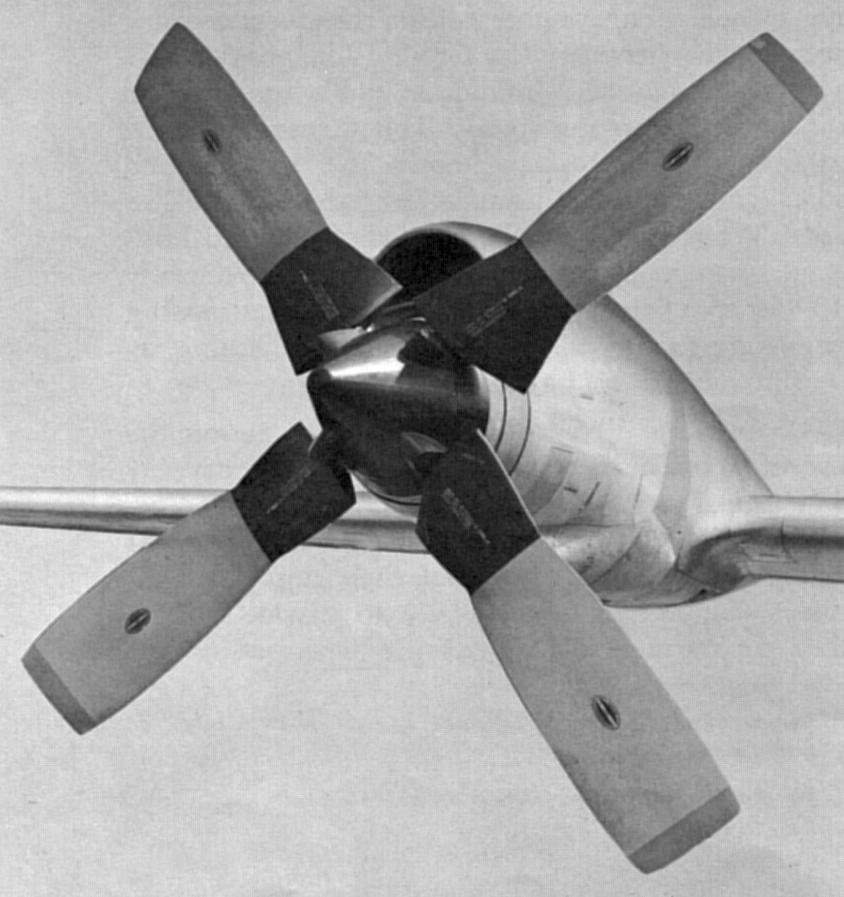
The Lockheed L-188 Electra, which entered service in 1958, demonstrated the enduring significance of propeller-driven airplanes; one of its four-bladed propellers is shown in the photograph below. Airplanes like the Lockheed C-130 Hercules, the modern Airbus A400M Atlas, and the C-130J Super Hercules have since leveraged advances in turboprop technology to improve their efficiency, versatility, and reliability. Today, the turboprop remains a preferred propulsion system for many airplanes and can be found on high-performance single-engine aircraft, such as the Pilatus PC-12 and the Cessna Caravan 208.
While the basic engineering principles used in aircraft propeller design have remained unchanged for decades, numerous detailed improvements have led to continuous gains in propulsive efficiency and operational reliability. Propeller construction methods have continued to advance, using carbon and graphite composites to produce lighter, more aerodynamically efficient blades with reduced noise. Engineers continue to use techniques such as computational fluid dynamics (CFD) and computer-aided design (CAD) to further optimize propeller performance, tailoring them to specific engines, aircraft, and flight conditions.
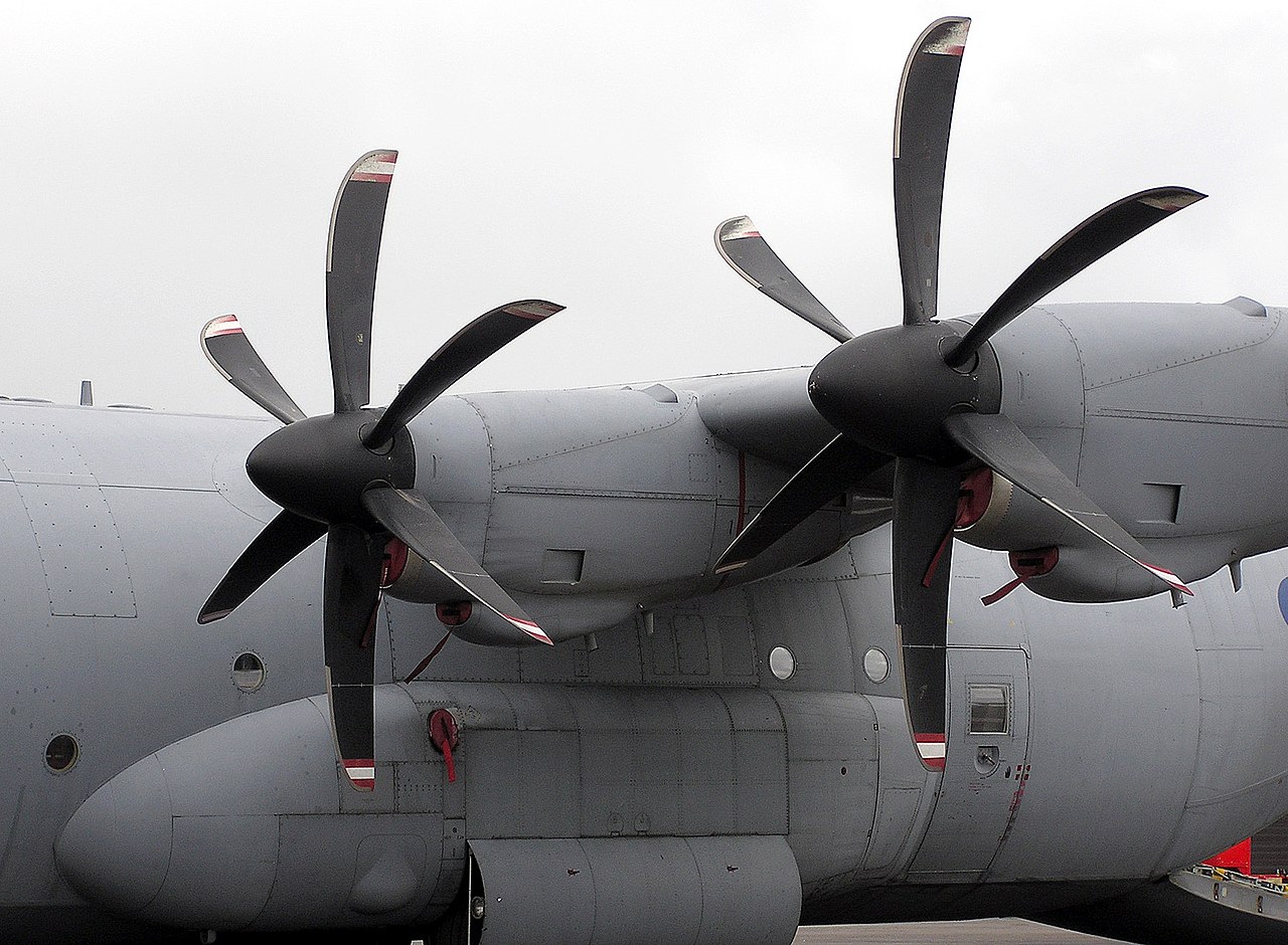
Most modern propellers feature swept leading edges and thin airfoil sections, as illustrated in the photograph below. Scimitar propellers, which have highly swept blades made primarily of composite materials, were developed in the 1980s. Like the swept wings used on high-speed aircraft, these propeller blades delay the onset of drag rise and wave drag, allowing them to remain efficient propulsors at higher flight speeds and Mach numbers. They also reduce noise, a significant concern for all modern aircraft due to increasingly stringent ICAO noise standards. This swept-blade propeller design is used in many modern turboprop aircraft, including the ATR 72, Bombardier Dash 8, and Pilatus PC-12.
Ongoing developments in propeller designs for electrically powered airplanes focus on improving efficiency and reducing noise, particularly for urban air mobility (UAM) and unoccupied aerial vehicles (UAVs). Engineers are exploring innovative blade geometries and lightweight materials to create quiet, compact propeller systems that meet the unique demands of drones, electric airplanes, and eVTOL concepts. The goals include optimizing flight performance with multi-rotor systems and variable-pitch propellers, while leveraging advances in battery technology and manufacturing techniques. While the tipping point in favor of electric propulsion over traditional approaches is likely decades away, technology developments are progressing rapidly.
Learning Objectives
- Have an appreciation of the historical developments of propeller technology from the days of the Wright brothers to the present.
- Understand the basic operational principles of a propeller, including the methods used to calculate its thrust, the power required, and its efficiency.
- Be familiar with momentum theory and blade element theory when calculating the performance of a propeller.
- Know how to read and interpret a propeller performance chart.
- Understand the operational advantages of variable-pitch propellers compared to fixed-pitch designs.
- Know how to select a propeller to meet a performance requirement, including for low-Reynolds-number propellers.
Propeller Fundamentals
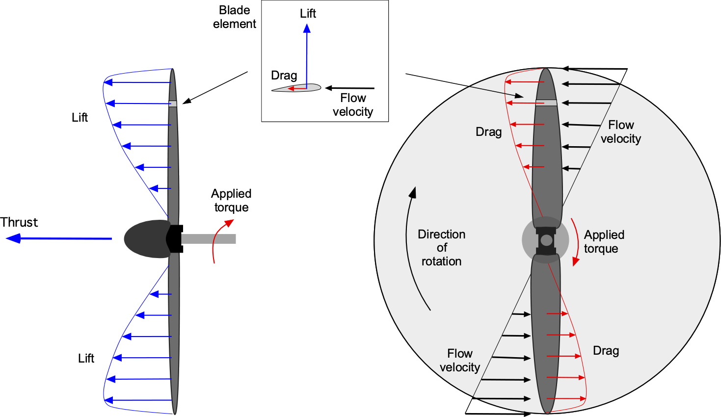
Propellers convert rotational motion into thrust by creating aerodynamic lift forces on their blades, which act as rotating wings. As the blade moves through the air, the airfoil’s shape creates an aerodynamic pressure difference between the upper and lower surfaces, generating lift. The resolved forward component of the lift vectors is known as the propeller’s thrust. The engine supplies torque to the propeller shaft, which, in turn, overcomes the drag forces on the blades and maintains their rotation. Sedulous propeller design maximizes thrust by optimizing blade geometry, angle of attack distribution, and rotational speed, ensuring that the engine’s power is converted into propulsive force with maximum efficiency.
Velocity Triangle & Blade Twist
A notable design feature of propeller blades is their significant twist along their span, i.e., geometric washout. Each blade is composed of an airfoil section. Because of the variation of flow velocity along the blade, the twist ensures that the local angle of attack at each section remains near its most aerodynamically efficient value across the entire blade span. In practice, most sections should have angles of attack between about  and
and  , or otherwise near their angle of attack for the peak lift-to-drag ratio, i.e.,
  . The result is maximum thrust production for minimum torque and shaft power.
To understand why a propeller blade must be significantly twisted, consider the following analysis. Let  be the radius of the propeller and let
  be the spanwise distance from the axis of rotation to a blade element, as shown in the figure below. The corresponding nondimensional radius is
  , and the root cutout, which is aerodynamically passive, is
  . The angular velocity is
  , and the tangential (in-plane) velocity increases linearly with , i.e.,
  . The local geometric blade pitch angle,
  , is defined relative to the plane of rotation.
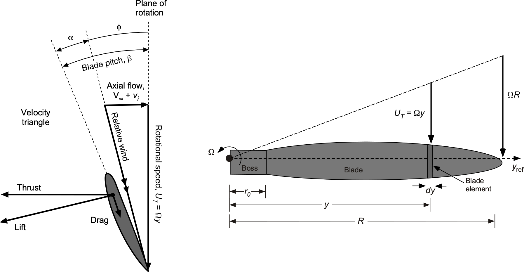
Assume that the axial velocity  through the propeller disk is uniform, such that
  . The total relative velocity (also known as the relative wind) at the blade section
  is then
(1) 
The inflow angle is
(2) 
and so the sectional angle of attack is
(3) 
Notice that the axial velocity is the sum of the freestream velocity (airspeed)  and the induced velocity
  , i.e.,
(4) 
For a propeller in its normal working state during flight,  , whereas for static thrust (hover)
  , so that
  . In either case, is assumed to be uniform across the propeller disk, consistent with the Rankine-Froude actuator disk assumption, which is also a design goal to minimize losses.
Under the assumption of a constant aerodynamic angle of attack, i.e., , it follows that
(5) 
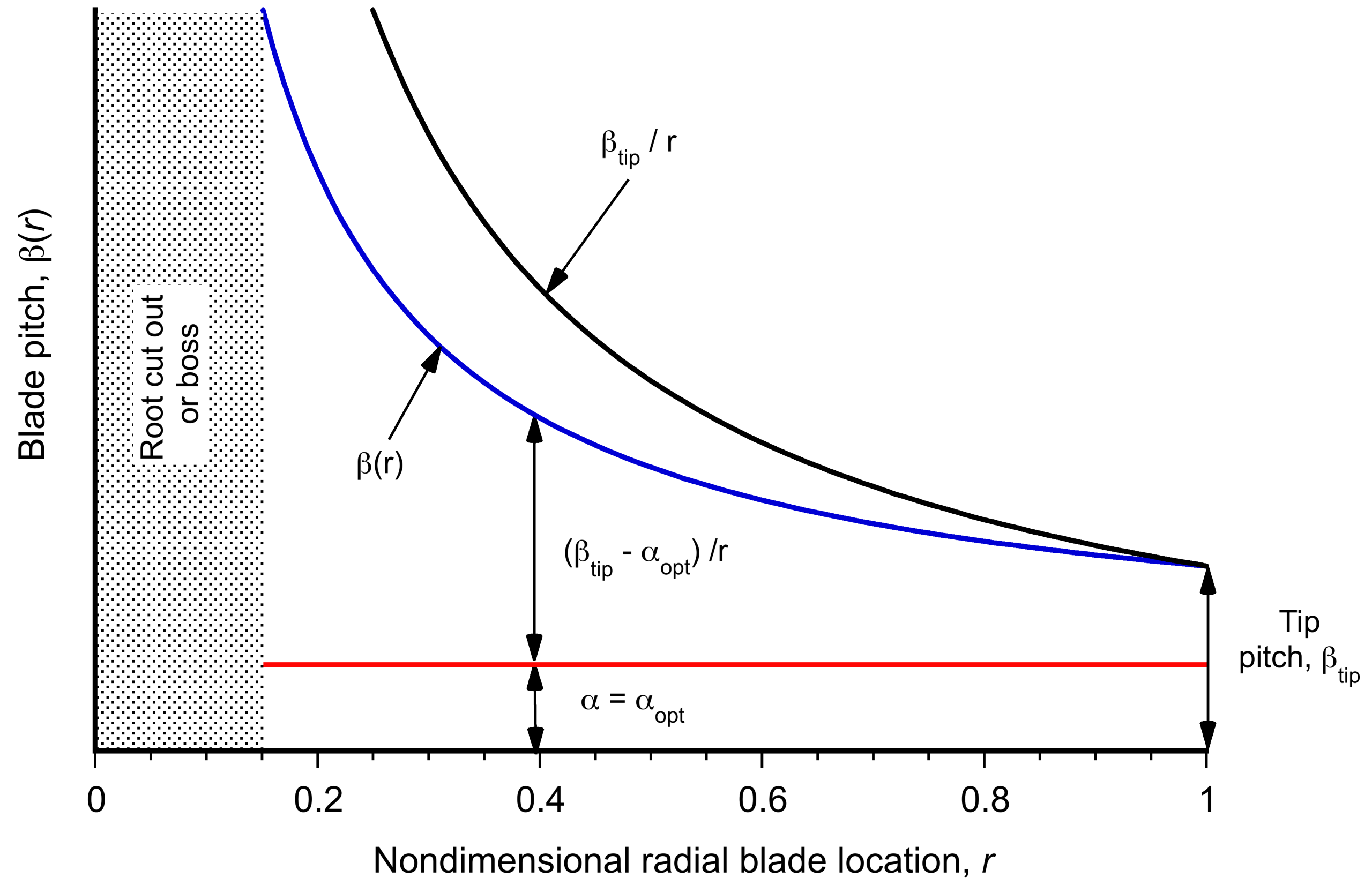
which suggests a canonical form for the twist distribution, i.e.,
(6) 
because  is a constant. This expression shows that must follow a hyperbolic variation proportional to
  , i.e., in general
(7) 
as shown in the figure below. The twist angle is larger near the root and decreases toward the tip, thereby ensuring a constant angle of attack along the blade span. However, because of the variations in Mach number, Reynolds number, section thickness-to-chord ratio, and camber (i.e., zero-lift angle of attack,  ), the best angle of attack is not necessarily a constant. The net twist will vary for different propellers based on their intended application, but the net washout angles may be as large as 40 degrees over the blade span; of course, these twist angles are significantly larger than those used on airplane wings.
Fixed-Pitch Versus Variable Pitch
Fixed-pitch propellers have a narrow operating envelope; they are either suitable for takeoff and climb but perform poorly in cruise, or they are suitable for cruise but perform poorly in takeoff and climb. This is because at higher airspeeds, the blade section angles of attack on a propeller of fixed pitch will become progressively smaller, so the propeller produces progressively less thrust. The solution to this dilemma is to change the average blade pitch angles[5] to maintain or increase thrust production and allow the efficient operation of the propeller to be optimized as a function of the flight condition, the idea being shown in the figure below.
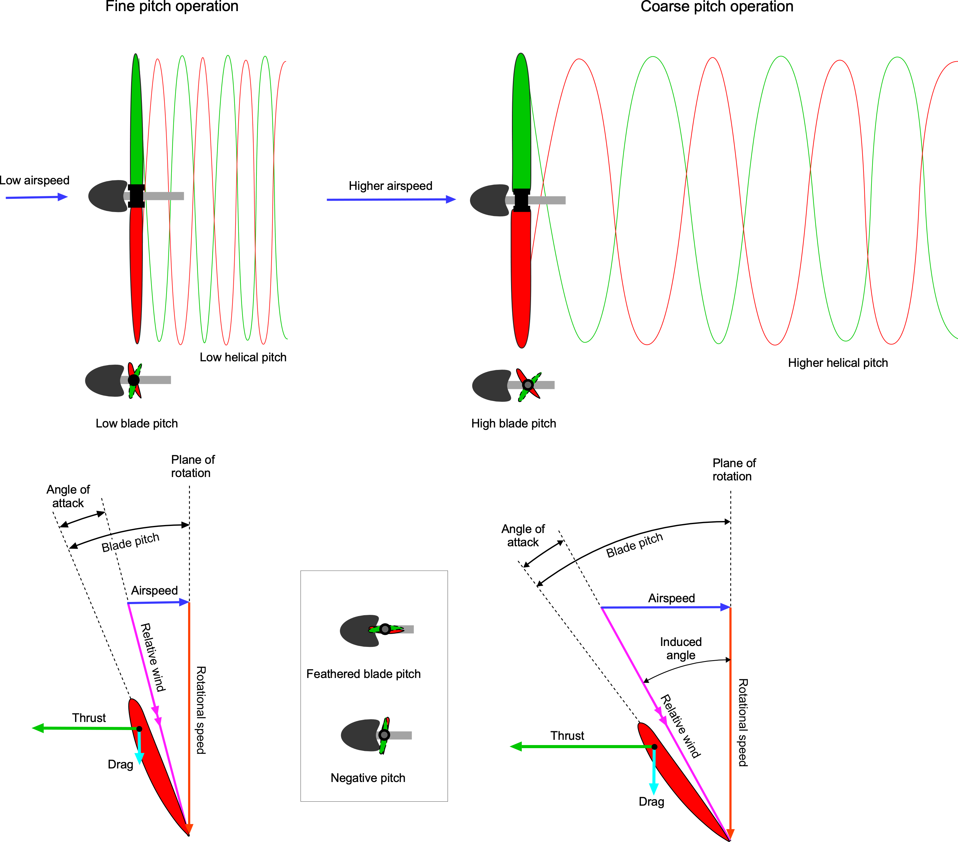
To maximize thrust and propulsive efficiency, a fine (low) blade pitch will be used for takeoff and landing, and a coarser (higher) blade pitch will be used for cruise flight. Regulating the blade pitch angles in this manner optimizes the propeller’s efficiency as a function of flight condition. Therefore, an aircraft equipped with a variable-pitch or constant-speed propeller can maintain high thrust and propulsive efficiency over a broader range of airspeeds. In cruise flight, a speed governor can automatically adjust the blade pitch to maintain the propeller’s constant rotational speed, thereby offloading much of the pilot’s workload for controlling the propeller pitch.
The highest thrust from the propeller will be limited by the onset of stall, just as a regular wing is limited in its angle of attack capability by stall. However, because the local incident Mach number varies from the root to the tip of the propeller, and the stall angle of attack of an airfoil decreases with increasing Mach number, the allowable angle of attack before stall decreases from the root to the tip. To this end, thin airfoil sections with higher lift-to-drag ratios and higher drag-divergence Mach numbers are used. However, the onset of stall will eventually occur if the blade pitch is increased too much, accompanied by a loss of thrust, an increase in power, and a marked drop in propulsive efficiency.
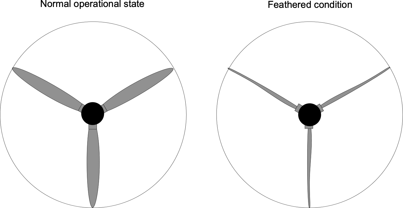
If the engine stops in flight, the propeller blades must be “feathered” into the airflow to reduce the otherwise high drag of the stationary blades. This means the leading edges of the blades will point almost directly into the airflow, as shown in the figure below. In this regard, strong springs are used on a constant-speed propeller so that the blades are automatically forced into the fully feathered position if the propeller stops rotating. The drag of an unfeathered stationary propeller is considerable, so an airplane with a fixed-pitch propeller will inevitably have a poor glide ratio. The propeller blades may sometimes be set to a negative pitch to produce negative thrust, thereby acting as an aerodynamic brake during landing. However, this latter feature is usually found only in high-performance turboprop aircraft.
Types of Propellers
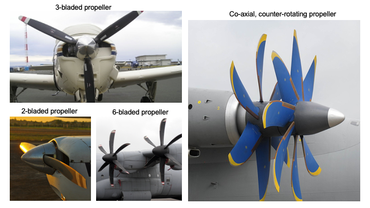
Many propeller types are in use, ranging from those with just two blades to those with four or more blades, some with fixed pitch and others with variable pitch, as shown in the photographs below. In addition, some propellers may have swept blades, a design feature that reduces compressibility drag at the tips when the airplane operates at higher flight speeds, similar to the design used on the wings of supersonic airplanes. As engine power increases, more blades (or a greater blade area) are required to deliver the power to the air as useful thrust. In some cases, to prevent the propeller diameter from becoming too large, counter-rotating propellers may be used to absorb the high power available from the engine shaft and generate thrust.
Propellers with more blades tend to be relatively more efficient (when compared at the same thrust and total blade area) because they act more like an actuator disk.[6] However, the propeller’s net efficiency depends on other factors, including operating speed (rpm or rps),[7] tip Mach number, blade section Reynolds numbers, diameter, and blade pitch. Today, there is an increasing emphasis on reducing propeller noise, which has driven engineers of modern designs (even on general aviation airplanes) to use more blades and smaller diameters with lower tip Mach numbers.
What is the difference between propeller power and torque?
Torque, given the symbol  , is the rotational action applied to the propeller shaft, while angular velocity, , is the speed at which the propeller rotates, measured in radians per second. Power,
  , represents the rate at which energy is transferred and is given by the equation
  . A high torque with low rotational speed results in lower power, whereas a lower torque with high rotational speed can still generate significant power. The key to efficient propeller performance is balancing and to achieve optimal thrust and efficiency across different flight conditions. For example, consider a propeller with high torque but lower rotational speed: if = 50 Nm and = 100 rad/s, then the power is = 50
  100 = 5000 W = 5 kW. Alternatively, if the propeller operates at lower torque but higher speed, say = 25 Nm and = 200 rad/s, the power remains the same at = 25 200 = 5000 W = 5 kW.
Momentum Theory of the Single Propeller
The Rankine propeller theory,[8] also known as the Rankine-Froude theory,[9] provides a fundamental framework for understanding propeller performance. This theory models the propeller as an idealized actuator disk that imparts momentum to the air, creating a pressure jump across the disk. The physical problem is that the propeller does work on the air as it passes through the propeller disk; i.e., the propeller applies a force to the air in the downstream direction, changing its momentum and kinetic energy. As a result, the force on the propeller, which is produced because of a pressure difference between one side of the propeller disk and the other, is in the opposite direction to the force on the fluid, i.e., the thrust  is directed upstream.
Flow Model
The flow model for the single propeller problem is shown in the figure below. The upstream and downstream sections labeled 1 and 2 bound the control volume. Remember that when the integral form of the conservation equations is used, then  points out of the control volume by convention. The upstream or freestream (undisturbed) velocity is , and the pressure there is
  . It will be assumed it is uniform, which is a reasonable assumption unless the propeller is affected by a wing or another part of the airframe. It will also be assumed that a one-dimensional, steady, incompressible flow applies throughout, so that the flow velocities change only with downstream distance.
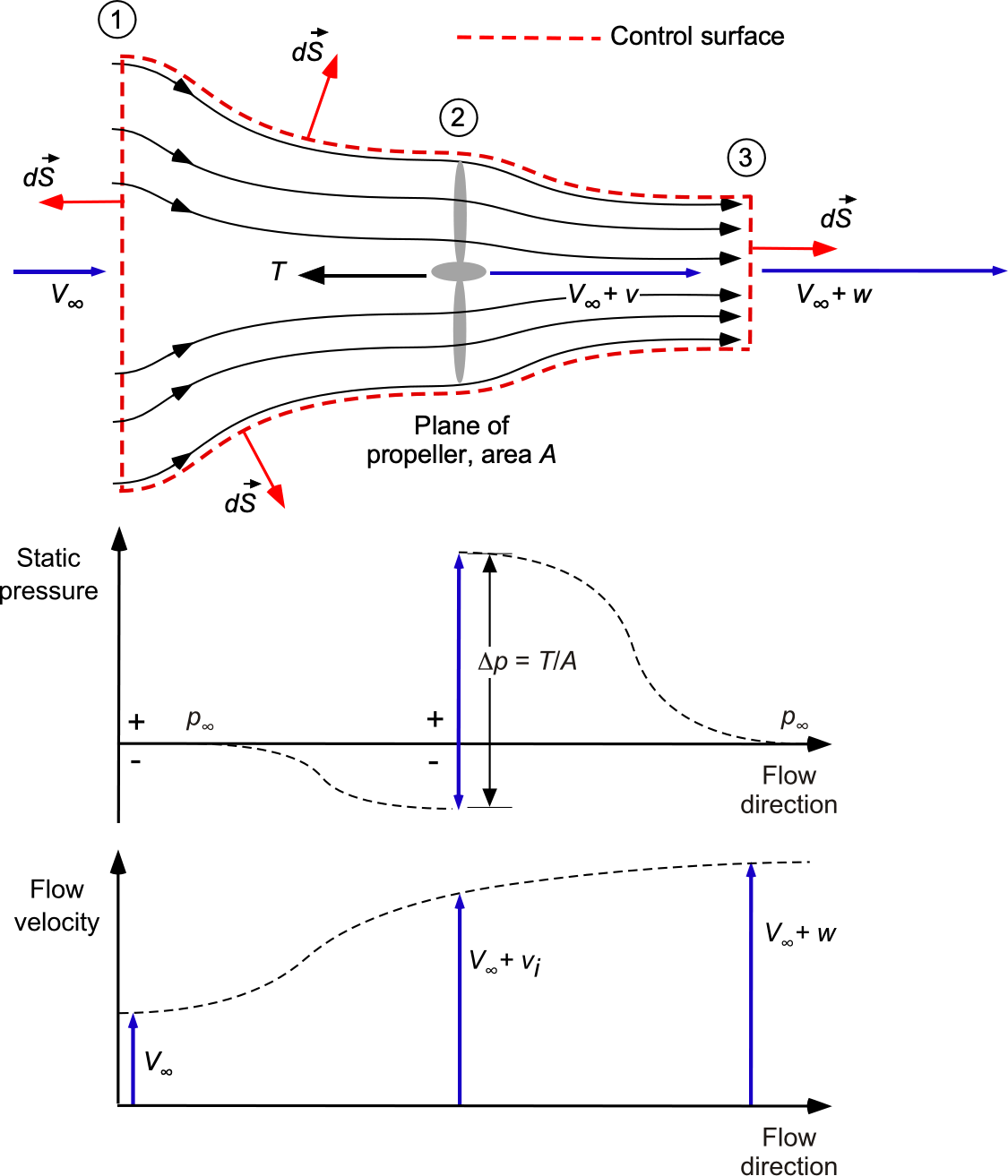
The flow is entrained and accelerated into the propeller, so at the plane of the propeller, the flow velocity is plus an increment  , i.e., the velocity there is
  . The static pressure will also change there. The propeller works on the air to increase its momentum and kinetic energy, so the velocity downstream is
  . In the slipstream, the static pressure will also recover to ambient conditions, i.e., the pressure downstream will slowly return to .
Application of the Conservation Laws
The conservation of mass requires a constant mass flow through the control volume. The areas of the upstream and downstream parts of the streamtube (stations 1 and 2) are unknown, but the area of the propeller disk,  , is known (
 where
where  is the diameter of the propeller), so the mass flow rate through the propeller (and hence through the boundaries of the control volume) is
(8) 
The conservation of momentum requires that the net change in momentum of the fluid (as applied by the propeller) is equal to the force on the fluid, i.e.,
(9) 
where the direction of  is downstream, and the thrust on the propeller, , is in the opposite direction (pointing left in the figure) so that
(10) 
The conservation of energy states that the work done on the propeller (to move it forward) plus the work done on the air (to create the aerodynamic force) must be equal to the gain in kinetic energy of the slipstream as it passes through the propeller, i.e.,
(11) ![\begin{eqnarray*} T (V_{\infty} + v ) & = & \frac{1}{2} \overbigdot{m} (V_{\infty} + w)^2 - \frac{1}{2} \overbigdot{m} V_{\infty}^2 = \frac{1}{2} \overbigdot{m} (V_{\infty}^2 + 2 V_{\infty} w + w^2) - \frac{1}{2} \overbigdot{m} \, V_{\infty}^2 \nonumber \\[6pt] & = & \frac{1}{2} \overbigdot{m} ( 2 V_{\infty} w + w^2) \end{eqnarray*}](https://eaglepubs.erau.edu/app/uploads/quicklatex/quicklatex.com-0e0533aabeb39702be5ef4473a66a55a_l3.svg "Rendered by QuickLaTeX.com")
so that the power required for the propeller to produce the thrust is
(12) 
Notice that the  term on the left-hand side of the above equation can be written as the sum of the
  term, which is the work done to move the propeller forward, i.e., the useful work. The
  term is the work done on the air or the induced power loss; the induced power is an irrecoverable power loss, which constitutes a loss in the propeller’s efficiency in producing useful work.
Induced Velocity
The induced velocity in the plane of the propeller can be found by substituting Eq. 10 into Eq. 12, which gives
(13) 
Expanding out and simplifying gives
(14) 
This result gives the relationship between and  , i.e.,
(15) 
For the next step, take Eq. 10 and substitute in Eq. 8 (mass flow rate) and the connection between and ( ) to get
(16) 
The induced velocity in the plane of the propeller can now be solved for in terms of thrust, i.e.,
(17) 
and expanding out gives
(18) 
The ratio  is called the propeller disk loading. It can be seen that the latter equation is quadratic in
  , which can be solved to get
(19) 
for which there are two roots, i.e., from the  term. Only one can be a physical root (the other one violates the assumed flow model, where the flow is assumed to be through the propeller from left to right), which is
(20) 
(21) 
Therefore, it will be apparent that for any given propeller producing a thrust , its induced velocity will decrease rapidly with increasing airspeeds, i.e.,  . In the design of a propeller in its normal propulsive state, the induced losses can often be ignored compared to the profile losses.
Power Required
The corresponding power required to drive the propeller and produce a thrust, , becomes
(22) 
The useful power for propulsion is , and the second term is the irrecoverable induced loss. Rearranging the preceding equation gives
(23) 
This power equation can also be written non-dimensionally as
(24) 
Notice that in the limiting case when the airspeed, , becomes high, then  , meaning that the induced losses tend to zero. Therefore, a greater fraction of the power delivered to the propeller goes into useful work to propel the airplane forward. However, in practice, some additional profile (non-lifting) power,
  , will be required to overcome the viscous (shear) drag of the blades so that the total power required,
  , can be written as
(25) 
Propulsive Efficiency
The propulsive efficiency of the propeller can also be derived from the preceding analysis. The useful power for propulsion is  so the efficiency of the propeller,
  , can be written as
(26) 
which shows that the propeller becomes more efficient at higher airspeeds, where the induced velocity becomes a smaller fraction of the airspeed. This result also confirms that the efficiency of the propeller at higher airspeeds as  will be dictated by the profile losses on the blades, i.e.,
(27) 
The profile power losses, denoted by , depend on the blade sections and the net blade area, which is measured by the propeller’s solidity or activity factor.
Activity Factor & Solidity
A parameter called the activity factor,  , was used in the earliest days of propeller design. Its definition has originated within the industry rather than in any scientific context. The is considered a measure of the propeller’s “aerodynamic activity” or effectiveness in producing thrust and is defined as
(28) 
where  is the number of blades,
  is the reference chord length of the blade, and is the diameter of the propeller. A higher activity factor indicates that the blades have more lifting area, enabling them to generate more thrust.
Definitions and Nomenclature
Notice that both  and
and  have historically been used to denote the propeller diameter, and they may be used interchangeably. In the NACA literature, the preferred term for diameter is . Similarly, the definition of the reference chord has been inconsistent, ranging from the local chord value at the 70%, 75%, or 80% radius station to a weighted chord based on the platform area distribution. So, it is essential to verify the specific definition used in any given context. Likewise, propeller efficiency may be denoted by
  or , with \ (\ eta_p \) preferred in modern usage.
Solidity, given the symbol  , is a related dimensionless parameter, which is defined as the ratio of the total blade area to the disk area swept by the propeller, i.e.,
(29) 
The scientific literature commonly uses total solidity for the entire propeller and “local” solidity for a specific blade section, which is more geometrically meaningful than the activity factor. The local solidity is given by
(30) 
Notice that a reference or “mean” chord is used when considering total solidity. The most appropriate mean chord for a propeller is a “torque” weighted chord based on
(31) 
where =  and
and  = 0.15 is a starting point or root cutout that accounts for the presence of the propeller hub or “boss.”[10] The reasoning for this
  weighted chord equation is that the blade sections near the tips are much more aerodynamically effective than those near the root end and so more affect the propeller’s performance. In this regard, other definitions of the activity factor have been used, including
(32) 
Therefore, verifying the definitions used when analyzing propeller data in a specific context is essential, especially before conducting any comparative analysis. To be meaningful, the performance characteristics of different propeller blade shapes or numbers of blades, for example, should be performed based on the same value of the activity factor or overall solidity.
Wake Swirl Effects
Incorporating the swirl into the momentum theory involves adding a tangential in-plane velocity component to the otherwise purely axial flow, i.e., a rotational component parallel to the rotor’s plane of rotation. Rankine’s actuator disk theory considers only the axial momentum balance, assuming the flow is steady, inviscid, and incompressible, although Glauert further considered this term. When swirl is included, the average angular velocity component of the downstream flow must be considered, as it affects the power requirements and propulsive efficiency. While the effects are best considered within the framework of blade-element theory, an approximation can be derived from momentum theory.
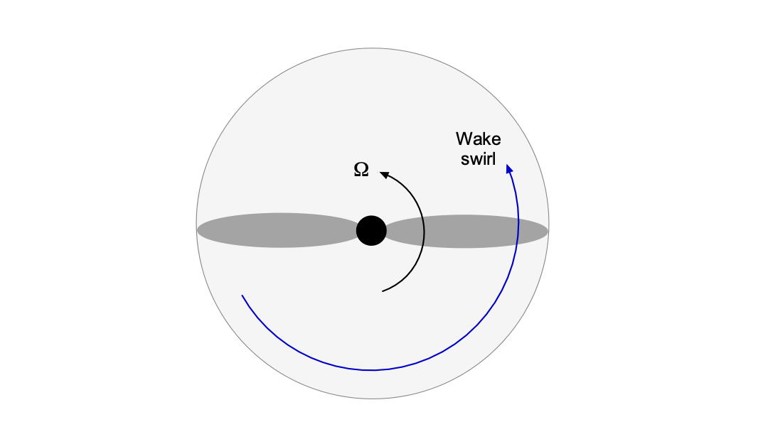
Propeller swirl refers to the rotational velocity of the air in the downstream wake behind the plane of a propeller, which, in effect, creates a spiral or corkscrew flow, as shown in the figure below. This effect occurs because of viscosity, in which the propeller blades drag a certain amount of fluid as they rotate. The upshot imparts a rotational velocity component to the fluid,  , as a consequence of generating thrust. The higher the thrust and torque, the more significant his effect. Swirl causes efficiency losses because some kinetic energy is lost to rotational fluid motion, in addition to that from thrust generation.
Recall that the thrust generated by a propeller with a pure axial velocity component,  , is given by
(33) 
where  is the mass flow rate through the propeller. The power required to generate this thrust, considering the presence of an average swirl velocity, , is
(34) 
where the effective velocity,  , is given by
(35) 
Therefore, the power required is
(36) 
which is greater than the power required for a pure translational change in momentum through the propeller.
In the wake of a propeller, the tangential velocity component, , can be derived from the angular momentum imparted by the propeller blades. The torque, , generated by the propeller can be calculated using the relationship between torque and power, i.e.,
(37) 
where is the power absorbed by the propeller and is the angular velocity of the propeller. The time rate of change of angular momentum, which is a torque, is given by
(38) 
where  is the angular momentum. By using the relationship between torque and angular momentum, the effective radius at which the torque acts can be considered as the mean aerodynamic radius of the propeller, which can be approximated by
(39) 
where is the propeller’s radius (= ). Finally, the average tangential velocity,  , is
, is
(40) 
In practice, the effect of wake swirl on propeller performance is minimal, perhaps reducing the overall propulsive efficiency by 1% to 2%. However, for large propellers driven by high-torque engines, the effects may reach 5%. Coaxial counter-rotating propellers, ducted propellers, and swirl recovery vanes have been employed to mitigate wake swirl and enhance net propulsive efficiency.
Propeller Performance Coefficients
The thrust coefficient for a propeller is a non-dimensional thrust and is defined as
(41) 
where is the thrust generated by the propeller, is the propeller’s diameter, and  is the number of revolutions of the propeller per second (rps). If the rotational angular velocity of the propeller is , then
  . The rotational speed is often measured in revolutions per minute (rpm), so rpm = 60 rps = 60
  .
.
For a propeller, a non-dimensional airspeed called a tip speed ratio or advance ratio, given the symbol  , is defined by
(42) 
Finally, the power coefficient for a propeller is defined as  .
.
Notice that the definitions of propeller thrust coefficient, advance ratio, and power coefficient differ from those used for helicopter rotors. It is essential not to confuse them. The table below clarifies the differences, where = 2.
| Rotating-wing system | Thrust coefficient,  |
Power coefficient,  |
Advance ratio |
| Helicopter rotor |  |
 |
 |
| Propeller |  |
 |
 |
The momentum theory results for a propeller can be written in coefficient form. For the induced velocity, then
(43) 
and for the induced power, then
(44) 
The corresponding propulsive efficiency is then
(45) 
Momentum Theory of the Tandem Propeller
Tandem coaxial propellers are arranged on the same axis but rotate in opposite directions, allowing for a more compact design than separate, non-coaxial propellers. Additionally, the opposing rotation of the propellers cancels out torque reaction effects, which can be very significant when large amounts of power and torque are being transmitted from the engine. In a tandem propeller system, two propellers are aligned along the same axis but operate at different stations, effectively working on the same slipstream. The second propeller acts on the accelerated flow produced by the first, leading to further acceleration and additional thrust.
There are two conditions of interest:
- The rear propeller is sufficiently separated to operate in the slipstream and induced velocity field of the front propeller.
- Both propellers are located so close that they share the same induced velocity.
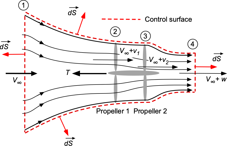
Separated Tandem Propellers
The mass flow rate through both propellers must be conserved for the tandem system, as shown in the figure below. If the first propeller increases the velocity from to  , and the second propeller further increases it to
  , the mass flow rates through each propeller are
(46) 
The thrust produced by each propeller can then be determined, i.e.,
(47) 
The total thrust generated by the tandem system is then the sum of the thrusts produced by each propeller, i.e.,
(48) 
The total power required is the sum of the power required by each propeller, i.e.,
(49) 
The addition of the profile power  is necessary to account for the drag associated with the propeller blades. It affects the overall efficiency of both single- and tandem-propeller systems. The efficiency of each propeller can be expressed as
(50) 
For a tandem configuration with two propellers, the efficiency of each propeller is
(51) 
Therefore, the overall efficiency of the tandem system can then be expressed as
(52) 
Including profile power affects the efficiency calculation because both thrust production and the power required to overcome drag must be balanced. If the profile power becomes significant relative to the thrust generated, it will reduce overall efficiency, particularly at higher speeds where profile losses predominate. In this regard, it will be noted that
(53) 
which is the same result as found for the single propeller, i.e., its net propulsive efficiency mostly depends on the profile power required.
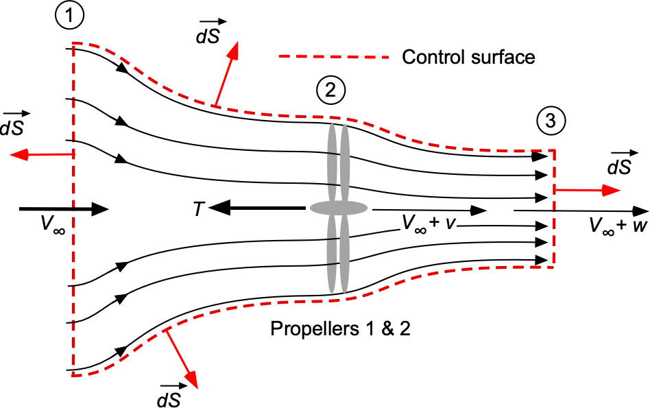
Tandem Propellers with Shared Induced Velocity
Now consider two tandem propellers positioned closely enough to share the same induced velocity increment , as shown in the figure below. The flow velocity at the propeller planes is . The analysis simplifies under the assumption that the induced velocity is the same for both propellers. The mass flow rate through the tandem propeller system is
(54) 
where is the area of each propeller disk, which is assumed to be the same for both propellers.
The thrust generated by each propeller can be expressed as
(55) 
Because both propellers share the same induced velocity , the total thrust is
(56) 
The power required for each propeller is given by
(57) 
and
(58) 
Therefore, the total power required is
(59) 
The efficiency of the tandem propeller system can be analyzed by considering the ratio of useful work to the total power required. The useful work is related to the thrust produced and the forward velocity, . The efficiency of each propeller can be expressed as
(60) 
Incorporating the profile power associated with the drag of the propeller blades, the overall efficiency of the tandem system can be expressed as
(61) 
which again comes to
(62)
Comparing Efficiencies
A common issue in evaluating tandem versus single-propeller designs is the basis for comparison, such as constant net thrust, equal power input, or equivalent solidity, i.e., the ratio of blade area to disk area. Within the framework of momentum theory and its inherent assumptions, no configuration is inherently superior. At higher airspeeds, the profile power required by the blades becomes the dominant factor in determining net propulsive efficiency. Although counter-rotating propellers can recover some energy from wake swirl, this effect contributes only marginally to overall efficiency. It is rarely significant enough to favor one configuration over the other.
When comparing propulsive efficiencies, it is essential to account for the added complexity of managing power distribution between propellers, as well as the overall weight efficiency of the propulsion system. Depending on the specific design choices and operating conditions, a tandem propeller system may outperform or underperform relative to a well-optimized single propeller. The primary advantage of a tandem configuration is its ability to deliver the same power as a single large propeller while using a smaller overall diameter. Ultimately, the effectiveness of any propeller system depends on careful design and optimization to meet the required performance goals, subject to constraints such as size, weight, and cost. Generally, more blades result in higher weight and increased costs.
General Propeller Performance
A more accurate way to predict a propeller’s performance is to use blade-element theory, which can also aid in designing propeller blades for optimal efficiency. Developing a computer program to calculate propeller performance using the blade-element method is a relatively straightforward task. The principle used here is calculating the angle of attack and the corresponding lift and drag at each propeller blade section, as shown in the figure below. All blades are twisted along their span from root to tip, which is done to achieve good aerodynamic efficiency. Therefore, the local blade pitch varies from point to point along the span.
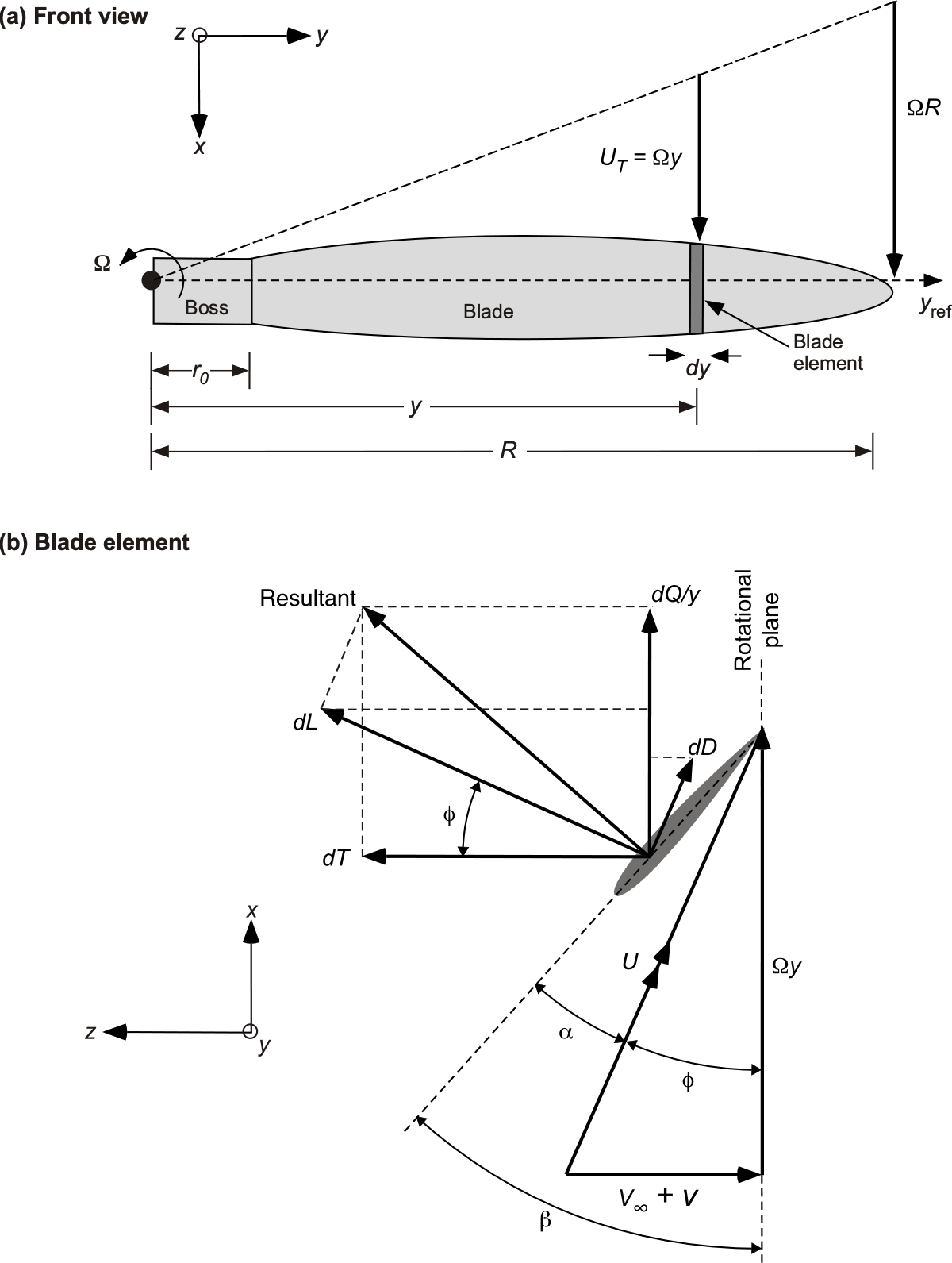
Notice that the relative flow angles and, hence, the angle of attack of the blade element are obtained by using the vector addition of the relative velocity components, i.e., the vector sum of the rotational velocity,  , of the blade element as it rotates about the shaft and the freestream velocity, , where the span position from the rotational axis is denoted by
  . This combination yields what is typically referred to as the velocity triangle, which helps visualize and calculate the relative flow angles.
In the propeller theory, it is usually assumed that the induced velocity, , is small compared to the freestream (flight) velocity, i.e.,  , and can be neglected. However, at lower airspeeds, a good approximation for the average induced velocity over the propeller disk can be obtained using Eq. 20, i.e.,
(63) 
Because is a function of thrust, , and thrust is a function of , including the induced inflow, an iterative approach is required.
Theoretical Development
The local pitch of the blade is  as it varies along the span, so the angle of attack
  of any blade section is
(64) 
The lift coefficient on the blade element then follows as the product of the angle of attack of the blade and the local lift-curve slope of the airfoil section, i.e.,
(65) 
where is measured from the zero-lift angle, recognizing that the lift-curve slope  will depend somewhat on the shape of the blade section used, as well as the local incident Mach number at the section, and to some extent, the Reynolds number too. The lift on a blade element will be
(66) 
where  is the local chord of the blade (
 is the area of the blade element), and the resultant local velocity at the blade element,
  , is
, is
(67) 
When the lift on all the sections of the propeller blade is obtained, then the net thrust of the propeller can be obtained by resolution of the local lift vectors in the direction of the thrust component, followed by spanwise integration, i.e.,
(68) 
where is the number of propeller blades, and is the propeller’s radius. The component of drag that affects thrust can be ignored. Additionally, it is reasonable to assume that the problem exhibits axisymmetry. Hence, the angles of attack at any given blade station are the same for any rotational angular position of the propeller blades. The integration process is usually performed numerically.
By analogous arguments, the power required to rotate the propeller will be
(69) 
where  is the local profile drag that again depends on the airfoil shape used on the blade and the incident Mach number. Notice the inclusion of the moment arm to get to the torque (torque is a moment, so the product of a force times a distance or “arm”), and power is just the product of torque and angular velocity. In this case, however, the component of the lift
  (which is the induced drag) will contribute to the net drag of the section and, hence, the torque and power required to rotate the blades.
If the section drag coefficient is known, then
(70) 
However, the challenge with a propeller is to properly represent the section  because it depends on the Mach number, in this case, the helical Mach number, i.e.,
(71) 
where  is the local speed of sound, i.e.,
  ). Of course, suppose the helical Mach number becomes too large and exceeds the drag divergence Mach number of the airfoil sections. In that case, the propeller’s efficiency will decrease rapidly.
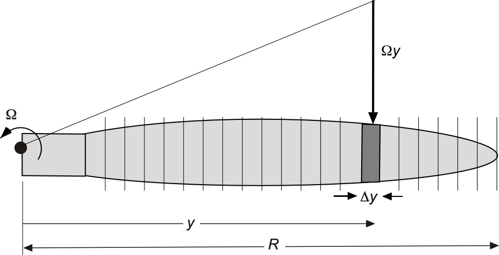
Numerical Implementation
The propeller blade can be discretized into  segments, as shown in the figure below. To give any reasonable definition of the spanwise aerodynamic loads, should be between 30 and 100. Each segment is then small enough to assume constant flow properties. Let
  denote the spanwise position of the
  -th segment, where
  , and let
  be the spanwise width of each segment.
For each segment, the resultant local velocity,  , is computed using
(72) 
and so the inflow angle is
(73) 
The local angle of attack  is then obtained using
(74) 
The local lift coefficient,  , is
, is
(75) 
If the drag coefficient  is known or assumed, e.g.,
  , it can be used directly; otherwise, the normal process is to interpolate from airfoil data tables (i.e., a table look-up approach) based on the local helical Mach number
  . Reynolds number effects can also be included if such data are available.
Computing the lift force,  , and the drag force,
  , on each segment gives
(76) 
Finally, the thrust and power contributions from all segments are then summed up using
(77) 
which, for simplicity of illustration here, uses the trapezoidal rule of integration.
MATLAB code to implement the blade element theory analysis of a propeller. Including the inflow velocity is left as an exercise for the reader.
Show code/hide code.
% Constants and input parameters
rho = 1.225; % Air density (kg/m^3)
Omega = 200; % Rotational speed (rad/s)
V_inf = 50; % Free-stream velocity (m/s)
N_b = 3; % Number of blades
R = 1.5; % Propeller radius (m)
N = 100; % Number of segments
c = 0.1; % Chord length (m)
C_l_alpha = 5.7; % Lift-curve slope
C_d = 0.01; % Profile drag coefficient
% Discretize the blade span
y = linspace(0, R, N);
dy = y(2) – y(1);
% Initialize variables
J = V_inf / (Omega * R); % Advance ratio
beta_range = deg2rad(10:1:30); % Range of blade pitch angles in radians
C_T = zeros(size(beta_range));
C_P = zeros(size(beta_range));
for k = 1:length(beta_range)
beta = beta_range(k);
% Initialize variables for each pitch angle
V = sqrt((Omega * y).^2 + V_inf^2);
phi = atan(Omega * y / V_inf);
alpha = beta – phi;
% Lift coefficient
C_l = C_l_alpha * alpha;
% Calculate lift and drag forces on each segment
dL = 0.5 * rho * V.^2 * c .* C_l * dy;
dD = 0.5 * rho * V.^2 * c * C_d * dy;
% Thrust and Power calculation
T = N_b * sum(dL .* cos(phi));
P = Omega * N_b * sum((dL .* sin(phi) + dD .* y) * dy);
% Non-dimensional coefficients
C_T(k) = T / (rho * (Omega^2) * (R^4));
C_P(k) = P / (rho * (Omega^3) * (R^5));
end
% Plot the results
figure;
plot(J, C_T, ‘-o’);
xlabel(‘Advance Ratio, J’);
ylabel(‘Thrust Coefficient, C_T’);
title(‘Thrust Coefficient vs. Advance Ratio’);
figure;
plot(J, C_P, ‘-o’);
xlabel(‘Advance Ratio, J’);
ylabel(‘Power Coefficient, C_P’);
title(‘Power Coefficient vs. Advance Ratio’);
% Output results
fprintf(‘Advance Ratio (J): %.2f\n’, J);
fprintf(‘Thrust Coefficients (C_T):\n’);
disp(C_T);
fprintf(‘Power Coefficients (C_P):\n’);
disp(C_P);
Propeller Performance Charts
Propeller performance curves are presented in terms of the thrust coefficient , power coefficient  , and propulsive efficiency , respectively, analogous to how airfoil and wing aerodynamic coefficients are used.[11] All propellers have their characteristics quantified in this manner, and there is a separate set of curves for each reference blade pitch angle. By convention, the reference pitch angle
  is not the angle of attack of the blade sections of the propeller but the reference pitch at the 75% blade span (i.e., at
  ), which is a geometric quantity and can be measured.
Helical Pitch and Slip
Often, the pitch of a propeller is measured in units of length rather than an angle. This refers to the geometric helical pitch traced by the reference blade section during one revolution, similar to a screw thread. Hence, the old name of a propeller is called an airscrew. As illustrated in the figure below, the helical pitch is the distance the propeller advances along its axis in one complete revolution, accounting for viscous effects. If the propeller were moving through a perfectly rigid medium (like a screw in a solid material), it would advance precisely the distance of its geometric pitch per revolution, as shown in the figure below. However, the propeller actually covers a shorter distance because the air deforms under its action, tracing out a helix with a lower pitch.
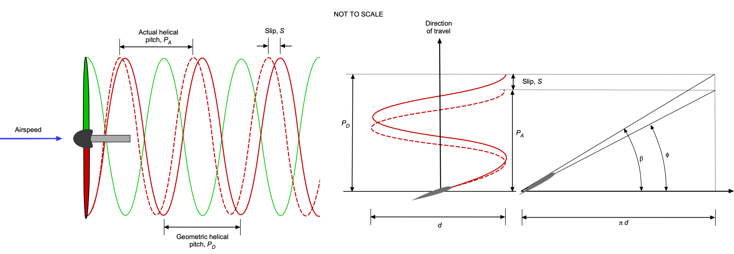
The helix angle,  , describes the inclination of the path traced by a point on the propeller blade relative to the plane of rotation. A point on the propeller blade at radius moves in a circular path with a circumferential distance per revolution given by
(78) 
Simultaneously, the propeller advances axially by  , which is given by
(79) 
where is the airspeed and is the rotational speed in revolutions per second. The helix angle is given by
(80) 
Substituting terms gives
(81) 
For a reference span station, say  , which is the conventional reference location for catalog data, the helix angle becomes
(82) 
where  is the propeller’s diameter.
A concept sometimes used to describe a propeller’s efficiency is slip, which quantifies the difference between the geometric pitch (theoretical advance per revolution) and the actual advance through the air. The propeller slip ratio,  , is defined as
(83) 
where  is the geometric pitch, i.e., the distance the propeller would ideally move forward in one revolution, and is the actual advance, i.e., the distance the propeller actually progresses through the air per revolution.
A high slip ratio indicates that the propeller is inefficient in converting rotational motion into forward thrust, whereas a low slip ratio (near zero) indicates more efficient operation. Ideally, the actual advance per revolution would equal the geometric pitch, but in practice, some slip is inevitable because of wake deformations that occur under the action of the propeller. While the slip ratio is sometimes used as an indicator of propeller performance, it has limited quantitative aerodynamic significance and should not be confused with propulsive efficiency.
Propeller Dimensions
Propeller dimensions are typically given in inches because of historical conventions in U.S. aviation, where USC units remain the industry standard for aircraft manufacturing and maintenance. This ensures consistency with aircraft manuals, FAA regulations, and existing designs, making it easier for pilots, mechanics, and manufacturers to communicate and compare specifications. Diameter and pitch are expressed in inches. For example, the Sensenich 69CK propeller has a 69-inch diameter and is available with helical pitch values ranging from 42 to 58 inches, offering options such as 69 x 42, 69 x 44, and so on. While metric conversions are used internationally, general aviation favors inches for compatibility and ease of use.
Advance Ratio
The propeller advance ratio, , is a fundamental aerodynamic parameter that helps determine a propeller’s efficiency and thrust production under different operating conditions. It connects forward motion, rotational speed, and propeller design, serving as a crucial non-dimensional parameter in propeller and rotor analysis. The advance ratio, , is defined as
(84) 
where is the airspeed (in units of m/s or ft/s), is the rotational speed of the propeller (revolutions per second, fps), and = diameter of the propeller (in units of m or ft). Physically, the advance ratio can be interpreted as the distance traveled by the propeller per revolution in terms of diameters, i.e., a non-dimensional distance or advance.
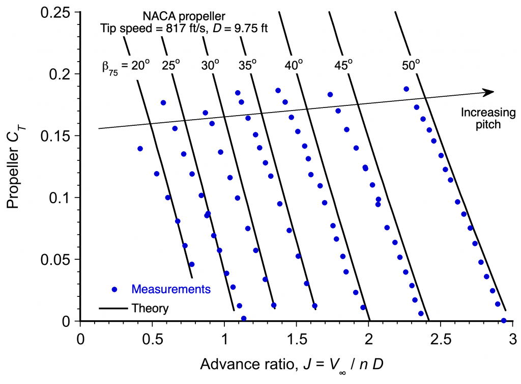
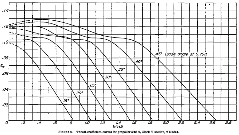
Thrust Coefficient
Recall that the thrust coefficient for a propeller is defined as
(85)
where is the thrust generated by the propeller, is the propeller’s diameter, and is the number of revolutions of the propeller per second. If the rotational angular velocity of the propeller is , then . Normally, the results for and other propeller characteristics are plotted as a function of the advance ratio, .
Representative versus results for a propeller are shown in the figure below, with a separate curve for each reference blade pitch. Notice that the results from the blade element method discussed previously (i.e., the “theory”) agree well with the measurements.
 , as a function of advance ratio, .
Power Coefficient
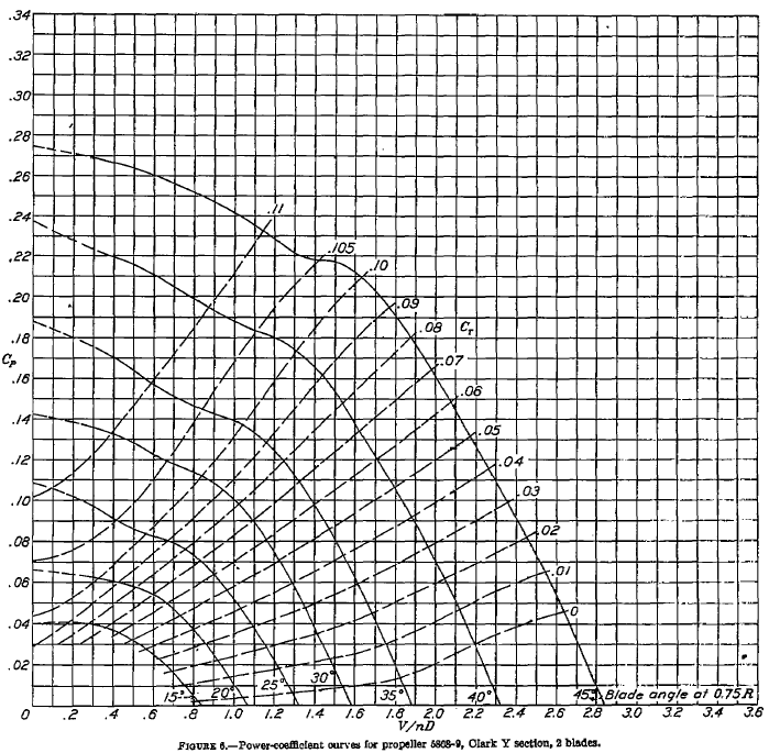
Recall that the corresponding power coefficient for the propeller is defined as
(86) 
where would be the brake power, i.e., the power delivered to the propeller through the driving shaft. Normally, the torque, , would be measured, so then =  . The corresponding versus results for a propeller are shown in the figure below. Again, notice that the theory is in good agreement with the measurements.
 , as a function of advance ratio, .
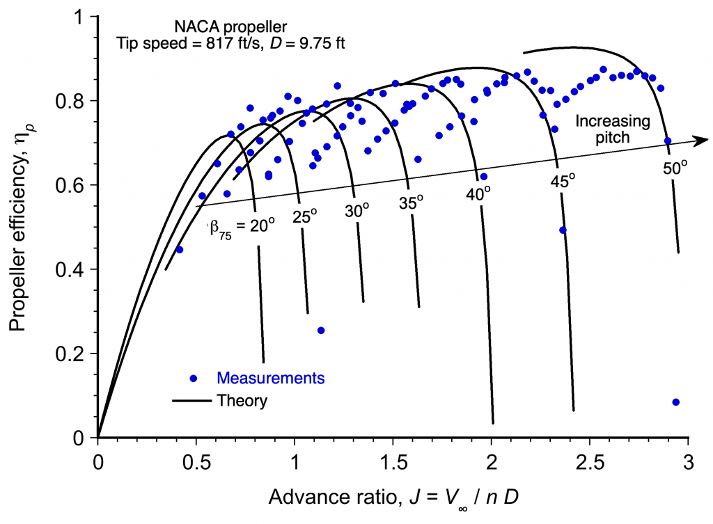
Propulsive Efficiency
Propeller efficiency measures how effectively the propeller converts available power into useful thrust. It is the ratio of useful power output (thrust power) to the total power input, i.e., engine power at the shaft or “brake” power. Propellers are typically designed for optimal performance at specific operating points. The propulsive efficiency of a propeller is defined as
(87) 
which is just a non-dimensional statement that the propeller’s efficiency is the ratio of the useful power to the input power. Notice that the symbols or are used to denote propeller efficiency, with being preferred in most contexts to avoid confusion with the propulsion system’s overall efficiency.
Using the previous definitions of and then
(88) 
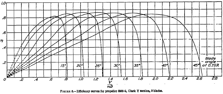
The corresponding representative versus results for a propeller are shown in the figure below, again with one curve for each reference pitch angle.
 , as a function of advance ratio, .
Notice that for a given propeller operated with any given blade pitch and rotational speed , its propulsive efficiency increases with increasing forward airspeed to reach a maximum and then diminishes rapidly. Consequently, a propeller of a given (fixed) blade pitch cannot operate with high propulsive efficiency over a wide range of values of (or airspeed for a given rotational speed).
This latter outcome occurs because propeller blades are wings (rotating wings). All wings can only operate aerodynamically over relatively small ranges of the angle of attack, i.e., local blade section angles of attack between 2 and 14 degrees, depending on the local Mach number and Reynolds number. The local sectional angles of attack on the propeller depend not only on the rotational speed of the propeller and airspeed or advance ratio but also on how the propeller is twisted along its span. So, as airspeed changes, (propeller speed in terms of revolutions per second) is assumed constant. Then, the blade pitch must be increased to progressively maintain the angle of attack on the propeller. By gradually increasing the blade pitch, the best efficiency can be obtained over a much wider range of airspeeds, which is precisely the purpose of a continuously variable pitch or “constant speed” propeller.
Reference Blade Pitch
The reference geometric blade pitch angle of a propeller, often denoted , is measured at the section located at the 3/4 radius from the rotational axis, i.e., at  . The pitch angle is taken between the local chord line of that section and the plane of rotation. It should be noted that it is a purely geometric quantity and does not represent the aerodynamic angle of attack. At that station, a material point on the blade traces a helix whose geometric helical pitch is given by
(89) 
Given a reported helical pitch value at 3/4 radius, the corresponding geometric pitch angle is
(90) 
The significance of the 3/4-radius station lies in its use of blade-element theory. The power-weighted reference station  is the radiuswise location at which an untwisted blade of constant angle
  absorbs the same power as a hyperbolically twisted blade with
  . Recall that the sectional velocity combines the rotational and axial components, i.e.,
(91) 
where
(92) 
Neglecting induced inflow corresponds to  , so that
  . The elemental torque is then
(93) 
with
(94) 
For small inflow angles,  and
and  . Under an equal-thrust comparison, the induced torque satisfies
  and cancels, so the profile torque provides the radiuswise weighting
  .
.
For a blade with uniform chord  with no root cutout, the power-weighted station is
(95) 
Substituting  gives the numerator as
(96) ![\begin{equation*} \int_{0}^{1} U^2\,r\,dr=(\Omega R)^2\left[\int_{0}^{1} r^3\,dr + a^2\int_{0}^{1} r\,dr\right] =(\Omega R)^2\left(\frac{1}{4}+\frac{a^2}{2}\right) \end{equation*}](https://eaglepubs.erau.edu/app/uploads/quicklatex/quicklatex.com-93d68861fc01f8a9addbfe8ca4cdeea7_l3.svg "Rendered by QuickLaTeX.com")
and the denominator as
(97) ![\begin{equation*} \int_{0}^{1} U^2\,dr=(\Omega R)^2\left[\int_{0}^{1} r^2\,dr + a^2\int_{0}^{1} dr\right] =(\Omega R)^2\left(\frac{1}{3}+a^2\right) \end{equation*}](https://eaglepubs.erau.edu/app/uploads/quicklatex/quicklatex.com-d2e92865a1593e7cf84291e5e2906421_l3.svg "Rendered by QuickLaTeX.com")
Forming the ratio and cancelling  gives
gives
(98) 
In the small-inflow limit  , then
(99) 
which places the reference station at three-quarters radius. Increasing airspeed (larger  ) moves the station slightly further inboard according to the closed-form expression above, but it remains close to
  , which is why this location is used as a fixed reference. Once is determined, the geometric helical pitch of the propeller can be reported as
(100) 
Further Discussion of Propeller Performance
With this understanding of the flow at the blade section and the creation of thrust from the propeller, the various curves of , , and , as shown previously, can now be explained in greater detail. At low values of , the corresponding angles of attack of the blade sections are relatively high. So, the blade sections produce relatively high lift but are close to the point of stall. The propeller still produces thrust but requires high power and is inefficient. As airspeed and increase, the blade sections operate at lower angles of attack and closer to their best section lift-to-drag ratios. As a result, thrust is maintained while drag on the blades decreases, leading to a significant increase in propulsive efficiency.
The lowest angles of attack will produce little lift on the blades or thrust on the propeller. However, there is a range of airspeeds (assuming blade pitch does not change) for which good propulsive efficiency is obtained. Therefore, the best aerodynamic efficiencies will only be obtained when all or most blade sections operate at or near the angles of attack that yield their best lift-to-drag ratio, which is typically between 2 and 8 degrees, depending on the incident Mach number.
There is eventually a point at higher airspeeds (or high ) where the blade sections encounter diminished angles of attack and higher helical Mach numbers, simultaneously decreasing thrust and efficiency unless the blade pitch increases further. Eventually, the blade pitch cannot be mechanically increased to improve efficiency, so efficiency decreases.
Propulsive Efficiency
The results also explain the differences in propulsive efficiency of fixed-pitch versus constant-speed propellers, as shown in the figure below. Notice that if the propeller pitch is fixed, its propulsive efficiency increases slowly with airspeed, reaches a maximum, and then decreases rapidly. The relatively low efficiency of a fixed-pitch propeller at low airspeeds results in poor takeoff and climb performance for the aircraft. Further increases in airspeed beyond the airspeed for peak efficiency will cause propeller efficiency to decrease precipitously. This behavior reduces the power delivered to the airstream as useful work, effectively setting an upper barrier to the airspeed achievable by the airplane.
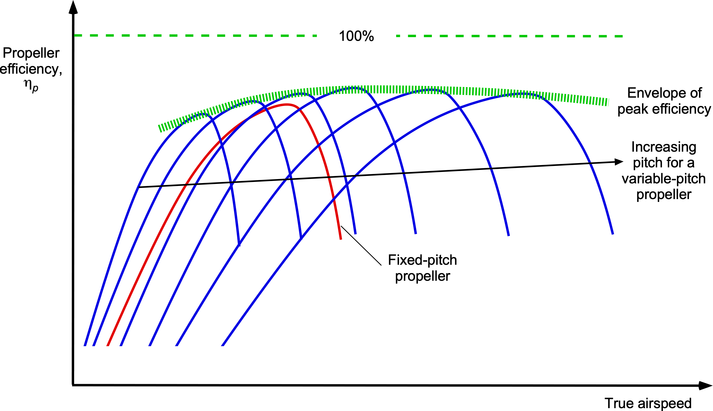
The preceding situation is very different for a variable-pitch or constant-speed propeller, which can be set to a fine pitch for takeoff. This provides good propulsive efficiency and low airspeed, resulting in markedly better takeoff and climb performance for the airplane. As airspeed increases, the blade pitch can be adjusted to maintain a constant rpm schedule, allowing the propeller efficiency to closely track the peak efficiency envelope. This reason is why airplanes with constant-speed propellers have much better overall flight performance and can cruise at much higher airspeeds, as shown in the figure below. A constant-speed propeller also maintains a steady load on the engine, which is essential for long engine life.
Worked Example #1 – Calculating propeller performance
Refer to the propeller charts below, which are a standard performance presentation for all propellers. Assume that an actual propeller has a diameter of 7 ft and is a constant-speed propeller with a rotational speed of 2,000 rpm. The propeller operates at an equivalent density altitude of 8,000 ft ISA.
 For each blade pitch angle measured at 75% radius and at the point of maximum propulsive efficiency in each case, estimate the following:
(a) What are the advance ratio values and corresponding airspeed values?
(b) What are the propeller thrust coefficient values and the propeller’s corresponding thrust?
(c) What are the values of the propeller power coefficient and the corresponding shaft torque and power required to rotate the propeller?
Show solution/hide solution.
(a) At the peak efficiency, the values of the advance ratio can be read off the first chart. We can easily do this to two decimal places; the chart can be digitized for better accuracy. We are also given information about the specific propeller, which is relatively small and would likely be for a general aviation aircraft, so in each case, we can calculate the corresponding airspeed for a given value of , i.e.,
![\[ J = \frac{V_{\infty} }{n \, d} =\frac{V_{\infty} }{(\text{\small rpm}/60) \, d} \]](https://eaglepubs.erau.edu/app/uploads/quicklatex/quicklatex.com-bee8d97dbd941f3bd1428463737b28af_l3.svg "Rendered by QuickLaTeX.com")
so
![\[ V_{\infty} = J \, (\text{\small rpm}/60) \, d = J (2,000/60) \times 7.0 = 233.34 \, J~\mbox{ft/s} \]](https://eaglepubs.erau.edu/app/uploads/quicklatex/quicklatex.com-268ce4dbe9e1753370d00cb95faf851a_l3.svg "Rendered by QuickLaTeX.com")
It is best to use a table to show the results, i.e.,
Blade pitch ( ) ) |
|
|
(ft/s) |
| 15 | 0.82 | 0.65 | 151.7 |
| 20 | 0.85 | 0.82 | 191.3 |
| 25 | 0.87 | 1.04 | 242.7 |
| 30 | 0.87 | 1.25 | 292.7 |
| 35 | 0.86 | 1.45 | 338.3 |
| 40 | 0.86 | 1.70 | 398.7 |
| 45 | 0.84 | 1.95 | 455.0 |
(b) The propeller thrust coefficient can be read off the second chart for each value of the advance ratio, as was identified in the previous part. The thrust coefficient for a propeller is defined as
![\[ C_T = \frac{T}{\varrho_{\infty} \, n^2 \, d^4} \]](https://eaglepubs.erau.edu/app/uploads/quicklatex/quicklatex.com-12918c2b351ae6f7a4aaf44f9af4fb7d_l3.svg "Rendered by QuickLaTeX.com")
so the corresponding thrust (in units of force) from the propeller is
![\[ T = \varrho_{\infty} n^2 \, d^4 \, C_T \]](https://eaglepubs.erau.edu/app/uploads/quicklatex/quicklatex.com-bbbf224490b13172c49ba78422812383_l3.svg "Rendered by QuickLaTeX.com")
We are told that the propeller operates at an equivalent density altitude of 8,000 ft ISA. According to the ISA equations, the density at this altitude is 0.001869 slugs/ft . Inserting the information gives
![\[ T = \varrho_{\infty} \, n^2 \, d^4 \, C_T = 0.001869 \times \left( \frac{2000}{60} \right)^2 \times 7.0^4 \, C_T = 4986.08 \, C_T \]](https://eaglepubs.erau.edu/app/uploads/quicklatex/quicklatex.com-c33693eaf6cb5819495fd81457754db0_l3.svg "Rendered by QuickLaTeX.com")
Again, it is best to use a table to show the results, i.e.,
| Blade pitch () |
|
|
|
| 15 | 0.65 | 0.025 | 124.7 |
| 20 | 0.82 | 0.038 | 189.5 |
| 25 | 1.04 | 0.040 | 199.4 |
| 30 | 1.25 | 0.047 | 234.4 |
| 35 | 1.45 | 0.052 | 259.3 |
| 40 | 1.70 | 0.060 | 299.2 |
| 45 | 1.95 | 0.072 | 359.0 |
(c) The propeller power coefficient can be read off the third chart for each value of the advance ratio identified in the previous part. The power coefficient for a propeller is defined as
![\[ C_P = \frac{P}{\varrho_{\infty} \, n^3 \, d^5} \]](https://eaglepubs.erau.edu/app/uploads/quicklatex/quicklatex.com-616df2c161ec608d4a5e92277931e562_l3.svg "Rendered by QuickLaTeX.com")
so the corresponding power needed to drive the propeller is
![\[ P = \varrho_{\infty} \, n^3 \, d^5 \, C_P \]](https://eaglepubs.erau.edu/app/uploads/quicklatex/quicklatex.com-16eeea4c16aa556fa5590d8dd2a44458_l3.svg "Rendered by QuickLaTeX.com")
Inserting the known information gives
![\[ P = \varrho_{\infty} \, n^3 \, d^5 \, C_P = 0.001869 \times \left( \frac{2000}{60} \right)^3 \times 7.0^5 \, C_P = 2115.31 \, C_P \]](https://eaglepubs.erau.edu/app/uploads/quicklatex/quicklatex.com-71390e78a836d790120b5a6d75370bd2_l3.svg "Rendered by QuickLaTeX.com")
where the conversion to horsepower (hp) is obtained by dividing the result in ft-lb s by 550. Again, it is best to use a table to show the results, i.e.,
| Blade pitch () |
|
|
(hp) |
| 15 | 0.65 | 0.022 | 46.5 |
| 20 | 0.82 | 0.035 | 74.0 |
| 25 | 1.04 | 0.048 | 101.3 |
| 30 | 1.25 | 0.065 | 137.5 |
| 35 | 1.45 | 0.09 | 190.3 |
| 40 | 1.70 | 0.12 | 253.8 |
| 45 | 1.95 | 0.17 | 359.7 |
Helical Tip Mach Number
As airspeed and the values of increase, a concern is that the tip speed of the propeller can approach supersonic conditions. If this condition occurs, the propeller loses propulsive efficiency and produces more noise. This reduction in efficiency means that more power is required to make the same amount of thrust, which can adversely affect fuel consumption and overall flight performance. Supersonic airflow generates shock waves, resulting in a dramatic increase in propeller noise. A propeller’s noise is a significant concern in aviation, impacting passenger comfort, community acceptance, and regulatory compliance.
Let  be the helical tip velocity based on the vector sum of the rotational and airspeed components at the blade elements. Therefore, the rotational tip speed of a propeller characterized by radius or diameter (= 2) is
(101) 
and so the helical tip speed of the propeller is
(102) 
where is the forward airspeed. Therefore, the helical Mach number  will be
(103) 
where is the speed of sound at the atmospheric conditions at which the propeller operates.
The measurements shown in the figure below, for a high-speed NACA propeller with thin blades, eventually reach supersonic helical-tip Mach numbers. In this case, the measurements were taken at a constant blade pitch to examine variations in rotational speed. Notice that rapid losses in propulsive efficiency (from a peak of about 0.95) are produced at higher airspeeds if the rotational tip speeds are kept at high values. Compressibility losses increase when the helical tip Mach number reaches about 0.8. While every propeller will be different, exceeding some limiting critical tip Mach number at the blade tip, which may be around 0.7 for a standard blade and 0.8 for a thin airfoil section and swept leading edge at the tip, can be expected to decrease propulsive efficiency, increase noise, or, more usually, both.
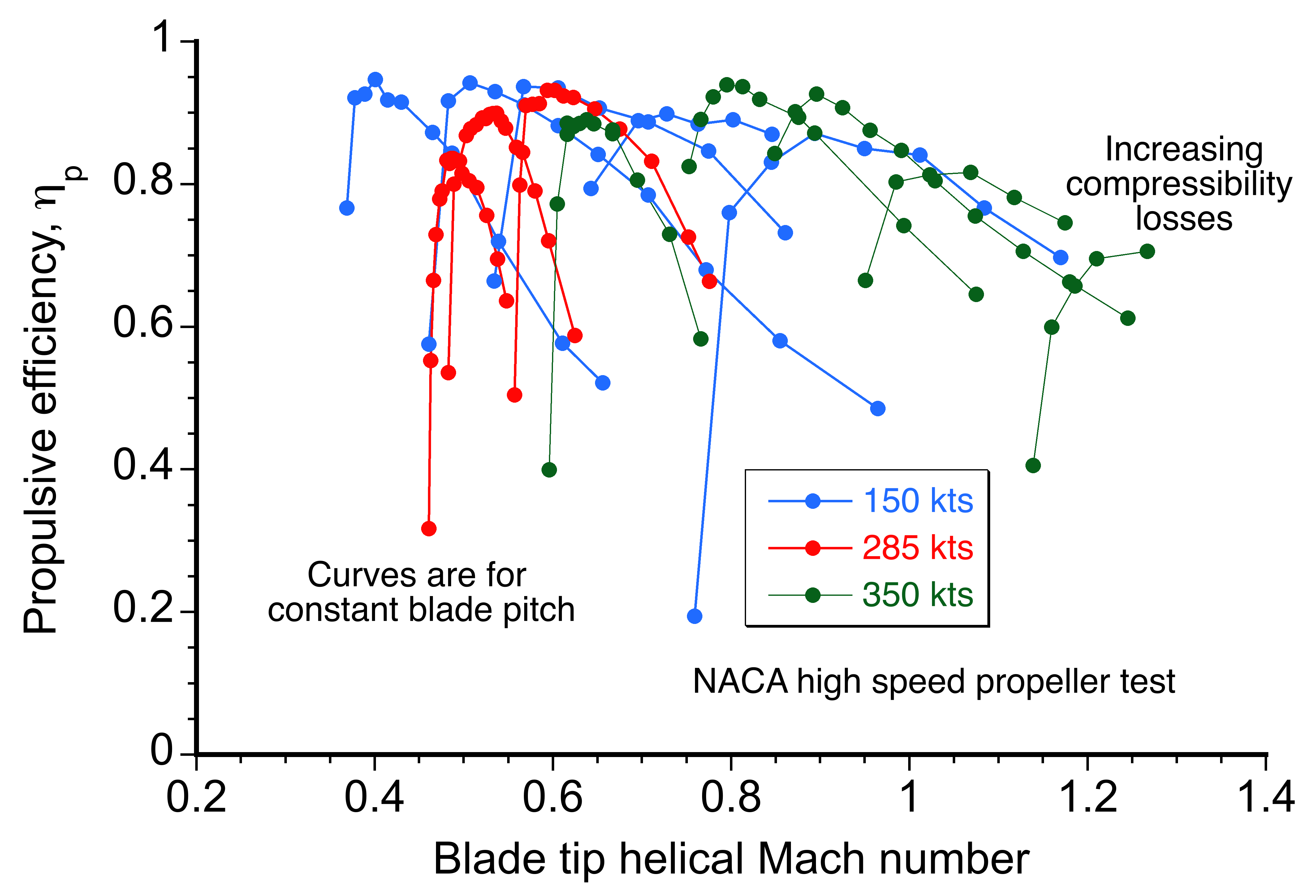
Propeller Noise
Propeller noise is a significant contributor to the acoustic signature of propeller-driven aircraft, particularly during takeoff, climb, and high-speed cruise flight. It originates from unsteady aerodynamic forces acting on the blades and from compressibility effects at high tip speeds. Unlike rotorcraft, conventional single-rotor airplane propellers do not experience blade-wake or blade-vortex interaction noise. Instead, the dominant sources are thickness noise, loading noise, compressibility noise, and shock waves originating at the blade tips.
Thickness noise arises from the periodic displacement of air by the rotating blades. This type of noise radiates at the blade-passing frequency and integer multiples of its harmonics. Aerodynamic forces generate loading noise, primarily from blade lift. It is most intense during high-thrust phases such as takeoff and climb. Both sources contribute to the prominent tonal peaks in the noise spectrum.
As the tip Mach number approaches or exceeds 0.85, compressibility effects become significant, and localized shock waves may form near the blade tips. This results in a significant increase in noise amplitude, harshness, and high-frequency content. The noise becomes impulsive in character and highly directional. The schlieren image below illustrates this phenomenon for  , showing spiraling acoustic Mach waves forming at the blade tips. These waves compress and intertwine into a rotating analog of a Mach cone produced by an airplane flying near the speed of sound, similar in character to a forming sonic boom. Also visible are the tip vortex and the turbulent blade wake, which contribute additional high-frequency acoustic content.
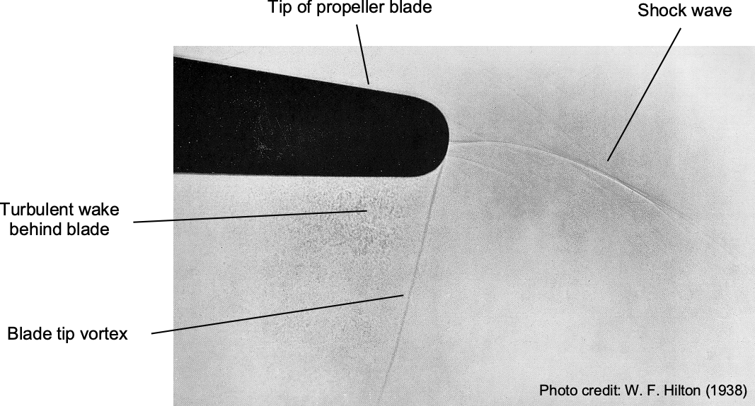
The dominant source of propeller noise in airplane applications is loading or monopole noise, generated by unsteady aerodynamic forces acting on the rotating blades. These effects can be modeled as a dipole source, and the far-field acoustic power radiated by such a source increases rapidly with blade tip speed. From classical aeroacoustic theory, the acoustic power radiated by a rotating blade system can be approximated as
(104) 
where  is the radiated acoustic power,
  is the freestream air density,
  is the aerodynamic force on the blade, is the angular velocity of the propeller, is the blade radius, and
  is the freestream speed of sound. The aerodynamic force scales with dynamic pressure, giving
  . Therefore, substituting into the expression for leads to
(105) 
Furthermore, using the rotational tip Mach number  gives
gives
(106) 
Because the sound pressure level (SPL) scales logarithmically with acoustic power, then
(107) 
and finally leading to the propeller noise scaling law with tip Mach number, i.e., the sound pressure level is
(108) 
In practice, empirical measurements often yield a slightly lower exponent due to effects other than ideal conditions, such as non-uniform inflow, installation interference, and atmospheric absorption. A more commonly used representation is
(109) 
The dominant frequency of propeller noise corresponds to the blade-passing frequency, defined as
(110) 
where is the number of blades and  is the shaft rotational frequency. Tonal components, associated with thickness and loading noise, tend to dominate the acoustic spectrum and are most intense at the blade-passing frequency and its harmonics. Broadband noise arises from turbulence ingestion, unsteady blade loading, and distorted inflow conditions. The radiation pattern is highly directional, with tonal noise being strongest in the plane of rotation, while loading noise is primarily radiated in a direction parallel to the thrust axis.
Several strategies exist to reduce propeller noise. Limiting tip speed is essential to avoid shock-induced impulsive noise, which can be managed by selecting a larger diameter or reducing the rotational speed. Increasing the number of blades reduces the per-blade loading and shifts tonal energy to higher, more attenuated frequencies. Careful blade design, including sweep, twist, and taper, helps minimize unsteady aerodynamic forces and delay the onset of compressibility effects. Finally, installation effects are critical; distorted inflow caused by fuselage or wing boundary layers can exacerbate noise, especially in pusher configurations. Tractor propeller arrangements, with cleaner inflow conditions, typically offer lower noise levels for a given thrust.
Example #2 – Calculating a propeller’s helical tip Mach number
Refer back to Worked Example #1. What are the propeller’s helical tip speed values and helical Mach number? Comment on your results. Note: The helical tip speed is the vector sum of the rotational speed at the tip of the propeller and the freestream (airspeed).
Show solution/hide solution.
Let be the helical tip velocity based on the vector sum of the rotational and airspeed components. The rotational tip speed of a propeller of diameter is
![\[ V_{\rm tip} = \Omega \left( \frac{d}{2} \right) \]](https://eaglepubs.erau.edu/app/uploads/quicklatex/quicklatex.com-cd06b55eefcd43262a470514ae93fe71_l3.svg "Rendered by QuickLaTeX.com")
where  and so the helical tip speed of the propeller is
![\[ V_{\rm hel} = \sqrt{ V_{\rm tip}^2 + V_{\infty}^2} \]](https://eaglepubs.erau.edu/app/uploads/quicklatex/quicklatex.com-b55bfac40b3fa5db14899e9f160d232c_l3.svg "Rendered by QuickLaTeX.com")
where  is the forward airspeed. The helical Mach number will be
![\[ M_{\rm hel} = \frac{V_{\rm hel} }{a} \]](https://eaglepubs.erau.edu/app/uploads/quicklatex/quicklatex.com-84b11982f69400ea55a6bdd5b2e4a900_l3.svg "Rendered by QuickLaTeX.com")
where  is the local speed of sound at the conditions at which the propeller operates. At 8,000 ft ISA density altitude,
  1085.3 ft/s.As a final table to show the results, the helical tip speed and Mach number are:
| Blade pitch () |
|
(ft/s) |
(ft/s) |
|
| 15 | 0.65 | 151.7 | 748.6 | 0.69 |
| 20 | 0.82 | 191.3 | 757.6 | 0.70 |
| 25 | 1.04 | 242.7 | 772.2 | 0.71 |
| 30 | 1.25 | 292.7 | 788.9 | 0.73 |
| 35 | 1.45 | 338.3 | 807.3 | 0.74 |
| 40 | 1.70 | 398.7 | 833.5 | 0.77 |
| 45 | 1.95 | 455.0 | 862.8 | 0.79 |
We notice that for an airspeed above 400 ft/s, the propeller blade tips would likely begin to operate near or just beyond the critical Mach number (i.e., the onset of transonic flow), which for the thin tips of propeller blades is about 0.8. Under these conditions, the propeller will likely lose propulsive efficiency.
Propeller Selection Process
Propeller selection must match the aircraft’s mission, performance goals, and propulsion system. Key factors include thrust requirements across flight phases, powerplant type (piston, turboprop, or electric), cruise efficiency, and installation constraints. The propeller diameter has a significant impact on thrust, power consumption, and efficiency. Larger diameters enhance low-speed performance but may be limited by ground clearance, airframe geometry, or high tip speeds. At higher rpm, blade tips must remain subsonic to avoid compressibility losses and the rapid increase in noise associated with the tip Mach number.
The blade count affects the amount of thrust a propeller can produce for a given diameter. More blades allow the disk to absorb greater power, which is helpful for high-power engines or when the diameter is constrained by ground clearance or airframe layout. However, additional blades add weight, drag, and mechanical complexity, especially in variable-pitch systems. Blade geometry must also be optimized spanwise to maintain efficiency across varying inflow conditions. Key factors include the airfoil section, chord distribution, and twist, which typically follow a hyperbolic pattern from the root to the tip.
Variable-pitch or constant-speed propellers maintain propulsive efficiency by adjusting blade angles in flight and are standard on high-performance piston and turboprop aircraft. Material selection also matters. Wood is lightweight and inexpensive, but it is limited to low-power use under 200 shp (149.4 kW). In contrast, aluminum is at least three times stronger but approximately six times heavier by volume. Composite blades combine low weight with high strength, allowing for thinner, more efficient shapes in high-speed turboprop applications.
The propeller must also match the engine’s power and torque characteristics. Piston engines operate efficiently at lower rpm (less than 3,000) and can often drive propellers directly. Turboshaft engines typically require a reduction gearbox, although free-turbine designs are also common and efficient.[12] Electric motors, with high torque at low rpm, can also drive large, slow-turning propellers directly, in the range 4,000 to 8,000 rpm. Additional concerns for propeller integration include vibration, noise, and inflow distortion, particularly in pusher configurations affected by an upstream wake. A successful design will strike a balance among these factors to deliver efficient, reliable, and quiet propulsion that suits the aircraft and its mission.
Steps for Propeller Selection
The following are the specific steps that are involved in the selection of a propeller:
- Define the mission profile and flight envelope. These requirements may include the maximum takeoff weight, cruise speed and altitude, climb performance, and powerplant characteristics and limitations such as available power and allowable rotational speed (rpm) range. Airframe installation constraints, such as ground clearance or nacelle position, must also be considered.
- Estimate thrust and power requirements. Use aircraft drag estimates and mission analysis to determine the required thrust during takeoff, climb, and cruise. Combine this with available shaft power from the powerplant to calculate the required propeller efficiency.
- Select a candidate propeller diameter and rotational speed. Select a diameter that provides sufficient disk area for thrust without exceeding the tip Mach number limit of approximately 0.85 at the maximum propeller rpm, thereby minimizing compressibility losses.
- Choose or design a blade geometry. For custom designs, one can use blade-element theory (BET) or similar methods to determine the optimal twist and planform (chord) distributions. For off-the-shelf options, consult the manufacturer’s data sheets and performance characteristics (e.g., curves) to determine the thrust coefficient, power coefficient, and efficiency, which will help select the propeller.
- Calculate the advance ratio and match it to the performance requirements. Use the parameter to find the operating point of the aircraft, then compare it to the propeller performance curves. One generally aims to operate the propeller near its peak efficiency at cruise, while still ensuring sufficient thrust and propulsive efficiency at lower airspeeds, such as takeoff.
- Determine whether variable pitch is required. If the flight conditions span a wide range of flight speeds or power settings, a variable-pitch propeller may be needed to maintain the propulsive efficiency. Fixed-pitch or ground-adjustable designs are simpler but can be optimized for only one flight condition.
- Evaluate structural and material choices. Consider blade loads, centrifugal forces, vibration, and the possibilities of material fatigue. Common materials include wood, aluminum, and composite, each with its own trade-offs in terms of weight, strength, durability, and cost.
- Integrate with the engine and airframe. Ensure compatibility with the engine’s torque curve and power output. It may be necessary to account for airframe-induced inflow distortion, especially in pusher configurations. Validate hub mounting, spinner clearance, and “ram” airflow to the cooling system.
- Test and refine the selection. After the preliminary design or selection, the propeller’s performance must be verified through ground runs and flight testing. Normally, aircraft manufacturers instrument the powerplant and aircraft to record enough parameters to verify or revise the prepropeller design as needed, based on flight test data.
Speed-Power Coefficient (Weick) Method
The speed-power coefficient,  , is a non-dimensional parameter introduced by Fred Weick at NACA to characterize propeller performance independently of physical dimensions, such as diameter or blade pitch. Weick originally used the coefficient to develop empirical performance maps of propeller efficiency, thereby reducing or eliminating the need for wind-tunnel or shaft-torque (i.e., dynamometer) measurements. This approach remains useful today, particularly when evaluating geometrically similar propellers or analyzing flight data from smaller propeller-driven aircraft. While the advance ratio is central to the selection and aerodynamic design of propellers, the coefficient often proves more practical for interpreting in-flight performance, particularly under less-than-ideal operating conditions. In the case of fixed-pitch propellers, which are efficient only over a small range of conditions, the value of at the intended operating conditions helps identify the most appropriate propeller. This is because it links flight speed, power, and rpm to the known or predicted performance characteristics of both the powerplant and the aircraft.
Definition and Derivation
Weick[13] noted that while the , , and coefficients help compare the thrust, torque, and power of different propellers, “they are not particularly helpful, however, in selecting or designing propellers to fit certain specific requirements for driving some form of airplane.” Furthermore, Weick noted that “the parameter  is not a fair basis upon which to compare the efficiencies of various propellers that might fit the same aircraft at the same values of and but have different diameters, , and, therefore, other values of
  .”
.”
To this end, Weick showed that a new dimensionless propeller coefficient involving , , and without may be obtained from and  using
using
(111) 
where  is the air density, is the true airspeed of the propeller through the air, is the shaft power available to the propeller, and is the propeller’s rotational speed in revolutions per second. An alternative form, which keeps the numerical values within a reasonable range, is in terms of the fifth root of the previous expression, where
(112) ![\begin{equation*} C_S = \sqrt[5]{\frac{\varrho_{\infty} \, V_{\infty}^5}{P \, n^2}} = V_{\infty} \sqrt[5]{\frac{\varrho_{\infty}}{P \, n^2}} \end{equation*}](https://eaglepubs.erau.edu/app/uploads/quicklatex/quicklatex.com-4ca3408de5a601c1bed9d80266abb9a7_l3.svg "Rendered by QuickLaTeX.com")
Notice that the numerical values of must be calculated using consistent engineering units.
It should be apparent that is called a “speed-power” coefficient because it contains the rotational and forward speeds and the power that the propeller needs to absorb.[14] The diameter and pitch selection of a propeller is based on identifying the optimal balance between efficiency and operational constraints under specific design conditions for the aircraft. The power required for flight depends on the aircraft and its operating conditions. Because a fixed-pitch propeller operates most efficiently at a single point in its performance envelope, the coefficient can help determine the best-matched propeller for the desired airspeed and power available at the propeller’s shaft.
Practical Usage and Application
The speed-power coefficient has several practical applications, including the selection of fixed-pitch propellers, in-flight performance testing, and aircraft performance analysis, particularly when complete aerodynamic data are unavailable. In many aircraft test programs, thrust is not directly measurable, but airspeed, rpm, shaft power, and air density are usually obtainable. Because the coefficient incorporates both power and air density, it naturally accounts for variations in throttle setting and density altitude, allowing test data from different flight conditions to be reduced to a more consistent and useful form.
Wind Tunnel Testing
The value of the coefficient can first be explained with reference to propeller performance measurements made in the wind tunnel. Propeller testing in the tunnel often involves using a series of geometrically similar designs, with pitch and airspeed variations applied in uniform increments. For example, the NACA tested propellers in its 20-foot wind tunnel using a system that allowed continuous pitch adjustments over an extensive range of angles and at increasing airspeeds, until the blade tips exceeded their critical Mach numbers. High helical tip Mach numbers typically set a limit on propeller operation in terms of efficiency and noise, or sometimes both. For a fixed-pitch propeller of a given blade design, the range of pitch angles that are available is typically limited to only two or three.
If performance data are available for candidate propellers, the corresponding value can also be calculated and compared with the efficiency curves. Start with the definition that
(113) 
The propulsive efficiency is given by
(114) 
Substituting the standard expressions for and into the definition of gives
(115) 
and substituting into the expression for gives
(116) 
Simplifying gives the result that
(117) 
which can be evaluated from the data comprising the standard propeller “ curves.”
An example of this type of analysis is shown in the figure below. The curves in the plot show the values of as a function of advance ratio for each blade pitch, along with the corresponding curves of propeller efficiency . The “curve of best efficiency” traces a locus of operating points where each propeller configuration operates most efficiently. By computing for a desired flight speed, shaft power, and rpm, one can find the corresponding and select a propeller diameter that places the powerplant-aircraft system near this optimal propeller curve. Alternatively, for a given propeller and value, the use of allows the power and revolutions per second available from a given powerplant to be matched to this propeller.
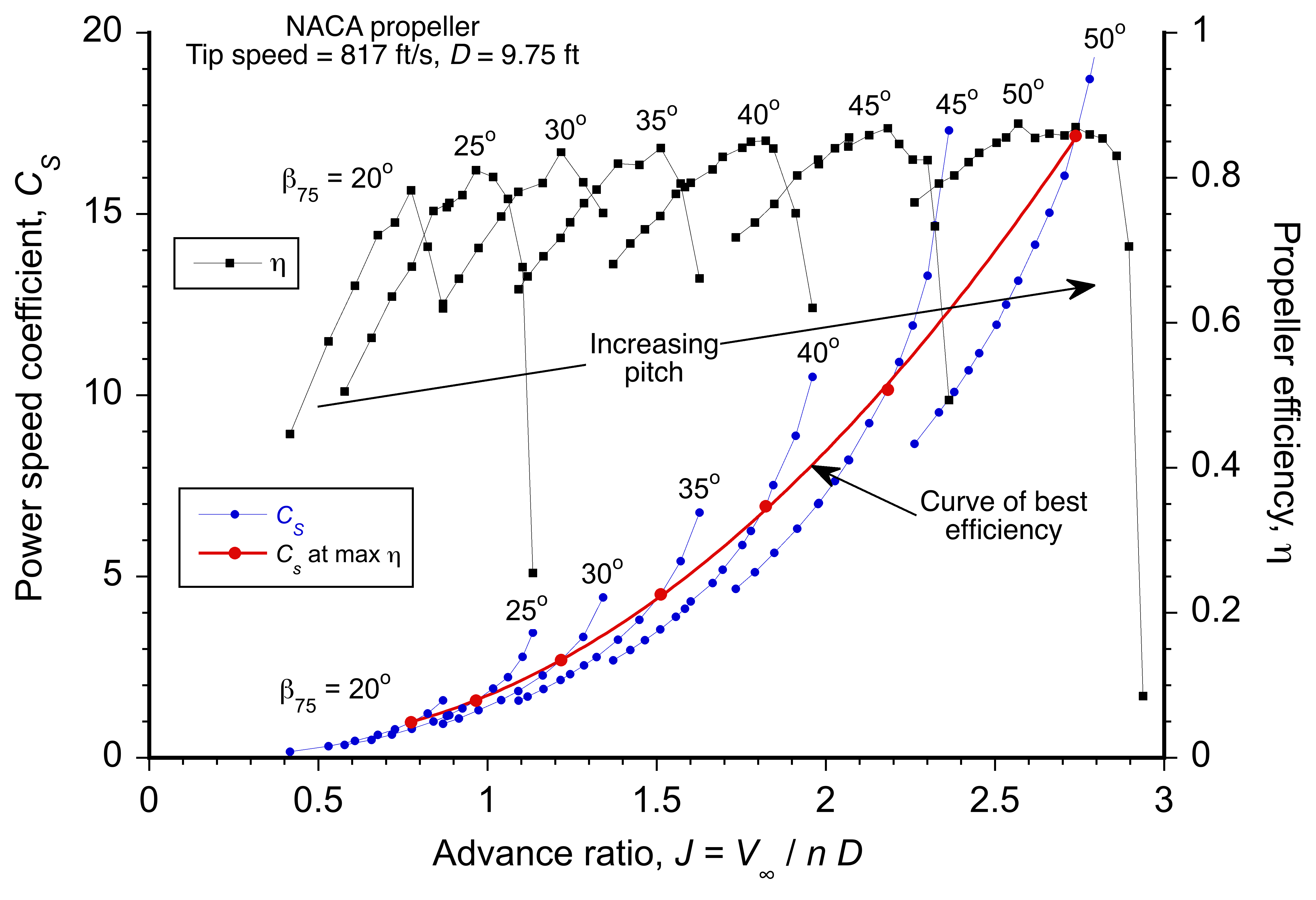 as a function of advance ratio , along with curves of propeller efficiency at various blade pitch angles.
If the desired advance ratio is known or can be determined, then the corresponding propeller diameter is computed using
(118) 
The blade pitch is then chosen so that the propeller exhibits peak efficiency near the target , with a deliberate bias toward lower values to avoid performance degradation at takeoff and climb. This trade-off is necessary because fixed-pitch propellers cannot be adjusted in flight. Alternatively, the propeller speed, , can be chosen for a given propeller diameter, i.e.,
(119) 
It should be noted that, regarding wind tunnel testing, the coefficient does not provide any additional information about propeller selection, as the diameter and pitch required to meet a given level of performance can be determined entirely from the “-curves.” What it does do, however, is verify that the selected propeller matches the power available from the powerplant at a given airspeed and density altitude, and that the corresponding values of the and coefficients are within the normal operating range of that propeller and are close to the line of best propulsive efficiency. This approach ensures that the chosen propeller utilizes the available power efficiently, neither overloading nor underloading it.
Flight Testing
In flight testing, the speed-power coefficient provides a valuable means of assessing propeller performance when the propeller “ curves” are unavailable. Its utility lies in the fact that all of the constituent terms of , i.e.,
(120) ![\begin{equation*} C_S = V_{\infty} \sqrt[5]{\frac{\varrho_{\infty}}{P \, n^2}} \end{equation*}](https://eaglepubs.erau.edu/app/uploads/quicklatex/quicklatex.com-1b6cc813a530acc54556be0e02c4340f_l3.svg "Rendered by QuickLaTeX.com")
can be obtained from basic flight instrumentation. The airspeed is measured using a Pitot-static system and corrected, if necessary, by local air density to provide the true airspeed,  . The air density is computed from measurements of ambient pressure and temperature using the equation of state, or from pressure altitude and temperature measurements and using the ISA model.
The shaft power can be estimated from powerplant data in terms of performance charts or “decks” in the form of numerical data. For example, for piston engines, the shaft power required to compute is estimated using engine performance data that correlates manifold pressure, engine rpm, pressure altitude, and outside air temperature with brake power (e.g., bhp) output. These values are measured from the aircraft’s engine instruments and, in post-flight analysis, are cross-referenced against charts or tables provided by the engine manufacturer. This indirect method, while approximate, is sufficiently accurate for trend analysis and performance comparison. For electric motors, the electrical input power, measured in volts and amps, can be measured during flight and corrected for by the motor’s electrical-to-mechanical efficiency, i.e., through a calibration.
By evaluating at a sequence of flight-test points for different values of , engineers can assess the suitability of a given propeller, evaluate off-design behavior, and ensure proper matching between the propeller and powerplant, all without needing detailed propeller “-curves.” As shown in Fig.~??, which comprises notional flight-test data, the most suitable propeller(s) for the aircraft will exhibit data points that cluster tightly or trend smoothly. This outcome suggests the propeller is a good match for the powerplant and the aircraft. If the data points exhibit significant scatter and inconsistent trends, this outcome suggests a less suitable, or even an unsuitable, propeller. Multiple flights with each propeller should be conducted to establish definitive trends.
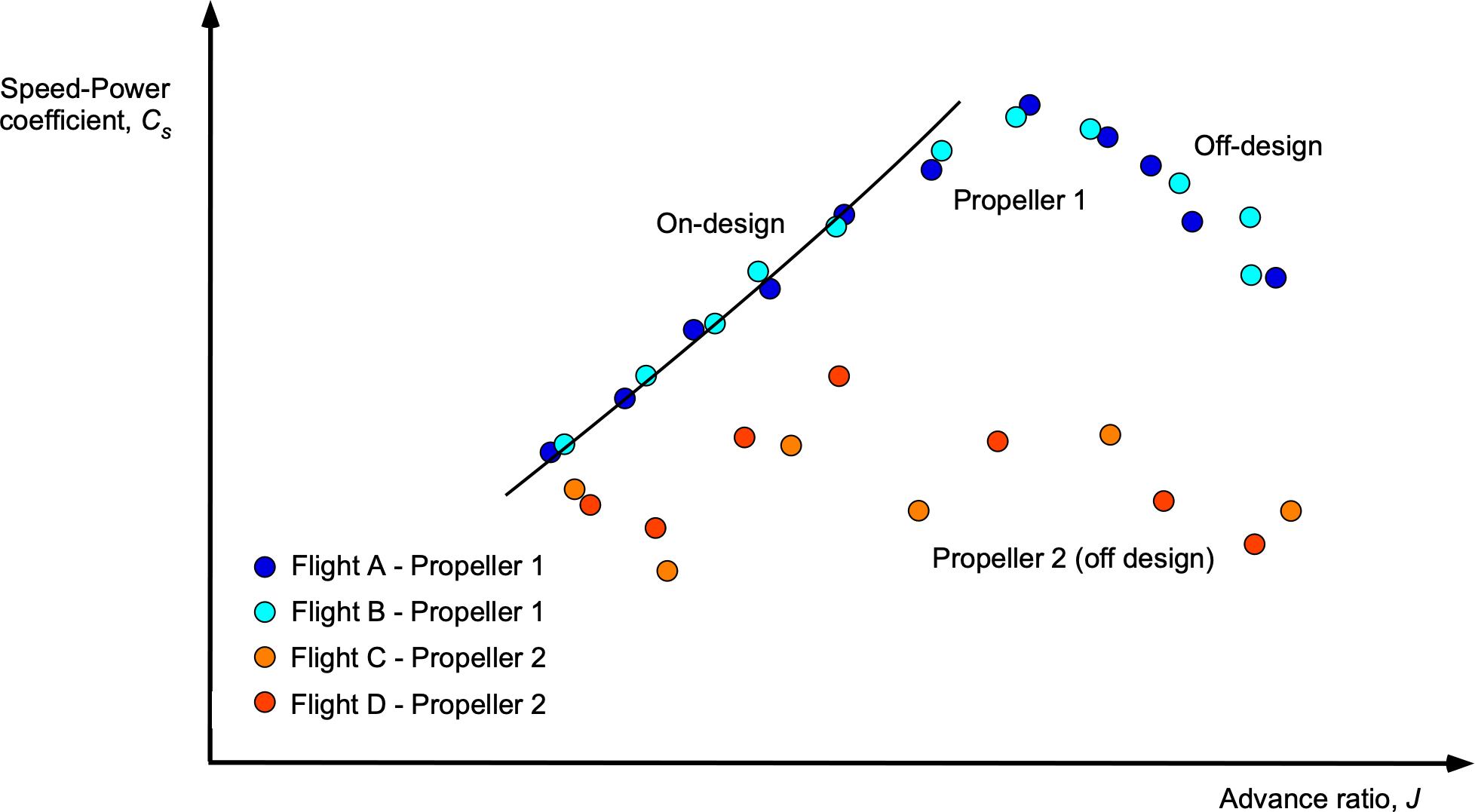 and from flight test data will bring out the most suitable propellers that match the powerplant and the aircraft.
Pusher Propellers
Tractor propellers, mounted at the front of the aircraft and operating in undisturbed freestream flow, are the most common configuration in aircraft design. However, numerous aircraft have been developed with pusher propellers, where the propeller is located aft of the fuselage or wing structure. In this arrangement, the propeller operates in the airframe’s wake, which can affect its aerodynamic performance. Today, pusher configurations are frequently employed in uncrewed aerial vehicles (UAVs) and drones, as illustrated in the photograph below.
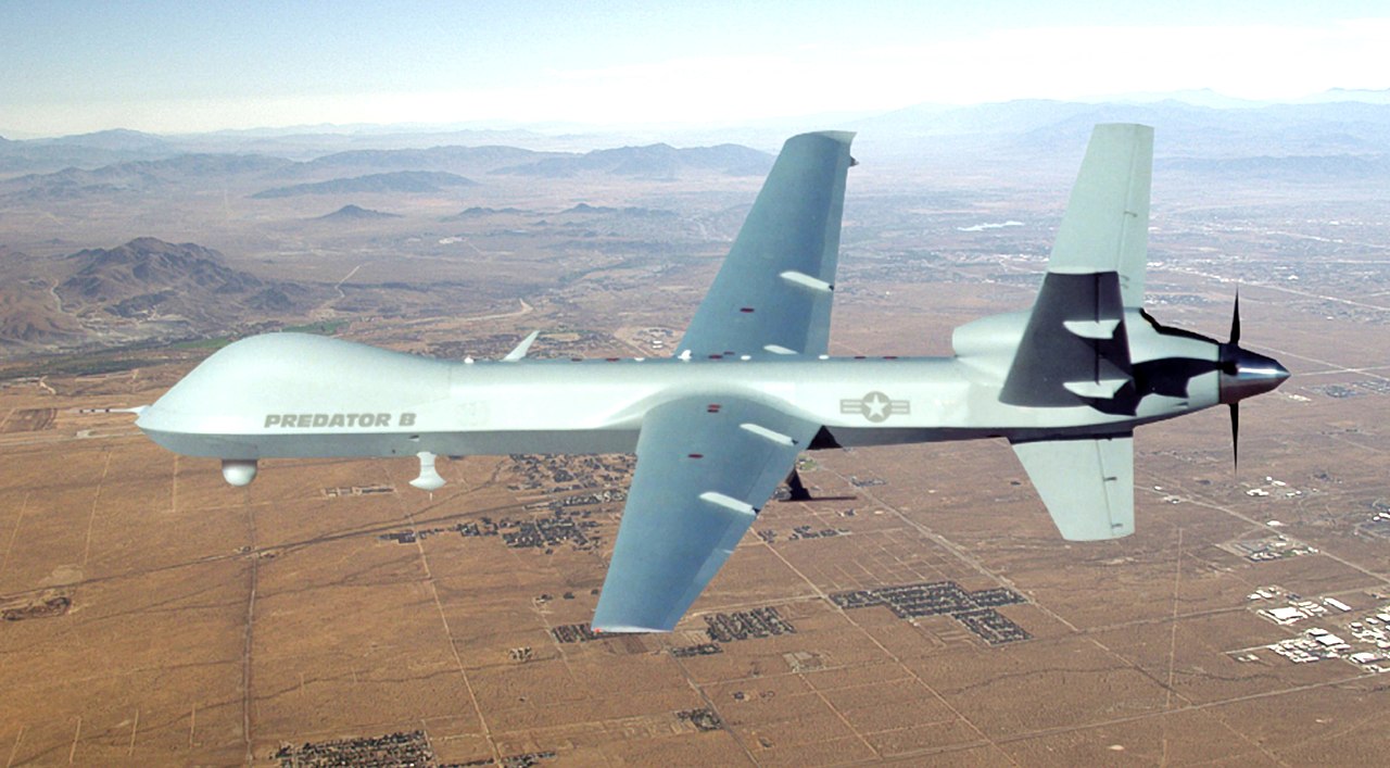
The wake generated by the fuselage will influence the aerodynamic performance of a pusher propeller because it ingests air that has been /altered by upstream boundary-layer growth and, in some cases, by regions of separated flow. The principal aerodynamic consequence is a distortion of the inflow profile across the propeller disk, with the inner region typically experiencing a significant velocity deficit. The upshot is a reduction in the effective mass flow rate through the propeller, along with changes to the local angle of attack on the blades. In severe cases, ingesting a fuselage wake can introduce unsteady turbulent structures into the flow, potentially degrading propeller performance and increasing noise.
There are few direct measurements that compare the performance of pusher propellers versus that of tractor propellers under the same or similar operating conditions. Fred Weick alludes to wind tunnel tests conducted by the Royal Aircraft Establishment (RAE) in 1922. The results, which are summarized in the figure below, suggest that even with relatively large fuselage sizes compared to the propeller diameter, the effects on maximum propulsive efficiency of a pusher versus a tractor propeller are minimal, perhaps on the order of 2%. Nevertheless, the wide range of potential fuselage shapes and downstream wake profiles that could be encountered in practical design indicates that some modeling effort is warranted to better understand the magnitude of the possible interference effects.
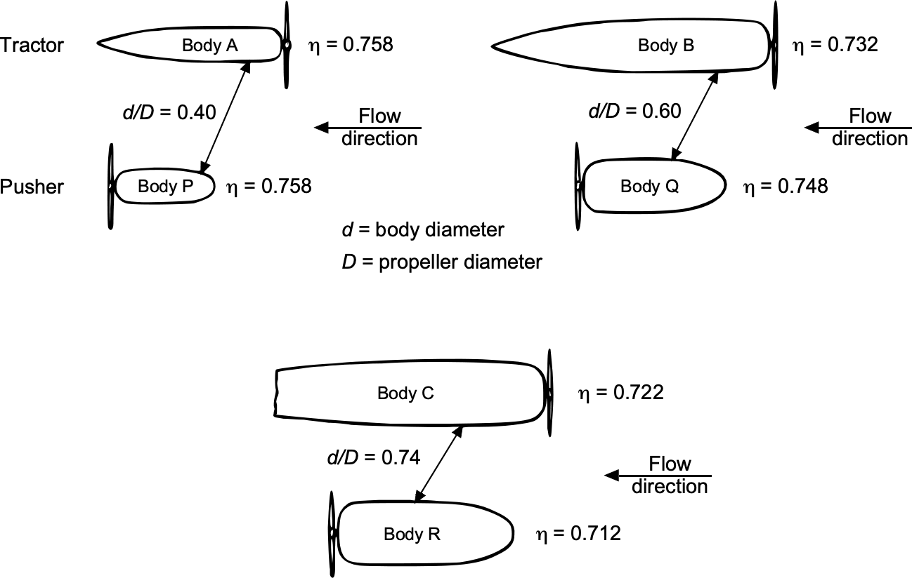
Flow Model
Consider a flow model of a pusher propeller, as shown in the figure below, where the inflow into the propeller disk is composed of two concentric zones:
- An inner disk of radius
 that is subject to a velocity deficit
  , i.e.,
  . The parameter
  is a characteristic wake width or spread parameter, typically comparable to the fuselage diameter.
 - An outer annular region from
 to
to  that is exposed to undisturbed freestream flow, i.e.,
  .
.
In this model, each region is treated as an independent actuator disk segment, where  and
and  denote the inner and outer areas, respectively. Assume both regions have the same average induced velocity at the plane of the propeller.
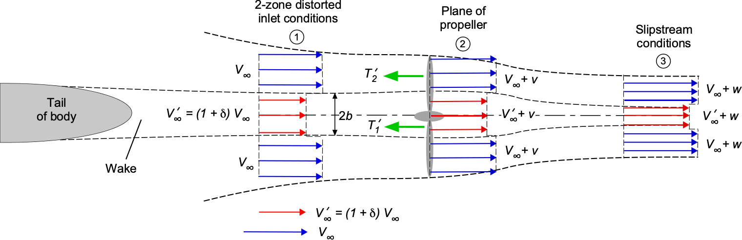
Thrust
(121) 
Therefore, the total thrust is
(122) 
Notice that =  , so this previous result becomes
(123) 
The corresponding thrust in the clean inflow case (no velocity deficit) is
(124) 
and so the thrust ratio (distorted inflow versus clean) is
(125) 
which for  , i.e., a propeller at typical thrust levels in the normal working state, becomes
(126) 
Power
Now, consider the power required. The average velocity through each region of the disk is
(127) 
The thrust in each region is given by Eq. 121, so the total power required becomes
(128) 
Substituting and expanding gives
(129) 
so that
(130) 
In the limit as , the second term is small and may be neglected, giving
(131) 
The ideal (clean inflow) power required is
(132) 
so the power ratio (distorted inflow versus clean) is
(133) 
Because  and
and  , then the power ratio becomes
(134) 
Efficiency
Finally, the propulsive efficiency with inflow distortion is defined in the conventional way using
(135) 
From the previous results, then
(136) 
Therefore,
(137) 
Multiplying out and keeping only first-order terms gives
(138) 
(139) 
showing that the change in efficiency increases proportionately to the wake velocity deficit , and the area ratio  , i.e., the portion of the propeller disk immersed in the wake.
The apparent increase in propulsive efficiency given by Eq. 139 is a consequence of the idealized assumptions of the actuator disk model, including uniform induced velocity and no swirl. Physically, such an effect could occur because the inner part of the propeller, which generates little propulsive work, consumes less power because of wake deficiency and lower dynamic pressure. However, inflow distortion near the hub may introduce additional losses not accounted for in this analysis.
Low Reynolds Number Propellers
Low Reynolds number propellers are designed to perform efficiently in flow regimes characterized by Reynolds numbers based on the blade sectional chord at 75% radius, typically below 105. Such operating conditions are generally found on small airplanes, UAVs, and drones. In this regime, the blade sectional drag values are higher than at chord Reynolds numbers above 106, which significantly impacts the thrust and lowers the overall propulsive efficiency of the propeller.
As the Reynolds number decreases below one million ( ) and viscosity begins to outweigh inertia in the flow, the lift and drag characteristics of airfoil sections undergo profound changes. The data in the figure below show the profound effects of operating airfoils at lower Reynolds numbers, ranging from 20,000 to 3,000,000 (three million). At the highest Reynolds number of
  , the lift coefficient varies almost linearly with the angle of attack, which is typical of airfoil behavior at higher Reynolds numbers. However, as the Reynolds number decreases below a million, the lift and drag curves become significantly more rounded and eventually become nonlinear for variations in the angle of attack. Indeed, these effects start to become pronounced even at Reynolds numbers of 500,000.
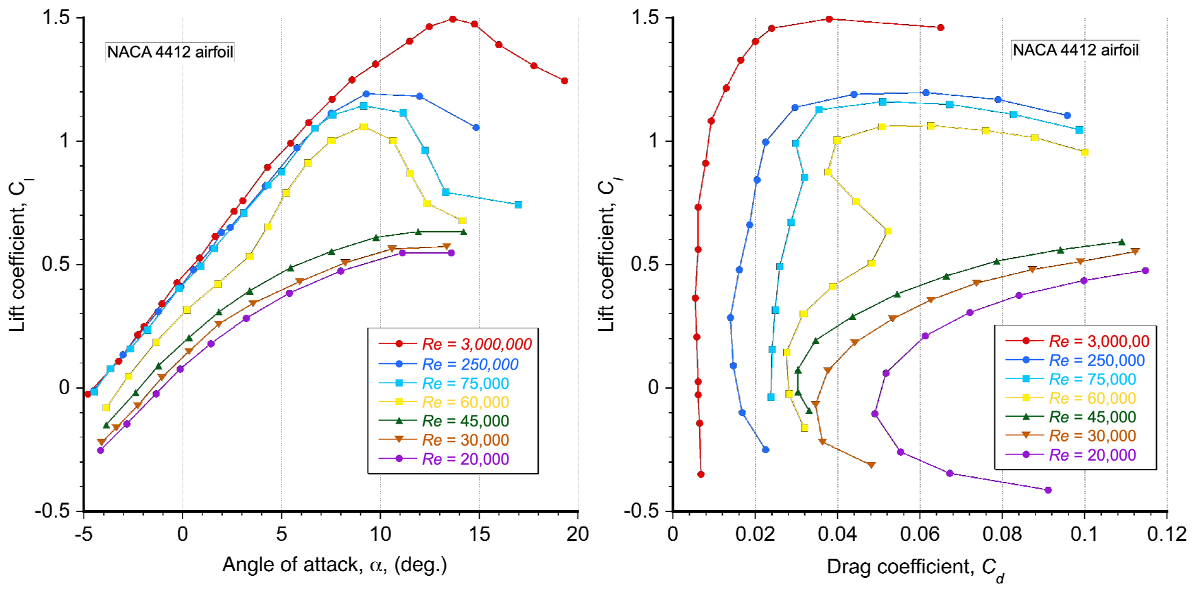
The corresponding drag polar for these conditions provides another helpful way to summarize the effects of the Reynolds number on the aerodynamic characteristics. Notice again the profound effects of reducing the Reynolds number below 500,000, which deleteriously affect the lift-to-drag ratio, especially below 50,000. For extremely low Reynolds numbers of less than  , lift-to-drag ratios of less than 5 are expected, at least with “conventional” airfoil sections.
Therefore, the impact of these airfoil section effects on propeller performance at low chord Reynolds numbers is profound. For example, the figure below illustrates the efficiencies of a two-bladed propeller at “full scale” and two smaller ones operating at lower tip Reynolds numbers based on average chord. Notice the marked drop in maximum efficiency at lower Reynolds numbers, as well as the range of Reynolds numbers over which the system can operate efficiently. Most of these effects on propulsive efficiency are primarily related to the higher sectional drag coefficient values at these low Reynolds numbers.[15] However, there is also a reduction in maximum sectional lift values, which limits thrust production. These considerations are essential for propeller applications in most UAVs and drones, which can expect maximum propulsion efficiencies of 50% to 60%, rather than 80% or higher for “full-scale” propellers.
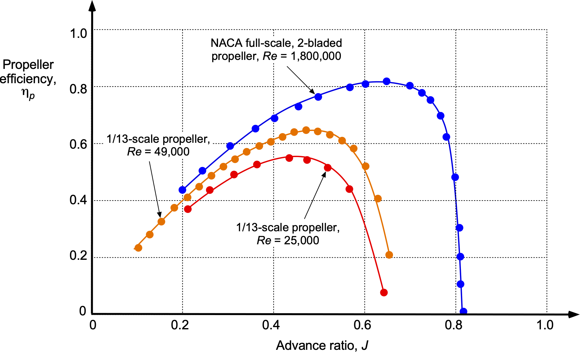
Unique low-Reynolds-number airfoil designs are typically employed to minimize sectional drag on smaller propellers, much as those used on fixed wings, but these designs must be carefully tailored. A larger solidity (blade area) also assists in generating the necessary thrust under these conditions, perhaps at the expense of some other losses in propulsive efficiency. Designing low-Reynolds-number airfoils suitable for propellers typically involves utilizing advanced computational fluid dynamics (CFD) simulations to analyze and optimize their performance. These simulations enable engineers to understand the flow behavior around propeller blades and refine design parameters. Wind tunnel testing is essential for validating the design assumptions and performance predictions.
Selecting Propellers for a Drone
Selecting the correct propeller(s) for a UAV or drone involves several interrelated factors, including the drone’s size, weight, aerodynamic and motor characteristics, and the desired flight performance, such as airspeed, range, and endurance. A VTOL-capable drone may use a separate set of propellers for lifting and another for propulsion, i.e., a hybrid concept. In this setup, the lifting propellers are switched off in forward flight, and a conventional fixed wing generates the lift to overcome the drone’s weight. In some cases, propellers may be used for both lifting and propulsion, as in a tiltrotor or tilting wing concept, which requires further compromises in selecting the best propeller. The assumption is that such propellers are of fixed pitch only, so the selected propeller(s) will inevitably be a compromise.
Steps for Propeller Selection
The following are the basic steps to select the appropriate propeller(s) for low-Reynolds-number operation. Inevitably, without access to a test rig and a wind tunnel, the process will involve trial and error, as well as sound judgment and a degree of common sense. Fortunately, at this smaller scale, propellers are inexpensive, allowing the final decision to be made through flight testing with a selection of different propellers until the best performance is achieved.
- Propeller diameter. To determine the propeller requirements, consider the drone’s weight, aerodynamic efficiency (e.g., lift-to-drag ratio), estimated motor specifications, battery type, voltage, and desired flight characteristics. Heavier drones require larger-diameter, higher-pitch propellers to generate sufficient thrust to overcome their drag. A VTOL drone requires sufficient thrust from its lifting propellers to overcome its own weight and maintain lift.
- Calculate the thrust and power requirements. A thrust-to-weight ratio of about 2:1 is necessary for good hovering, forward flight, and maneuvering performance for a quadcopter drone. For example, if a drone has a mass of 1 kg, the design thrust must be capable of carrying 2 kg, e.g., 500 g per motor and propeller for a quadcopter. The power requirements can be estimated using the momentum theory, starting from an initial estimate of the needed propeller diameter.
- Match to motor. Match the initial size and pitch of the propeller to the motor’s recommended range, taking into account the motor’s power or “KV rating.” Different propellers can dramatically affect the drone’s speed, maneuverability, and other flight characteristics.
- Establish the type of propeller. A propulsive propeller will require significantly less thrust than the drone’s weight, depending on the drone’s lift-to-drag ratio. The goal is to achieve the highest level of propulsive efficiency at the propeller’s operating value for a given combination of required thrust, propeller rpm or rps, and airspeed. To this end, propeller charts., i.e., versus , versus and versus should be consulted. The speed-power coefficient, , should be evaluated.
- Review small-scale propeller measurements. They are available in chart form and as data files. They cover a comprehensive range of propellers suitable for drones. Measurements are available in the static thrust condition (i.e., hover) and forward flight over a range of values. Remember that small propellers have relatively low thrust-producing efficiencies, ranging from 50% to 60%, which impacts flight duration for a given battery charge.
- Consult the motor specifications. The motor’s datasheet may recommend a propeller size (diameter) and pitch. Manufacturers often provide a range of suitable propellers for their motors. It is usually wise to stay within the recommended ranges, although other propellers may also be appropriate.
- Decide on the propeller geometry. Propellers are specified by diameter and pitch. For example, a propeller marked as 20 x 14 means it has a diameter of 20 inches and a helical pitch distance of 14 inches; the propeller could also be specified in cm units. Propellers come in quantum sizes such as 12 inches, 14 inches, etc. Lifting (hovering) propellers will have relatively low pitches, whereas propulsive propellers will have higher pitches. The faster the drone must fly, the higher the propeller pitch needed for good propulsive efficiency.
- Decide on the propeller material. Plastic propellers are lightweight and inexpensive but less durable. Carbon fiber propellers give better aerodynamic performance but are significantly more expensive. It is often a good choice to buy and test three inexpensive propellers initially, perhaps with higher and lower pitches than the first choice, before settling on a carbon fiber propeller.
Hovering (Static Thrust) Propeller
Propellers generally have lower static thrust or hovering efficiency compared to helicopter rotors, partly because of their typically higher disk loadings and non-optimal blade designs. The power requirements can be decomposed into an induced component, which depends on thrust, and a profile component, which is constant and independent of thrust.
Induced Power
From momentum theory, the induced velocity at the propeller’s disk is
(140) 
where is the thrust required. The ideal induced power required is
(141) 
Expressing this result in terms of the propeller thrust coefficient, i.e.,  , gives
(142) 
Therefore, the ideal induced power coefficient using the propeller definition is
(143) 
Accounting for induced losses with the induced power factor  , the actual induced power coefficient is
(144) 
Profile Power
The profile power is the power required to overcome the aerodynamic drag of the propeller blades as they rotate through the air, independent of any thrust generation. For a propeller in hover, assuming constant blade chord  , constant section drag coefficient
  , the differential profile power on a blade segment at radius is given by
(145) 
Multiplying by the number of blades and integrating from the root ( ) to the tip () yields the total profile power, i.e.,
(146) 
The nondimensional profile power coefficient is defined as
(147) 
and substituting  and , this becomes
(148) 
The solidity of the propeller is
(149) 
ans substituting into the expression for  gives
gives
(150) 
Total Power
Finally, the total power coefficient for hovering flight using the modified momentum theory is
(151) 
Alternatively, the power coefficient can be written in terms of the figure of merit,  , as
, as
(152) 
As shown in the power polar in the figure below, with suitable values for  and (or ), the modified momentum theory can provide good predictions of hovering performance. The low Reynolds number, combined with the typical (and excessive) spanwise blade twist and non-optimal chord distribution used on these propellers, generally results in relatively poor hovering performance. In this case, = 1.35 and = 0.2 (
  0.5) gives good agreement with these measurements. Notice that increasing propeller pitch produces more thrust for the same rpm; the resulting measurements then move up the curve to higher values of and . The effects of Reynolds number, combined with rpm, slightly increase thrust and reduce power at higher values of rpm.
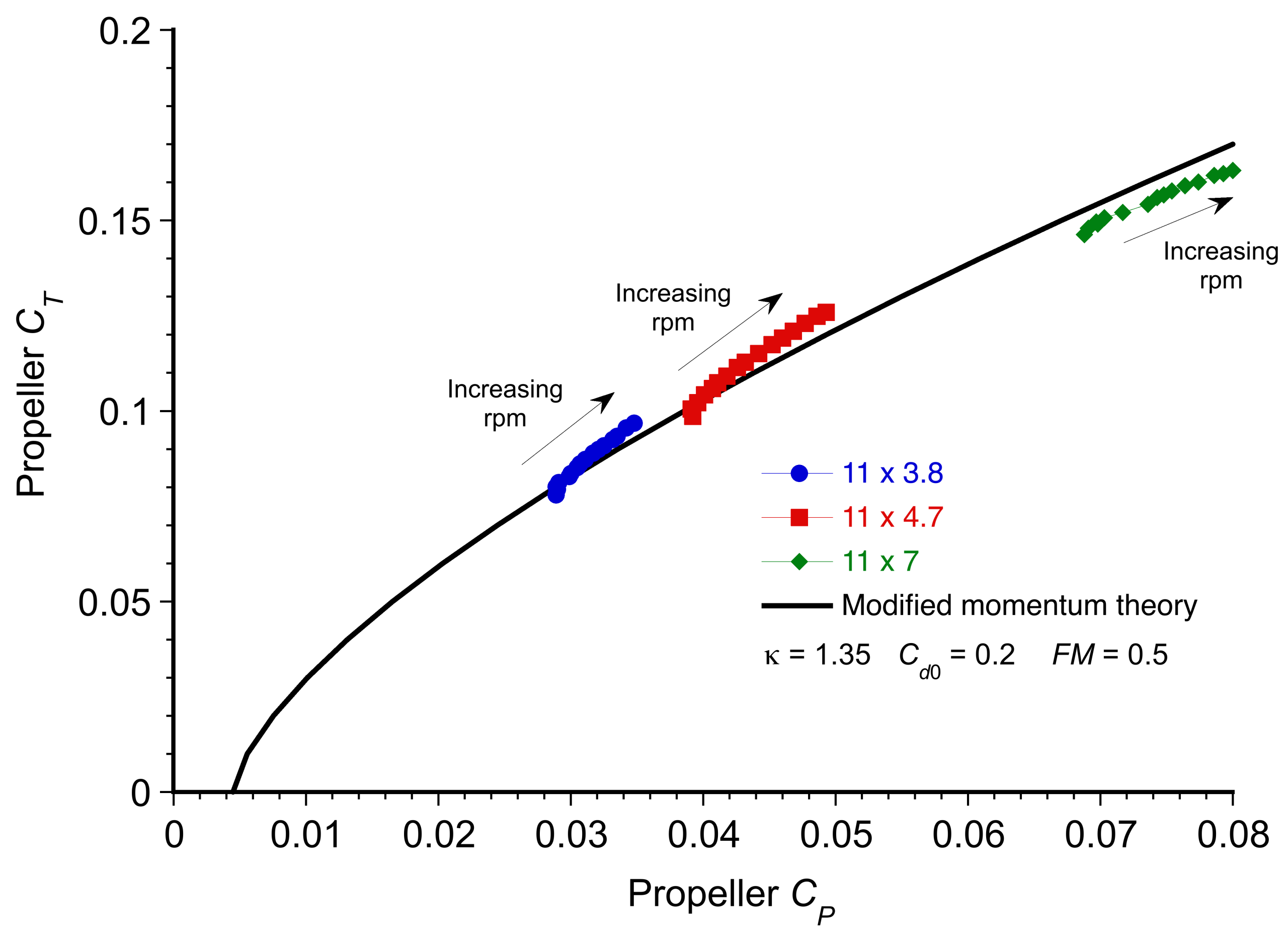
Worked Example #3 –Drone in hovering flight
A VTOL quad-rotor drone weighs 7.5 kg at takeoff, including the battery, camera, and other components. Estimate the size of the propellers and motors needed. Assume MSL ISA conditions.
Show solution/hide solution.
- As a general rule of thumb, the thrust required from the propeller(s) must be enough to carry 7.5 kg 2 = 15 kg to ensure sufficient takeoff and maneuver performance. For example, for a quadcopter, each motor must be attached to a propeller to provide enough thrust to overcome 3.75 kg, i.e., a weight of 36.8 N.
- Estimate the propeller’s diameter and pitch to produce the required thrust. The thrust equation is
 , where in this case = 36.8 N (thrust per propeller), = 0.12 (nominal thrust coefficient for a low pitch propeller as shown in the figure above), = 1.225 kg/m
 (standard sea-level air density), = rpm/60 = 8,880/60 (rotations per second), = propeller diameter (m). Rearranging to solve for gives
![\[ d = \left( \frac{T}{C_T \, \varrho_{\infty} \, n^2} \right)^{\dfrac{1}{4}} \]](https://eaglepubs.erau.edu/app/uploads/quicklatex/quicklatex.com-35c1d49424ce21fd77e905afc928684e_l3.svg "Rendered by QuickLaTeX.com")
and substituting the values gives
![\[ d = \left( \frac{36.8}{0.12 \times 1.225 \times \left(\dfrac{8,880}{60}\right)^2} \right)^{\dfrac{1}{4}} = 0.33 \text{ m} =12.9 \text{ inches} \]](https://eaglepubs.erau.edu/app/uploads/quicklatex/quicklatex.com-55e2a95579adbdf1bd55b803f4b61188_l3.svg "Rendered by QuickLaTeX.com")
Propellers are usually only available in quantum sizes, so the next size up will be 13 or 14 inches.
- The momentum theory can be used to estimate the net power, which will be
![\[ P_{\rm req} = \frac{N_r}{FM} \frac{T^{3/2}}{\sqrt{2 \varrho_{\infty} A}} \]](https://eaglepubs.erau.edu/app/uploads/quicklatex/quicklatex.com-c6e6b7a54f1fd8f3d05a65b9202861e6_l3.svg "Rendered by QuickLaTeX.com")
where
 is the number of rotors (= 4 in this case), , and the figure of merit, , for a small rotor can be assumed to be 0.6. Inserting the numbers gives
![\[ P_{\rm req} = \frac{4}{0.6} \frac{33.8^{3/2}}{\sqrt{2 \times 1.225 \times \pi \times 0.33^2/4}} = 3.25 \text{ kW} \]](https://eaglepubs.erau.edu/app/uploads/quicklatex/quicklatex.com-9680597c52a162019e9a7cccf2e451d2_l3.svg "Rendered by QuickLaTeX.com")
so about 800 W per motor.
- Select the motor in the 800 W power class. Motors are marketed using a kV (or KV) rating, and most also recommend a specific battery requirement. For example, a motor may have an 800 KV rating, which means it will spin at 800 rpm per Volt. If it is supported by an 11.1-Volt LiPo battery, it will spin up to 8,800 rpm. A 200-kV to 400-kV motor will likely be the most suitable choice in this case.
- The motor’s datasheet may also suggest a range of propeller sizes and helical pitches that fully absorb the motor’s power and give good propulsive efficiency. A propeller for good hovering performance typically has a helical pitch of about 3 to 4 inches, but this depends on the required thrust.
- Test the drone with the selected propeller(s) to ensure proper operation. If necessary, propellers of a slightly different pitch may be needed. Suppose a test stand with a load cell or even a digital spring balance is available. In that case, thrust and battery energy consumption can be measured with different propellers to determine the most suitable one before the first flight tests. Remember that the best lifting propellers will have low helical pitch values.
- While more detailed performance calculations may ultimately be required, the steps here outline a rapid method for sizing the propellers.
Propulsion Propeller
Selecting a propeller for a drone to meet its propulsion requirements must be performed more rigorously and requires access to propeller charts, specifically the thrust coefficient versus advance ratio , the power coefficient versus , and the efficiency versus . Such charts may come from wind tunnel tests or calculations using a propeller model (code). Propulsive propellers for drones, with their high rpm values and lower airspeeds (compared to a conventional airplane), operate at relatively low values, typically less than unity.
The figure below shows wind-tunnel measurements for a small-scale propeller with three pitch values under consideration to meet propulsive requirements. At low values of , the propeller blades may stall due to excessive pitch relative to the incoming airflow. As airspeed builds and increases, the blade angles of attack decrease, and the propeller starts to produce useful thrust, also with increasing propulsive efficiency. At some point, the propeller reaches its maximum efficiency. Beyond this, for a given rpm, the blade section angles of attack continue to decrease, which reduces both the lift produced by the blades and the net thrust from the propeller. Eventually, the thrust reduces to zero, and at sufficiently high for a given blade pitch, the propeller starts to generate negative thrust, thereby creating drag.
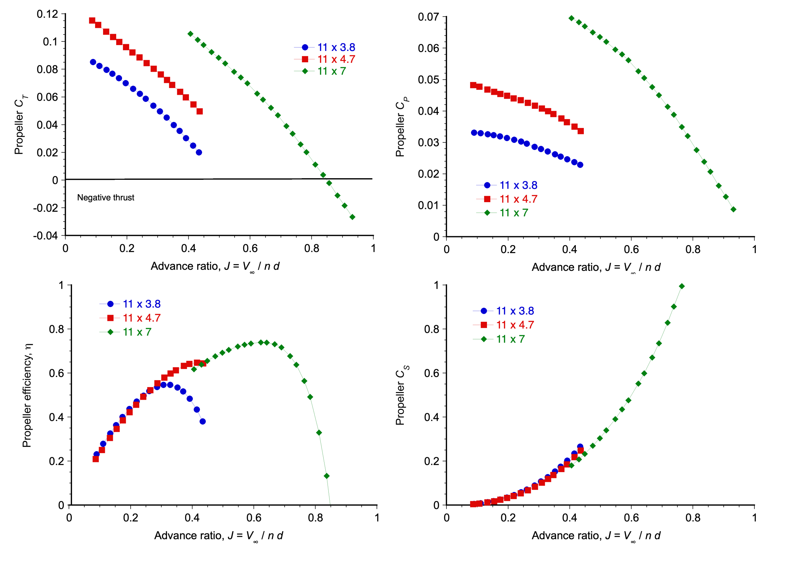
 .
.When selecting a specific fixed-pitch propeller, the goal is to operate it at or near its optimal propulsive efficiency. The advantage of non-dimensional coefficients, including the speed-power coefficient, is that the results can scale to different propeller diameters, provided the Reynolds numbers do not change significantly, possibly up to 20%. Inevitably, oversized propellers will have to operate at values of that are too low to be efficient. In contrast, smaller propellers will have to operate at much higher values of to provide the required thrust. Higher blade pitch values will increase the value of , at which the maximum propulsive efficiency is obtained. The process is inevitably iterative, based on the power required for flight (and hence the drone’s drag), with the final propeller pitch a compromise. While it is a point design, it should also have some operating margins in terms of efficiency over a range of airspeeds. Besides , the use of the coefficient helps ensure that the selected propeller is matched to the powerplant and aircraft that it powers.
Worked Example #4 – Propeller selection for a drone in forward flight
Consider selecting a propeller for a drone with a motor turning at 7,000 rpm and delivering 8 kW of power. The required cruise airspeed is 45 mph. The initial choice is an 11 x 3.8-inch pitch propeller, with the 11-inch diameter based on a geometric constraint. Assume MSL ISA conditions and the availability of propeller performance data.
Show solution/hide solution.
The first step is to compute the speed-power coefficient, which is defined as
(153) 
Substituting the known values, = 1.225 kg/m , = 20.12 m/s, = 8,000 W, and = 7,000/60 = 116.67 rps, gives
(154) 
Using the curves and the propeller efficiency curves, a speed-power coefficient of approximately 0.52 corresponds to a 7-inch pitch propeller that would be operating near its peak propulsive efficiency. Notice that the shaded zones represent where the values of and are compatible.
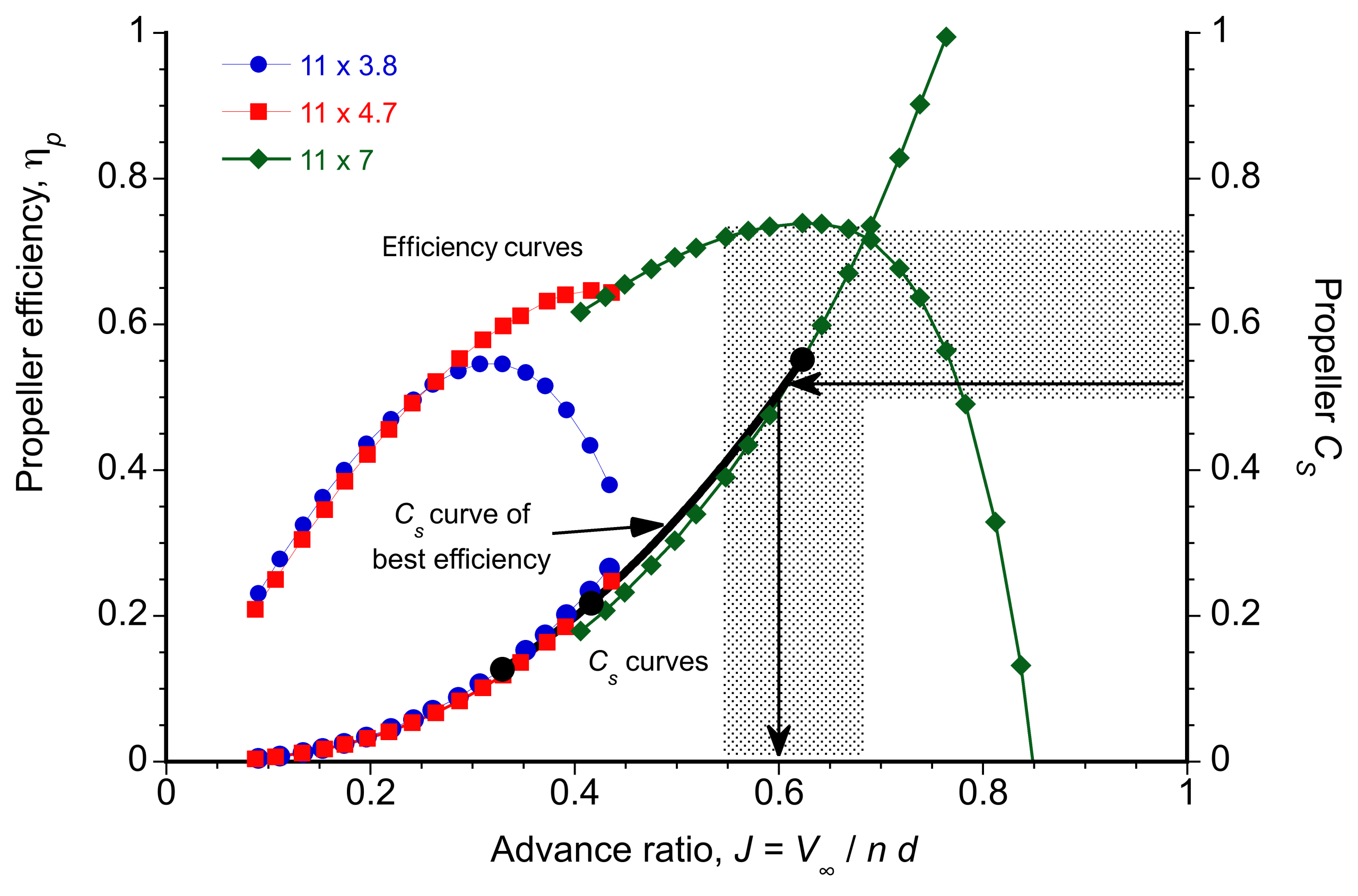
The associated advance ratio for best efficiency at this pitch is approximately = 0.60. The diameter can now be determined using
(155) 
This result suggests that an 11.3 x 7-inch propeller would be a better match for this motor than the initially chosen 11 x 3.8-inch propeller. A standard 11 x 7-inch fixed-pitch propeller will closely meet this specification.
Summary & Closure
Propellers are an effective and robust means of generating thrust, making them widely used in aviation across various propulsion systems. Fixed-pitch propellers, while straightforward and lightweight, have inherent limitations in their efficiency across different flight conditions. Variable-pitch and constant-speed propellers expand the operational range, allowing for better efficiency at various speeds and altitudes, though they come with increased mechanical complexity, weight, and cost. Whether paired with piston, turboshaft, or electric motors, correctly matching the propeller to its specific powerplant is crucial for achieving optimal performance.
A key trend in modern airplane design is the shift toward propellers with smaller diameters and more blades. This configuration helps reduce blade tip speeds, minimize noise, and improve efficiency. Advances in composite materials, such as Kevlar and carbon fiber, have further transformed propeller design. These materials enable thinner, swept blades that enhance aerodynamic efficiency at higher tip Mach numbers and flight speeds while reducing weight, vibration, and acoustic footprint. Despite these innovations, wooden propellers are still used for low-performance airplanes because of their cost-effectiveness and ease of manufacturing.
For UAVs and drones, propeller selection plays a crucial role in overall efficiency, endurance, and mission effectiveness. Fixed-pitch propellers are typically preferred because of their simplicity and reliability; however, they require careful optimization to achieve optimal performance. The relationship between blade pitch, advance ratio, and rotational speed must be fine-tuned to ensure efficient thrust production across various flight conditions. Non-dimensional coefficients, such as the power-speed coefficient, help scale performance across different propeller sizes, but trade-offs are inevitable. The iterative nature of propeller design means that achieving the right balance between thrust production and power consumption is essential. Ultimately, the goal is to develop propellers that maintain high efficiency across a range of operating conditions while meeting noise, weight, and performance constraints. As UAV and drone technology advances, so will propeller innovations, pushing the boundaries of aerodynamic efficiency, power optimization, and operational versatility.
5-Question Self-Assessment Quickquiz
For Further Thought or Discussion
- Is using a fixed-pitch or constant-speed propeller for a UAV desirable? Discuss.
- Why does using a swept blade on a propeller generally help give the propeller better efficiency?
- Discuss the factors that may influence the design of a propeller blade, including material selection, shape, and angle of attack.
- Explain the concept of propeller slipstream and its influence on the overall aerodynamic performance of an aircraft. How does the slipstream interact with other aircraft components?
- Explain how tip speed affects propeller noise and efficiency. What design considerations are made to optimize tip speed within acceptable limits?
- Explain the phenomenon of propeller torque and its effect on aircraft handling. How do pilots and designers compensate for torque effects during flight?
Other Useful Online Resources
To learn more about propellers, check out these helpful online resources:
- Ever wonder how an airplane propeller is made? Take a tour of Hartzell Propeller to learn how propellers work and how they are made.
- “The Propeller Explained” is a documentary film.
- World’s Largest Wooden Propeller Factory: How It’s Made.
- Props to Alaina: The Art of Airplane Propellers.
- How Sensenich Wooden Props are made.
- Apparently, this is the only video you need to understand airplane propellers. It’s good, but there is more to learn.
- “Airplane Propellers: Principles and Types” is a World War II-era U.S. War Department training film.
- In 2022, students from the University of Maryland built a flying quadrotor drone based on the aerial screw design. Still, it only had a novelty value compared to modern quadrotor designs. ↵
- A steam engine of the era would have been far too heavy (boiler, engine, condenser, fuel, water, etc.) and with too little power to be of any aeronautical use. ↵
- Glauert, H. (1935) "Airplane Propellers." In: Durand, W.F., Ed., Aerodynamic Theory, Vol. IV, Division L, Springer, New York, 169–360. ↵
- . An excellent analogy for this concept is a continuously variable transmission in an automobile. ↵
- The blade twist distribution is fixed and cannot be varied. ↵
- The actuator disk is equivalent to an infinite number of blades. ↵
- rpm = revolutions per second; rps = revolutions per minute. ↵
- Aspects of Rankine's propeller theory were published in various sources, including Rankine, W. J. M., "On the Mechanical Principles of the Action of Propellers," Transactions of the Institute of Naval Architects, Vol. 6, pp. 13-39, 1865. ↵
- Froude, R. "On the Part Played in Propulsion by Differences in Fluid Pressure," Transactions of the Royal Institution of Naval Architects, 30, 390, 1889. ↵
- The boss is simply the part of the propeller that is used to attach it to the engine shaft or gearbox. ↵
- However, it should be noted that the definitions of and are different from those used for helicopter rotors. ↵
- In a free-turbine turboprop, the propeller is driven by a power turbine that is not mechanically connected to the gas generator. ↵
- Weick, F. E., Aircraft Propeller Design, McGraw-Hill Book Co., Inc., New York and London, 1930. ↵
- The reciprocal of the coefficient was used by Drzewiecki. See: Drzewiecki, S., Théorie Générale de l'Hélice Propulsive, Gauthier-Villars, Paris, 1920. This form, however, spans a wide range of values, making it impractical to use. ↵
- Although some additional losses come from the wake, which experiences a higher fraction of losses from the thicker boundary layers trailed into the wake and increased turbulence from shear. ↵
