35 Potential Flow Theory
Introduction[1]
Potential flow methods utilize the mathematical principle that the gradient of a scalar field is a vector, such as a velocity field. A potential flow assumes the aggregate of an incompressible, irrotational, and inviscid fluid motion, i.e., which is called an “ideal” flow. These assumptions could be considered significant, if not sweeping, approximations to an actual or “real” flow, in general. However, many interesting and practical flows can be regarded as potential flows for analysis and prediction. More importantly, such assumptions are also used in developing various aspects of airfoil and wing theories, which will be considered in the following chapters, and for which studying the fundamental elements of potential flows is a necessary prerequisite.
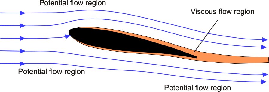
The use of the term “irrotational” in the previous paragraph requires some elaboration. An irrotational flow is mathematically stated as  , i.e., the curl of the velocity field is zero. This condition implies that the fluid elements do not undergo any spin or rotation, thereby eliminating viscous shear forces and precluding the generation of turbulence. Additionally, the absence of viscosity (an inviscid flow) renders the creation of shear stresses physically impossible. These assumptions significantly simplify the flow analysis, and the inviscid assumption is particularly valid for analyzing external flows far from solid boundaries, i.e., outside the boundary layers or wakes that may be generated. For example, the flow around an airfoil, as shown in the figure below, is predominantly a potential flow away from the airfoil’s immediate surface. For clarity, the extent of the viscous flow region is exaggerated for illustration purposes, and the boundary layer is very thin relative to the thickness of the airfoil.
Consequently, studying potential flows provides an insightful and tractable framework for predicting and understanding a range of flow problems. For such problems, exact analytical solutions are often possible, yielding valuable insights into the fundamentals of fluid dynamics. Potential flows are foundational in many classical aerodynamic theories, including thin airfoil theory, lifting-line theory, and lifting-surface theory, which are widely used to model and analyze airflow behavior around bodies, airfoils, and wings. Numerical methods, known as surface-singularity or panel methods, can further extend the applicability of potential flow theory, including to complete airplane shapes, making it a valuable approach in flight vehicle design and numerous other engineering applications.
Learning Objectives
- Understand the principles of incompressible, irrotational, and inviscid fluid motion, i.e., potential flows.
- Become familiar with elementary potential flow solutions, including uniform flow, source/sink flows, doublets, and vortices.
- Learn how to combine elementary solutions to construct more complex potential flow fields through linear superposition.
- Use complex variable methods to represent and analyze two-dimensional potential flows.
- Understand the method of conformal mapping and how it is used to transform simple potential flows onto more useful geometries, such as airfoil shapes.
- Be aware of the Prandtl-Glauert compressibility correction and its application in approximating subsonic compressible flow effects using incompressible potential flow solutions.
History
The origins of the potential flow theory can be traced back to the 18th century, with contributions from Daniel Bernoulli and Leonhard Euler. Bernoulli introduced an equation to relate velocity and pressure in inviscid, incompressible fluids; the famous Bernoulli principle, also known as the Bernoulli equation, is a cornerstone of fluid mechanics. Euler expanded on this work by deriving the equations of motion for inviscid flows and introducing the velocity potential, a scalar function whose gradient gives the fluid velocity. Pierre-Simon Laplace further formalized these ideas and contributed to the development of superposition methods for combining elementary flow solutions, such as sources, sinks, and vortices, to model more complex and interesting flows.
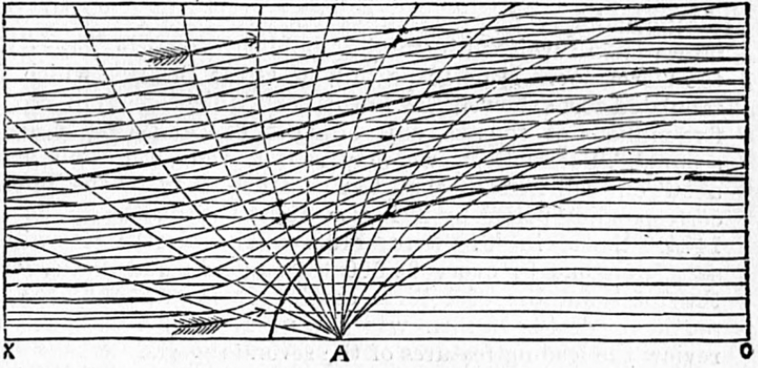
In the 19th century, significant advancements in potential flow theory included the mathematical formalization of streamlines. George Stokes published the first and most complete exposition[2] in 1842. William Rankine analyzed the flow patterns around simple geometries[3] using a potential flow method, while Hermann von Helmholtz formulated the conservation of vorticity in inviscid flows, a concept critical to understanding the concept of circulation and lift generation. Rankine was interested in the flows around ship hulls, for which a potential flow solution provided much insight. The figure below illustrates his calculations for an oval “half-body,” which Rankine called an “Oögenous Neoïd.”
However, the limitations of potential flow were also exposed, most notably by Jean le Rond d’Alembert‘s so-called paradox, which showed that the assumption of a potential flow predicts zero drag on symmetric bodies. This paradox highlighted that additional flow characteristics, specifically the action of viscosity, were necessary to reconcile the discrepancies between predictions and experiments. Despite these limitations, potential flow quickly became a central tool for analyzing fluid motion.
The early 20th century saw the application of potential flow theory to airfoils and wings. Frederick Lanchester played a pivotal role in integrating the concept of circulation into the understanding of lift generation. Martin Kutta and Nikolay (Nikolai) Joukowsky independently developed theories that mathematically linked circulation to lift. These contributions introduced the idea of what is now known as the Kutta condition, which models the smooth flow observed at an airfoil’s sharp trailing edge. Ludwig Prandtl built on this work by developing the thin airfoil and lifting-line theories, providing the first models to predict the lift and drag of two-dimensional airfoils and three-dimensional wings. These theories allowed engineers to design and analyze airfoils and wings with reasonable predictive accuracy despite the incompressible and inviscid flow assumptions.
Later in the 20th century, potential flow theory was extended to compressible flows, resulting in techniques such as the Prandtl-Glauert transformation for subsonic flows. Numerical methods, such as panel methods, were introduced in the 1970s to solve potential flow problems for more complex geometries, including aircraft fuselages and wings. While potential flow cannot predict viscous effects, flow separation, or turbulence, it remains foundational for understanding basic fluid behavior. It also serves as a starting point for learning about more advanced models, making it an indispensable part of fluid mechanics in an engineering education.
Definition of a Potential Flow
Potential flow methods use the mathematical principle that the gradient of a scalar field is a vector field. For example, if  is a scalar field, then the gradient
  (or grad
  ) is given by
(1) 
The vector operator  (called nabla or del) is defined as
(2) 
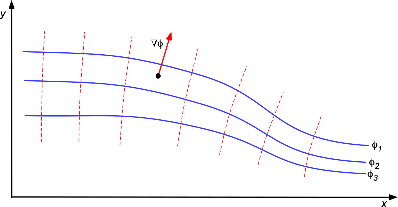
Physically, is the normal (perpendicular) to the surface defined by  = constant, which is called an equipotential surface, as illustrated in the figure below.
Potential Flow Equations
Potential flow methods in aerodynamics simplify the governing equations of fluid motion by assuming inviscid and irrotational flow, allowing the velocity field to be expressed as the gradient of a scalar potential function. In an incompressible flow, this approach leads to Laplace’s equation, a linear, analytically tractable form of the governing equations of fluid motion. For compressible flow, however, the same assumptions lead to a nonlinear governing equation known as the full potential equation. Derived from the Euler and continuity equations, the full potential equation accounts for variations in velocity, pressure, and density, and forms the basis for more advanced models of subsonic, transonic, and supersonic flow.
Full Potential Equation
For a compressible, inviscid flow, the governing equations are
(3) 
and
(4) 
If it is assumed that the flow is irrotational, the flow velocity can be written as the gradient of a scalar potential function, i.e.,
(5) 
Substituting this into the momentum equation gives
(6) 
Using the identity
(7) 
then the unsteady form of the Bernoulli equation in differential form is obtained, i.e.,
(8) 
Assuming isentropic flow, the pressure and density are related by  , where
  is the local speed of sound. Therefore,
(9) 
which defines a compressible enthalpy function  , leading to
(10) 
To eliminate  , the implicit dependence of density on the potential function through the Bernoulli relation can be invoked. Differentiating this relation allows to be expressed as a function of and its derivatives. Substituting and simplifying yields the full potential equation, which is a second-order nonlinear PDE for the velocity potential , i.e.,
(11) 
Alternatively, in expanded form and written for compressible unsteady flows, it takes the form
(12) 
where  is the magnitude of the velocity and is the local speed of sound. This latter equation retains all essential compressibility effects and applies to subsonic, transonic, and supersonic regimes, but still assumes irrotational and inviscid flow. It also serves as the starting point for developing various simplified models, such as the transonic small disturbance (TSD) equation and the linearized potential flow equations.
TSD & Wave Equations
The transonic small disturbance (TSD) equation is a variation of the full-potential equation for small disturbances, which can be written as
(13) 
For steady flows, this previous equation reduces to
(14) 
The TSD equation is nonlinear and foundational in computational fluid dynamics (CFD). Further, assuming small disturbances reduces the TSD equation to a wave equation, i.e., it becomes
(15) 
where  is the speed of sound in the freestream. The wave equation describes the propagation of the velocity potential as waves pass through the medium. This simplification makes the equation analytically and computationally tractable, particularly in the study of compressible flows. This reduced form is particularly useful for analyzing acoustic waves and small perturbations in transonic flow fields, serving as a simplified model for studying wave phenomena, such as sound waves, and minor pressure and velocity disturbances in fluid systems.
Laplace’s Equation
For steady, incompressible flows, i.e.,  , the TSD equation reduces to Laplace’s equation, i.e.,
(16) 
In this equation, the velocity field  can be expressed in terms of the velocity potential as
(17)
Laplace’s equation is also linear, unlike the other potential equations, allowing the superposition of potential flow solutions. This means that multiple more elementary potential flows can be combined to form a composite solution, i.e.,
(18) 
where each elementary solution  , where
  = constant, satisfies Laplace’s equation, i.e.,
  . This is one of the principles of potential flows that makes it so useful. Notice that the constant coefficient in the superposition of potential flows is necessary because it allows scaling of the individual elementary solutions, ensuring that the final composite solution accurately represents the desired physical flow.
Velocity Potential & Stream Function
The velocity potential and stream function are essential in describing and analyzing fluid flows; both are scalar fields from which the flow velocities can be obtained. As previously mentioned, the velocity potential is a scalar function that characterizes irrotational flows, and the fluid’s velocity at any point can be expressed as the gradient of the potential function. The stream function also provides a way to visualize incompressible two-dimensional flows. Streamlines, which are lines of constant values of the stream function, can reveal the flow patterns, i.e., where the flow is going and its relative velocity.
Velocity Potential
The velocity potential, , can now be formally defined as a scalar field describing the velocity field of a potential flow, i.e.,
(19)
The velocity components can then be derived from the gradients of , i.e.,
(20) 
The existence of a velocity potential ensures that the flow is irrotational. Because the condition for irrotationality is , then
(21) 
and so the existence of a velocity potential automatically satisfies the Laplace equation. Notice also that continuity is satisfied, i.e.,
(22) 
so that
(23) 
Stream Function
While the velocity potential is valid for three-dimensional incompressible flows, the stream function,  , is valid only in two dimensions. The velocity components are
(24) 
Again, the continuity equation is automatically satisfied by the existence of , i.e.,
(25) 
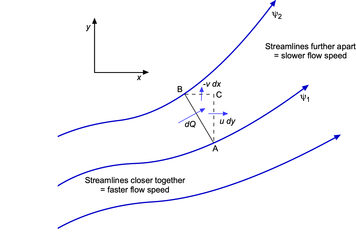
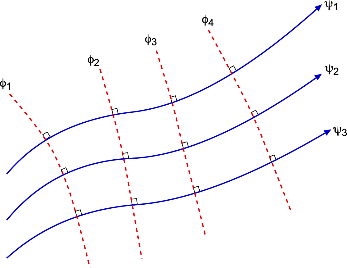
Lines of constant represent flow streamlines, and the difference in adjacent values gives the volumetric flow rate per unit depth. In other words, closer streamlines indicate higher flow velocities, as shown in the figure below. In a two-dimensional flow, the volumetric flow rate between two adjacent streamlines is given by
(26) 
Notice that there is a negative sign on the second term because, in determining the flow rate between points C and B, the integration is in the negative  direction. This result then gives
(27) 
The total differential of the stream function  is
is
(28) 
so that comparing Eqs. 27 and 28 gives
(29) 
For example, the flow rate between two adjacent streamlines,  and
and  , is
, is
(30) 
Relationship between Velocity Potential and Stream Function
In two-dimensional incompressible flow, then
(31) 
This result defines the orthogonality between streamlines ( ) and equipotential lines (
 ), as shown in the figure below.
For irrotational and incompressible flows, both and exist, and they are related through the Cauchy-Riemann equations, i.e.,
(32) 
The velocity potential and stream function are orthogonal, meaning that the gradients of and are perpendicular to each other. This geometric property is central to potential flow theory, as it implies that the flow velocity is tangent to streamlines and orthogonal to equipotential lines.
Cartesian and Polar Coordinates
The relationship between Cartesian  and polar
  coordinates is
![\[ x = r \cos \theta , \quad y = r \sin \theta , \quad r = \sqrt{x^2 + y^2} , \quad \theta = \tan^{-1}\left(\frac{y}{x}\right) \]](https://eaglepubs.erau.edu/app/uploads/quicklatex/quicklatex.com-10849fabf807c4a5f223e452b13b4ea0_l3.svg "Rendered by QuickLaTeX.com")
as shown in the figure below.
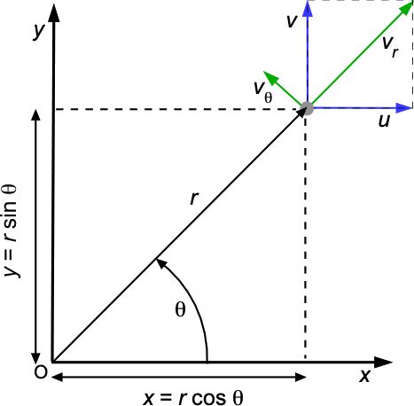 The velocity components in polar coordinates are related to the radial and angular directions. If
  are the Cartesian components of velocity, the polar components are given by
![\[ v_r = v_x \cos \theta + v_y \sin \theta, \quad \text{and} \quad v_\theta = -v_x \sin \theta + v_y \cos \theta \]](https://eaglepubs.erau.edu/app/uploads/quicklatex/quicklatex.com-a17928f114c5c8e8fd702a1a76b487e7_l3.svg "Rendered by QuickLaTeX.com")
Conversely, the Cartesian velocity components can be expressed in terms of the polar components as
![\[ v_x = v_r \cos \theta - v_\theta \sin \theta , \quad v_y = v_r \sin \theta + v_\theta \cos \theta \]](https://eaglepubs.erau.edu/app/uploads/quicklatex/quicklatex.com-5004057de8d031eb0b243e982d935321_l3.svg "Rendered by QuickLaTeX.com")
In terms of the polar components, the total velocity can be written as
![\[ \vec{V} = v_r \, \vec{e_r} + v_\theta \, \vec{e_{\theta}} \]](https://eaglepubs.erau.edu/app/uploads/quicklatex/quicklatex.com-ece7777bff0bef315f99ad78c72c5411_l3.svg "Rendered by QuickLaTeX.com")
where  and
and  are the unit vectors in the radial and angular directions, respectively.
Finally, it should be noted for reference that the Laplacian operator in polar coordinates is given by
![\[ \nabla^2 \phi = \frac{1}{r} \frac{\partial}{\partial r} \left( r \frac{\partial \phi}{\partial r} \right) + \frac{1}{r^2} \frac{\partial^2 \phi}{\partial \theta^2} \]](https://eaglepubs.erau.edu/app/uploads/quicklatex/quicklatex.com-36766a99dfc918224c64e6c150bdd545_l3.svg "Rendered by QuickLaTeX.com")
Check Your Understanding #1 – Particular solution to Laplace’s equation
Consider a steady, incompressible, irrotational flow in two dimensions where the velocity potential  satisfies Laplace’s equation, i.e.,
  The region of interest is the square
  ,
,  , with the following boundary conditions:
 on
on  ,
,  ,
,  on
on  , and
, and  on
on  .
.
- Assuming a general solution of the form
 , determine .
 - Determine the velocity field in terms of
 and
and  .
. - Verify that this velocity field is physical, incompressible, and irrotational.
- Determine the corresponding stream function for this flow.
- Sketch the streamlines and equipotential lines for this flow.
Show solution/hide solution.
1. The velocity potential satisfies Laplace’s equation, i.e.,
![\[ \nabla^2 \phi = \frac{\partial^2 \phi}{\partial x^2} + \frac{\partial^2 \phi}{\partial y^2} = 0 \]](https://eaglepubs.erau.edu/app/uploads/quicklatex/quicklatex.com-89f59545d10c097400b43bb52d4fe59a_l3.svg "Rendered by QuickLaTeX.com")
A general solution for the velocity potential of the form is to be assumed, i.e.,
![\[ \phi(x, y) = ax + by + cxy \]](https://eaglepubs.erau.edu/app/uploads/quicklatex/quicklatex.com-653cccbb96f2c13a3f77321266a11d28_l3.svg "Rendered by QuickLaTeX.com")
Substituting into Laplace’s equation, it is satisfied for any values of ,  , or
, or  . Using the given boundary conditions leads to

Therefore, the solution for the velocity potential is
![\[ \phi(x, y) = x \, y \]](https://eaglepubs.erau.edu/app/uploads/quicklatex/quicklatex.com-6133f27cef909e05b567c110b12aac86_l3.svg "Rendered by QuickLaTeX.com")
2. The velocity field is given by
![\[ u = \frac{\partial \phi}{\partial x} \quad \text{and} \quad v = \frac{\partial \phi}{\partial y} \]](https://eaglepubs.erau.edu/app/uploads/quicklatex/quicklatex.com-d9dd082f4e4c809de610e2ea86ea8608_l3.svg "Rendered by QuickLaTeX.com")
From  , then
![\[ u = \frac{\partial \phi}{\partial x} = y \quad \text{and} \quad v = \frac{\partial \phi}{\partial y} = x \]](https://eaglepubs.erau.edu/app/uploads/quicklatex/quicklatex.com-6b92e840da2409403477f5e0c6f4743a_l3.svg "Rendered by QuickLaTeX.com")
3. The vorticity  is given by
![\[ { \omega_z = \omega = \frac{\partial v}{\partial x} - \frac{\partial u}{\partial y} } \]](https://eaglepubs.erau.edu/app/uploads/quicklatex/quicklatex.com-bdd7787a8b208af9e686652f8526e5db_l3.svg "Rendered by QuickLaTeX.com")
For  and
and  , then
![\[ \frac{\partial v}{\partial x} = 1 \quad \text{and} \quad \frac{\partial u}{\partial y} = 1 \implies \omega = 1 - 1 = 0 \]](https://eaglepubs.erau.edu/app/uploads/quicklatex/quicklatex.com-1055466426df76de4405bade44018633_l3.svg "Rendered by QuickLaTeX.com")
Therefore, the velocity field is irrotational. The existence of a velocity potential means that the flow automatically satisfies continuity, i.e.,
![\[ \frac{\partial u}{\partial x} + \frac{\partial v}{\partial y} = \frac{\partial}{\partial x} \left( \frac{\partial \phi }{\partial x} \right) + \frac{\partial}{\partial y} \left( \frac{\partial \phi}{\partial y} \right) = \nabla^2 \phi = 0 \]](https://eaglepubs.erau.edu/app/uploads/quicklatex/quicklatex.com-4b699df420c6e706429250cbb377a210_l3.svg "Rendered by QuickLaTeX.com")
4. The stream function satisfies
![\[ u = \frac{\partial \psi}{\partial y} \quad \text{and} \quad v = -\frac{\partial \psi}{\partial x} \]](https://eaglepubs.erau.edu/app/uploads/quicklatex/quicklatex.com-f5811f77a893e64ba774a91252da57b4_l3.svg "Rendered by QuickLaTeX.com")
From and , then

It will be apparent, therefore, that
![\[ f(x) = -\frac{x^2}{2} \quad \text{and} \quad f(y) = \frac{y^2}{2} \]](https://eaglepubs.erau.edu/app/uploads/quicklatex/quicklatex.com-333f1b0f384ef5be7417406ef9ea2efa_l3.svg "Rendered by QuickLaTeX.com")
So, the stream function is
![\[ \psi(x, y) = \frac{y^2}{2} - \frac{x^2}{2} \]](https://eaglepubs.erau.edu/app/uploads/quicklatex/quicklatex.com-6b2de24d3e4c23249be4f2ba3dfffa86_l3.svg "Rendered by QuickLaTeX.com")
which can be confirmed by differentiation, i.e.,
![\[ u = \frac{\partial \psi}{\partial y} = y \quad \text{and} \quad v = -\frac{\partial \psi}{\partial x} = x \]](https://eaglepubs.erau.edu/app/uploads/quicklatex/quicklatex.com-84cb49487824c13573c57966c0f6fe0b_l3.svg "Rendered by QuickLaTeX.com")
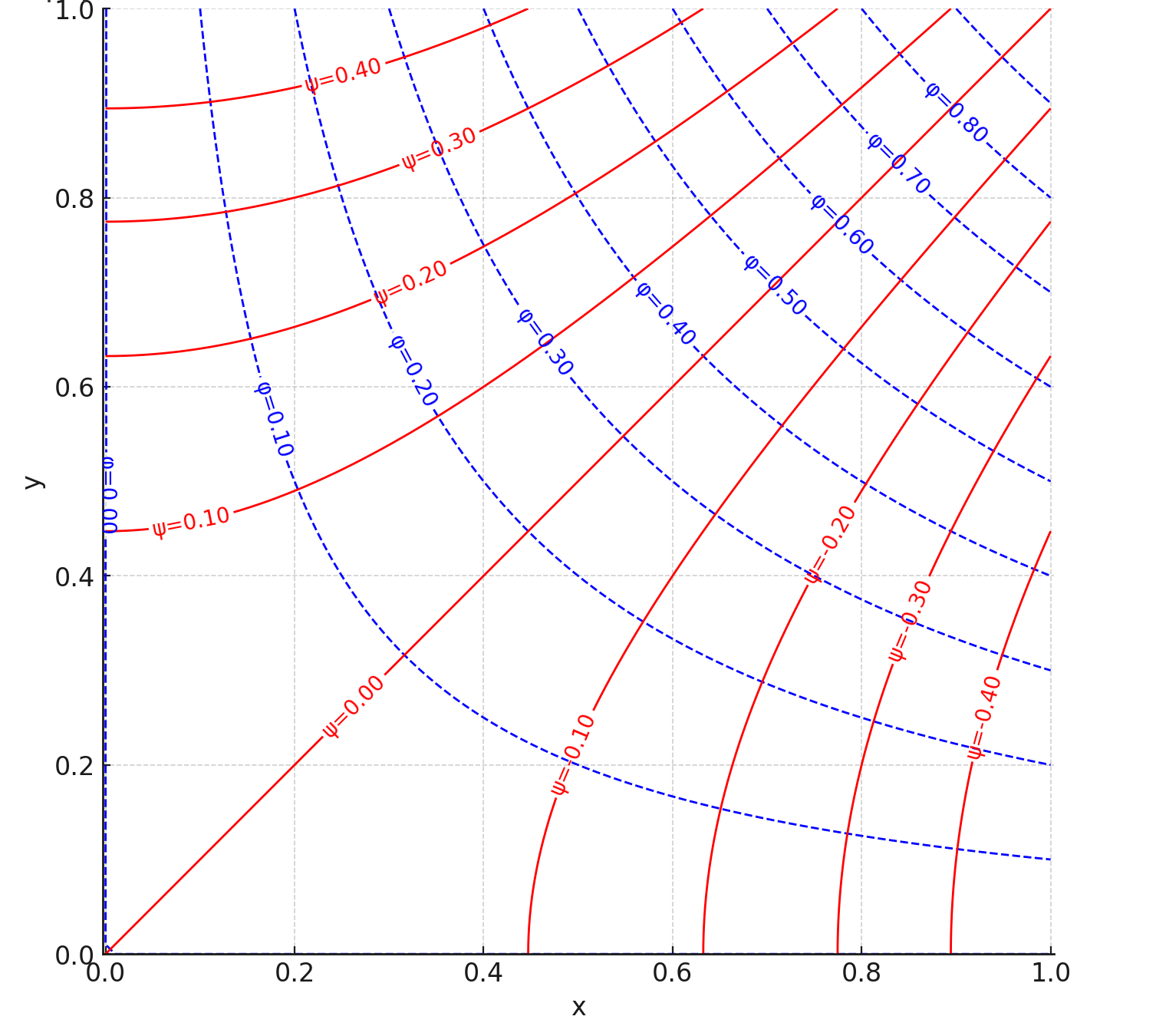
5. The streamlines correspond to constant , i.e.,
![\[ \frac{y^2}{2} - \frac{x^2}{2} = \text{constant} \]](https://eaglepubs.erau.edu/app/uploads/quicklatex/quicklatex.com-767be3fbe2c21774accf40c431c9a086_l3.svg "Rendered by QuickLaTeX.com")
The equipotential lines correspond to constant values of , i.e.,
![\[ x \, y = \text{constant} \]](https://eaglepubs.erau.edu/app/uploads/quicklatex/quicklatex.com-d1015d625743ccd01722fefe107f629d_l3.svg "Rendered by QuickLaTeX.com")
which represent orthogonal hyperbolas, as shown in the figure below.
Elementary Flows
Elementary flows are the building blocks of potential flow theory, each elementary flow satisfying Laplace’s equation. Superimposing elementary flows allows the modeling of complex flow fields. Key elementary flows include:
- Uniform flow – A constant velocity field where the flow direction and magnitude remain the same everywhere.
- Source and sink flows – Radial flow where fluid emanates from a point (source) or converges to a point (sink).
- Vortex flow – A swirling flow around a central axis characterized by circulation and rotational motion.
- Doublet flow – A combination of a source and a sink placed infinitesimally close to each other, representing the flow around slender bodies like cylinders.
Combining these elementary flows enables the analysis and visualization of more intricate flow problems, such as flow over specific classes of body shapes, including circular cylinders and ovals.
Uniform Flow
The figure below shows that a uniform flow moves at a constant velocity  in the
  direction. The equipotential lines, i.e., , are vertical lines defined by
  , and the streamlines, i.e., , are horizontal lines defined by
  , i.e.,
(33) 
 direction.
Notice that
(34) 
If the flow is moving at a constant velocity  in the
  -direction, then
(35) 
and for a flow  at an angle
  to the axis then
(36) 
These yield the correct velocity components, i.e., from the potential function, then
(37) 
and from the stream function, then
(38) 
Therefore, the velocity field is
(39) 
In polar coordinates , the potential function and stream function for a uniform flow in the direction are expressed as
(40) 
and the corresponding velocity components in polar coordinates are
(41) 
This elementary flow forms the basis for modeling freestream flows in nearly all potential-flow problems. The polar representation is beneficial for analyzing flow patterns around circular objects or in cylindrical domains.
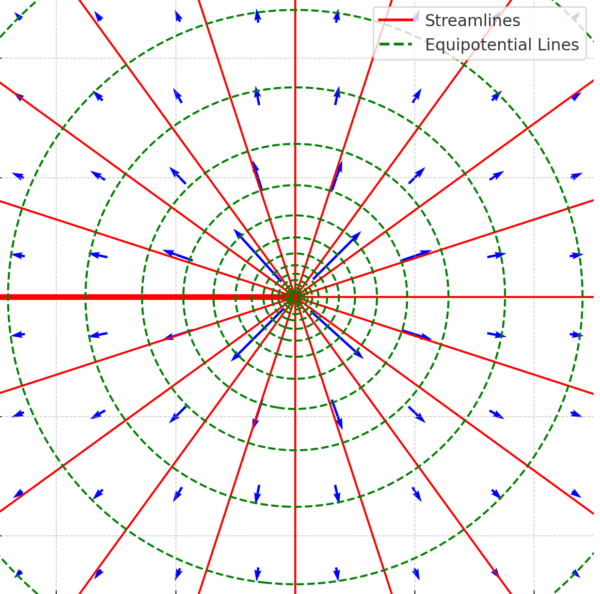
Source Flow
To derive the velocity potential and stream function for a point source, consider a steady, two-dimensional, incompressible, and irrotational flow field where fluid is emitted uniformly in all directions from a point at the origin. As shown in the figure below, a source is a hypothetical flow in which fluid “exits” from a point. The total volume flow rate per unit depth is denoted by  , which defines the source strength.
Because of the radial symmetry of the flow, the velocity vector has only a radial component  , with no tangential component
  , i.e.,
(42) 
which satisfies conservation of mass for radial outflow in two dimensions.
The velocity potential satisfies
(43) 
Substituting for and integrating with respect to  gives
gives
(44) 
The constant may be taken as zero without loss of generality, so the velocity potential becomes
(45) 
To determine the stream function , use the definitions in polar coordinates, i.e.,
(46) 
Because  , it follows that
  , so
, so  . Substituting into the expression for gives
(47) 
and integrating with respect to  gives
gives
(48) 
Again, setting the constant to zero gives the stream function as
(49) 
The final expressions for the source flow are therefore:
(50) 
where is the strength of the source, is the radial distance from the source, and is the polar angle. As shown in the figure above, the equipotential lines ( constant) are circles centered at the source, i.e., lines of constant , and are spaced in a geometric progression. The streamlines (
 constant) are straight lines radiating from the origin, i.e., lines of constant , indicating purely radial flow.
The velocity field is
(51) 
As  , the radial velocity becomes unbounded, i.e.,
  , which marks a singularity in the flow. At the origin, the assumptions of continuity and finite velocity break down. This type of behavior is characteristic of idealized elementary flows such as sources, sinks, and vortices, which are often referred to as singularities in the context of potential flow theory.
Sink Flow
A sink is the reverse of a source, where fluid is “removed” at a point, as shown in the figure below. The velocity potential and stream function are given by
(52) 
where is the (positive) strength of the sink, is the radial distance from the sink, and is the polar angle. The equipotential lines ( constant) are concentric circles centered at the origin, and the streamlines ( constant) are radial lines, as in the case of a source, but with flow directed inward.
The radial velocity is
(53) 
So the flow is purely radial and directed toward the sink at the origin. As , the velocity again becomes unbounded, indicating a singularity at the origin. Like sources, sinks are idealized representations that violate the physical assumptions of continuity at the singular point.
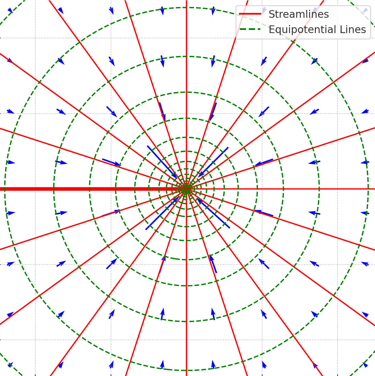
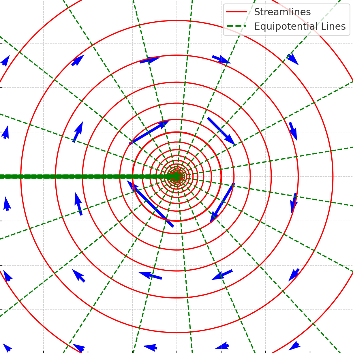
Vortex Flow (Irrotational Vortex)
A vortex flow represents purely rotational motion around the origin, as shown in the figure below, where the tangential velocity is inversely proportional to the radial distance. The equipotential lines ( = constant) are straight radial lines ( = constant), and streamlines ( = constant) are concentric circles ( = constant). The strength of the vortex is defined by the circulation  , which is the total line integral of tangential velocity around any closed loop enclosing the vortex, i.e.,
(54) 
By symmetry, the flow has no radial component, i.e.,
(55) 
where is the tangential velocity and is the radial distance from the vortex center. The direction of rotation is determined by the sign of , i.e., counterclockwise for positive , and clockwise for negative .
To derive the stream function , use the polar coordinate relations, i.e.,
(56)
Because  , it follows that
  , so
, so  . From the second equation, then
(57) 
Integrating with respect to gives
(58) 
Choosing the constant to be zero and reversing the sign (to adopt the standard convention for positive circulation yielding positive stream function), then
(59) 
To derive the velocity potential , use the relationships
(60) 
Again, implies  , so
, so  . Therefore,
(61) 
Integrating with respect to gives
(62) 
Choosing the constant to be zero and reversing the sign (again, for conventional consistency), then
(63) 
Therefore, the final expressions for the vortex flow are
(64) 
where is the circulation (a positive circulation produces a counterclockwise vortex, while a negative circulation produces a clockwise vortex), is the radial distance from the vortex center, and is the polar angle. The equipotential lines ( constant) are radial lines ( constant), and the streamlines ( constant) are circles (
 constant), indicating purely tangential flow.
The velocity field is
(65)
As , the tangential velocity becomes unbounded, i.e.,  , again indicating a singularity in the flow.
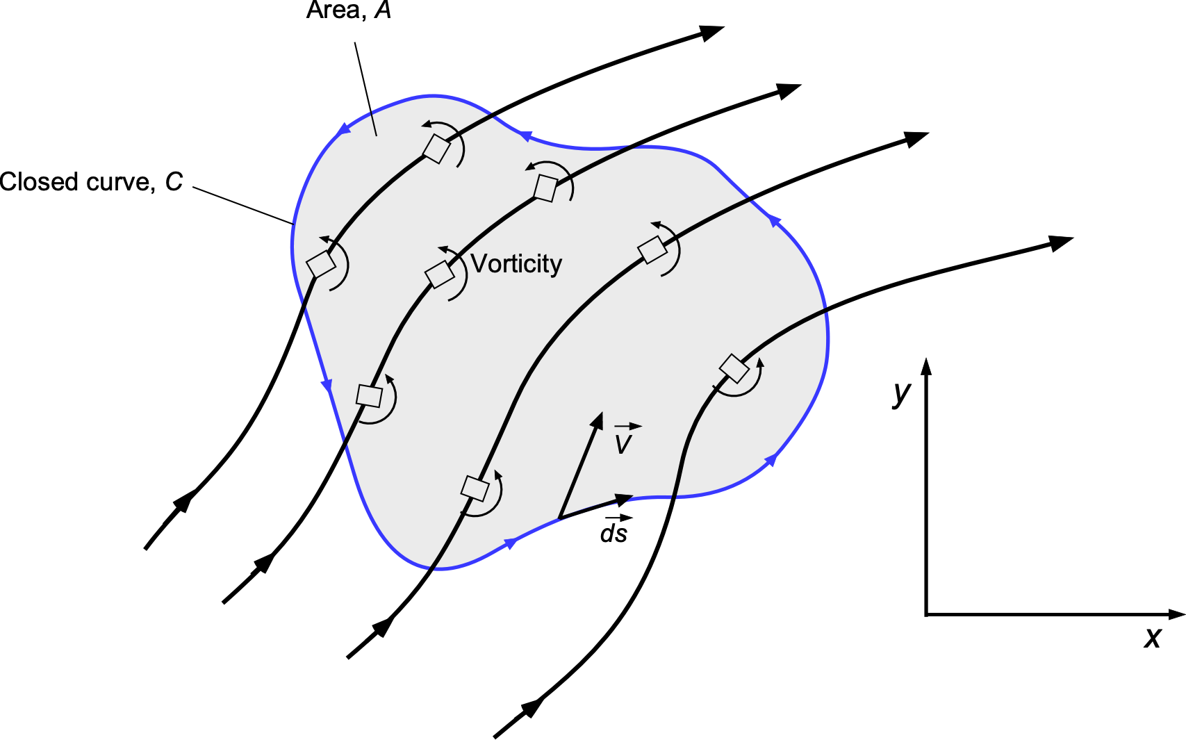
Understanding Circulation and Vorticity
The property identified as is the circulation, defined mathematically as
(66) 
where  is an infinitesimal arc length element along a closed circuit
  , and
, and  is the local velocity vector of the flow. Circulation represents the net “swirling” or “rotational” behavior of the velocity field around the circuit , as illustrated in the figure below.
-
The property of circulation is established from an integral of the velocity field around a closed path.
Circulation is calculated by integrating the velocity field along a closed path. By convention, circulation is considered positive for a counter-clockwise loop. However, the opposite convention is typically used in aerodynamics, where positive circulation corresponds to a clockwise loop, producing positive lift. If the velocity vector is expressed in components  , the circulation can also be written as
(67) 
Here, and represent the velocity components in the – and -directions, respectively. It is important to note that the presence of circulation does not necessarily imply that streamlines are circular (as in a classic vortex flow). Instead, circulation quantifies the net rotational effect of the velocity field around the chosen closed path .
Vorticity, denoted by  , is a fundamental property of a fluid flow that describes the local rotation or spinning motion of fluid elements. It is mathematically defined as the curl of the velocity field
(68) 
For two-dimensional flows in the – plane, the vorticity reduces to a scalar quantity
(69) 
where  is the out-of-plane component of the vorticity vector.
The relationship between circulation and vorticity is given by Stokes’ theorem, which connects the line integral of the velocity field around a closed curve to the surface integral of the vorticity over the enclosed area, i.e.,
(70) 
where  is the surface bounded by the closed curve ,
  is the unit normal vector to the surface, and
  is the infinitesimal area element. This relationship reveals that the circulation around a closed path is the total vorticity flux through the surface enclosed by that path. If the vorticity within the region is zero, the circulation is also zero. Notice that for potential flow, the integral of vorticity over any finite surface is zero. However, circulation can result if the path encloses a “singularity” such as a point vortex. At
  then
then  , so integrating will still give
  .
.
In summary, on the one hand, circulation provides a global measure of the rotational characteristics of the flow around a closed path. It is an integral quantity of the effect of the velocity field over a finite region. On the other hand, vorticity is a local property of the flow, describing the instantaneous rotation rate of fluid elements at each point in space. For example, in a vortex, vorticity is concentrated near its core, while circulation represents the net rotational effect when considering a closed path around the vortex. Understanding the interplay between circulation and vorticity is crucial in aerodynamics, where they play key roles in lift generation.
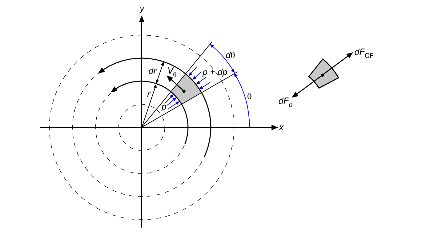
Check Your Understanding #2 – Pressure-centrifugal balance in vortex flow
Demonstrate that the existence of a steady, incompressible vortex flow requires a radial pressure gradient to balance the centrifugal forces. Use an infinitesimal control volume in the form of a fluid ring element bounded by two adjacent streamlines.
Show solution/hide solution.
Consider a steady, two-dimensional vortex flow in which the fluid moves in concentric circles about a central point. There is no radial motion, so the velocity components are
![\[ v_r = 0 \quad \text{and} \quad v_\theta = v_\theta(r) \]](https://eaglepubs.erau.edu/app/uploads/quicklatex/quicklatex.com-e129135dcf41f0bf75981b2703cefda8_l3.svg "Rendered by QuickLaTeX.com")
Examine an elemental ring of fluid bounded between radial streamlines at and  , subtending an angular width
  . The mass of the fluid element is
![\[ dm = \varrho \, dA = \varrho \, r \, dr \, d\theta \]](https://eaglepubs.erau.edu/app/uploads/quicklatex/quicklatex.com-978bf1baa9ae849accc51d7ba6ccad2b_l3.svg "Rendered by QuickLaTeX.com")
where is the fluid density.
 This element rotates about the origin with tangential velocity
  , resulting in a needed inward centripetal acceleration of
  . The corresponding outward centrifugal force is
![\[ dF_{\text{CF}} = \varrho \, v_\theta^2 \, dr \, d\theta \]](https://eaglepubs.erau.edu/app/uploads/quicklatex/quicklatex.com-bf6fec2dcc821b7f9a21e1c0ebc29f59_l3.svg "Rendered by QuickLaTeX.com")
The pressure force acts outward and inward on the inner and outer radial faces of the element, respectively. The outward pressure force at radius is
![\[ dF_{\text{out}} = p(r) \, r \, d\theta \]](https://eaglepubs.erau.edu/app/uploads/quicklatex/quicklatex.com-c617a507a5837cd8cb232d18cadd4d9a_l3.svg "Rendered by QuickLaTeX.com")
The inward pressure force at radius is
![\[ dF_{\text{in}} = p(r + dr) \, (r + dr) \, d\theta \]](https://eaglepubs.erau.edu/app/uploads/quicklatex/quicklatex.com-0093c614c99d842752dae9403ec6a04d_l3.svg "Rendered by QuickLaTeX.com")
Therefore, the net radial pressure force acting inward is
![\[ dF_p = dF_{\text{in}} - dF_{\text{out}} = p(r + dr) \, (r + dr) \, d\theta - p(r) \, r \, d\theta \]](https://eaglepubs.erau.edu/app/uploads/quicklatex/quicklatex.com-6d4c3ee55bf6714f642e8dad2d839fdd_l3.svg "Rendered by QuickLaTeX.com")
Using a Taylor series expansion of  , then
![\[ p(r + dr) = p(r) + \frac{dp}{dr} \, dr \]](https://eaglepubs.erau.edu/app/uploads/quicklatex/quicklatex.com-96ee7806b0106e3196165ee1449ee645_l3.svg "Rendered by QuickLaTeX.com")
Substituting and retaining terms to first order in  gives
gives
![\begin{align*} dF_p &= \left( p(r) + \frac{dp}{dr} \, dr \right)(r + dr) \, d\theta - p(r) \, r \, d\theta \\[8pt] &= \left( p(r) \, r + p(r) \, dr + \frac{dp}{dr} \, r \, dr \right) d\theta - p(r) \, r \, d\theta + \mathcal{O}(dr^2) \\[8pt] &= \left( p(r) \, dr + r \frac{dp}{dr} \, dr \right) d\theta + \mathcal{O}(dr^2) \end{align*}](https://eaglepubs.erau.edu/app/uploads/quicklatex/quicklatex.com-39d58af4978a9afb023cf16598b275bd_l3.svg "Rendered by QuickLaTeX.com")
Neglecting higher-order terms leads to
![\[ dF_p \approx \left( p(r) + r \frac{dp}{dr} \right) dr \, d\theta \]](https://eaglepubs.erau.edu/app/uploads/quicklatex/quicklatex.com-aafa11c3466e43e040fcd9f488bd8c4b_l3.svg "Rendered by QuickLaTeX.com")
However, only the gradient term produces a restoring force, so the net pressure force responsible for equilibrium is
![\[ dF_p \approx r \frac{dp}{dr} \, dr \, d\theta \]](https://eaglepubs.erau.edu/app/uploads/quicklatex/quicklatex.com-799914888a5b0a87ab9ad2973a323c45_l3.svg "Rendered by QuickLaTeX.com")
This radial pressure force must balance the outward-directed centrifugal force for the fluid element to remain in equilibrium. The condition for equilibrium in the radial direction is that the net radial pressure force balances the outward centrifugal force, i.e.,  , so that
![\[ r \frac{dp}{dr} \, dr \, d\theta = \varrho \, v_\theta^2 \, dr \, d\theta \]](https://eaglepubs.erau.edu/app/uploads/quicklatex/quicklatex.com-5a1e562facb4cc2864105ad18ac0a7af_l3.svg "Rendered by QuickLaTeX.com")
Canceling common factors  from both terms and rearranging gives the required pressure-centrifugal balance, i.e.,
![\[ \frac{1}{\varrho} \frac{dp}{dr} = \frac{v_\theta^2}{r} \]](https://eaglepubs.erau.edu/app/uploads/quicklatex/quicklatex.com-b7ab019e7ad438c559491bec45190384_l3.svg "Rendered by QuickLaTeX.com")
The result shows that a radial pressure gradient is required to maintain equilibrium in a steady vortex flow. Specifically, the pressure must increase with radial distance to supply the inward force that balances the outward centrifugal acceleration. This pressure gradient is a fundamental requirement for the existence of any inviscid vortex flow.
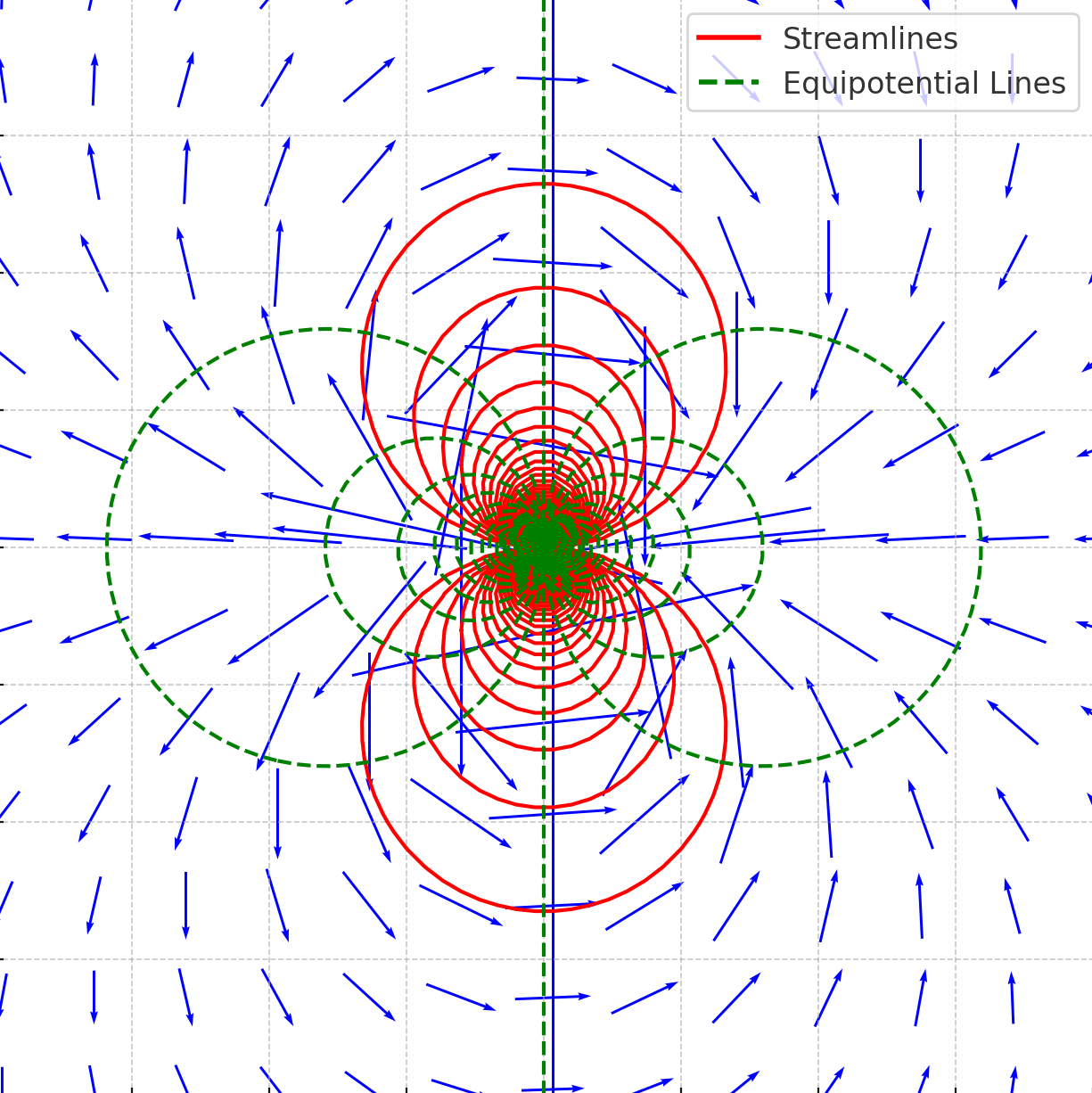
Doublet (Dipole) Flow
A doublet is created by superimposing a source and sink of equal strength placed infinitesimally close together, as shown in the figure below. A source of strength  is placed at
  , and a sink of strength
  at
at  . The separation tends to zero while maintaining a finite product of strength and separation.
The velocity potential at a point is the superposition of the potentials from the source and sink, i.e.,
(71) 
Combining logarithmic terms gives
(72) 
Now take the limit as  and
and  , such that the product
  remains finite. This limit defines a doublet of strength
  , and the velocity potential becomes
(73) 
In polar coordinates, where  and
and  , this becomes
(74) 
where  is the doublet strength. Note that a doublet has an orientation, and reversing the sign of reverses the direction of the flow.
The corresponding stream function for the doublet is
(75) 
which in polar coordinates becomes
(76) 
The velocity components in polar coordinates are obtained by differentiation of the velocity potential:
(77) 
As shown in the figure above, the streamlines of a doublet are symmetric about the -axis and form closed loops near the origin, resembling the flow around a solid body. The equipotential lines are orthogonal to the streamlines. As with other elementary flows, the doublet exhibits a singularity at the origin where the velocity becomes unbounded.
Table of Elementary Flows
A handy table of the velocity potentials and stream functions for the standard elementary flows is given below. Remember that the corresponding velocity fields are obtained using partial differentiation.
| Flow Type | Potential Function |
Streamfunction |
|---|---|---|
Uniform flow of speed at angle  |
 |
 |
 |
 |
|
| Source of strength at origin |
 |
 |
| Sink of strength at origin |
 |
 |
| Vortex of strength at origin |
 |
 |
Doublet of strength  aligned with x-axis aligned with x-axis |
 |
 |
Superposition of Elementary Flows
The linearity of Laplace’s equation allows for the principle of superposition, which states that the solution to the equation can be expressed as the sum of individual solutions. The superposition principle is a powerful tool for understanding and analyzing potential flows. It allows the construction of more intricate flow fields from simple, well-understood flow building blocks. Mathematically, this process can be written as
(78)
where  are the velocity potential functions corresponding to up to
  individual elementary flows, the values being scaling constants. More complex flow fields can be constructed to approximate or model real-world scenarios by superimposing these elementary solutions.
For example, the combination of a uniform flow and a doublet can represent the flow around a cylinder. In contrast, adding vortex and source flows can model flow around rotating bodies or specific streamline patterns. This principle is foundational in panel methods, where an airfoil or other shape is modeled as a collection of sources, sinks, and vortices distributed along its surfaces. By solving for the appropriate strengths of these elements, the flow around the airfoil can be accurately represented, including essential characteristics such as the pressure distribution and the lift.
Simulating the Flow Around a Solid Body
A solid body can replace the shape of the dividing streamline between two elementary flows, i.e., the streamline that divides one flow from another; the flow interior to the dividing streamline is irrelevant. In these cases, the value of potential methods for simulating flows around solid bodies will become increasingly apparent.
Rankine Half-Body
A Rankine half-body[4] is formed by the superposition of a uniform flow in the -direction and a source of strength located at the origin, as shown in the figure below. Rankine called such shapes “Oögenous Neoïds.”
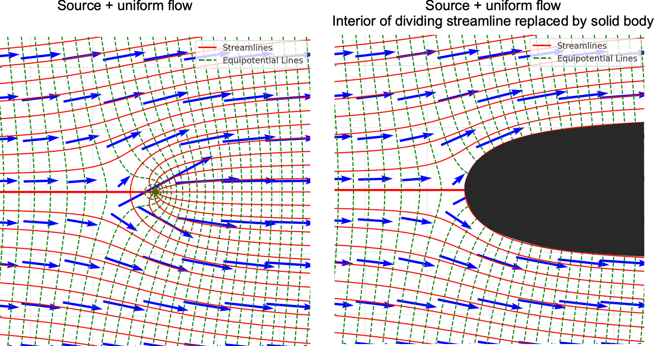
The velocity potential is
(79) 
and the corresponding stream function is
(80) 
The stagnation streamline ( ) represents the boundary of the Rankine half-body, i.e.,
(81) 
and the stagnation point ( ) occurs on the axis at
(82) 
Note that generally does not always indicate a stagnation streamline.
Rankine Oval
A Rankine oval is formed by the superposition of uniform velocity in the -direction, with a point source at  and a point sink at
  , as shown in the figure below, another Rankine neoïd. He explains, “An oval neoïd differs from an ellipse in being fuller towards the ends and flatter at the sides, and that difference is greater the more elongated the oval is.”
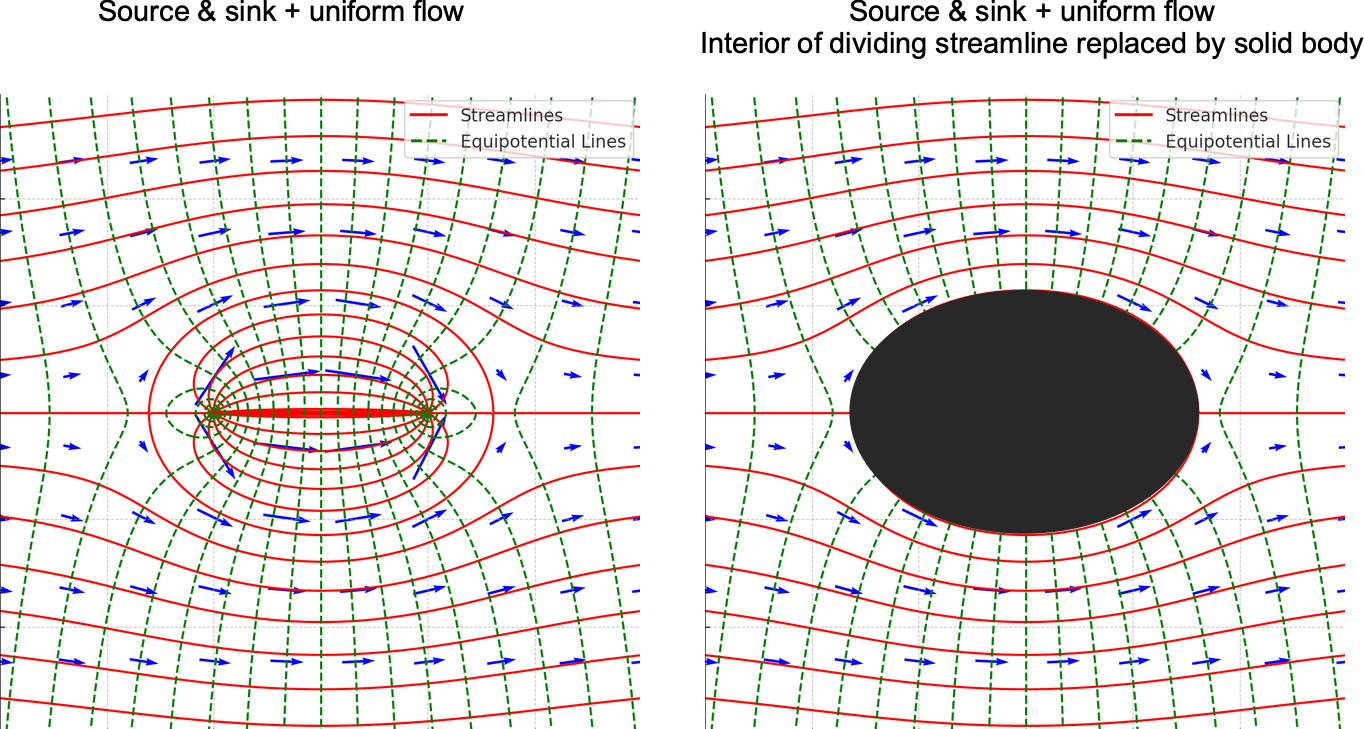
The velocity potential is
(83) 
and the stream function is
(84) 
The equation of the dividing or stagnation streamline is
(85) 
which forms the oval boundary (). Stagnation of the flow () lies on the -axis at
(86) 
provided  . Therefore, there are two stagnation points, one upstream and another downstream.
Flow Around a Circular Cylinder
The flow around a circular cylinder is a classic problem in aerodynamics. A potential flow is obtained from the superposition of the stream function from the combination of a uniform flow and a doublet, as shown in the figure below.
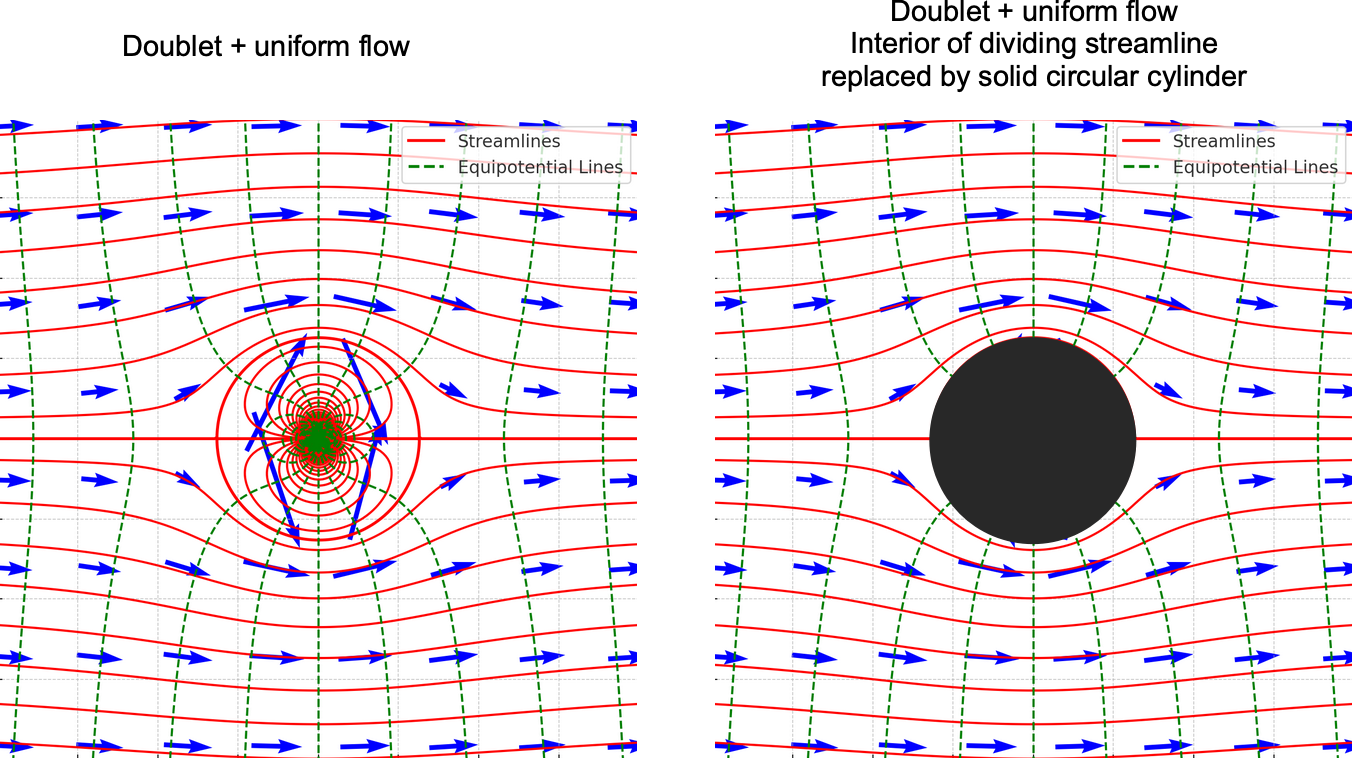
The composite stream function is given by
(87) 
For uniform flow, then
(88) 
and for a doublet at the origin, then
(89) 
The total stream function is
(90) 
Velocity on the Cylinder’s Surface
The tangential velocity is
(91) 
Taking the derivative with respect to gives
(92) 
At the surface of the cylinder ( ) and , the tangential velocity is
(93) 
Pressure on the Cylinder’s Surface
The pressure coefficient,  , is obtained using Bernoulli’s equation, i.e.,
(94) 
Therefore, the pressure coefficient at a point on the surface of the cylinder is
(95) 
Substituting the expression for  gives
gives
(96) 
This is the well-known expression for the pressure distribution around a circular cylinder in potential flow. Notice that:
- At
 and
and  (stagnation points),
  , so
, so  , indicating maximum pressure.
 - At
 and
and  (points of maximum velocity),
  , so
, so  , indicating minimum pressure.
 - The top/bottom symmetry of the cylinder will result in zero lift, and the fore/aft symmetry will result in zero drag.
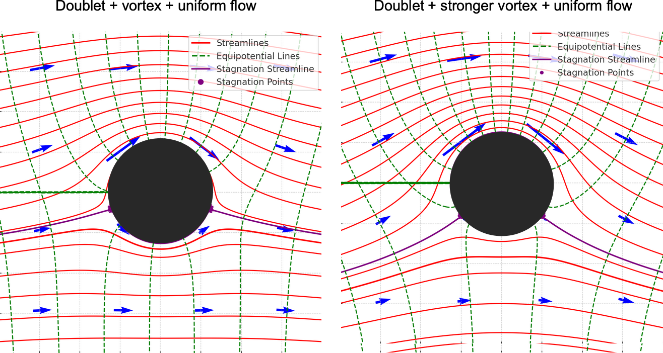
Lifting Circular Cylinder
The flow around a lifting circular cylinder is obtained by combining a uniform flow, a doublet, and a vortex, as shown in the figure below. The composite stream function is given by
(97) 
For uniform flow, then
(98)
and for a doublet at the origin, then
(99) 
Finally, for a vortex
(100) 
Therefore, the total stream function becomes
(101) 
Velocity on the Cylinder’s Surface
On the surface of the cylinder (), the velocity components are
(102) 
The stagnation points occur where  and
and  on the cylinder surface ()
(103) 
For , then
(104) 
The stagnation points are at
(105) 
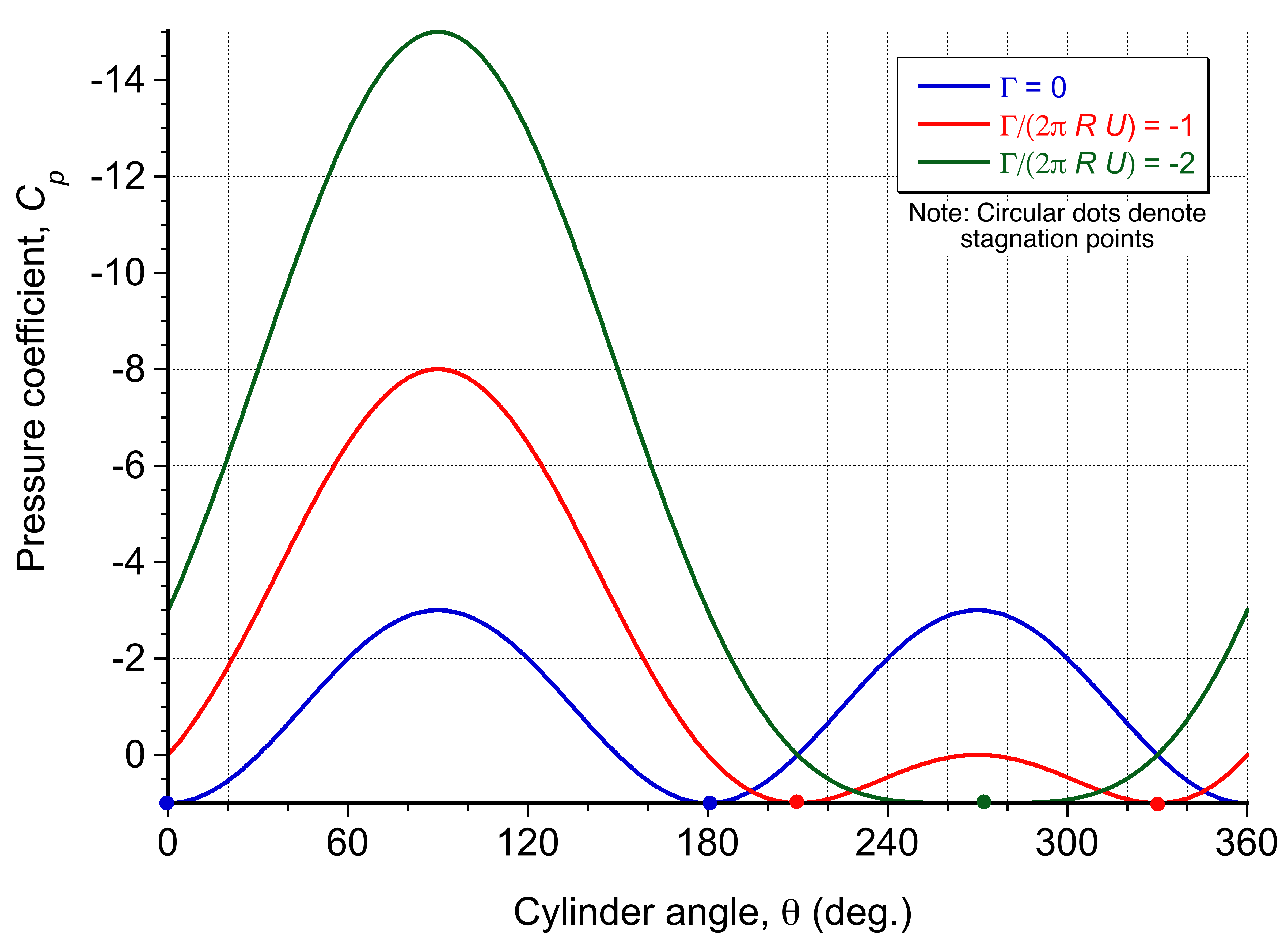
Pressure on the Cylinder’s Surface
Using Bernoulli’s equation, the pressure coefficient is given by
(106) 
where
(107) 
At the surface of the cylinder (), then
(108) 
Substituting into Eq. 106 gives
(109) 
The figure below shows representative results for two circulation values. Notice that the pressure over the upper surface becomes increasingly lower, which is responsible for generating lift. Also, note that the two initially distinct stagnation points approach each other on the lower surface and eventually merge. For increasingly higher values of circulation, known as super-circulation, the stagnation points will move away from the surface of the cylinder.
Force Components
The pressure distribution results in a force on the cylinder. Decomposing the force into – and  -directions gives
(110) 
After integration, it is found that
(111) 
because of the fore-and-aft axisymmetry of the pressure distribution, even in lifting flow. The result that the drag is zero in a potential flow is known as D’Alembert’s paradox, because drag is typically found to be finite in real flows. The reason for the “paradox” is that the flow is viscous and creates skin friction drag from the boundary layer, which eventually separates from the cylinder, generating a wake that results in significant pressure drag.
The lift force is given by
(112) 
which is called the Kutta-Joukowsky theorem, named after Martin Kutta and Nikolay Zhukovsky (or Joukowsky). This result can be interpreted from the streamlines, indicating that there is no top-bottom symmetry in this case. This latter result is very general and applies to any body shape.
The concept of circulation is inherently tied to the generation of lift, which arises from pressure differences created by the flow’s interaction with a body. Indeed, the Kutta-Joukowsky theorem’s significance extends beyond theoretical fluid dynamics to practical applications in aerodynamics. Relating lift directly to circulation provides a simple yet powerful framework for understanding and predicting the performance of airfoils, wings, and rotating objects. The theorem also explains phenomena like the Magnus lift effect on spinning balls.
Note on D’Alembert’s Paradox
D’Alembert’s paradox highlights an apparent contradiction in fluid dynamics, specifically in an ideal, non-viscous, incompressible fluid with steady, irrotational flow: a solid body (such as a cylinder) experiences no drag force. This conclusion is at odds with everyday experience, where drag is consistently observed. This historical paradox refers only to drag, but the lift is also zero. Whether this outcome is indeed a paradox depends on one’s perspective. From one viewpoint, the theoretical prediction of zero drag clashes with practical observations, making it seem paradoxical and providing fodder for mathematicians to contribute to ongoing, albeit somewhat scholarly, discussions. However, for those who understand the idealized assumptions of the potential flow model, the absence of drag aligns with the lack of mechanisms for energy dissipation, such as viscosity or turbulence, thereby rendering it a limitation of this idealized solution framework rather than a true paradox.
Method of Images
The method of solid boundary substitution, also known as the method of images, simplifies boundary condition problems in potential flows by replacing the walls and boundaries with equivalent image singularities, such as sources, sinks, and vortices. It is based on the principle of superposition and Laplace’s equation. Examples include flows near flat walls (e.g., ground effect), symmetric flows in channels or pipes, and flows around airfoils or lifting surfaces in ground effect. This method ensures uniform enforcement of boundary conditions on walls and provides solutions for linear potential flows, subject to accompanying restrictions.
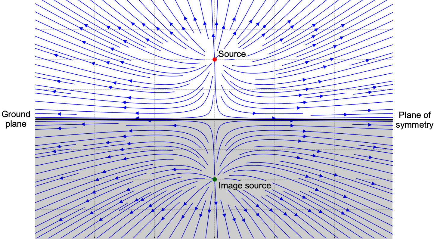
Source Flow Near a Solid Wall
Consider a point source of strength at  near an impermeable wall (
 ), as shown in the figure below. To ensure no flow normal to the wall (
 at ), place an image source of strength at
  . This ensures the cancellation of the normal velocity at . In this case he total velocity potential is
(113) 
from which the velocity field can be found using differentiation.
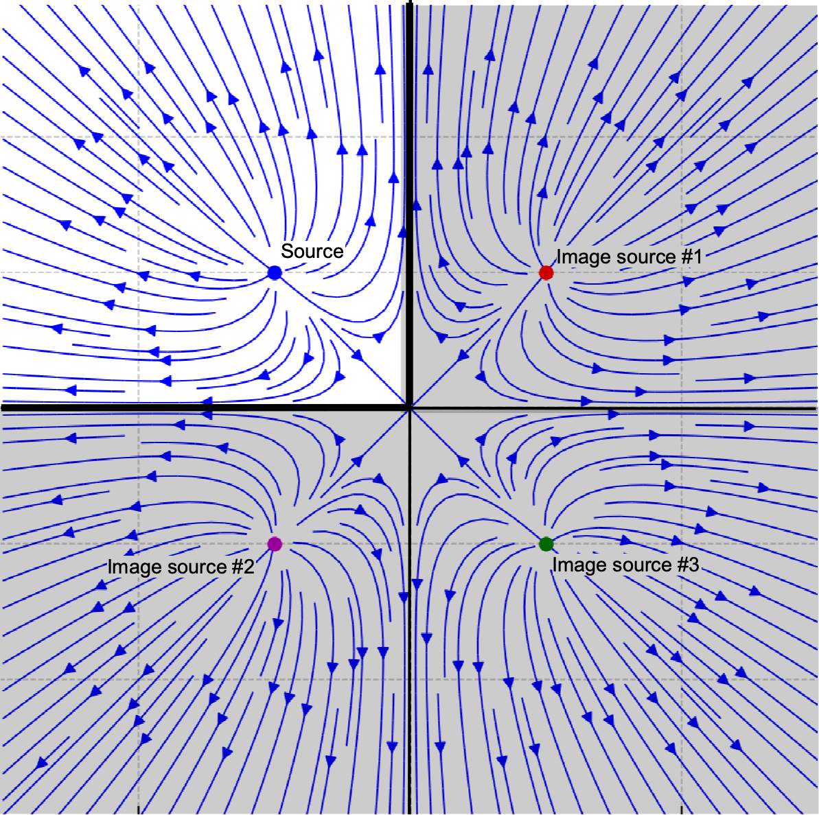
Source Flow in a Corner
Corner flow requires multiple image sources to enforce boundary conditions. For example, a corner flow problem involves placing three image sources to satisfy the conditions at both walls, as shown in the figure below. Again, the principles of superposition apply. A stationary vortex with negative circulation  is located at a height
  above a solid horizontal wall (). To satisfy the boundary condition of no flow normal to the wall (
 at ), an image vortex with positive circulation
  is placed at
  .
.
The stream function for an individual vortex in polar coordinates is given by
(114)
where is the radial distance from the vortex. The combined stream function for the real vortex and the image vortex at a point P is
(115) 
where  and
and  are given by
(116) 
Substituting  and
and  , the combined stream function becomes
(117) 
The tangential velocity induced by a vortex at a point is
(118) 
where is the distance to the vortex. The velocity component in the -direction () is
(119) 
For the real vortex
(120) 
and for the image vortex
(121) 
The total velocity in the -direction is
(122) 
At the wall where , then
(123) 
Check Your Understanding #3 – Using the method of images
above a solid horizontal wall. 1. Find an expression for the stream function for this flow and sketch the resulting streamlines. 2. Find an expression for the flow velocity induced along the wall.Show solution/hide solution.
This problem is easily solved using the method of solid boundary substitution, also known as the “method of images. The first step is to define a convenient coordinate system. In this case, there is a horizontal wall, which can be assumed to be placed along the axis. The actual or “real” vortex can then be placed at height along the axis. The axis (wall) needs to be a streamline to the flow, so the “image” vortex must be placed below the axis, as shown in the figure below. The real vortex has a negative strength or circulation, so for the image vortex, it must be ensured that it has the correct sign, i.e., for the image vortex will be positive.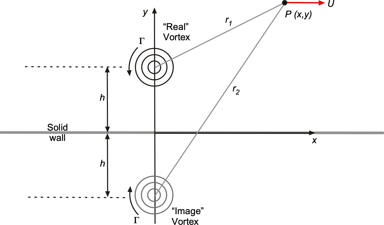
- The stream function for an individual vortex of positive strength (written in polar coordinates) is
![\[ \psi = \frac{\Gamma}{2\pi} \ln r \]](https://eaglepubs.erau.edu/app/uploads/quicklatex/quicklatex.com-2f99323f6ba0c2cb610e555484fc4255_l3.svg "Rendered by QuickLaTeX.com")
where
is the radial distance. To get the combined stream function for the real vortex and the image vortex, the radial distances of each of the vortices from the arbitrary point P must be determined. Therefore, for the combined flow![\[ \psi = \frac{(-\Gamma)}{2\pi} \ln r_1 + \frac{\Gamma}{2\pi} \ln r_2 \]](https://eaglepubs.erau.edu/app/uploads/quicklatex/quicklatex.com-084db19000d1bcc2f7da765d4fbf96a6_l3.svg "Rendered by QuickLaTeX.com")
where
and are the radial distances from the real and image vortices, respectively. The solution is incomplete because the combined flow depends on calculating these distances and in terms of and . For the real vortex, then![\[ r_1 = \sqrt{x^2 + (y-h)^2} \]](https://eaglepubs.erau.edu/app/uploads/quicklatex/quicklatex.com-823388230b9f9344f877ab353f0df377_l3.svg "Rendered by QuickLaTeX.com")
and for the image vortex, then
![\[ r_2 = \sqrt{x^2 + (y+h)^2} \]](https://eaglepubs.erau.edu/app/uploads/quicklatex/quicklatex.com-02db67a8b82f819015f424a774d5598d_l3.svg "Rendered by QuickLaTeX.com")
Using these distances and remembering the signs of the circulation on the image pair, the combined stream function for the flow is
![\[ \psi = \frac{(-\Gamma)}{2\pi} \ln \sqrt{x^2 + (y-h)^2}+ \frac{\Gamma}{2\pi} \ln \sqrt{x^2 + (y+h)^2 } \]](https://eaglepubs.erau.edu/app/uploads/quicklatex/quicklatex.com-ffca4c0e9d3d8d1992a86097969702c2_l3.svg "Rendered by QuickLaTeX.com")
or
![\[ \psi = \frac{\Gamma}{2\pi} \left( \ln \sqrt{x^2 + (y+h)^2} - \ln \sqrt{x^2 + (y-h)^2 } \right) \]](https://eaglepubs.erau.edu/app/uploads/quicklatex/quicklatex.com-c7299197cc2714171408fc8faeabb194_l3.svg "Rendered by QuickLaTeX.com")
- The velocity field can be obtained from the stream function by differentiation. Still, the velocity components can also be added in potential flows, which is usually more convenient than differentiating a stream function for which the individual elementary velocity components are already known. Remember that the tangential component
 of the induced velocity from a vortex of positive (clockwise) circulation is
![\[ V_{\theta} = -\frac{\Gamma}{2 \pi r} \]](https://eaglepubs.erau.edu/app/uploads/quicklatex/quicklatex.com-bf62f34952172ad49b402fd4385c6229_l3.svg "Rendered by QuickLaTeX.com")
where
is the distance to the arbitrary point P. Notice that a potential vortex does not induce a  component. The component can be resolved in any direction. In the direction, i.e., parallel to the wall, the
  part is used so that
![\[ u = -\frac{\Gamma}{2 \pi r} \sin \theta \]](https://eaglepubs.erau.edu/app/uploads/quicklatex/quicklatex.com-81a881f8115edc973c81b2a0f7296560_l3.svg "Rendered by QuickLaTeX.com")
For a Cartesian to polar conversion
 , so that
![\[ u = -\frac{\Gamma}{2 \pi r} \left( \frac{y}{r} \right) = -\frac{\Gamma y}{2 \pi r^2} \]](https://eaglepubs.erau.edu/app/uploads/quicklatex/quicklatex.com-84696af74c504a00e26ab1e7918883fd_l3.svg "Rendered by QuickLaTeX.com")
Therefore, for our problem (and continuing to remember the signs on the vortices and their relative offsets from the
axis), then![\[ U = \frac{-(-\Gamma) (y-h)}{2 \pi (x^2+(y-h)^2)} + \frac{\Gamma (y+h)}{2 \pi (x^2+(y+h)^2)} \]](https://eaglepubs.erau.edu/app/uploads/quicklatex/quicklatex.com-14b5d02bbede2f3cb32133576fa0fb5b_l3.svg "Rendered by QuickLaTeX.com")
or
![\[ U = \frac{\Gamma}{2 \pi} \left( \frac{(y+h)}{x^2+(y+h)^2} + \frac{(y-h)}{x^2+(y-h)^2} \right) \]](https://eaglepubs.erau.edu/app/uploads/quicklatex/quicklatex.com-3a90974c290b090faa3a58a2416ab9df_l3.svg "Rendered by QuickLaTeX.com")
By setting
= 0 (i.e., on the wall), the flow velocity can be determined there, which is![\[ U = \frac{\Gamma}{2 \pi} \left(\frac{h}{(x^2+h^2)} + \frac{h}{(x^2+h^2} \right) = \frac{\Gamma}{\pi} \left(\frac{h}{x^2+h^2} \right) \]](https://eaglepubs.erau.edu/app/uploads/quicklatex/quicklatex.com-0d7555d1d73b84b8a145a2712143c967_l3.svg "Rendered by QuickLaTeX.com")
This result clearly shows that the peak velocity on the wall is directly below the vortex and drops quickly on either side as one moves along the wall.
Three-Dimensional Potential Flow Around a Sphere
A uniform flow in the -direction has the velocity potential
(124) 
where is the freestream velocity, and  in axisymmetric spherical coordinates.
The velocity potential of a doublet aligned along the -axis in spherical coordinates is
(125) 
where is the doublet strength,  is the radial distance, and
  , noting that the flow is axisymmetric about the -axis.
The total velocity potential is the sum of the uniform flow and doublet potentials, i.e.,
(126) 
In spherical coordinates, substituting gives
(127) 
The velocity components coordinates are obtained by taking derivatives of  , i.e.,
(128) 
and
(129) 
because the flow is axisymmetric about the -axis.
The flow tangency (no-penetration) condition at the sphere’s surface at ensures that  at .
at .
This latter result is automatically satisfied because
(130) 
The corresponding tangential component is
(131) 
which for gives
(132) 
Therefore, the pressure coefficient on the surface of the sphere is
(133) 
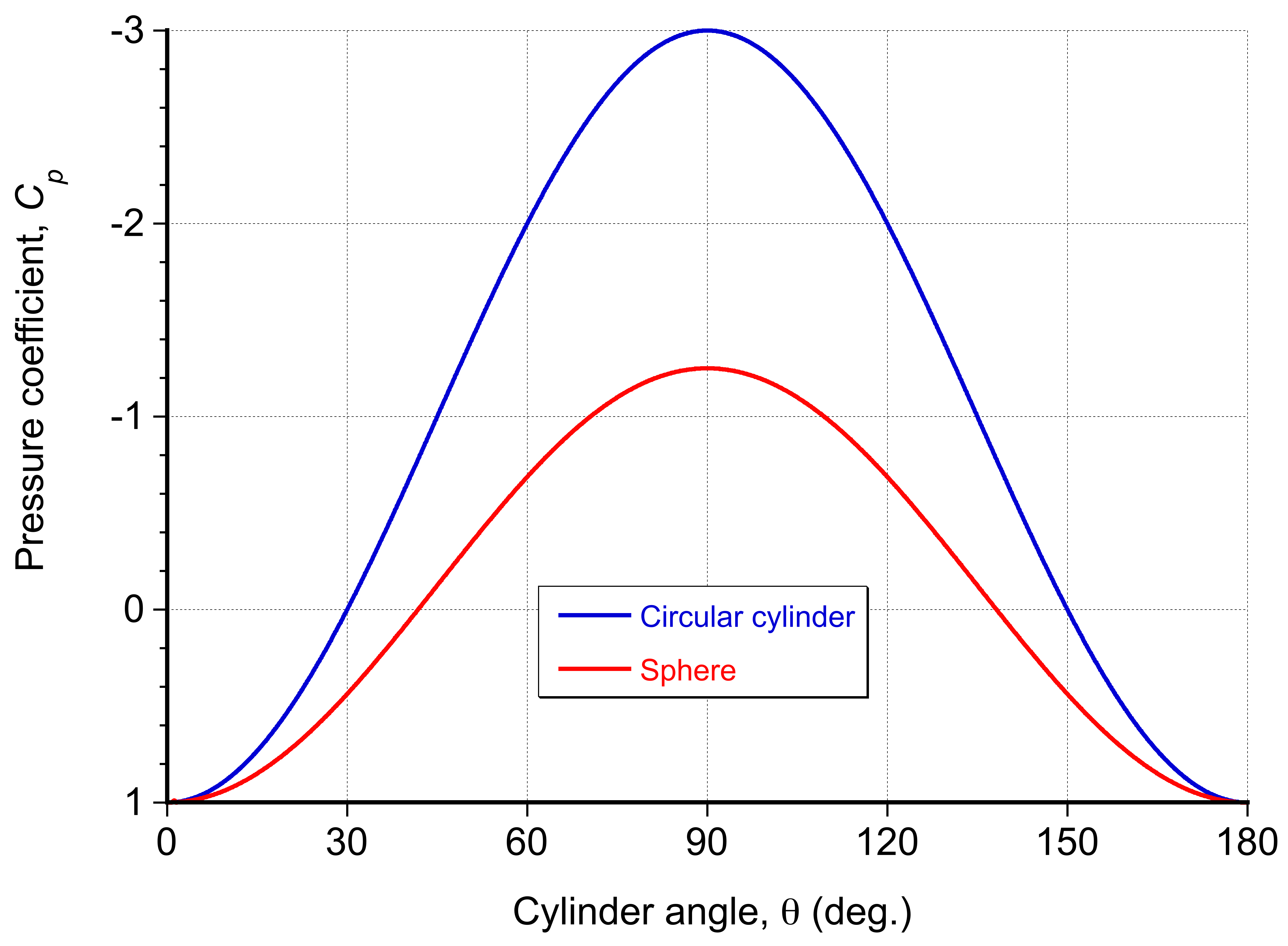
The flow around a sphere exhibits spherical axisymmetry, meaning the flow field remains invariant about the -axis. The maximum velocity occurs at the sphere’s equator ( =  ), is 1.5 , with a minimum pressure coefficient of
  . In contrast, the flow around a cylinder is two-dimensional, being symmetric only in the plane perpendicular to its axis, with a maximum velocity of
  and a minimum pressure coefficient of
  . This difference arises from the three-dimensional “relieving effect” in that, in addition to moving over and under the sphere, the flow can also move spanwise. As shown in the figure below, this extra “freedom” in the motion of the flow reduces the velocity and pressure gradients on the sphere compared to the cylinder.
Complex Variable Methods in Potential Flow
Complex variable theory provides a powerful yet elegant framework for solving two-dimensional potential flow problems. A key idea is that instead of working with separate – and -coordinates, these can be combined into a single complex number, i.e.,
(134) 
where  is the imaginary unit. Notice that
(135) 
This formulation enables both the geometry and the flow to be described using functions of a single complex variable. Notice also that
(136) 
In potential flow theory, the flow is represented by a complex potential function given by
(137) 
where is the velocity potential and is the stream function. These two quantities describe the fluid motion: streamlines are contours of constant , and equipotential lines are contours of constant .
The complex function  is assumed to be analytic, meaning it has a well-defined complex derivative with respect to
  . The condition for analyticity is that the real and imaginary parts of , namely and , satisfy the Cauchy-Riemann equations given previously in Eq. 32. Satisfying these equations ensures that the flow is both irrotational and incompressible. The gradient of gives the velocity vector, and the stream function is orthogonal to it at every point. Hence, the streamlines and equipotential lines are always perpendicular, a fundamental property of potential flows that has already been explained.
Velocity Field
The velocity vector is  , so differentiating the complex potential with respect to gives
(138) 
Using the chain rule, then
(139) 
Because and satisfy the Cauchy-Riemann conditions, where
(140) 
then  , and it follows that
(141) 
which is the complex conjugate of the velocity vector. This expression is central to complex potential theory, as it allows the velocity field to be obtained directly from the derivative of the complex potential.
Satisfying Laplace’s Equation
Because  is analytic, differentiate the first equation with respect to to obtain
(142) 
and differentiate the second equation with respect to to obtain
(143) 
Adding the two latter results gives
(144) 
because mixed partials are equal. Therefore,
(145) 
which is Laplace’s equation. A similar argument shows that is harmonic, i.e.,
(146) 
These results confirm that complex potential theory is fully consistent with the requirements of two-dimensional potential flow.
Because both the and functions satisfy Laplace’s equation, their combination into a single function inherits the powerful tools of complex analysis, i.e.,
(147) 
which is the principle of superposition because
(148) 
This complex variable framework simplifies the construction and manipulation of potential flow solutions. Simple flow patterns, such as uniform flow, point sources and sinks, doublets (dipoles), and vortices, can now be represented by a corresponding complex velocity potential. These building blocks can be combined through superposition to form more complex flows, as already explained earlier in this chapter.
Another significant advantage of the complex variable approach is that it provides a direct method to compute forces and moments acting on bodies from the flow field. These concepts form the theoretical foundation of classical airfoil theory, illustrating the intrinsic relationship between circulation and lift using the Blasius theorem. While the use of complex variables may initially feel unfamiliar to many students, the structure they provide leads to significant analytical clarity and efficiency.
Working with Complex Potentials
The use of complex potentials in potential flow theory is best understood by examining a few examples. Consider a uniform flow of speed in the -direction. The complex potential for this flow is
(149) 
and the complex velocity is
(150) 
which is constant and purely real. Now, introduce a point source of strength at the origin. Its complex potential is
(151) 
and the corresponding velocity is
(152) 
These two flows can be superimposed to give
(153) 
The resulting flow describes uniform flow disturbed by a point source, known as a Rankine half-body, which has previously been examined in some detail. The flow field can be visualized as discussed previously by examining the streamlines, which correspond to lines of constant .
Table of Complex Potentials for Elementary Flows
A handy table of the complex potentials for the complete set of standard elementary flows is given below.
| Flow Type | Complex Potential |
Velocity  |
|---|---|---|
| Uniform flow at angle to the -axis |
 |
 |
| Source of strength at the origin |
 |
 |
| Sink of strength at the origin |
 |
 |
| Vortex of strength at the origin |
 |
 |
| Doublet of strength at the origin |
 |
 |
Check Your Understanding #4 – Complex potential for a circular cyclinder in a uniform flow
Construct the complex potential for two-dimensional potential flow around a stationary circular cylinder of radius  , centered at the origin, placed in a uniform stream of velocity directed along the -axis. Identify the location of the stagnation points and verify that the surface of the cylinder corresponds to a streamline. Derive an expression for the stream function in polar coordinates and confirm that the streamline corresponds to the cylinder boundary.
Show solution/hide solution.
The flow can be modeled as a superposition of a uniform flow and a doublet located at the origin. A uniform flow of speed in the -direction has the complex potential
![\[ w_{\text{uniform}}(z) = Uz \]](https://eaglepubs.erau.edu/app/uploads/quicklatex/quicklatex.com-1248100312a88ffb02a200ae57a28125_l3.svg "Rendered by QuickLaTeX.com")
A doublet of strength at the origin has the complex potential
![\[ w_{\text{doublet}}(z) = \frac{\kappa}{2\pi z} \]](https://eaglepubs.erau.edu/app/uploads/quicklatex/quicklatex.com-e97c54ff7bad705ace2bc58ff99176f8_l3.svg "Rendered by QuickLaTeX.com")
By linear superposition, the total complex potential is
![\[ w(z) = Uz + \frac{\kappa}{2\pi z} \]](https://eaglepubs.erau.edu/app/uploads/quicklatex/quicklatex.com-0820db43695d9c02b6aecf33ed200439_l3.svg "Rendered by QuickLaTeX.com")
To determine the appropriate doublet strength , consider the location of stagnation points, where the complex velocity vanishes, i.e.,
![\[ \frac{dw}{dz} = U - \frac{\kappa}{2\pi z^2} \]](https://eaglepubs.erau.edu/app/uploads/quicklatex/quicklatex.com-587948e9cb31d0ce57de137c99210b23_l3.svg "Rendered by QuickLaTeX.com")
Setting  gives
gives
![\[ z^2 = \frac{\kappa}{2\pi U} \quad \text{so that} \quad z = \pm \sqrt{\frac{\kappa}{2\pi U}} \]](https://eaglepubs.erau.edu/app/uploads/quicklatex/quicklatex.com-9dfbb6a76caddc8956c1aedd83d00ee1_l3.svg "Rendered by QuickLaTeX.com")
These stagnation points define the outermost streamline enclosing the cylinder. Define the cylinder radius as
![\[ R = \sqrt{\frac{\kappa}{2\pi U}} \quad \text{so that} \quad \kappa = 2\pi U R^2 \]](https://eaglepubs.erau.edu/app/uploads/quicklatex/quicklatex.com-380dd741830438323735af69c3ad2f0d_l3.svg "Rendered by QuickLaTeX.com")
Substituting this into the complex potential gives the final expression
![\[ w(z) = Uz + \frac{UR^2}{z} \]](https://eaglepubs.erau.edu/app/uploads/quicklatex/quicklatex.com-4beac5608d24b7604613b893944fc669_l3.svg "Rendered by QuickLaTeX.com")
The complex velocity field is obtained by differentiation, i.e.,
![\[ V(z) = \frac{dw}{dz} = U - \frac{UR^2}{z^2} \]](https://eaglepubs.erau.edu/app/uploads/quicklatex/quicklatex.com-db1b0192c8303e7877e43cdd34a885fe_l3.svg "Rendered by QuickLaTeX.com")
Setting  = 0 again confirms the stagnation points at
  , which lie on the surface of the cylinder.
To find the streamlines, use polar coordinates  so that
![\[ w(z) = U\left( re^{i\theta} + \frac{R^2}{r}e^{-i\theta} \right) \]](https://eaglepubs.erau.edu/app/uploads/quicklatex/quicklatex.com-151c6e55e440496f55fa850027228ffd_l3.svg "Rendered by QuickLaTeX.com")
Taking the imaginary part gives the stream function as
![\[ \psi = U\left( r \sin\theta - \frac{R^2}{r} \sin\theta \right) = U \sin\theta \left( r - \frac{R^2}{r} \right) \]](https://eaglepubs.erau.edu/app/uploads/quicklatex/quicklatex.com-789bc2086e1f3aacd32366075fed0783_l3.svg "Rendered by QuickLaTeX.com")
The streamline defined by = 0 occurs either when  , which corresponds to the axis of symmetry, or when , which defines the surface of the cylinder. This result confirms that the cylinder surface coincides with a streamline and that the potential flow model satisfies the flow-tangency boundary condition.
Conformal Transformations
Before studying conformal transformations, it is advisable to revise the principles of complex mathematics. Within the framework of two-dimensional potential flows in terms of complex variables, conformal transformations (or mappings), utilize complex analytic functions that preserve angles locally,[5] enabling the transfer of closed-form solutions for canonical-shaped boundaries, while rigorously satisfying Laplace’s equation and the non-penetration boundary condition. The mathematical foundations of conformal transformations were laid down in the nineteenth century by Carl Gauss and further developed by William Thomson (Lord Kelvin), who applied these transformation techniques to generate new potential flows from known ones. Bernhard Riemann subsequently completed the theoretical framework that underpins the modern aerodynamic applications of conformal transformations.
A conformal mapping is an analytic transformation, say  , which transforms each point given by
  in one complex plane to new points
  in another plane, while preserving the local angle between intersecting functions and curves. Consequently, streamlines and equipotential lines, which are orthogonal in a potential flow field, remain orthogonal after the transformation, although their shapes will generally deform, as shown in the figure below.
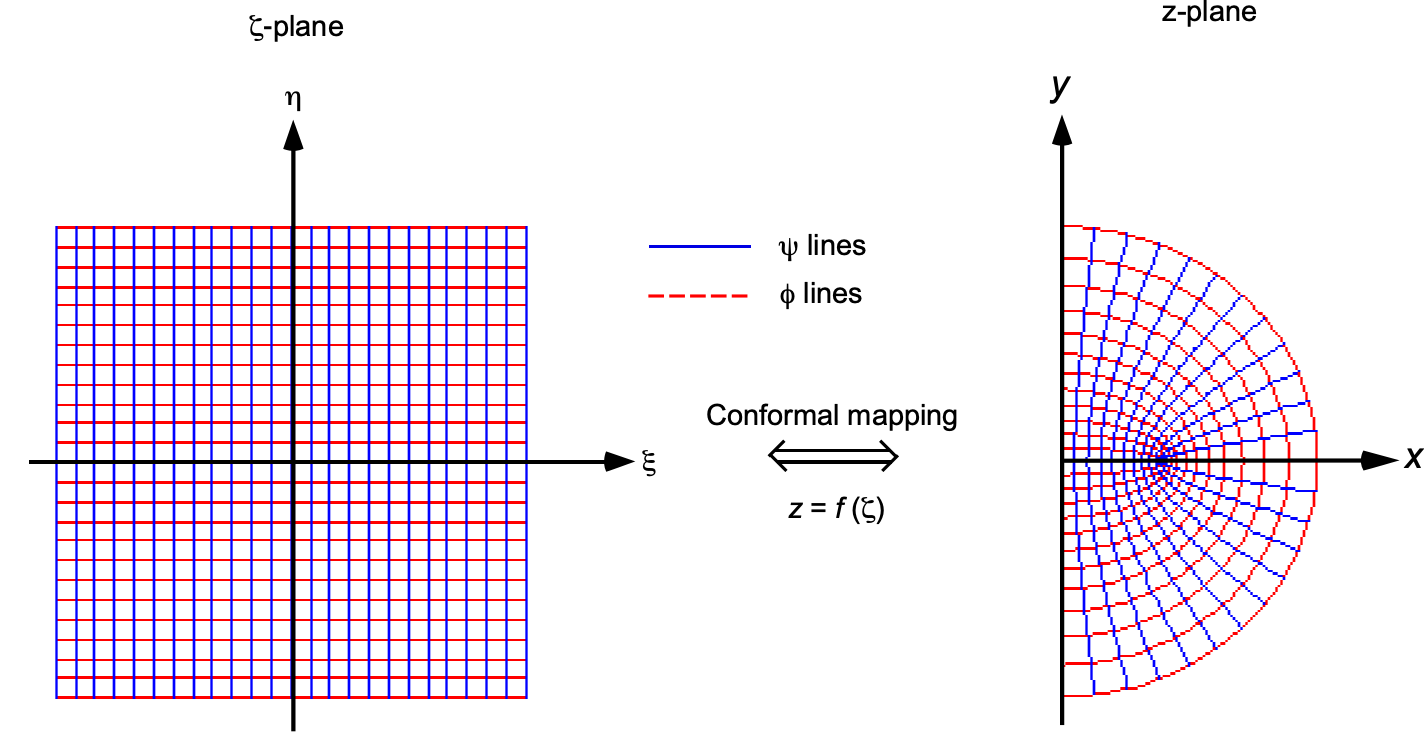
Because conformal mappings preserve harmonicity, any velocity potential or stream function satisfying Laplace’s equation in the  -plane also satisfies it in the -plane. This property allows the construction of an aerodynamic flow solution in two steps: first, solve the potential flow around a known geometry in the -plane; second, apply an appropriate conformal transformation
  to map that solution onto a boundary in the -plane, thereby obtaining the new potential flow field.
The complex potential in the -plane is given by
(154) 
where
(155) 
After mapping , the complex potential in the physical plane becomes
(156) 
with  . The velocity components then follow from
(157) 
Because  is analytic in the -plane, its real and imaginary parts satisfy the Cauchy–Riemann relations, i.e.,
(158) 
so that both and are harmonic and satisfy the Laplace equation, i.e.,
(159) 
Basic Conformal Transformations in Aerodynamics
In two-dimensional potential flow theory, conformal transformations are used to map simple geometric domains, such as circles, into more complex shapes, like airfoils. These transformations preserve angles locally and ensure that the governing Laplace equation remains valid under the mapping. Several elementary conformal transformations form the foundation for constructing more complex aerodynamic mappings. The most important of these are translation, rotation, scaling, and inversion.
A translation moves every point in the flow field by a fixed vector
(160) 
where  is a complex constant. This operation shifts the geometry and the entire flow field without altering its structure or properties. A rotation about the origin is given by
(161) 
which rotates the geometry counterclockwise by an angle . This transformation preserves distances and angles and is commonly used to orient flow fields. Uniform stretching or shrinking of the domain is achieved by
(162) 
This transformation scales all lengths by a factor , modifying the size of the flow domain while preserving shape. The velocity field scales inversely with , affecting the dynamic pressure. Combined rotation and scaling can be combined into a single transformation, i.e.,
(163) 
which simultaneously rotates and stretches the geometry. An inversion transforms points near the origin to far away and vice versa, i.e.,
(164) 
This is a nonlinear transformation that reverses orientation and is singular at  . It plays a key role in more advanced mappings such as the Joukowsky transformation. All of these transformations are summarized in the figure below.
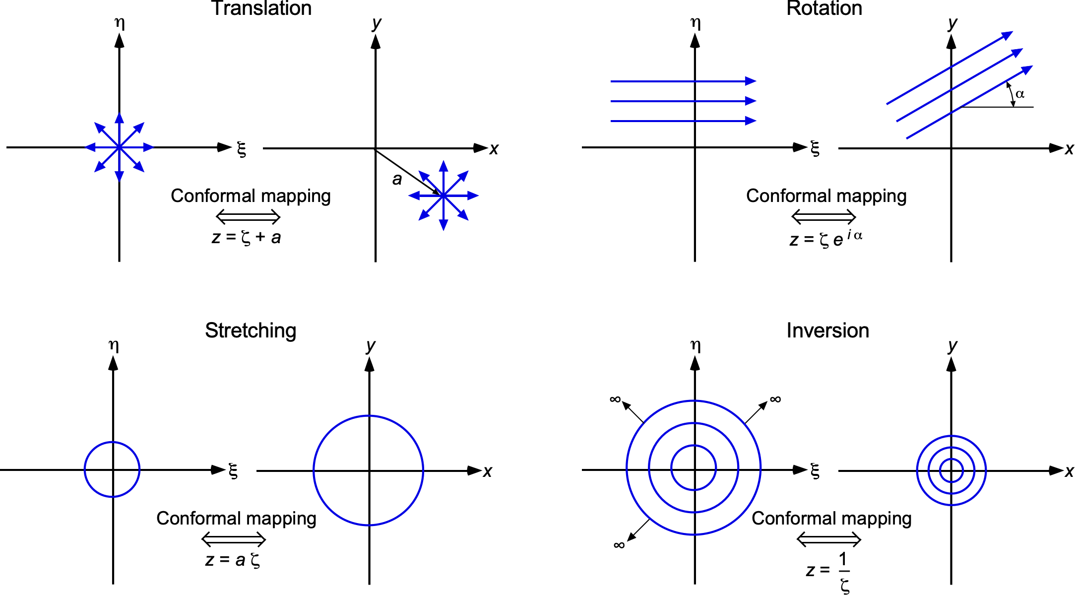
Finally, the most general linear-fractional conformal mapping is
(165) 
where  ,
,  ,
,  and
and  are any complex numbers. This is a class of transformations called Möbius transformations, which includes translation, rotation, scaling, and inversion as special cases. Möbius transformations are especially useful in constructing mappings between circular domains or for handling complex boundary conditions. These basic transformations can be composed to generate more elaborate transformations, such as the Joukowsky map. While the underlying mathematics can become intricate, many useful aerodynamic mappings rely only on simple combinations of these fundamental operations.
Flow in a Corner
Consider an example of a conformal transformation of a uniform flow using the mapping  . Under a conformal transformation, every analytic solution of Laplace’s equation in the -plane can be carried over to the -plane simply by substituting
  . The flow in a right-angled corner is obtained when
  , which is used as a special case.
In the computational (or “”) plane, there is a uniform flow of velocity in the positive  direction. In that plane
(166) 
so that
(167) 
Notice that the equipotential lines  are vertical lines
  , and the streamlines
  are horizontal lines
  .
.
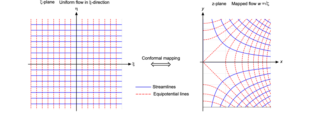
 = 2, i.e.,
  . Notice that the conformal mapping maintains the orthogonal relationship between the streamlines and equipotential lines.
Mapping into the physical (or “”) plane using  gives
gives
(168) 
so that
(169) 
Notice that equipotential lines now become parabolas defined by  , while streamlines become hyperbolae with
  ; angle preservation ensures they remain orthogonal after the mapping.
In general, substituting (or ) transforms a uniform flow in the -plane into flow in a wedge in the -plane. To see this, let the complex potential in the -plane be
(170) 
so that
(171) 
The streamlines and equipotential lines are therefore spaced radially in a pattern that repeats every  radians. This means the flow in the -plane occupies a wedge of angle .
Different values of in the transformation produce flows in different wedge geometries. If  , then the wedge in the
  -plane has an opening angle of
  , corresponding to a sector of one-third of a full circle. Conversely, if
  , then the mapping corresponds to a wedge of
  , which folds the flow multiple times around the origin. A value of
  gives a wedge angle of
  , which can model flow into a wide concave corner. This flexibility enables conformal mappings to be tailored to various practical geometries, including those with both convex and concave wedge boundaries.
Transformation of a Circular Cylinder to an Airfoil
This specific conformal transformation is named after Nikolai Zhukovsky (Joukowsky), who generalised the conformal mapping technique[6] to convert a suitably placed circle into an airfoil profile with a cusped trailing edge, now known as the classic Joukowsky airfoil.
In the -plane, start with a circular cylinder of radius centered at
(172) 
Typically, = 1. The points on the circle are
(173) 
Recall that a conformal transformation maps points in the ( ) plane to the (
 ) plane. In this case, the Joukowsky conformal mapping into the -plane is
(174) 
and substituting  gives
gives
(175) 
Separating the real and imaginary parts gives
(176) ![\begin{equation*} \begin{aligned} x(\theta) &= \xi_0 + a\cos\theta + \frac{a^2\,\bigl(\xi_0 + a\cos\theta\bigr)}{\xi_0^2 + 2a\,\xi_0\cos\theta + a^2}\\[8pt] y(\theta) &= \eta_0 + a\sin\theta - \frac{a^2\,\bigl(\eta_0 + a\sin\theta\bigr)}{\xi_0^2 + 2a\,\xi_0\cos\theta + a^2} \end{aligned} \end{equation*}](https://eaglepubs.erau.edu/app/uploads/quicklatex/quicklatex.com-d995296b1533e1bab34a68f673c0252b_l3.svg "Rendered by QuickLaTeX.com")
For a non-lifting flow ( ) about the cylinder, the complex potential in the -plane is
(177) 
Under , the same  describes the flow in the -plane, i.e.,
(178) 
For a zero offset = 0 with  = 0 and
  = 0, the transformation produces a flat plate with zero thickness. Because the circle is described by
  , where
  , then under the transformation
(179) 
which is real and represents a horizontal flat line in the plane. Notice that the chord of the flat plate, , and for the Joukowsky airfoils in general, is 4, i.e., = 4 after the transformation from the -plane to the -plane.
However, by choosing the offset  with
with  , the camber and trailing‐edge shape of the resulting Joukowsky airfoil can be controlled, all while preserving the analytic potential flow solution using a single substitution. As shown in the figure below, a -offset introduces thickness into the mapped airfoil profile without altering its symmetrical shape about the chord line.
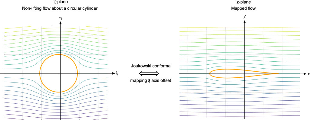
 along the -axis.
A combined -axis and  -axis offset, i.e.,
  , skews the airfoil contour and streamlines, creating both camber and thickness asymmetry, as shown in the figure below. The stagnation points shift chordwise and/or vertically, demonstrating the complete control of the airfoil shape and its flow that results from displacements of the cylinder center in the -plane.
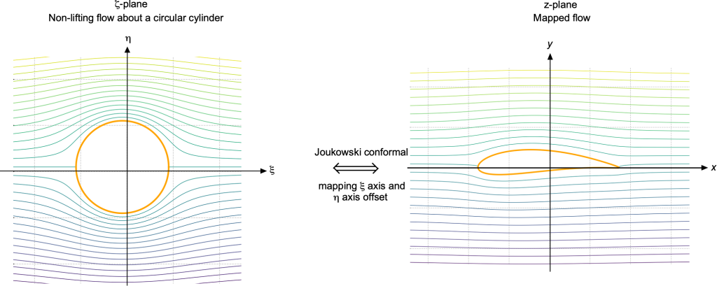
 along the and axes.
The local complex velocity on the airfoil surface is
(180) 
Therefore, the tangential velocity is
(181) 
and the pressure coefficient follows as
(182) 
The figure below shows the nominally non-lifting pressure coefficient distribution versus chordwise position  for the upper and lower surfaces of a Joukowsky airfoil with offsets = -0.1, = 0.05, and = 1. A slight leading-edge suction with a negative peak is on the lower surface immediately downstream of the leading edge. Moving aft, the suction gradually weakens (with rising toward zero) along the upper surface, whereas the upper surface experiences milder suction and remains closer to ambient pressure. At the trailing edge, both curves approach = 0 at = 1, reflecting the zero net pressure jump at the end of the cusp. This separation of upper and lower surfaces clarifies how thickness (from the offset) and camber/asymmetry (from the offset) produce a non-uniform pressure distribution over the surface even with no net lift (i.e., zero net circulation). The lifting cases are considered in the next chapter.
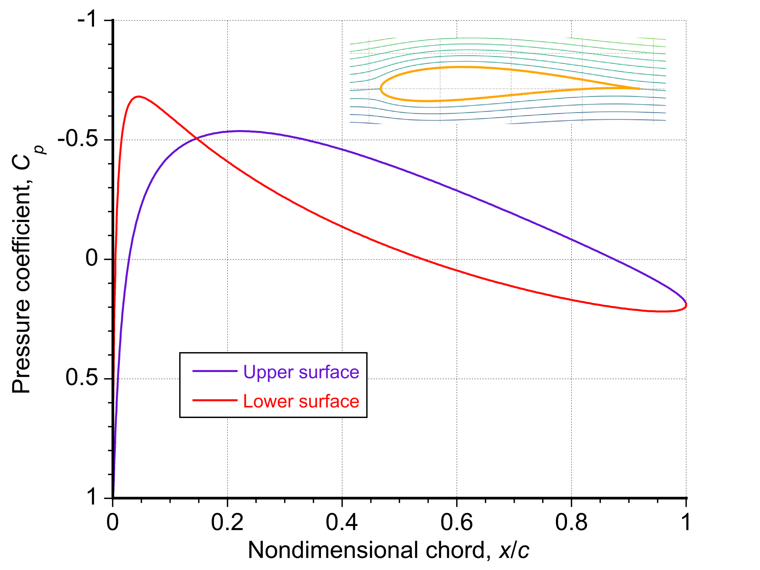 versus chordwise position for a Joukowsky airfoil with offsets
  and
and  .
.Forces and Moments from Complex Potential Theory
Now consider the lifting cases, which require the consideration of circulation. In two-dimensional potential flow, the velocity field around a body can be expressed using a complex potential  , where is the velocity potential and is the stream function. The complex conjugate velocity is given by
(183) 
This formulation allows the total force on a closed contour enclosing the body to be evaluated using complex-variable methods. The two key results that are central to the process are Blasius’ theorem, which gives the force and moment directly in terms of the complex velocity, and Cauchy’s integral theorem, which supports the derivation and application.
Blasius Theorem
Let be a positively oriented (counterclockwise) contour around a closed body in two-dimensional incompressible, irrotational, inviscid flow. The resultant force  (drag plus
  lift) exerted by the fluid on the body is given by
(184) 
Here, is the complex velocity, and  is the differential along the contour in the complex plane. This elegant result avoids direct pressure integration and is valid for any analytic potential flow field.
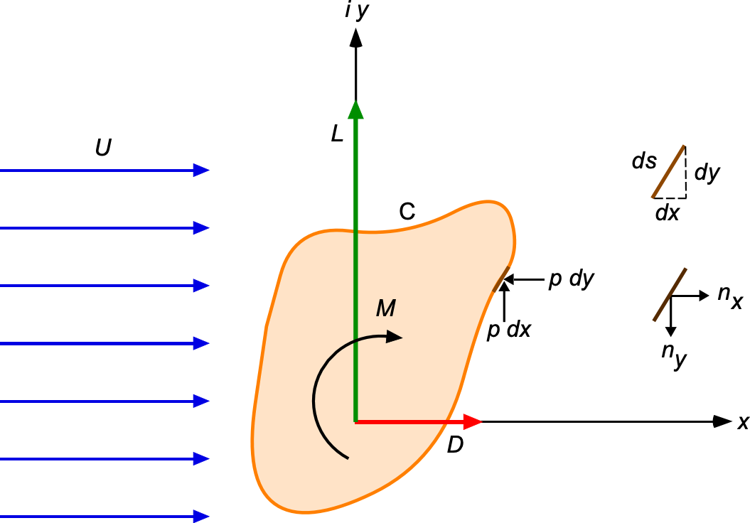
To understand its origin, recall that the force on the body arises solely from the pressure acting normally to the surface. For a smooth surface in two dimensions, the differential force element is
(185) 
where  is the pressure,
  is the outward-pointing unit normal vector, and
  is the arc length element along the contour C. The total force components are then
(186) 
Using the geometric relationships for the outward normal, i.e.,
(187) 
this becomes
(188) 
The complex force is therefore
(189) 
Noting that  , where
  , the force becomes
(190) 
The Bernoulli’s equation for steady, incompressible, irrotational, inviscid flow is
(191) 
where  is the ambitent static pressure and
  is the total pressure. Therefore,
(192) 
Introducing the complex velocity given by  gives
gives
(193) 
and so
(194) 
Substituting into the expression for  gives
gives
(195) 
The integral of the constant term vanishes around the closed contour, i.e.,
(196) 
so the result simplifies to
(197) 
Under the assumption that is analytic around the contour C, then
(198) 
The corresponding moment about the origin (positive clockwise) is similarly given by
(199) 
These expressions apply to flows composed of elementary singularities, such as sources, vortices, and doublets, to be superimposed analytically.
Cauchy’s Integral Theorem
If  is analytic inside and on a simple closed contour C, then by Cauchy’s theorem,
(200) 
Consider the integrand  and let the contour C represent the boundary of a body in the complex plane. This curve C can now be enclosed by a larger, positively oriented circle of radius centered at the origin, as shown in the figure below.
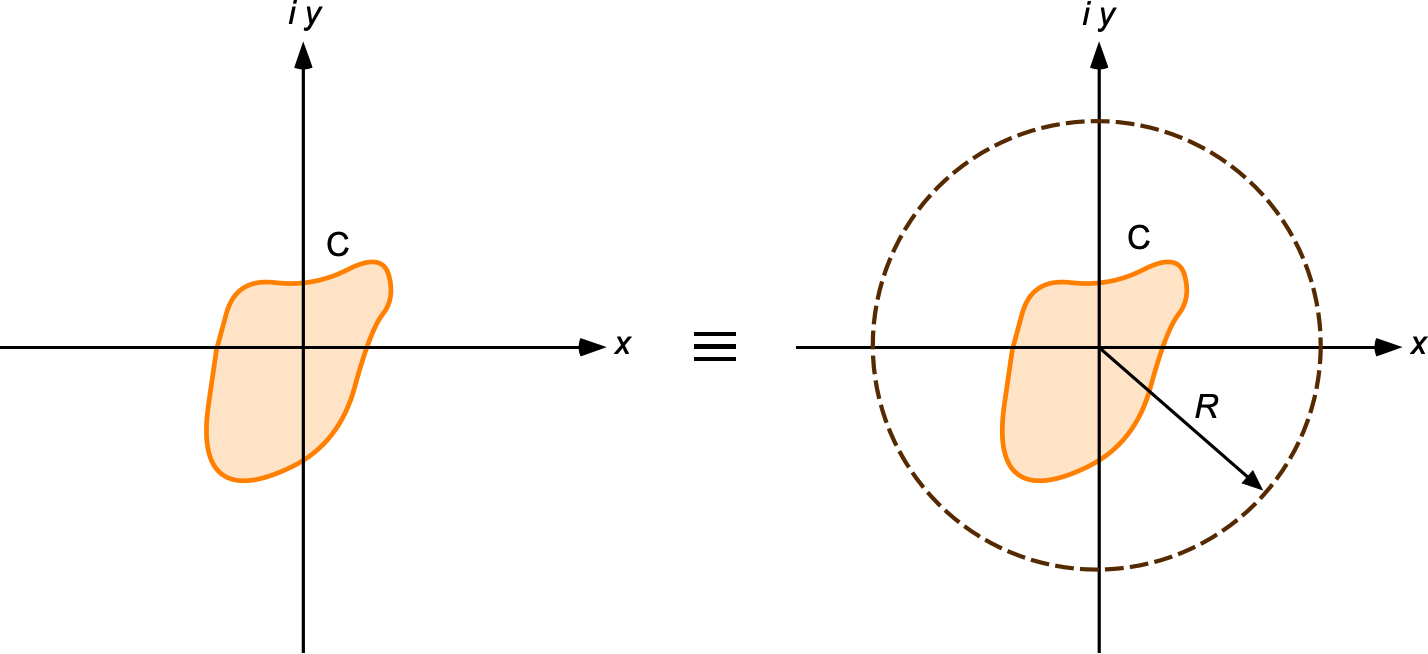
If  , then the integral over any contour enclosing the origin evaluates to
(201) 
because  is a simple pole enclosed by the contour. This reflects the residue of the singularity at the origin. For all other integer values
  , the function
  is analytic at , and so
(202) 
This example illustrates how the nonzero value of the integral arises exclusively from the singularity structure of the integrand within the contour. In aerodynamic applications, such singularities correspond physically to elements like point vortices or sources within the flow domain. The enclosing circular contour of radius provides a convenient analytic boundary for invoking Cauchy’s theorem or evaluating residues, while the body contour C may lie anywhere inside this outer domain.
These results are beneficial when combined with conformal mapping techniques. By constructing the potential flow in a simpler geometry and mapping it to a physical airfoil shape, the Blasius and Cauchy theorems enable direct calculation of aerodynamic forces from the transformed velocity field, without requiring pressure integration over the physical surface. This framework underpins classic airfoil theory, including the conformal transformation method and thin airfoil theory, which are considered in the next chapter.
Lift on Joukowsky Airfoils using Blasius’ Theorem
Consider again a Joukowsky airfoil generated by the mapping of a circular cylinder (or circle) in the -plane to the -plane using the transformation
(203) 
The circle has radius , and its center is offset slightly from the origin to introduce camber. The flow in the -plane consists of a uniform freestream , inclined at angle , and a vortex of circulation . The complex potential in the -plane is
(204) 
The complex velocity is
(205) 
To compute the lift, apply the Blasius theorem in the mapped -plane, i.e.,
(206) 
However, because , and , the chain rule is used to get
(207) 
Therefore,
(208) 
because  . Therefore, the Blasius integral becomes
(209) 
Notice that the only singularity of  inside the contour is the vortex.
The residue theorem is then used to give
(210) ![\begin{equation*} F = \pi \, i \varrho \, \text{Res}_{\zeta = 0} \left[ \left( \frac{d\widetilde{w}}{d\zeta} \right)^2 \right] \end{equation*}](https://eaglepubs.erau.edu/app/uploads/quicklatex/quicklatex.com-7eced1c69a431d64a511151e986d32ec_l3.svg "Rendered by QuickLaTeX.com")
Near , the dominant term in is  giving
(211) 
However, the full residue must be obtained, including cross terms, so that
(212) 
The only term with a simple pole at is the cross term, i.e.,  , so that
(213) 
Therefore, the total force is
(214) 
Separating into components, recall  , so that
(215) 
(216) 
If is small (as is typically assumed in airfoil theory), the drag is negligible, and the lift is
(217) 
This equation will be recognized as the well-known Kutta-Joukowsky theorem for lift, derived cleanly from a conformal mapping and the use of Blasius’ integral theorem.
General Method of Singularities
Consider now a general method of singularities for modeling two-dimensional potential flows. An understanding of this method is important because it provides a foundation for more advanced numerical techniques for flow analyses, particularly panel methods, which are considered in a later chapter of this eBook.
In the method of singularities, the flow is modeled as a superposition of idealized point singularities such as sources, sinks, vortices, and doublets, each with known analytical potential and velocity fields. Hence, panel methods may be viewed as a numerical implementation of the method of singularities whe it is applied to arbitrary body shapes with specificed boundary conditions. Panel methods retain the advantages of potential flow theory while enabling the accurate modeling of the flow about realistic aircraft geometries.
Let the flow be composed of a uniform freestream at an angle of attack to the body axis, with an arbitrary number of singularities, including sources, sinks, vortices, and doublets enclosed within a closed boundary, as shown in the figure below. The total complex potential at a point  can be written as
(218) 
where  is the strength of the
  -th source or sink (positive for source),
  is the strength of the -th vortex (positive counterclockwise),
  is the strength of the -th doublet,
  is its orientation angle, and
  is the location of the -th singularity in the complex plane. Notice that a physical flow constraint for a closed body is
(219) 
which ensures mass conservation.

Differentiating the complex potential for this flow gives the complex velocity, i.e.,
(220) 
At large distances where  , each term can be expanded in powers of
  , i.e.,
(221) 
Substituting these into , the expansion becomes
(222) 
with
(223) 
which represents the effects from the sources and vortices. The next coefficient is
(224) 
which includes the effects of the doublets.
Aerodynamic Force
The net complex force per unit span can be obtained using the Blasius theorem, i.e.,
(225) 
where is a closed contour enclosing all singularities. Using the previous expansion with some algebra, then
(226) 
where  represents the first-order contribution from sources and vortices, and
  represents higher-order terms that come from the interaction of sources, vortices, and doublets. The Cauchy residue of this function at
  is
is
(227) 
so the force becomes
(228) 
noting that only the sources and vortices contribute to the net force. Therefore, the force components are
(229) ![\begin{align*} X &= 2\varrho \, U \, \Re \left\{ A_1 e^{-i\alpha} \right\} = 2\varrho \, U \left( \sum_{k=1}^{N_s} \frac{Q_k}{2\pi} \cos\alpha + \sum_{k=1}^{N_v} \frac{\Gamma_k}{2\pi} \sin\alpha \right) \\[8pt] Y &= -2\varrho \, U \, \Im \left\{ A_1 e^{-i\alpha} \right\} = 2\varrho \, U \left( \sum_{k=1}^{N_s} \frac{Q_k}{2\pi} \sin\alpha - \sum_{k=1}^{N_v} \frac{\Gamma_k}{2\pi} \cos\alpha \right) \end{align*}](https://eaglepubs.erau.edu/app/uploads/quicklatex/quicklatex.com-e6d5726319c4645714add6c667342ed7_l3.svg "Rendered by QuickLaTeX.com")
where
(230) ![\begin{align*} \Re\left\{ \frac{Q_k}{2\pi} e^{-i\alpha} \right\} &= \frac{Q_k}{2\pi} \cos\alpha & \Re\left\{ \frac{-i \Gamma_k}{2\pi} e^{-i\alpha} \right\} &= \frac{\Gamma_k}{2\pi} \sin\alpha \\[6pt] \Im\left\{ \frac{Q_k}{2\pi} e^{-i\alpha} \right\} &= \frac{Q_k}{2\pi} \sin\alpha & \Im\left\{ \frac{-i \Gamma_k}{2\pi} e^{-i\alpha} \right\} &= -\frac{\Gamma_k}{2\pi} \cos\alpha \end{align*}](https://eaglepubs.erau.edu/app/uploads/quicklatex/quicklatex.com-f2c7b01502fa8cb02d66ac3808abb080_l3.svg "Rendered by QuickLaTeX.com")
For a closed body  to satisfy continuity, so the contributions from the sources are eliminated, i.e.,
(231) 
Lift
The lift per unit span is the component of the total aerodynamic force perpendicular to the freestream direction. If the freestream velocity makes an angle with the -axis, then
(232) 
Substituting the expressions for  and
and  for a closed body, i.e., with , gives
(233) ![\begin{align*} L' &= -\left( 2\varrho \, U \sum_{k=1}^{N_v} \frac{\Gamma_k}{2\pi} \sin\alpha \right) \sin\alpha + \left( 2\varrho \, U \sum_{k=1}^{N_v} \frac{\Gamma_k}{2\pi} \cos\alpha \right) \cos\alpha \\[8pt] &= 2\varrho \, U \sum_{k=1}^{N_v} \frac{\Gamma_k}{2\pi} \left( \cos^2\alpha + \sin^2\alpha \right) \end{align*}](https://eaglepubs.erau.edu/app/uploads/quicklatex/quicklatex.com-eb42f98e40f5feb8fad23cc81b25362f_l3.svg "Rendered by QuickLaTeX.com")
which simplifies to
(234) 
where  is the total circulation, defined as
(235) 
This is the classical Kutta-Joukowsky result where the lift per unit span is directly proportional to the total circulation induced by all of the vortices in the system.
Drag
The drag per unit span is the component of the total aerodynamic force in the direction of the freestream velocity. If the freestream velocity makes an angle with the -axis, then
(236) 
Substituting the expressions for and for a closed body, i.e., , then
(237) ![\begin{align*} D' & = \left( 2\varrho \, U \sum_{k=1}^{N_v} \frac{\Gamma_k}{2\pi} \sin\alpha \right) \cos\alpha + \left( -2\varrho \, U \sum_{k=1}^{N_v} \frac{\Gamma_k}{2\pi} \cos\alpha \right) \sin\alpha \\[8pt] &= 2\varrho \, U \sum_{k=1}^{N_v} \frac{\Gamma_k}{2\pi} \left( \sin\alpha \cos\alpha - \sin\alpha \cos\alpha \right) = 0 \end{align*}](https://eaglepubs.erau.edu/app/uploads/quicklatex/quicklatex.com-33bb57e6135907ea0069f59b5bcd0655_l3.svg "Rendered by QuickLaTeX.com")
Therefore, the drag force is identically zero in potential flow, i.e.,
(238) 
This result is consistent with all potential flows, i.e., the drag on a closed body is zero even though lift may be nonzero.
Prandtl-Glauert Compressibility Rule
At the beginning of the 20th century, advancements in analytical methods of aerodynamics and fluid mechanics assumed that the flow was incompressible. However, this assumption breaks down as the freestream Mach number exceeds about 0.3. During the 1920s, Ludwig Prandtl and Hermann Glauert independently discovered that, for subsonic flows around relatively thin airfoils with small perturbations, compressibility effects can be accounted for by a simple geometric mapping of the flow field.[7] The procedure, now known as the Prandtl-Glauert transformation, enables the use of an incompressible flow solution to predict the corresponding solution for a linearized, subsonic compressible flow.
For incompressible, irrotational flow, the velocity potential, denoted by  , satisfies Laplace’s equation, i.e.,
(239) 
Many classical solutions in aerodynamics, such as those for point sources, doublets, thin-airfoil theory, and lifting-line theory, are derived from this equation. It is therefore attractive to retain these incompressible solutions and apply a correction for compressibility effects, rather than rederive new solutions directly from the compressible form of the governing equations.
Consider steady, inviscid, subsonic flow with small perturbations about a uniform freestream of velocity and freestream Mach number  . Linearising the small-disturbance potential equation and imposing the irrotationality condition gives
(240) 
Notice that this equation would reduce to Laplace’s equation if the first term were not multiplied by the factor  .
.
Define the compressibility factor as  and introduce a coordinate transformation given by
(241) 
Using the chain rule, the derivatives transform as  and
and  and similarly for the component. Substituting into Eq. 240 gives
(242) 
so that
(243) 
which is Laplace’s equation expressed in the transformed or “stretched”  coordinates. Therefore, under the assumptions of linearised subsonic compressible flow, the compressible velocity potential can be obtained from a known incompressible solution solved in the domain using
(244) 
where  , i.e., there is no scaling in the chordwise dimension. This approach forms the basis of the Prandtl-Glauert transformation, as summarized in the figure below for a two-dimensional airfoil section.
For incompressible flow, the linearised Bernoulli equation, kept to second order in the perturbation velocities, is
(245) 
For small-disturbance compressible flows, the corresponding isentropic form is
(246) 
Using the Prandtl-Glauert mapping gives
(247) 
In terms of the velocity components, then
(248) 
The pressure coefficient becomes
(249) 
and so
(250) 
Therefore, it can be seen from Eq. 245 that
(251) 
It can also be seen from the figure above that because the airfoil geometry appears at a higher angle of attack in the transformed (compressible) coordinates, i.e.,  , then the pressure values in the compressible solution will be greater than for the corresponding incompressible flow solution. The assumption here is that the thickness and camber of the airfoil do not affect the pressure distribution, which is an issue considered next in the Göthert transformation.
Finally, integrating the pressure distribution over the surface leads directly to the commonly-used Prandtl-Glauert correction for the force and moment coefficients, i.e.,
(252) 
which means they all increase by the factor  . The correction, therefore, represents the additional lift (and moment) that arises on an airfoil or a wing because compressibility effectively amplifies the aerodynamic loading. For example, consider a thin symmetric airfoil that has an incompressible lift‑curve slope of
  (
( 6.28) per radian. According to the Prandtl-Glauert rule, the compressible value of the slope is
(253) 
If  , then
  and
and  , so about a 25% increase compared to the incompressible value.
Göthert Transformation
When an airfoil is not reasonably thin, its thickness and camber will alter its pressure field in a way that the simple Prandtl-Glauert rule cannot model. Göthert demonstrated that the problem can still be reduced to the incompressible Laplace equation if both the geometry and the coordinates are scaled.[8] After applying the linear coordinate transformation
(254) 
the airfoil thickness distribution  and camber line
  also become distorted under the coordinate transformation. For example, the thickness distribution becomes
(255) 
so the airfoil appears physically too thick in the transformed, compressible flow domain, as shown in the previous figure. To restore geometric similarity, Göthert scaled the airfoil geometry as well, using
(256) 
so that in the transformed domain, the airfoil’s geometry remains consistent within the framework of the linearized flow assumptions. The result is that incompressible potential flow methods can still be used, even for airfoils with moderate thickness and camber.
In the Göthert transformation, the pressure coefficient still scales using the Prandtl-Glauert transformation as
(257)
However, the lift coefficient, which is a normalized integral of the pressure difference over the airfoil chord, is affected by the thickness and camber. The pressure difference from angle of attack itself scales with  , while the thickness and camber scale with
  . These effects combine, so the result is scaling laws of the form
(258) 
Notice that the pitching moment coefficient involves an additional factor of , which is from the transformation of the moment arm. These expressions in Eq. 258 tend to be more accurate than the simple Prandtl-Glauert correction when applied to airfoils with moderate thickness and camber. Yet, they still fall within the scope of the linearized theory.
Summary & Closure
Potential flow theory, which is rooted in the Laplace equation, provides a foundational framework for understanding and analyzing many aerodynamic flows under the idealized assumptions of inviscid, incompressible, and irrotational conditions. By utilizing the velocity potential and stream function, potential theory enables a mathematical representation of flow fields, offering a simplified yet powerful model for predicting aerodynamic behavior. The ability to superimpose elementary flows, such as uniform flow, sources, sinks, and vortices, makes potential flow theory a versatile tool for analyzing composite flow patterns and understanding the fundamental mechanisms of fluid dynamics.
Despite its advantages, the potential flow theory has significant limitations that limit its applicability to practical problems. However, potential flow theory remains an invaluable baseline model, and today, it can often be integrated with other methods that account for viscous and turbulent effects using various forms of viscous-inviscid coupling methods. These hybrid approaches can be compelling for analyzing and predicting flow behavior, bridging the gap between theoretical insights and practical engineering solutions. The Prandtl-Glauert transformation also provides a link between incompressible flow theory and subsonic compressible potential flow using a simple geometric transformation. It provides a convenient Mach number correction for lift, moment, and pressure coefficients and is a valuable predictive approach, provided the flow stays below the critical Mach number and the geometric and kinematic assumptions are respected.
5-Question Self-Assessment Quickquiz
For Further Thought or Discussion
- What are stagnation points, and why are they important?
- What are the key limitations of potential flow theory in capturing aerodynamic phenomena?
- How has potential flow theory evolved historically within the field of aerodynamics?
- How do predictions from potential flow theory compare with experimental aerodynamic results?
- How might potential flow theory be integrated with other models, such as a boundary layer, to improve predictions?
Other Useful Online Resources
To understand more about the aerodynamics of potential flows, explore some of these online resources:
- A good description of potential flow theory on Wikipedia.
- Potential flow theory as presented by MIT.
- Potential Flow: what it is and why it’s useful.
- Potential flow and Laplace’s equation – Engineering Mathematics at the University of Washington.
- Potential flow, stream functions, and examples – Engineering Mathematics at the University of Washington.
- This chapter is mainly taken from the author's fluid mechanics course notes as a student, the lectures being delivered by Professor Roderick Galbraith. Professor Galbraith is an Honorary Senior Research Fellow in the Division of Aerospace Sciences at the University of Glasgow, renowned for his work in low-speed unsteady aerodynamics. The former Shoda Professor of Aerospace Systems and a Fellow of the Royal Society of Edinburgh, Professor Galbraith has made significant contributions to the understanding of dynamic stall, rotorcraft aerodynamics, and wind turbine performance. He obtained his Ph.D. from the University of Cambridge under the advisement of Prof. M. R. Head. His career has focused on the physics of separated and reattaching flows, with applications in both aerospace and wind energy systems. ↵
- Stokes, G., “On the Steady Motion of an Incompressible Fluid,” Transactions of the Cambridge Philosophical Society, 1842. ↵
- Rankine, W. J. M., "On Plane Water-Lines in Two Dimensions, Philosophical Transactions of the Royal Society of London, Vol. 154, 1864, pp. 369–391. ↵
- Rankine, W. J. M., "Principles Relating to Stream Lines," The Engineer, October 16, 1868. ↵
- Conformality is a local property, which means that it applies to small, infinitesimally sized shapes. A conformal mapping might distort the overall shape of a larger area, but it will preserve the angles within that area. ↵
- Zhukovsky, N. E., "Über die Konturen der Tragflächen der Drachenflieger," Trudy TsAGI, 1906–1910 (various parts. ↵
- Prandtl, L., "General Considerations on the Flow of Compressible Fluids," NACA Technical Memorandum 805, 1936. English translation of: Prandtl, L. Allgemeine Überlegungen über die Strömung zusammendrückbarer Flüssigkeiten, Convegno di Scienze Fisiche, Matematiche e Naturali, Tema: Le Alte Velocità in Aviazione, Reale Accademia d’Italia, Fondazione Alessandro Volta, Rome, Italy, Sept. 30–Oct. 6, 1935. ↵
- Göthert, B. H., “Plane and Three-Dimensional Flow at High Speeds,” NACA Technical Memorandum 1105, 1946. English translation of: Göthert, B. H., Ebene und räumliche Strömung bei hohen Unterschallgeschwindigkeiten, Lilienthal-Gesellschaft für Luftfahrtforschung, Bericht 127, 1940. ↵
