64 Helicopters
Introduction[1]
Helicopters are a type of Vertical Take Off and Landing (VTOL) aircraft. They can take off and land from almost anywhere on the ground or at sea, hover motionless in the air, and then fly in any direction at the pilot’s whim. VTOL capability in an aircraft, also known as a runway-independent aircraft, is a tremendously valuable aviation asset. However, there is a significant price to pay for VTOL capability, including engineering complexity, limited flight range and endurance, and other compromised flight capabilities, as well as much higher acquisition and operational costs.
The development of the helicopter, a type of rotorcraft, lagged behind that of successful airplanes by almost 30 years. The success of helicopters can be attributed to the continued advancement of aeronautical technologies and scientific understanding. Over time, they have evolved into technologically advanced aircraft with many valuable capabilities that are crucial in multiple roles, including in civil and military service. The versatility and unique capabilities of helicopters have made them indispensable aircraft for rescue operations, medical evacuation, surveillance, policing, border patrol, and defense. Today, any military service would fail to function without access to the helicopter’s unique capabilities.

Modern helicopters utilize cutting-edge aerospace technologies to enhance performance, safety, and efficiency. Advances in aerodynamics have improved flight performance, while composite materials have reduced weight and enhanced structural durability. Fly-by-wire (FBW) flight control systems enable greater precision in hovering, station-keeping, and maneuvering flight, significantly improving operational capability. Health and usage monitoring systems (HUMS) also provide real-time tracking of a helicopter’s condition and performance, allowing for proactive maintenance strategies that extend service life and improve reliability. These innovations have solidified the helicopter’s role in aviation, ensuring continued advancements in rotorcraft technology.
Learning Objectives
- Know the history and challenges of developing a successful helicopter compared to an airplane.
- Better understand the factors that affect the hovering, climbing, and descending flight performance of helicopters and other rotating-wing aircraft.
- Understand the essential performance characteristics of a helicopter in forward flight and the factors that limit its capabilities.
- Appreciate how a helicopter is controlled during flight, including the use of blade hinges and cyclic blade pitch.
History
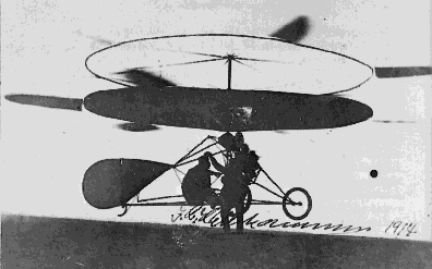
Jacob Ellehammer of Denmark was an aeronautical engineer and one of the pioneers of the helicopter; his coaxial-rotor machine was photographed in flight as early as 1913, as shown below. His machine made brief hops off the ground and short hovering flights, but could not fly forward or perform any useful tasks. In France, Paul Cornu and Louis Breguet also made notable attempts to build and fly helicopter concepts between 1906 and 1909, but these efforts were ultimately failures. The helicopter concepts built by Oehmichen, DeBothezat, and D’Ascanio during the 1920s were somewhat more successful, but their capabilities were marginal. Many other attempts were made to develop and fly helicopters over the following decade, but with only incremental success.
The first successful rotorcraft concept was not a helicopter, but a machine with an unpowered rotor called an autogiro, which would self-rotate or autorotate, creating lift as it flew forward, powered by a propeller. The name “autogiro” comes from the ancient Greek words αὐτός (auto) and γύρος (turning in a circle or forming a disk), essentially meaning a “self-turning” or “autorotating” rotor. “Autogiro” is a proprietary name coined by Cierva; however, all aircraft in this class are collectively known as “autogiros.” Today, the FAA refers to such aircraft as gyroplanes. Juan de la Cierva’s fourth attempt to build an autogiro resulted in the C-4, as shown in the photograph below, which first flew in 1923.
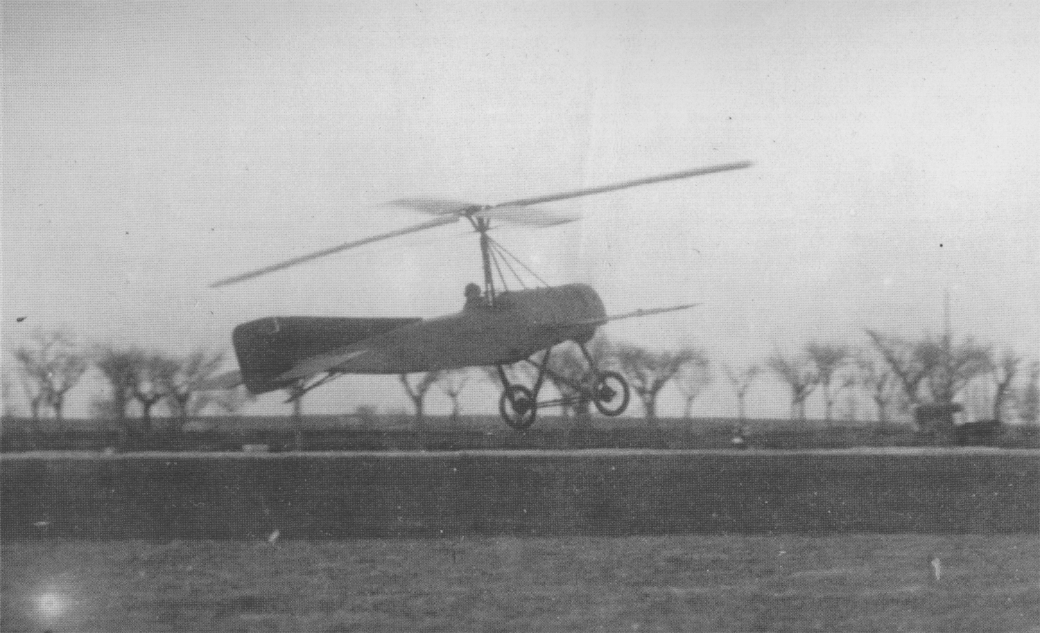
Besides discovering (or rediscovering) the principle of autorotation, Cierva’s primary innovation was the use of an independent flapping hinge that attached each blade to the rotating shaft, i.e., a pin joint. This design philosophy marked a fundamental departure from that used in propellers, where the blades are rigidly attached to the hub and cannot independently accommodate asymmetries in angle of attack or lift. The hinge allowed the blades to move freely up and down out of the plane of rotation (i.e., to flap) to help balance the asymmetric aerodynamic forces over the rotor disk during flight. While the autogiro could take off and land at very low airspeeds, essentially a stall-proof aircraft, it could not hover; the aircraft always required forward and/or downward motion through the air for the rotor to autorotate.
Through the mid-1930s, the autogiro demonstrated its usefulness in various military and civil missions, albeit with limited capabilities. Still, it was a helicopter with the ability to hover that was ultimately desired. Nevertheless, the autogiro proved an engineering platform for the helicopter’s future development. Of significance in the development of the autogiro was the development of not just flapping hinges, but also lead/lag hinges, which allowed in-plane movement of the rotor blades to alleviate Coriolis forces. Still, Cierva was not to take that critical step toward developing the helicopter.[2] To this end, notable engineering advancements were made by Raoul Hafner by finally integrating the successful elements of collective and cyclic blade pitch with flapping hinges on his AR-III gyroplane of 1935, developing what is known today as the fully articulated rotor system.
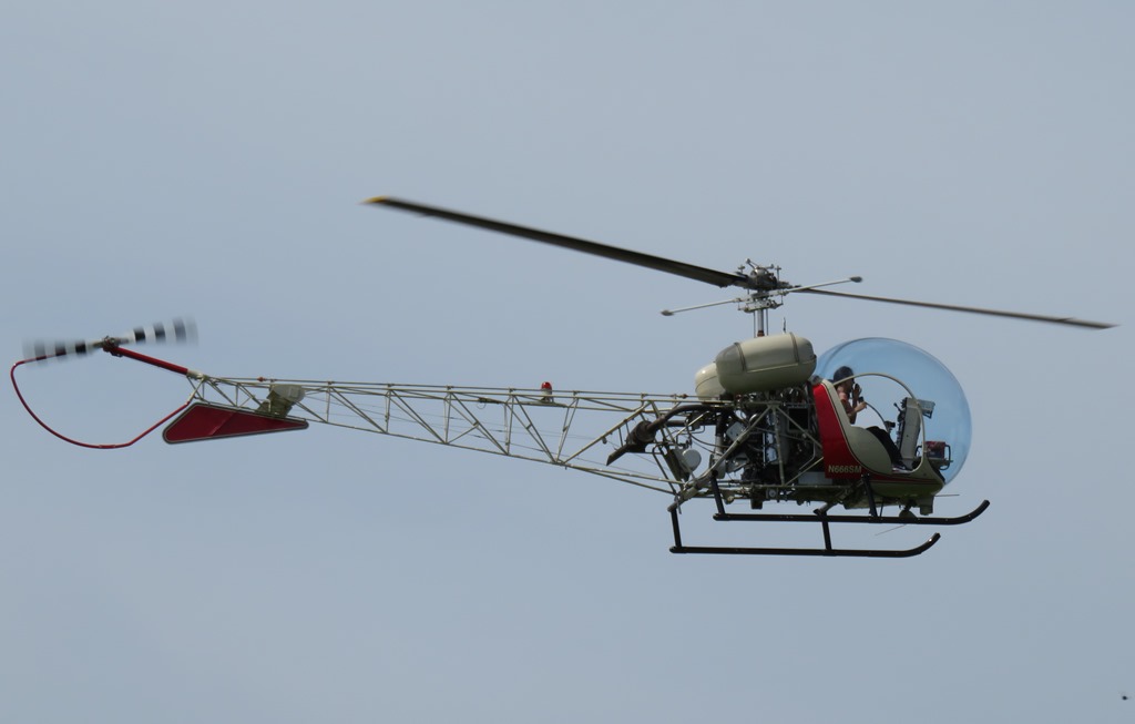
Before the outbreak of WWII, the first technically successful helicopters with fully articulated rotor systems had begun to appear, including the Gyroplane Laboratoire, the Focke-Wulf Fw 61, and the Sikorsky R-4. Germany utilized several types of helicopters during WWII, albeit in limited numbers. However, it was not until the late 1940s that helicopters became a significant part of the aviation spectrum for military and commercial use. To this end, numerous advancements in helicopter performance were made during the late 1940s and early 1950s. The first helicopters included the Bell-47, as shown in the photo below, the Bristol Sycamore, the Sikorsky S-55 and S-61, and the Vertol CH-46.
Sustained development in helicopter technology over the last half-century has led to numerous successful military and civil helicopter designs. During the 1970s and 1980s, many notable helicopters emerged. The Sikorsky UH-60 Black Hawk is an exemplary helicopter, having become one of the world’s most successful military helicopters and remaining in production to this day. The Boeing AH-64 Apache, first flown in 1975 and introduced in 1986, became the U.S. Army’s primary attack helicopter with its advanced avionics and Hellfire missiles. The Bell AH-1 Cobra and its upgraded Super Cobra variants continued to serve as effective attack helicopters, particularly with the U.S. Marine Corps.
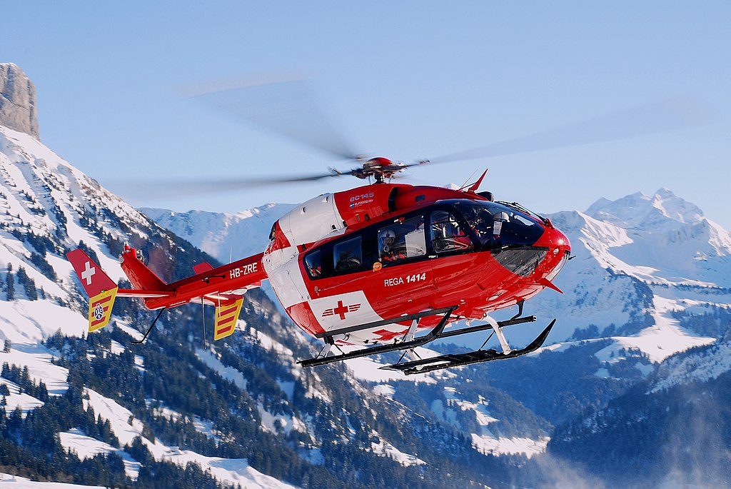
The British Westland Lynx, first flown in 1971, became a highly versatile helicopter used in both land and naval roles. Notably, it also set a world speed record for a helicopter in 1986, a record that remains unbroken to this day. The Eurocopter AS332 Super Puma, introduced in 1980, became a widely used transport helicopter for military and civilian operations. The Mil Mi-24 Hind, introduced by the Soviet Union in the 1970s, became a heavily armed and armored gunship capable of transporting troops and personnel. These helicopters played crucial roles in global military operations. Today, helicopters are increasingly constructed from advanced composite materials and incorporate numerous current aerospace technologies to enhance their performance, reliability, and safety. For example, the EC-145, as shown in the photograph below, is primarily built from composite materials, which provide the airframe with both strength and lightness. Indeed, modern helicopters have matured into sophisticated aircraft with extraordinary performance capabilities, and they play a unique role within the aviation spectrum that is unmatched by any other aircraft.
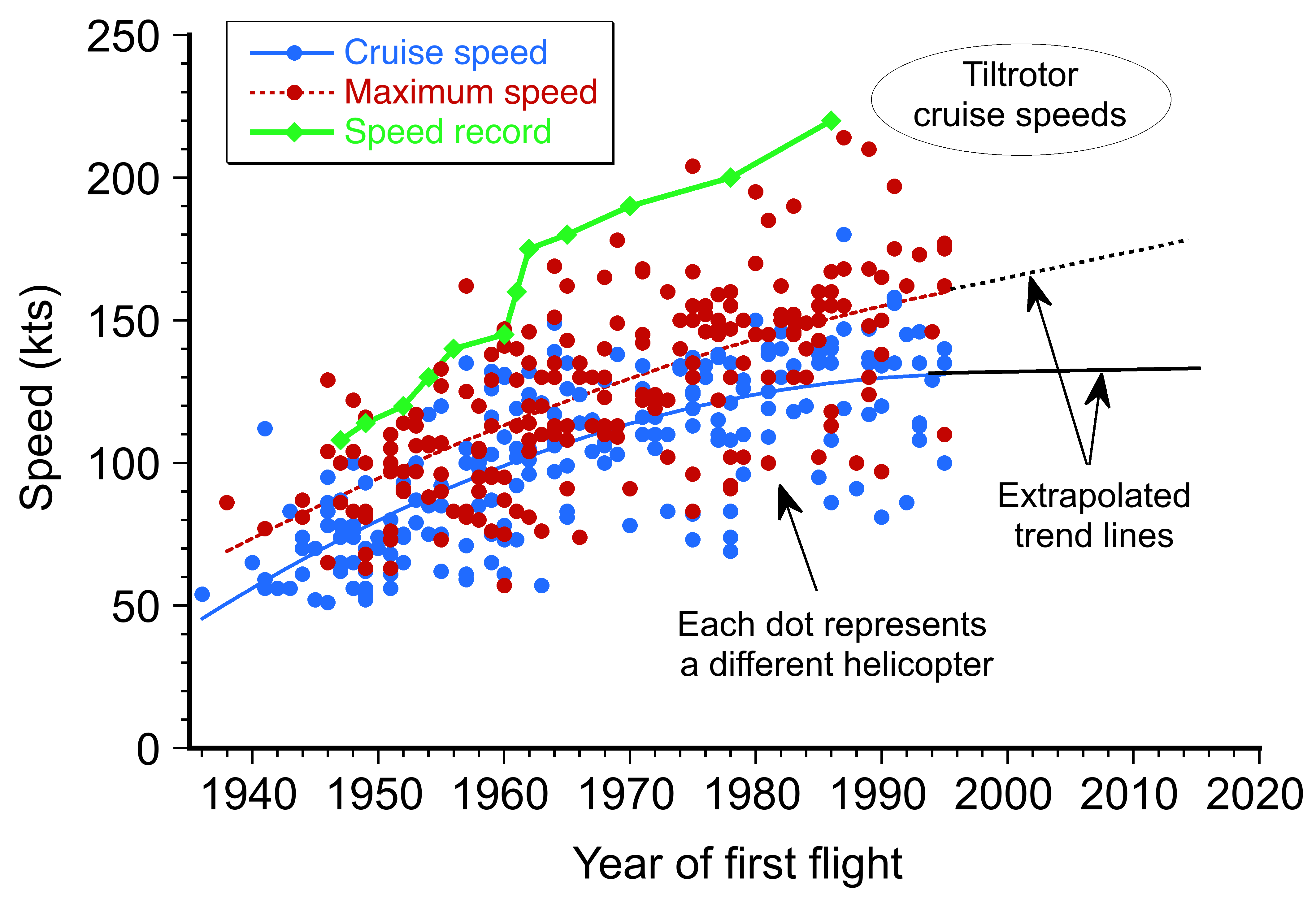
One issue with helicopters, however, is that they are inherently low-speed aircraft, with maximum airspeeds of only about 150 knots (173 mph, 278 kph), as shown in the figure below. This speed limitation is partly caused by the rotor system’s conflicting aerodynamic characteristics. Unlike an airplane, a helicopter’s rotor experiences both compressibility and stall effects simultaneously. Remember that an airplane typically experiences stall at low airspeeds and compressibility effects at high airspeeds; in this regard, the helicopter is unique.
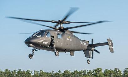
To overcome such inherent limitations, some helicopters have been equipped with auxiliary fixed wings or a separate propulsion system, known as compound helicopters. These systems can enable them to fly faster, but usually at the expense of increased power and fuel consumption, as well as a reduced payload. The Sikorsky S-97, as illustrated below, features variable-speed rigid coaxial main rotors and a variable-pitch pusher propeller, distinguishing it as a compound helicopter. The close spacing of the rotor hubs reduces drag in forward flight. The propeller relieves the rotor of propulsion demands, allowing the helicopter to achieve higher airspeeds.
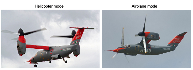
Hybrid rotorcraft such as the notorious Bell-Boeing V-22 Osprey and the long-awaited Leonardo/AgustaWestland AW609 (formerly the Bell/Agusta BA609) aim to combine the vertical takeoff and hover capabilities of helicopters with the increased speed and efficiency of airplanes. However, tiltrotors are not as effective as helicopters at performing tasks for which helicopters excel (e.g., hovering or operating at low airspeeds), and they also fall short of airplanes in certain areas (e.g., flying faster over longer distances while carrying a significant payload). Nevertheless, the V-22 Osprey tiltrotor has proven helpful for particular military missions. Whether the tiltrotor can succeed in the civil market remains to be seen, partly because its role is unclear, and, by any standard, it will have much higher acquisition and operational costs than an airplane or a helicopter.
Helicopter Configurations
Early helicopter concepts before 1930 featured the coaxial or side-by-side (lateral) rotor configuration; the various rotor configurations are illustrated in the figure below. The simplest idea of using a single main rotor with a smaller, sideward-thrusting tail rotor to compensate for torque reaction was not adopted until much later in the helicopter’s development. Nevertheless, the single main rotor/tail rotor configuration has since become the most common, comprising over 95% of all helicopters currently flying. The tandem rotor design is attractive for helicopters that require carrying a larger payload, as both rotors provide beneficial lift despite the greater mechanical complexity of gearing and controlling two rotors.
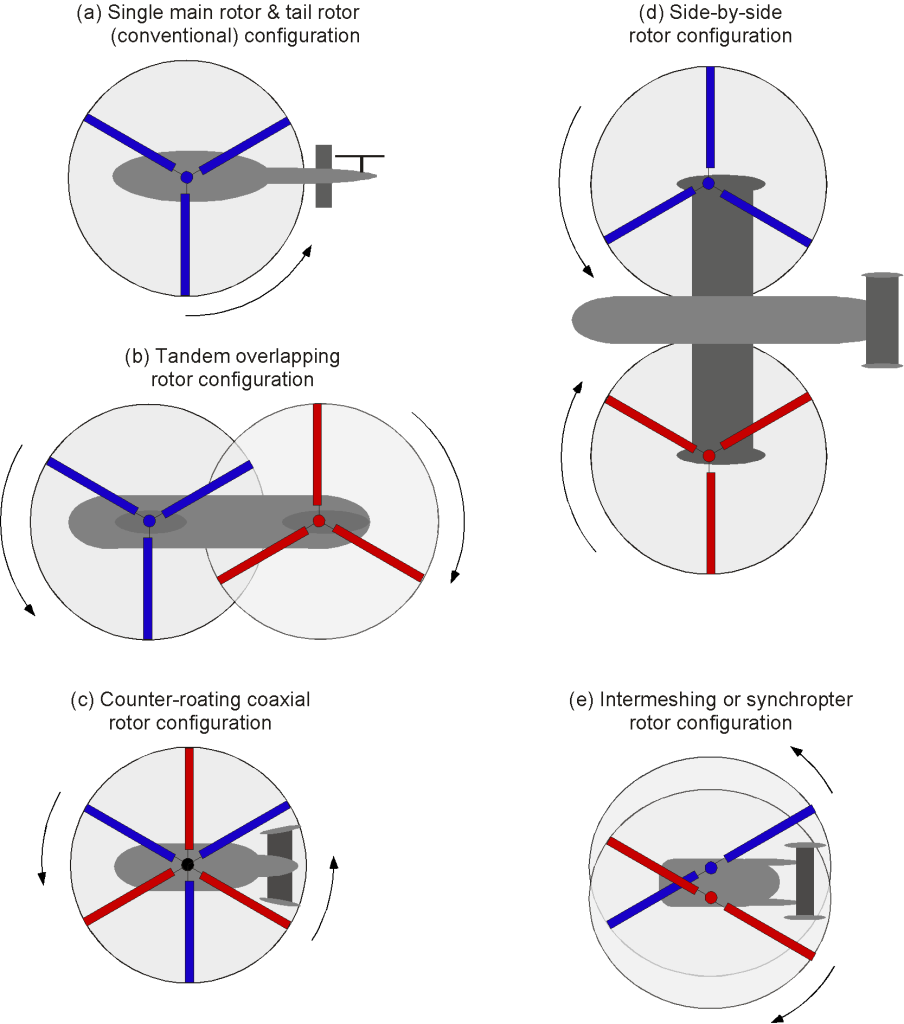
Contra-rotating “coaxial” rotors, with one rotor positioned above the other on a concentric shaft, automatically balance the torque reaction on the airframe, a helicopter configuration made famous laterally by the Kamov company. Another advantage is the compact footprint of the coaxial concept, despite its greater mechanical complexity. Side-by-side rotors, especially if the shafts were inclined inwards, gave the early machines somewhat better lateral stability, but the design is uncommon today. One notable example was the enormous Mil MV-12. Again, this type of design is more mechanically complex. The intermeshing design features outward-tilted, contra-rotating shafts with intersecting rotor disk planes, as seen on the Kaman K-Max. Like the coaxial, the intermeshing design offers a smaller overall footprint, which is beneficial for flight operations from confined locations.
Basis of Helicopter Flight
An airplane has separate lift, propulsion, and control systems, while a helicopter’s rotor system must perform all three functions. The rotor blades provide lift to overcome the helicopter’s weight, while the engine provides the power to spin the rotor and generate lift. The helicopter’s control surfaces, including the swashplate, pedals, and collective, enable control of its direction and altitude. This makes a helicopter’s design and operation more complex than an airplane’s, as the rotor system must perform multiple tasks simultaneously. Nevertheless, the helicopter’s unique ability to hover and fly vertically makes it ideal for many missions where a fixed-wing aircraft is impractical.
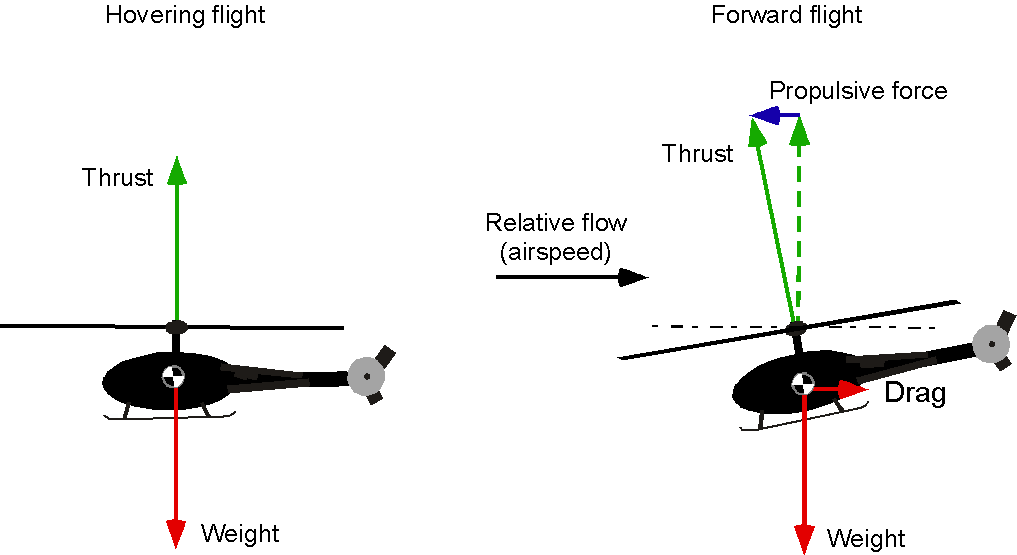
As shown in the figure below, the rotor generates a vertical lifting force (called thrust) that opposes the helicopter’s weight, produced by the collective lift of the spinning rotor blades. Generating a horizontal propulsive force for forward flight is achieved by tilting the rotor disk plane forward, providing a rotor thrust component to overcome the helicopter’s drag. This is accomplished by the pilot actuating the flight controls. The means of controlling a helicopter during its flight are discussed later.
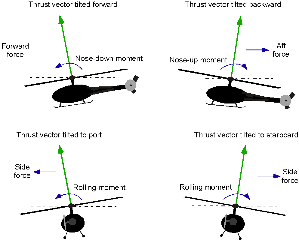
The rotor also generates forces and moments to help control the helicopter’s attitude and position in three-dimensional space. This behavior is obtained by tilting the orientation rotor disk left and right, as well as fore and aft, as shown in the figure below. Tilting the disk requires modulating the blade lift to cause flapping about the hinges, which results in a moment being applied through the hub and rotor shaft to the fuselage. So, the fuselage quickly aligns with the tilted rotor plane.
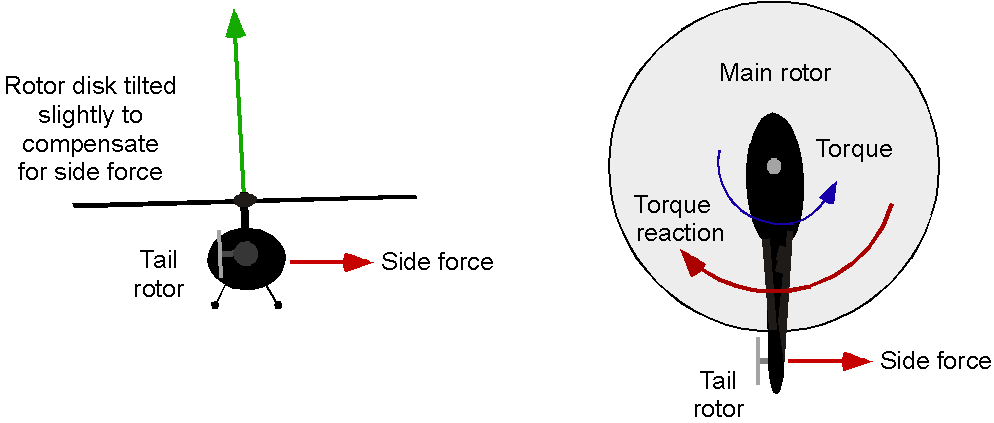
An anti-torque and yaw control system is necessary for a single-rotor helicopter, typically achieved through a tail rotor that generates sideward thrust. The pilot can modulate the tail rotor thrust for yaw control. In other rotor configurations, such as coaxial, tandem, and side-by-side, a tail rotor is unnecessary as the net torque reaction is already balanced. However, a slight residual torque reaction can be balanced by differential tilting of the two rotor disks, thereby creating a couple.
Rotor Flow Environment
The lifting capability of a lifting surface is related to its local angle of attack and flow velocity, specifically the dynamic pressure. In the case of a fixed (non-rotating) wing, the freestream velocity and the lift are relatively uniform along its span. However, in the case of a rotor, the flow velocity varies linearly along the span because of the rotation. The consequence is that the aerodynamic loads over the rotor disk are much more biased toward the blade tip, as shown in the figure below.
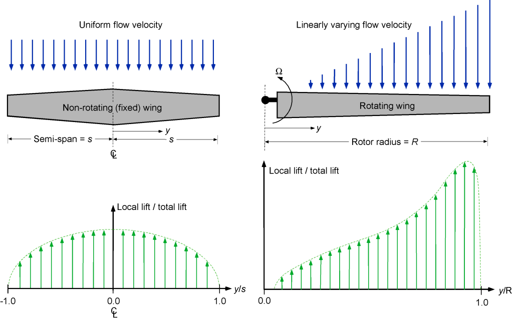
A fixed-wing aircraft must constantly move forward to generate lift. However, with a rotating wing or rotor blade, which can be assumed to be in hovering (non-translating forward) flight for now, lift can be generated without any “freestream” flow or forward motion. There will be no flow velocity at the rotational axis, but the flow velocity will increase linearly along the span of the blade. The velocity will reach a maximum at the blade tip,  , where
  is the rotor radius and
  is the rotor’s angular velocity. The consequence of the preceding is that a wing will have a reasonably uniform lift distribution, but a helicopter rotor will have a lift distribution that is much more biased toward the blade tips.
Asymmetry of Aerodynamics
When a rotor flies forward such that there is a component of a “freestream,” the flow over the rotor blades will no longer be axisymmetric about the center of the rotor, as shown in the schematic below. To explain the effects on the aerodynamics, the blade position can be defined in terms of an azimuth angle,  , which is defined as zero when the blade is pointing downstream, as shown in the figure below. Now, a component of the freestream,
  , adds to or subtracts from the rotational velocity at each part of the blade, i.e., for the tip section, then
(1) 
and at any radial position a distance  from the rotational axis, then
(2) 
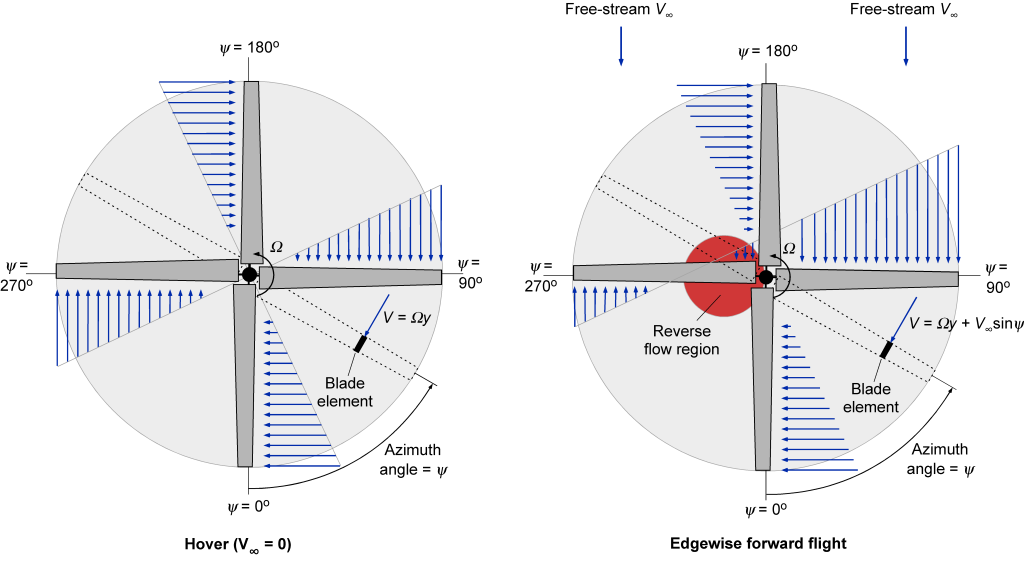
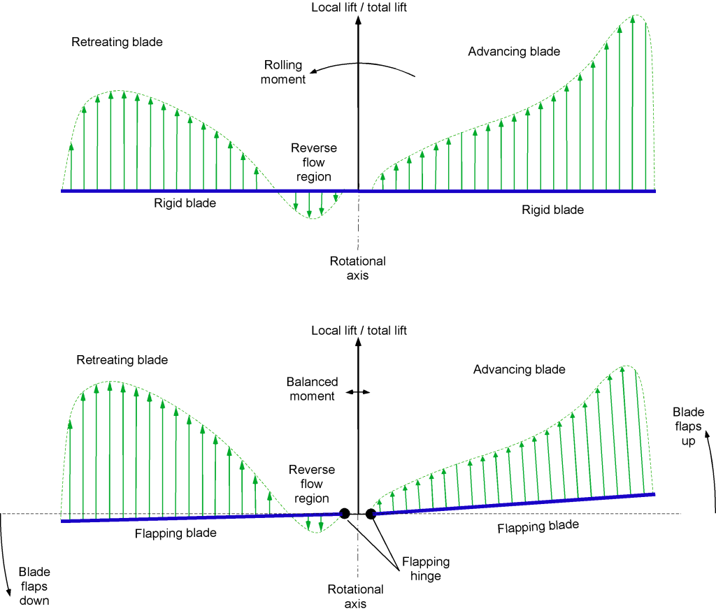
The consequence of this effect is that the rotor disk’s right side (the advancing side), where the blades advance into the freestream, will experience a higher overall flow velocity and dynamic pressure, resulting in increased lift. On the left (retreating) side of the rotor disk, where the blades move away from the freestream and dynamic pressure is lower, they will experience less lift. This problem, often referred to as the “dissymmetry in the lift,” was initially identified by Juan de la Cierva, as explained in the schematic below. Consequently, with blades that are rigidly attached to the rotor shaft, there will be substantial aerodynamic rolling moments on the rotor (turning the rotor toward its retreating side) that will make a rotorcraft of any kind impossible to fly. This problem was resolved by incorporating flapping hinges into the rotor system.
Blade Flapping
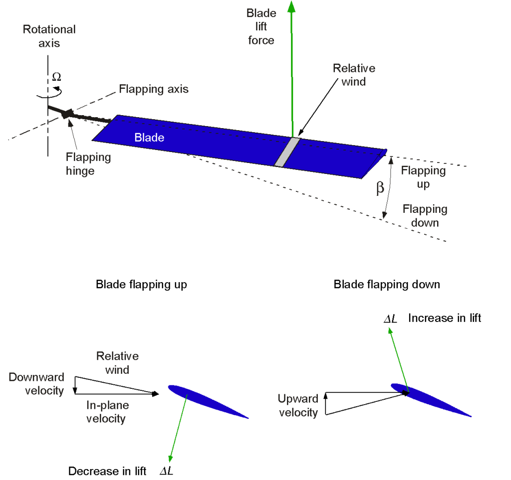
Cierva’s solution to this problem was to modulate the asymmetry in blade lift between the two sides of the rotor disk by using a pin-joint or “flap hinge” at the root of each blade, as shown in the figure above. This hinge allowed each blade to move up and down in response to the changing aerodynamic lift, as shown in the schematic below. The effects of blade flapping favorably alter the angles of attack, helping balance the distribution of aerodynamic loads across the rotor disk. On the advancing side of the rotor disk, where there is an excess of lift in response to the higher dynamic pressure, the blade flaps up about the hinge, decreasing the effective angle of attack and reducing lift, as shown in the schematic below. With a significantly lower dynamic pressure, the blade flaps down on the retreating side, thereby increasing lift on that side.
Therefore, a flapping hinge better balances the lift forces and moments generated on the advancing and retreating sides, resulting in a more uniform distribution over the entire rotor disk. Cierva referred to his invention of the flapping hinge as his “secret of success,” which allowed his C-4 autogiro to fly successfully in 1923.
Leading & Lagging
Cierva later introduced a “lead-lag” hinge to alleviate the in-plane inertia loads caused by Coriolis accelerations as the blade flaps up and down. This behavior occurs because, as the blade flaps up and down in the rotational plane, its center of gravity (or radius of gyration) shifts inward and outward relative to the rotational axis. Conservation of angular momentum results in Coriolis forces in the plane of rotation, which can induce significant structural stress on the rotor system. This fundamental behavior is illustrated in the figure below, which shows how a lead-lag motion is caused by blade flapping.
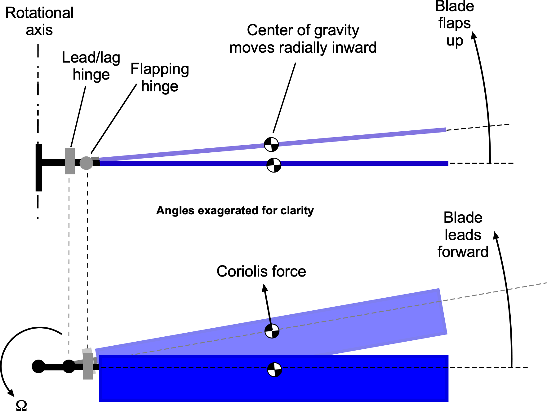
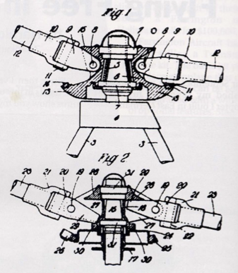
These issues came to a head with the Cierva model C.8, which suffered a catastrophic rotor failure during a test flight in 1927. One of its blades detached mid-flight because of excessive in-plane stresses acting on the rotor hub, a direct result of Coriolis-induced loads that were not fully understood at the time. To compensate for these forces, the lead-lag hinge allows the blade to move slightly forward and backward in the plane of rotation, dissipating the stresses that the hub structure would otherwise have to absorb. Without this hinge, excessive in-plane bending moments would be transferred to the rotor hub, potentially leading to high structural stresses that can cause fatigue and structural damage over time. Cierva patented the concept, as illustrated in the figure below, which proved to be a crucial step in the development of the fully articulated rotor system.
Blade Pitch
By further modulating the blade pitch angle or “feathering” angle, the lift on the blades can be adjusted so that the blades flap up or down at the appropriate location around the rotor azimuth, thereby causing the rotor disk plane as a whole to tilt left and right or fore and aft. Tilting the rotor disk gives a basis for controlling the orientation of the rotor thrust vector and the forces and moments acting on the helicopter as a whole. This is known as a fully articulated rotor system and proved crucial to the helicopter’s success as a viable form of aircraft.
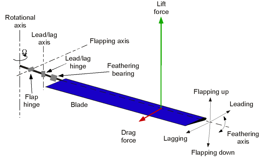
Depending on design requirements, the hinges and feathering bearings of a rotor system can be arranged in different sequences. A fully articulated rotor system typically includes:
- Flapping hinges – Allow blades to move up and down, compensating for the dissymmetry of lift.
- Lead-lag hinges – Enable in-plane motion to absorb Coriolis forces.
- Feathering bearings – Permit cyclic and collective pitch changes, which can be used to control the flapping of the rotor system.
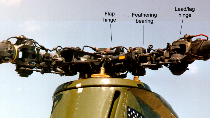
One example of a fully articulated rotor is shown in the photograph below, illustrating how these components are integrated into the rotor hub. In this particular arrangement, [describe notable features of the rotor in the image, e.g., the placement of lead-lag hinges, the orientation of feathering bearings, or any unique design aspects].
Rotor Wake & Blade Tip Vortices
One consequence of lift generation is that “tip vortices” form and trail from the tip of each rotating blade, just as they would trail from the tips of a wing. The figure below illustrates the physical nature of the vortical wake generated by a helicopter rotor in hovering flight, compared to that of an airplane. In each case, the tip vortices are rendered visible by the natural condensation of water vapor in the air, which leaves wispy white clouds in the flow behind the tips.
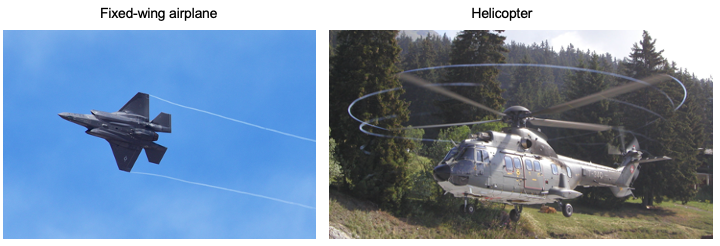
For an airplane, the vortices trail downstream and are left behind in the wake, never directly influencing the wing again. However, for a rotor, the vortices are convected downward below the rotor and form a series of interlocking, almost helical, trajectories. Therefore, the rotor blades can encounter their self-generated vortices as well as the vortices generated by other blades, which, overall, creates a much more complex flow environment at the rotor.
For this latter reason, predicting the strengths and locations of the tip vortices is essential for estimating blade airloads and rotor performance. The significant non-uniformity in the angles of attack experienced by the blade sections as they sweep around the rotor disk during edgewise forward motion is one complication with the helicopter rotor that makes its aerodynamic analysis difficult.
Hovering Flight Analysis
Unlike airplanes, helicopters can hover, a flight condition for which they are specifically designed to be operationally efficient. In hovering flight, the rotor’s primary purpose is to provide vertical lift to counter the helicopter’s weight. The thrust generation requires torque (and power) to be applied through the rotor shaft. In hover or axial flight, the flow is a nominally axisymmetric streamtube that passes through the rotor disk. This flow regime is the easiest to analyze initially, and, in principle, it should be the easiest to predict using mathematical models.
Although it is essential to remember that the actual physical flow through the rotor generates a complex vortical wake structure, as previously discussed, the rotor’s primary performance can be analyzed using a more straightforward approach known as momentum theory. This approach allows predictions of the relationships between rotor thrust and the power required to produce that thrust. Additionally, it reveals other parameters that can be used to assess rotor performance and efficiency, such as disk and blade loading.
Time-Averaged Flow Field
Hover is a unique flight condition where the rotor has zero forward (edgewise) speed and zero vertical speed (no climb or descent). A set of velocity measurements in a diametric plane near a hovering rotor and its wake is shown in the figure below. The flow velocity smoothly increases as it is entrained into and through the rotor disk plane. There is no jump in velocity across the rotor disk, although because a thrust is produced on the rotor, there must be a jump in time-averaged pressure over the disk.
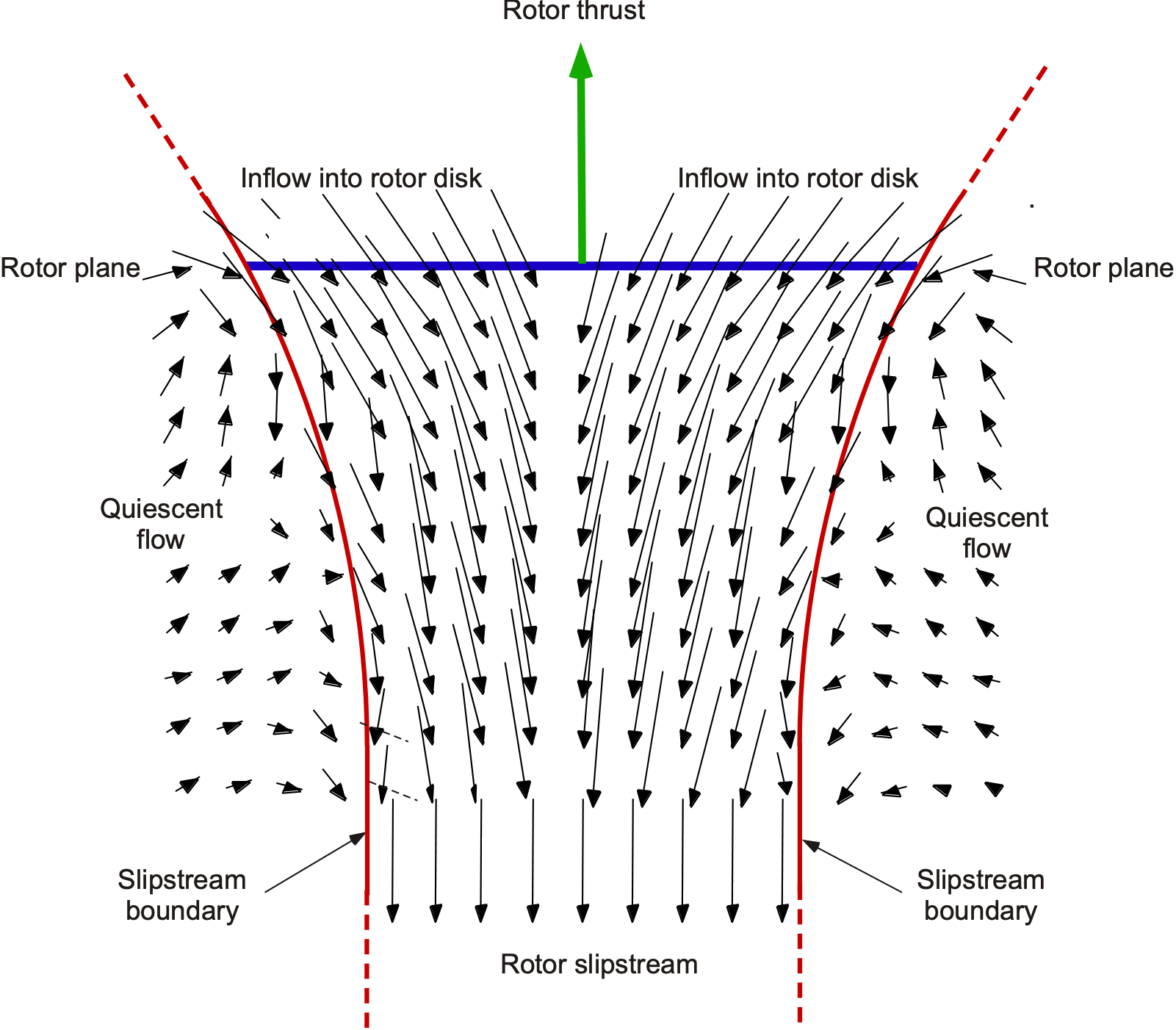
These measurements reveal a clear wake boundary, or slipstream, with the flow outside this boundary relatively calm or quiescent. Inside the wake boundary, the flow velocities are substantial and may be distributed non-uniformly across the streamtube and in the slipstream. Notice also the contraction in the diameter of the streamtube and wake boundary below the rotor, which corresponds to an increase in the slipstream velocity.
Flow Model
With the physical picture of the hovering rotor flow apparent, it is possible to develop a mathematical model. Consider the application of the three fundamental conservation laws (conservation of mass, momentum, and energy) to the rotor and its flow field. The conservation laws will be applied in a steady, incompressible, inviscid, axisymmetric, one-dimensional integral formulation to a control volume surrounding the rotor and its wake.
This simplified approach enables the most basic analysis of rotor performance (e.g., determining thrust produced and power required), but it does not account for the details of the flow environment or local conditions at each blade section. This approach, known as the momentum theory, was first developed by William Rankine in 1865 to analyze marine propellers and was formally generalized by Hermann Glauert in 1935 for application to helicopter rotors and autogiros. The assumptions are:
- One-dimensional, steady, incompressible, inviscid flow.
- The rotor is an infinitesimally thin disk that acts as a pressure discontinuity within the moving fluid.
- The disk offers no resistance to fluid passing through it.
- The pressure and velocity are uniform over the disk.
- The flow is at ambient static pressure far upstream and downstream of the rotor.
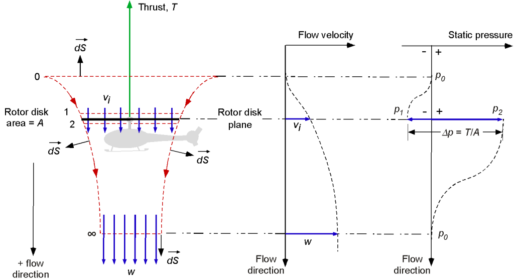
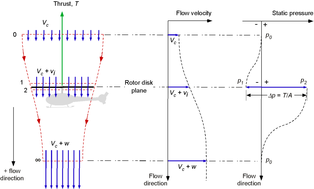
Consider the figure shown below. Let cross-section 0 denote the plane far upstream of the rotor, where the air is still or quiescent.  indicates the rotor disk area. Cross-sections 1 and 2 are the planes just above and below the rotor disk, respectively. The slipstream “far” wake is downstream of the rotor at
  . The flow through the rotor increases smoothly and continuously, although a jump in static pressure occurs over the disk, creating thrust.
A fundamental assumption in the momentum theory is that the rotor can be idealized as an infinitesimally thin actuator disk supporting a pressure difference; this concept is equivalent to an infinite number of thin, zero-thickness blades. This actuator disk supports the thrust generated by rotating blades about the shaft and their action on the air. The work done by the rotor on the air results in a gain in the flow’s kinetic energy in the rotor’s slipstream, an unavoidable energy loss, and a byproduct of thrust generation called induced power. According to Newton’s third law, the force exerted on the flow results in an equal and opposite force being produced on the rotor, i.e., the rotor thrust,  .
.
Application of the Conservation Principles
At the plane of the rotor, assume that the velocity there, which is called the induced velocity, is  . In the far slipstream, the velocity will be increased over that at the plane of the rotor, and this velocity is denoted by
  . The mass flow rate,
  , must be constant within the boundaries of the rotor wake, i.e., inside the control volume. The only cross-section of the wake boundary that is uniquely defined is at the rotor disk, so based on the assumed flow characteristics, then
(3) 
The principle of conservation of momentum relates the rotor thrust, , to the net time rate of change of the air’s momentum exiting the control volume (Newton’s second law). The rotor thrust is equal and opposite to the force on the air. For an unconstrained flow, the net pressure force on the air inside the control volume is zero, so the effects of external pressure can be neglected. Therefore, the rotor thrust can be written as
(4) 
From the principle of energy conservation, the work done on the rotor is equal to the gain in energy of the air per unit time. The work done per unit time, or the power consumed by the rotor, is  , so that
(5) 
From Eqs. 4 and 5 then it is apparent
(6) 
This latter result, therefore, gives a simple relationship between the induced velocity in the rotor plane, , and the velocity in the slipstream. Notice also that, based on ideal flow assumptions, the slipstream comprises an area that is precisely half of the rotor disk area.
The residual wake then expands gradually into the surrounding fluid, and the static pressure will approach the ambient pressure  even though the flow velocity remains finite. This behavior occurs because the flow carries residual momentum imparted by the rotor. So the velocity decays more slowly than the pressure recovers, which is required by the far-field boundary condition in most aerodynamic models.
Induced Velocity
The rotor thrust is related to the induced velocity at the rotor disk using
(7) 
Rearranging Eq. 7 to solve for the induced velocity gives
(8) 
Notice that  is used for the induced velocity in hover because it becomes a reference when the axial climb, descent, and forward flight conditions are considered. It is significant here that the ratio
  appears in Eq. 8, known as the disk loading, and it is a critical parameter in rotor analysis.
Power Required to Hover
The power required to hover, which is the time rate of work done by the rotor on the air, is given by
(9) 
This power value, called ideal power, is entirely induced in nature because the contribution of viscous effects has yet to be considered. In other words, this power value is the absolute lowest and, hence, the “ideal” amount required to generate a given rotor thrust.
Because  , it can also be written that
(10) 
This latter equation shows that the power required to hover will increase with the cube of the induced velocity  at the disk. Therefore, to make a rotor hover generating a given amount of thrust with the minimum power required, the induced velocity at the disk must be as low as possible. If is too low, then the rotor will generate no thrust because, for a given mass flow rate, then
(11) 
Therefore, to minimize the power required to produce thrust, the goal is that must be as low as possible, but the mass flow rate through the disk must be as large as possible. This goal consequently requires a large rotor disk area to entrain the required mass flow; large-diameter rotors are a fundamental design feature of all helicopters.
Pressure Variations
The pressure variation through the rotor flow field in the hover state can be determined by applying Bernoulli’s equation above and below the rotor disk. However, remember that there is a pressure jump across the disk because of the energy added by the rotor, so Bernoulli’s equation cannot be applied across the disk.
Referring to the previous figure, applying Bernoulli’s equation up to the rotor disk between stations 0 and 1 produces
(12) 
and below the disk, between stations 2 and , then
(13) 
Because the jump in pressure  is assumed to be uniform across the disk, this pressure jump must be equal to the disk loading, , that is
(14) 
Therefore, it can be written that
(15) 
From this, it can be seen that the rotor disk loading (i.e., the pressure) equals the dynamic pressure in the slipstream.
The pressure just above and below the disk can also be obtained in terms of disk loading. Just above the disk, the use of Bernoulli’s equation gives
(16) 
and just below the disk, then
(17) 
Therefore, the conclusion to be drawn is that the static pressure is reduced by  above the rotor disk and increased by
  below the disk, i.e., the net pressure jump is
  .
.
Check Your Understanding #1 – Distribution of thrust over the rotor disk
The simple momentum theory assumes that the pressure jump across the actuator disk of a hovering rotor is uniform and constant. By considering an elemental annulus of the rotor disk, prove that this result must be consistent with a distribution of lift (or thrust force grading) across the rotor disk that varies linearly from a value of zero at the center (rotational axis) of the rotor to a maximum value around the edges of the rotor disk.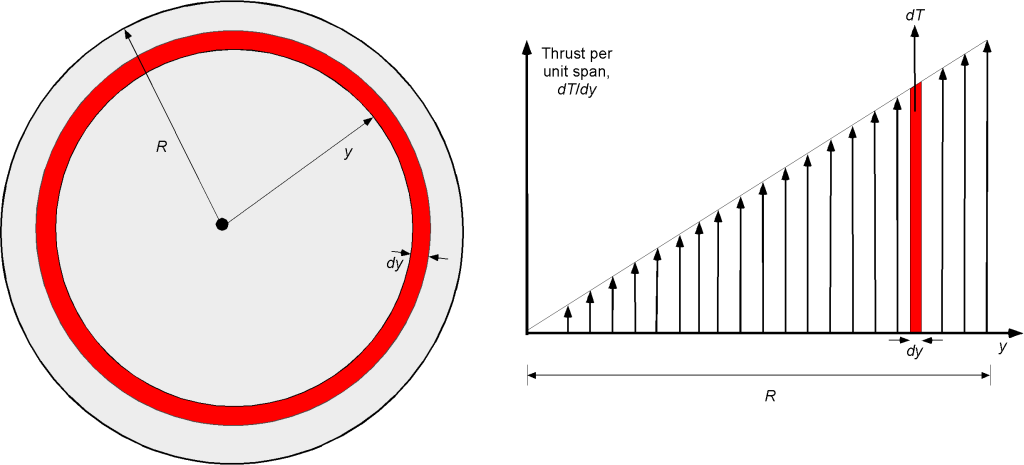
Show solution/hide solution.
The area of the elemental annulus is
![\[ dA = 2\pi y dy \]](https://eaglepubs.erau.edu/app/uploads/quicklatex/quicklatex.com-3d874cce113fa2df45328e1800a68863_l3.svg "Rendered by QuickLaTeX.com")
The rotor disk loading (a pressure) is
![\[ \frac{T}{A} = \Delta p = \mbox{constant} \]](https://eaglepubs.erau.edu/app/uploads/quicklatex/quicklatex.com-93160a93bc20e812acdc2e09f7dacf29_l3.svg "Rendered by QuickLaTeX.com")
where is the pressure jump over the disk. Therefore, the thrust  on the elemental annulus is
![\[ dT = \left( \Delta p \right)\, dA = \left( \Delta p \right) 2\pi y dy = 2\pi (\Delta p) \, y dy \]](https://eaglepubs.erau.edu/app/uploads/quicklatex/quicklatex.com-05603b15e017040b8a78e5217ba21a12_l3.svg "Rendered by QuickLaTeX.com")
Finally, the thrust per unit span or thrust distribution is
![\[ \frac{dT}{dy} = 2\pi (\Delta p) \, y \]](https://eaglepubs.erau.edu/app/uploads/quicklatex/quicklatex.com-862b53e7842f7dad2c0e36a05f15f9b5_l3.svg "Rendered by QuickLaTeX.com")
which is a linear distribution along the radial dimension of the rotor disk, extending from the rotational axis to the edge of the disk.
Disk Loading & Power Loading
A parameter frequently used in helicopter analysis that appears in the preceding equations is the disk loading, , denoted by  . Because for a single-rotor helicopter in a hover, the rotor thrust, , is equal to the helicopter’s weight,
  , the disk loading is sometimes written as
  or
or  . To compute the disk loading for multi-rotor helicopters, such as tandems, coaxials, or tiltrotors, a first assumption is that each rotor carries an equal proportion of the vehicle’s weight.
Disk loading is measured in pounds per square foot (lb ft ) in USC or Newtons per square meter (N m) in SI. In the SI system, the disk loading may also be quoted in kilograms per square meter (kg m). However, be aware that the direct use of the kilogram (kg) as a surrogate for a unit of force is strictly incorrect.
The power loading is defined as  and denoted
  . Power loading is measured in pounds per horsepower (lb hp
 ) in the USC system or Newtons per kilowatt (N kW) or kilograms per kilowatt (kg kW) in the SI system. Remember that the induced (ideal) power required to hover is given by
  . The ideal power loading is inversely proportional to the induced velocity at the disk, i.e.,
(18) 
According to the results in the figure below, the power loading,  , decreases quickly with increasing disk loading,
  ; notice the logarithmic scales. Therefore, vertical-lift aircraft with low effective disk loading will have relatively low power requirements per unit of thrust, i.e., a high power loading. This outcome means they will tend to be more efficient, i.e., the rotor will require less power and consume less fuel to generate a given amount of thrust.
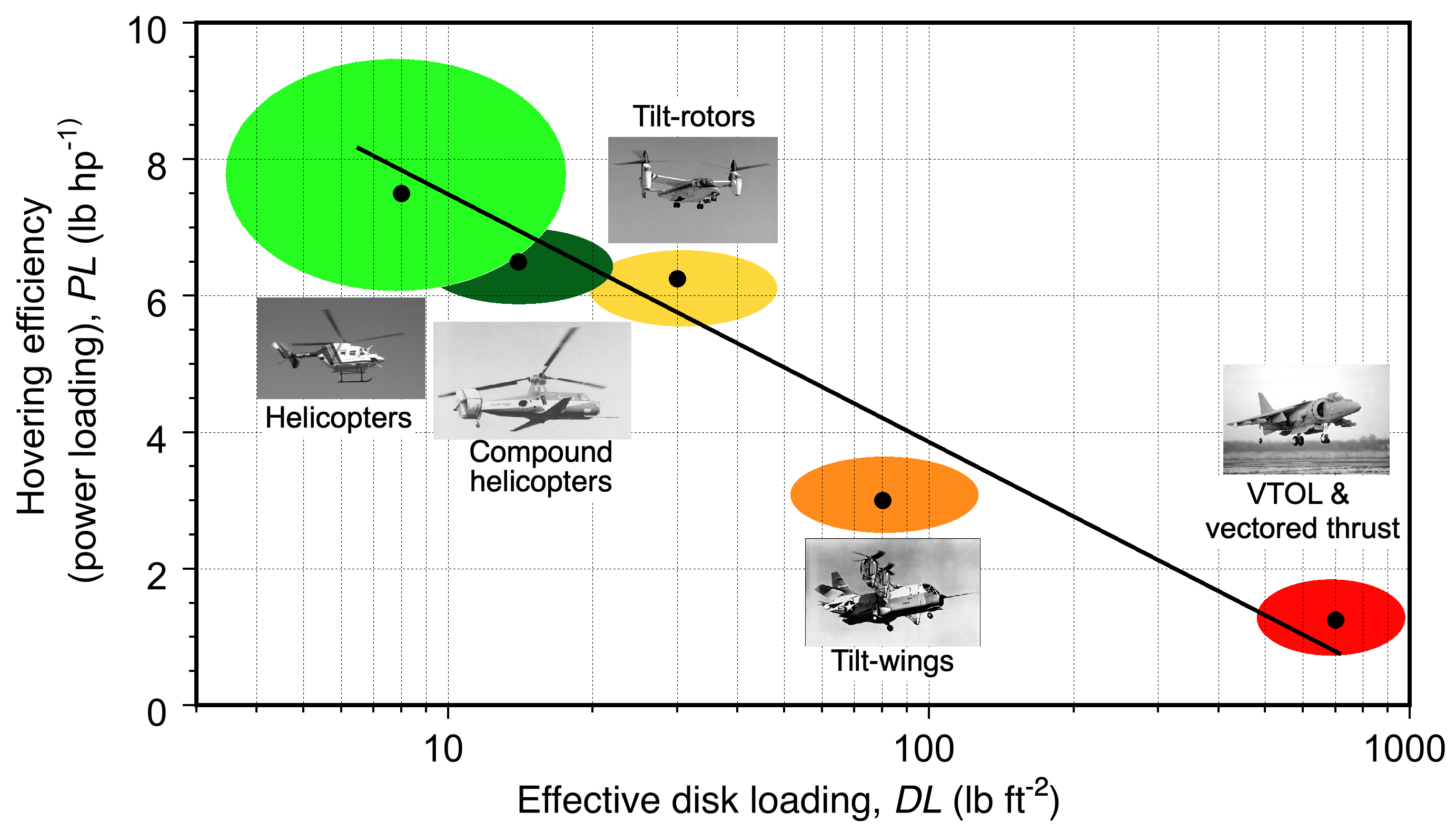
Helicopters operate with low disk loadings in the region of 5 to 10 lb ft or 24 to 48 kg m, so they can provide a large amount of lift for relatively low power with power loadings of up to about 5 kg kW (50 N kW or 10 lb hp). The above figure shows that the helicopter is a very efficient aircraft in hovering flight compared to other VTOL aircraft. Tiltrotors, because of their compromised design, have higher rotor disk loadings, making them less efficient than a helicopter of the same in-flight weight. Jet thrust concepts have very high effective disk loadings because of their high jet velocities and low exit areas.
Non-Dimensional Hovering Analysis
In rotor analysis, non-dimensional parameters are used to generalize aerodynamic performance for airfoils and wings. The non-dimensional value of the inflow,  , called the induced inflow ratio, is written as
(19) 
and in the hover case
(20) 
Recall that the angular or rotational speed of the rotor is denoted by , and is the rotor radius; the product is the tip speed, i.e.,  .
.
For helicopter rotors, it is the convention to non-dimensionalize all velocities by the blade tip speed in hovering flight  , and the reference area is the rotor disk area, . The rotor thrust coefficient is defined as
(21) 
Now it can be seen that the hover value of the inflow ratio,  , is related to the thrust coefficient by
(22) 
The corresponding rotor power coefficient is defined as
(23) 
Therefore, based on the momentum theory, the power coefficient for the hovering rotor becomes
(24) 
Again, this result is calculated based on a uniform inflow over the rotor disk and no viscous losses, which is referred to as the ideal power.
The corresponding rotor shaft torque coefficient is defined as
(25) 
Notice that because power  is related to torque
  by
by  , then numerically,
  has the same value as
  , although it would be incorrect to write that
  .
.
Measured Rotor Performance
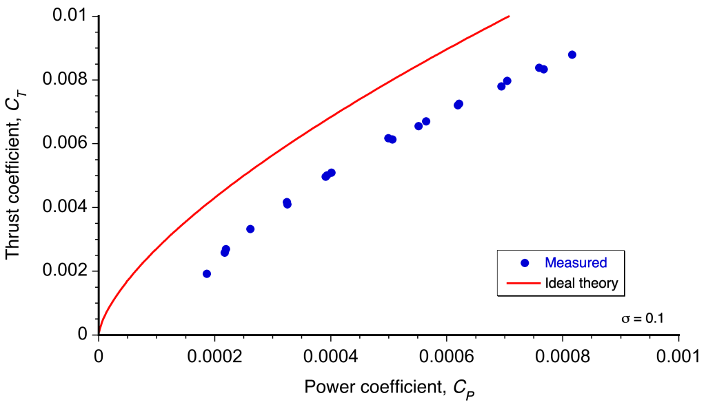
In terms of coefficients, the ideal power to hover according to the simple momentum theory can be written as
(26) 
The figure below compares Eq. 26 with thrust and power coefficient measurements made for a hovering rotor. The form of presentation is called a power polar and is analogous to the drag polar used for airplane wings. The momentum theory underpredicts the required power, but the predicted trend,  , is correct. These differences between the momentum theory and experiments occur because viscous effects (i.e., non-ideal effects) have not been included in the basic theory. However, this deficiency can be addressed by applying empirical corrections to the theory.
Non-Ideal Effects
Non-ideal but physical effects not included in the basic momentum theory include phenomena such as non-uniform inflow, tip losses, wake swirl, suboptimal wake contraction, and a finite number of blades, among others. One of the most significant contributors to non-ideal effects is “tip loss,” which reflects the fact that a lifting surface cannot create a finite lift at its tips; therefore, the lift on the blade decreases rapidly as the tip is approached. Generally, non-ideal effects can be split into lifting (induced) and non-lifting contributions.
Induced Effects
In the ideal rotor theory, then  . For an actual rotor,
  can be derived from rotor measurements or flight tests. For preliminary design, most helicopter manufacturers use their own measurements and experience to estimate values of . A typical average value is about 1.15. Values of can also be computed directly using more advanced blade element methods, where the effects of the actual flight condition can be more accurately represented. This issue is particularly significant in high-speed forward flight, where the increasing nonuniformity of the inflow from the reverse flow on the retreating blade must be accounted for.
Profile Drag Effects
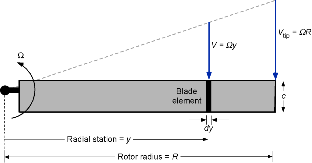
Estimates of the power profile consumed by a rotor require knowledge of the drag coefficients of the airfoils that comprise the rotor blades. Therefore, the drag coefficient will be a function of the Reynolds number and Mach number, varying along the span of the blade. However, a simple baseline result for the profile power can be obtained by summing the sectional drag forces element by element. i.e., the blade element method, as illustrated in the figure below.
The power required to spin the blade in the absence of thrust (i.e., the profile power,  ) can be obtained by radially integrating the sectional drag force along the length of the blade using
(27) 
where  is the number of blades, and
  is the drag force per unit span at a section on the blade at a distance from the rotational axis. The drag force on each blade element can be expressed conventionally as
(28) 
where  is the blade chord, which is assumed constant in this case, i.e., the blade has a rectangular planform.
If the section profile drag coefficient,  , is also assumed to be constant, i.e.,
  , then the profile power integrates to
(29) 
Converting this result to a power coefficient by dividing through by  gives
gives
(30) 
The grouping
(31) 
is known as the rotor solidity. Typical values of  for a helicopter rotor range between 0.05 and 0.12.
Modified Theory Versus Measurements
It is now possible to recalculate the rotor power requirements by using the modified momentum theory, such that
(32) 
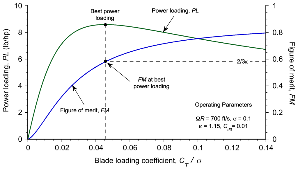
This result is illustrated in the figure below and calculated under the assumptions = 0.1, = 1.15, and  = 0.01.
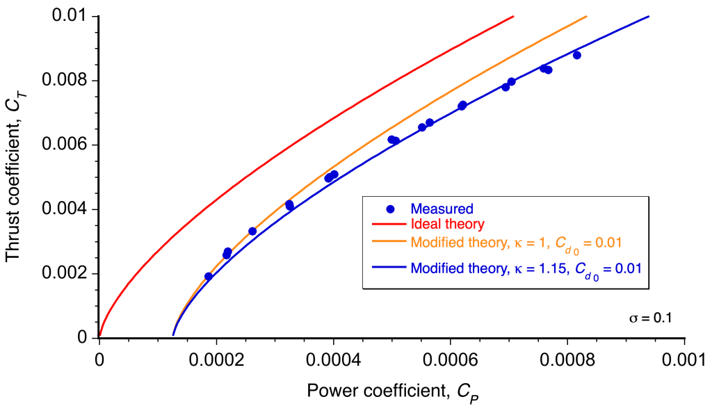
In the first case, to show the effect of adding profile power losses, it has been assumed that =1.0 (ideal induced losses), and in the second case, =1.15 (non-ideal losses). Notice the need to account for non-ideal induced losses and profile losses to give agreement with the measured data. The overall level of correlation thus obtained gives considerable confidence in the modified momentum theory approach for basic rotor performance studies, at least in hover.
Check Your Understanding #2 – Estimating power requirements for flight
In 1907, Paul Cornu built a primitive twin-rotor helicopter. Each rotor of his machine was approximately 19.7 ft in diameter. The machine had a net gross weight (with the pilot) of about 575 lb. Use momentum theory to verify the power requirements for flight, free of the ground and out of ground effect.
Show solution/hide solution.
Assuming each rotor lifted half of the total aircraft weight, then the momentum theory gives a result for the net minimum possible power (or ideal power) required to drive both rotors using
![\[ P_{\rm ideal} = 2 \left( \frac{(W/2)^{3/2}}{\sqrt{2\varrho \, A}} \right) \]](https://eaglepubs.erau.edu/app/uploads/quicklatex/quicklatex.com-78e7b7e1b07d1c606d45c9ce8c576f80_l3.svg "Rendered by QuickLaTeX.com")
where the total take-off weight = 575 lb and each rotor had a swept disk area, = 304 ft . Assuming sea level air density, this gives the ideal shaft power (in horsepower) required to drive both rotors of Cornu’s machine as
![\[ P_{\rm ideal} = \frac{2}{550} \left( \frac{(575/2)^{3/2}}{\sqrt{2 \times 0.002378 \times 304}} \right) = 14.7~\mbox{hp} \]](https://eaglepubs.erau.edu/app/uploads/quicklatex/quicklatex.com-67f12ee98834437e902eafa7b3dfa146_l3.svg "Rendered by QuickLaTeX.com")
Therefore, free flight would require an installed power of at least 14.7 hp, but only if the rotors were aerodynamically 100% efficient and there were no transmission losses. Realistically, with the primitive Cornu rotors, the aerodynamic efficiency could be expected to be no better than 50% (a figure of merit of 0.5), resulting in a power requirement of approximately 30 hp.
Cornu also used an inefficient belt-and-pulley system to drive the rotors from an engine that produced only 24 hp. In his logbooks, Cornu frequently discusses the challenges of slipping belts. Therefore, given the rotors’ relative inefficiency, the installed power required for flight would have been approximately 40 hp. Thus, the conclusion is that, using an engine with a power output of only 24 hp, it is doubtful that Paul Cornu’s machine ever flew in sustained flight free of the ground.
Figure of Merit
Determining an efficiency factor for a helicopter rotor is challenging. Several parameters are involved, including disk area, solidity, blade aspect ratio, airfoil characteristics, and tip speed. As discussed previously, the power loading, , is an absolute measure of rotor efficiency because a helicopter of a given weight should be designed to hover with the minimum power requirements, i.e., the ratio should be made as large as possible.
However, the power loading is dimensional, so a relative, non-dimensional measure of hovering thrust efficiency, called the figure of merit, is used. This quantity is calculated using the simple momentum theory as a reference and is defined as the ratio of the ideal power required to hover to the actual power required, i.e.,
(33) 
The simple momentum gives the ideal power result in Eq. 24. Therefore, for an actual rotor, the figure of merit will always be less than unity.
Using the modified form of the momentum theory with the non-ideal approximation for the power, the figure of merit can be written as
(34) 
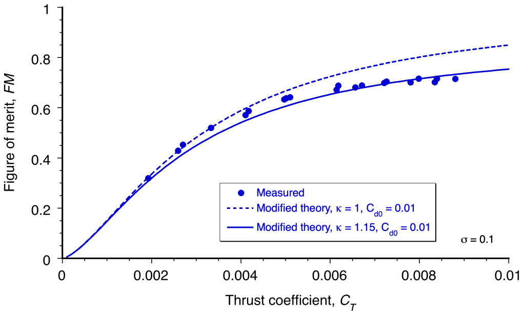
A representative plot of the measured figure of merit versus rotor thrust is shown below. It will be apparent that the  reaches a maximum and then remains constant or drops off slightly. This latter behavior results from the higher-profile drag coefficients (
 ) observed at higher rotor thrusts. For some rotors, especially those with less efficient airfoils, the curve can exhibit a peak in , followed by either a gradual or abrupt decrease thereafter. Therefore, the behavior in the high thrust range will, to some extent, be a function of the airfoils used on the blades and their stall type. In practice, maximum values between 0.65 and 0.75 represent a good hovering performance for a helicopter rotor.
The figure of merit for the best hovering efficiency can now be established, i.e., maximum power loading. The ratio of the power required to hover to the thrust produced is
(35) 
which can be written in terms of the modified momentum theory with the parameters and as
(36) 
The operating  to give the best power loading can be obtained by differentiating Eq. 36 with respect to , i.e.,
(37) 
which must be zero for a minimum. Therefore,
(38) 
which, on rearrangement, gives
(39) 
Substituting the result that  into the figure of merit expression gives
(40) 
 .
.For design purposes, solving for the rotor radius determines its optimal value for a given helicopter gross weight, rotor tip speed, and operational density altitude. However, in most cases, the resulting radius is too high to be practical, i.e., the rotor will be so oversized that it would be excessively heavy. Furthermore, the helicopter would not be able to fit into a hangar or be accommodated at an airfield otherwise. Therefore, the rotor must be operated at a higher disk loading than the optimum.
As shown in the figure below, the rotor’s efficiency is relatively insensitive to thrust at its most efficient operation, as the  curve is reasonably flat above a particular thrust coefficient. Therefore, there is some latitude when selecting the rotor radius, which may be constrained by factors other than aerodynamics.
Finally, a word of caution is appropriate regarding the figure of merit. To be meaningful, the figure of merit must only be used as a gauge of rotor efficiency when two or more rotors are compared at the same disk loading, which can be seen if the figure of merit is written dimensionally as
(41) 
Therefore, it would be inappropriate to compare the figures of merit of two rotors with different disk loadings because, with all other factors being equal, the rotor with the higher disk loading will generally always give the higher figure of merit.
Check Your Understanding #3 – Hovering power required
A tiltrotor has a gross weight of 45,000 lb (20,400 kg). The rotor diameter is 38 ft (11.58 m). Based on the momentum theory, estimate the power required for the aircraft to hover at sea level on a standard day out of ground effect where the density of air is 0.002378 slugs ft or 1.225 kg m. Assume that the figure of merit of the rotors is 0.75, and transmission losses amount to 5%.
Show solution/hide solution.
A tiltrotor has two rotors, each assumed to carry half the total aircraft weight, that is,  22,500 lb. Each rotor’s disk area is
  ft. The induced velocity in the plane of the rotor is
![\[ v_h = \sqrt{ \frac{T}{2 \varrho \, A} } = \sqrt{ \frac{22,500}{2 \times 0.002378 \times 1,134.12} } = 64.56~\mbox{ ft s$^{-1}$} \]](https://eaglepubs.erau.edu/app/uploads/quicklatex/quicklatex.com-ec9c67eb56a6142da6595208b4910e63_l3.svg "Rendered by QuickLaTeX.com")
The ideal power per rotor will be
![\[ P_{\rm ideal} = T v_h = 22,500 \times 64.56 = 1,452,600~\mbox{ft-lb s$^{-1}$} \]](https://eaglepubs.erau.edu/app/uploads/quicklatex/quicklatex.com-7ee9a71ffe6fa0275fa344563334143c_l3.svg "Rendered by QuickLaTeX.com")
This result is converted to horsepower (hp) by dividing by 550, yielding 2,641 hp per rotor. Remember that the figure of merit accounts for the aerodynamic efficiency of the rotors. Therefore, the actual power required per rotor to overcome induced and profile losses will be 2,641/0.75 = 3,521.5 hp. Multiplying this result by two to account for both rotors yields  7,043 hp. Transmission losses account for another 5%, so the total power required to hover is
  7,395 hp.
The problem can also be worked on in SI units. In this case,  100,062 N. The disk area is,
  m. The induced velocity in the plane of the rotor is
![\[ v_i = \sqrt{ \frac{T}{2 \varrho \, A} } = \sqrt{ \frac{100,062}{2 \times 1.225 \times 105.35} } = 19.69~\mbox{ m s$^{-1}$} \]](https://eaglepubs.erau.edu/app/uploads/quicklatex/quicklatex.com-d1824922e54648b7884005e1ca8dbbc4_l3.svg "Rendered by QuickLaTeX.com")
The ideal power per rotor will be
![\[ T v_h = 100,062 \times 19.69 = 1,970.2~\mbox{kW} \]](https://eaglepubs.erau.edu/app/uploads/quicklatex/quicklatex.com-8b59266467f9ebee5d55c3093e75d0af_l3.svg "Rendered by QuickLaTeX.com")
The actual power required per rotor to overcome induced and profile losses will be 1,970.2/0.75 = 2,626.9 kW. Multiplying this result by two to account for both rotors yields 5,253.8 kW. Transmission losses mean the total power required to hover will be 5,515.7 kW.
Solidity & Blade Loading Coefficient
It will be seen from Eq. 34 that the solidity, , appears in the expression for the figure of merit, . For a rotor with rectangular blades, the solidity represents the ratio of the lifting area of the blades to the area of the rotor, i.e.,
(42) 
As previously noted, typical values of range from about 0.05 to 0.15 for helicopters.
If is plotted for rotors with different values of , the behavior is typified by the figure below. While the number of blades also affects rotor performance, there are no known measurements of the effects of solidity independent of the number of blades. Results predicted using the modified momentum theory are also shown. From the measurements at zero thrust, it was deduced that  and that was about 1.25.
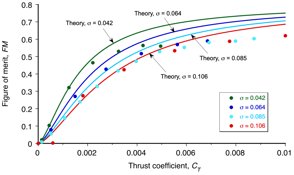
It will be noted that higher values of are obtained with the lowest possible solidity at the same design , i.e., same aircraft gross weight or disk loading. This result is hardly unexpected from Eq. 34, given that all other terms, such as , are assumed to be constant, meaning that the viscous drag on the rotor is minimized by reducing the net blade area. However, the minimization of must be done with caution because reducing the blade area must always result in a higher angle of attack of the blade sections (and higher lift coefficients) to obtain the same values of .
Therefore, the lowest allowable value of must ultimately be limited by the onset of blade stall. The results show this latter effect at the lowest solidity of 0.042, where a progressive departure from the theoretical predictions occurs for  . This behavior would occur at higher values of for a full-scale rotor because the blades exhibit higher maximum lift at higher Reynolds numbers.
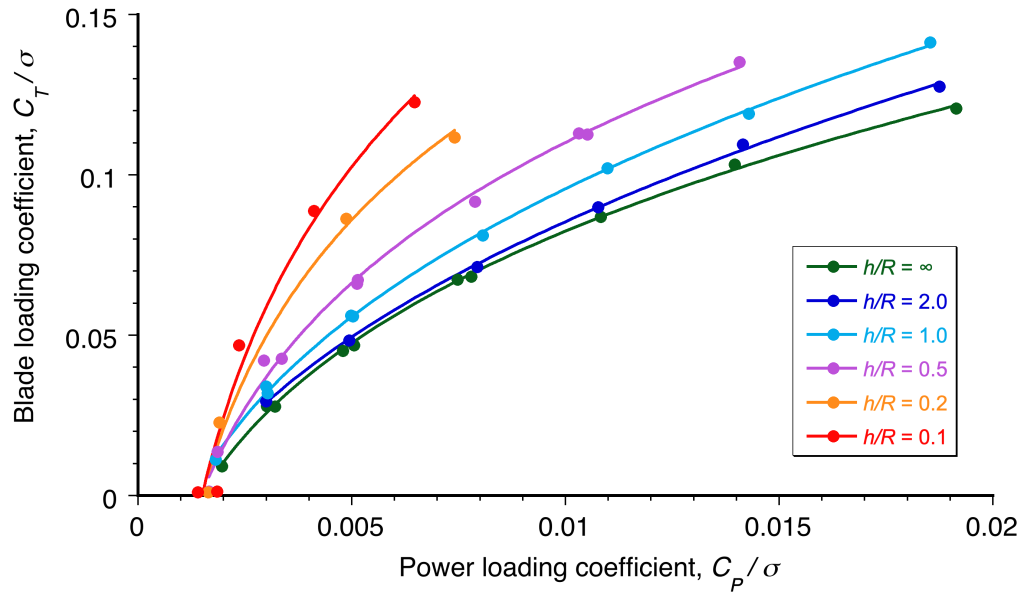
Therefore, an alternative presentation is to plot the figure of merit versus the blade-loading coefficient,  , as shown in the figure below. In this case, can be written as
(43) 
where  is the area of the blades.
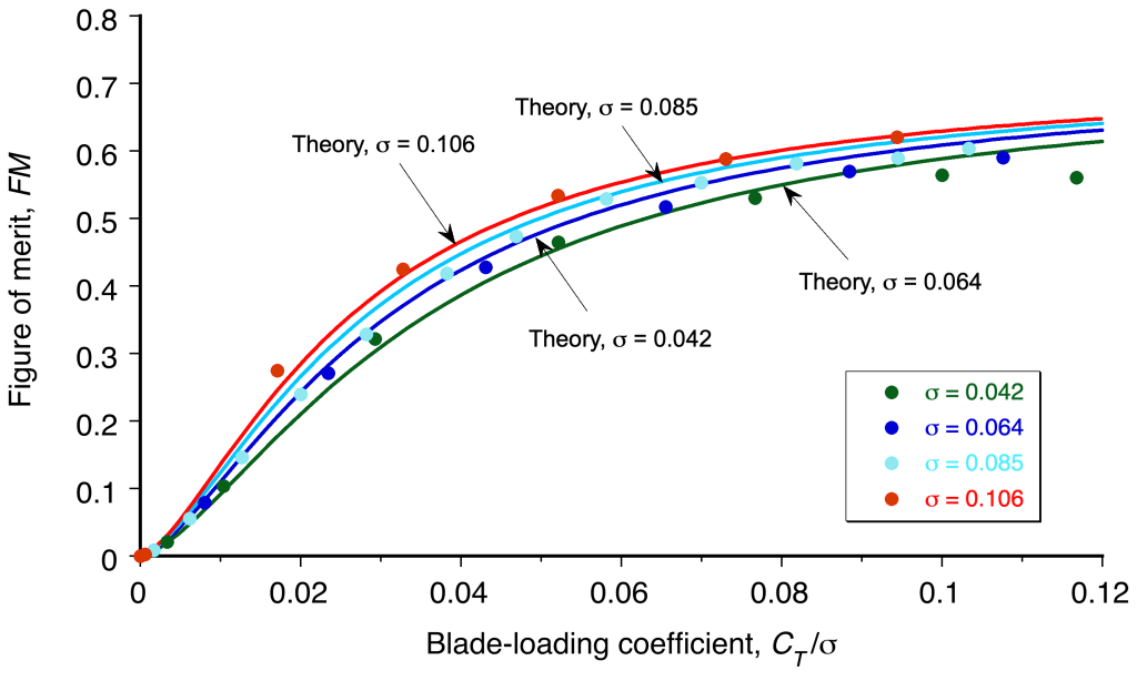
Notice that reducing the value of results in higher values of for the same value of . Although the rotor operates at higher values of with an increased blade loading coefficient, the maximum value is limited by the onset of blade stall. Typically, for a contemporary helicopter rotor, the maximum realizable value of the blade loading coefficient without stall is about 0.12 to 0.14. However, the influence of Reynolds number on blade stall must also be considered, especially with subscale rotors.
The maximum attainable value of will also depend on the distribution of local lift coefficients along the blade, which depends on both the blade twist and its planform shape. The local lift coefficients can be related to the blade loading using the blade element theory, so the blade twist and blade planform can be designed to delay the stall effects to higher values of . The blade element theory is described later in this chapter. A rotor with airfoils featuring higher maximum lift coefficients can also be designed with lower solidity. This approach offers the benefit of lower blade and hub weight, which significantly reduces total helicopter weight.
Ground Effect
Just like airplanes, helicopter performance is affected by the presence of the ground or any other boundary that may alter or constrain the flow into the rotor or constrain the development of the wake, as shown in the figure below. Because the ground must be a streamline to the flow, the rotor slipstream tends to expand rapidly as it approaches the ground. This behavior alters the slipstream velocity, the induced velocity in the rotor plane, and, therefore, the rotor thrust and power. Similar effects are obtained in hover and forward flight, but the effects are most substantial in the hovering state.
A representative set of power polars for a rotor hovering near the ground is shown in the figure below. The results suggest significant effects on hovering performance for heights less than one rotor diameter. When the hovering rotor operates in ground effect, its thrust increases for a given power input. Alternatively, this effect can be viewed as a reduction in power for a given thrust (weight). Remember that a straight line drawn from the point (0, 0) to any point on a polar curve gives the ratio of , or the power loading, which measures efficiency. Notice that efficiency is highest at the lowest rotor heights off the ground.
Check Your Understanding #4 – Induced power factor & profile power
A student measures the rotor performance at a fixed rotor speed for a series of blade pitch angles. The rotor has a solidity of 0.1. The values of the thrust coefficient, , that were measured were 6.0000E-06, 0.001049, 0.002375, 0.004075, and 0.005582, and the corresponding values of the power coefficient, , were 0.000196, 0.000225, 0.000281, 0.000404, and 0.000554, respectively. The student aims to estimate the rotor’s induced power factor, the zero-thrust (profile) power, and the mean section drag coefficient.
Show solution/hide solution.
The simple momentum theory gives the ideal power as
![\[ C_{P_{\rm ideal}} = \frac{C_T^{3/2}}{\sqrt{2}} \]](https://eaglepubs.erau.edu/app/uploads/quicklatex/quicklatex.com-6e11a7c01d860379575c8e081da861d7_l3.svg "Rendered by QuickLaTeX.com")
and the modified momentum theory is
![\[ C_{P_{\rm}} = \frac{\kappa \, C_T^{3/2}}{\sqrt{2}} + C_{P_{0}} \]](https://eaglepubs.erau.edu/app/uploads/quicklatex/quicklatex.com-f051b296067120a7b329468d51094c72_l3.svg "Rendered by QuickLaTeX.com")
The student wants to find values of and  so we can write
![\[ C_{P_{\rm}} = \kappa \, C_{P_{\rm ideal}} + C_{P_{0}} \]](https://eaglepubs.erau.edu/app/uploads/quicklatex/quicklatex.com-5fed0d7e3d8d5fd1ec8052fb6d756d79_l3.svg "Rendered by QuickLaTeX.com")
and so to find these values we can plot  versus
  , which should be close to a straight-line.
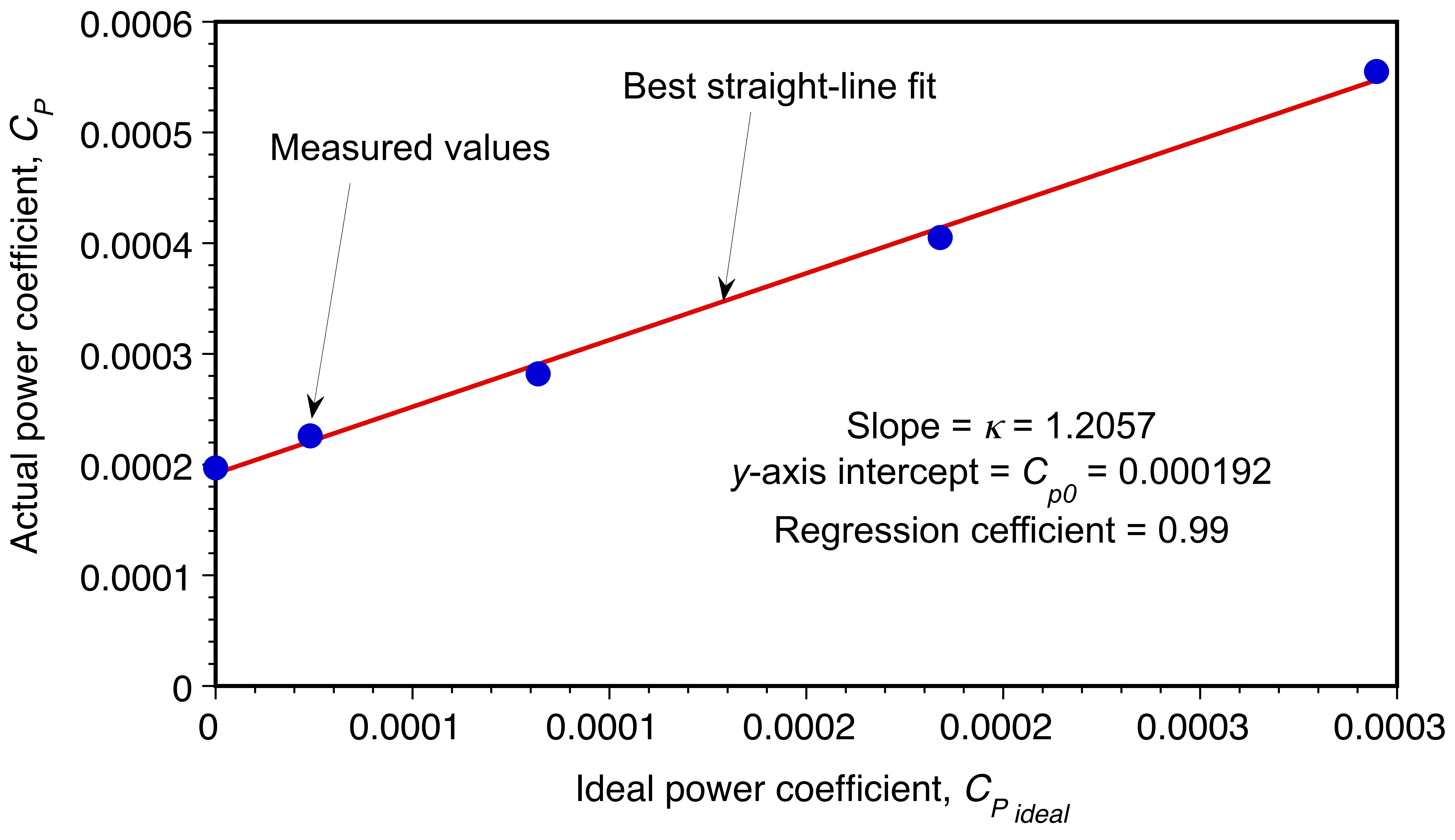 The best straight-line fit (least-squares) gives the slope , and the intercept on the -axis is . In this case the value of is 1.206 and is 0.000192. It is then possible to estimate the average drag coefficient of the airfoils that comprise the rotor using
![\[ C_{P_{0}} = \frac{\sigma \, C_{d_{0}}}{8} \]](https://eaglepubs.erau.edu/app/uploads/quicklatex/quicklatex.com-b969be84b741f82b83c8811ad8559285_l3.svg "Rendered by QuickLaTeX.com")
so
![\[ C_{d_{0}} = \frac{8 C_{P_{0}}}{\sigma} \]](https://eaglepubs.erau.edu/app/uploads/quicklatex/quicklatex.com-06b29bb09e9298167aee1832616044cc_l3.svg "Rendered by QuickLaTeX.com")
If  as stated, then
  , which seems fairly reasonable.
Axial Climbing & Descending Flight
Adequate climbing flight performance is an essential operational consideration for a helicopter, and sufficient power reserves must be available to ensure it over a wide range of flight weights and operational density altitudes. Increasing altitude takes more power than losing altitude. Estimates of the power required for climbing and descending can also be obtained through a momentum-based analysis.
Climbing Flight
The three conservation laws are applied to a control volume surrounding the climbing rotor and its flow field, as shown in the figure below. As before, consider the problem one-dimensional, and assume the flow properties vary only in the vertical direction across cross-sectional planes parallel to the disk. At each cross-section, the flow properties are distributed uniformly.
In contrast to the hover case, where the climb velocity is identically zero, the relative velocity far upstream relative to the rotor will now be  . At the plane of the rotor, the velocity will now be
  , and the slipstream velocity is now
  .
.
The mass flow rate is constant within the slipstream boundary and can be defined at the rotor, i.e.,
(44) 
The thrust on the rotor, in this case, will be
(45) 
Notice that this is the same equation for the rotor thrust as in the hover case, i.e., Eq. 4.
Because the work done by the climbing rotor is  , then
(46) 
From Eqs. 45 and 46 it is readily apparent that .
The relationship between the rotor thrust and the induced velocity at the rotor disk in hover is
(47) 
and for the climbing rotor using Eq. 45, then
(48) 
so that
(49) 
which is a quadratic equation in . Dividing through by  to make it non-dimensional gives
(50) 
which is a quadratic equation in  . This equation has a solution
(51) 
Although there are two possible solutions (positive and negative), must always be positive in the climb to avoid violating the assumed flow model. The valid solution is
(52) 
Descending Flight
The climb flow model cannot be used in a descent (where  ) because is now directed upward so that the slipstream will be above the rotor. This will be the case whenever
  is more than twice the average induced velocity at the disk. For cases where the descent velocity is in the range
  , the velocity at any plane through the rotor slipstream can be upward or downward. Under these circumstances, a definitive control volume surrounding the rotor and its wake cannot be established.
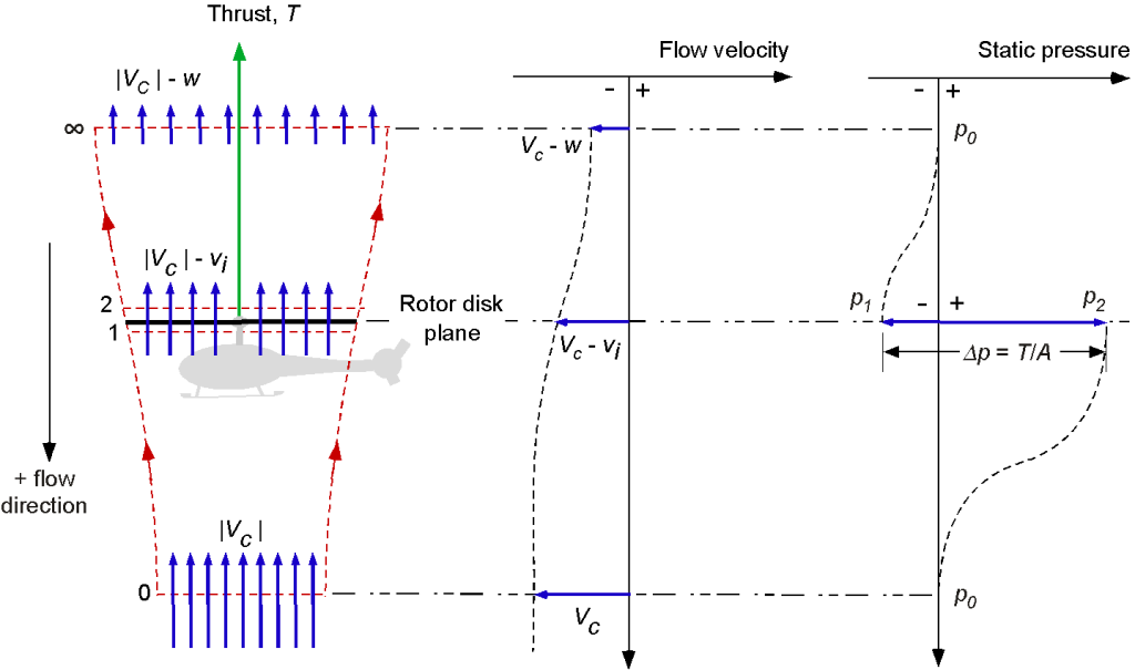
The assumed flow model and control volume surrounding the descending rotor are shown in the figure below. To proceed, the assumption must be made that  so that a well-defined slipstream will always exist above the rotor and encompass the limits of the rotor disk. Far upstream (well below) the rotor, the magnitude of the velocity is the descent velocity, which is equal to . Notice that to avoid ambiguity, it will be assumed that the velocity is measured as positive when directed downward. At the plane of the rotor, the velocity is
  . In the far wake (above the rotor), the velocity is
  .
.
The mass flow rate, , through the rotor disk is
(53) 
The thrust, in this case, can be expressed as
(54) 
Notice that is not negative because is negative using the assumed sign convention.
(55) 
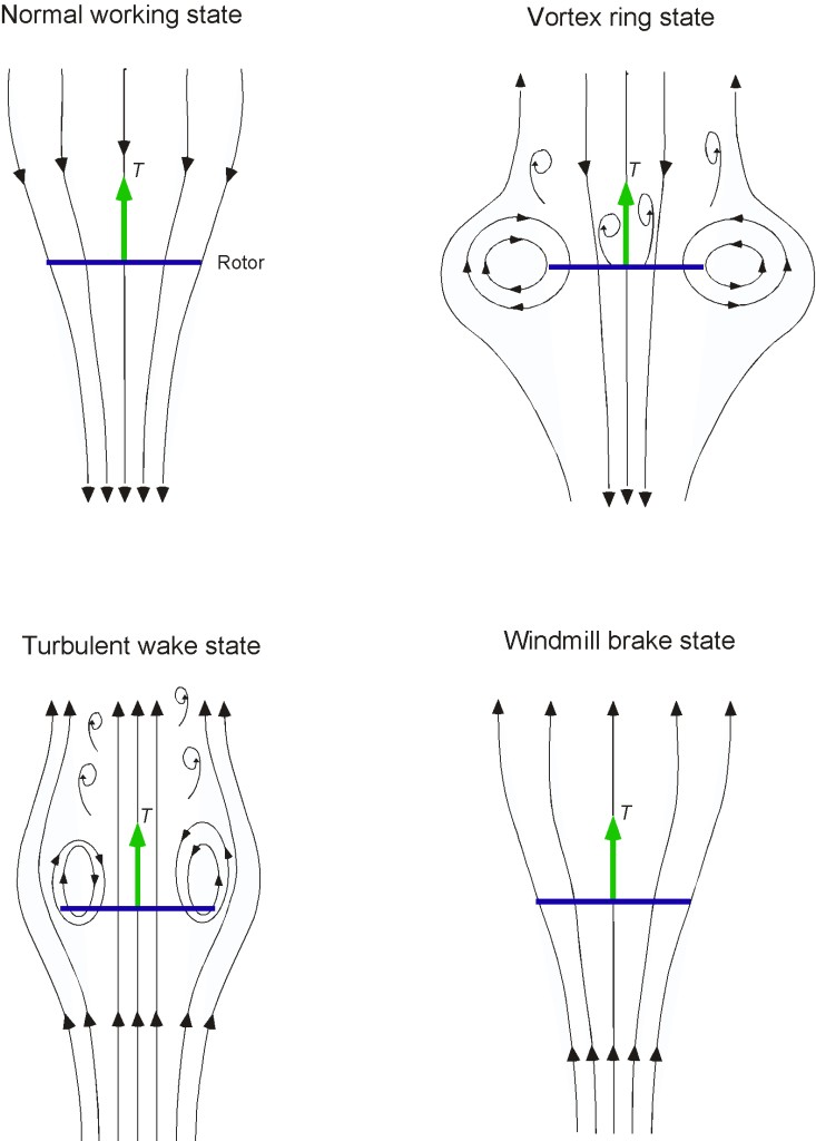
which is a negative quantity. Therefore, the rotor must extract power from the airstream, and this operating condition is known as the windmill state. It is usually referred to as the windmill brake state because, in this condition, the rotor decreases or “brakes” the flow velocity.
Using Eqs. 54 and 55 it is seen, again, that . Note, however, that the net velocity in the slipstream is less than , so from continuity considerations, the wake boundary expands above the descending rotor disk. For the descending rotor, then
(56) 
so that
(57) 
Dividing through by gives
(58) 
which is a quadratic equation in . This equation has a solution
(59) 
Again, as in the climb case, two possible solutions for during descent exist. The only valid solution is
(60) 
which is applicable for  .
.
Induced Velocity Curves
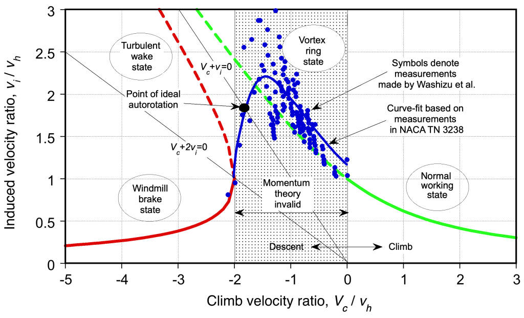
The results from the preceding analysis are presented below. It is apparent that as the climb velocity increases, the induced velocity at the rotor decreases. This condition is the normal working state of the rotor, with hover as the lower limit. The branch of the induced velocity curve denoted by the broken line gives a solution to Eq. 52 for negative values of , i.e., a descent. However, as the rotor begins to descend, there are two possible flow directions, one of which violates the assumed flow model; therefore, this solution is physically invalid. This condition, called the Vortex Ring State (VRS), can be described only from measurements.
Power Required Curves
Because both climb and descent change the induced velocity at the rotor, the induced power will be affected accordingly. The power ratio can be written as
(61) 
where the first term is the useful work to change the potential energy of the rotor (helicopter), and the second term is the work done on the air by the rotor, i.e., the irrecoverable induced losses.
Using Eq. 52 and substituting and rearranging gives the power ratio for a climb as
(62) 
In a descent, Eq. 60 is applicable. Substituting this into Eq. 61 and rearranging gives the power ratio as
(63) 
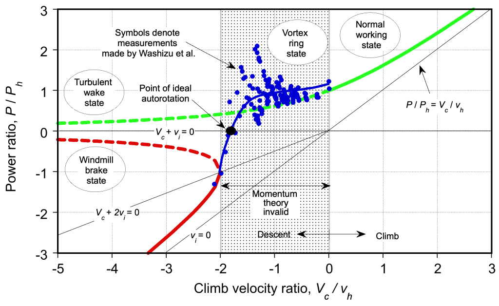
The figure below shows the total rotor power ratio,  , plotted versus the climb ratio,
  . The power required to climb is always greater than that needed to hover. However, as the climb velocity increases, the induced power becomes a progressively smaller percentage of the total power required to climb. It is also significant to note that, in descent, at least above a specific rate, the rotor extracts power from the air and uses less power than required to hover; i.e., it operates like a windmill. However, a helicopter rotor will never operate in this condition.
Vortex Ring State
In the region  , called the vortex ring state (VRS), the momentum theory is invalid because the flow can take on two possible directions, and a well-defined slipstream ceases to exist, as shown in the figure below. In the VRS, the rotor can experience highly unsteady flow with regions of concurrent upward and downward velocities, and the flow can periodically break away from the rotor disk. This means a control volume encompassing only the rotor disk’s physical limits cannot be defined. From a piloting perspective, VRS is not a sustainable flight condition. Unsteady flow at the rotor in VRS can lead to a loss of rotor control. If the VRS occurs on the tail rotor, such as during a sideslip or while hovering in a crosswind, then directional (yaw) control may be seriously impaired.
The induced velocity curve in the VRS can still be defined empirically, albeit only approximately, based on rotor experiments. Even then, measuring rotor thrust and power is difficult. The average induced velocity is then obtained indirectly from the measured rotor power and thrust using the assumed form
(64) 
where is the profile power, and where  is recognized as only an averaged value of the induced velocity through the disk. Using the result that
  then
then
(65) 
Therefore, in addition to the measured rotor power  , it is necessary to know the rotor profile power to estimate the averaged induced velocity ratio. As shown previously using Eq. 30, a straightforward estimate for the profile power coefficient of a rotor with rectangular blades is
  . Because of the high levels of turbulence near the rotor in the VRS, the derived measurements of the average induced velocity exhibit a relatively large amount of scatter.
These measurements can then be used to find a “best-fit” approximation for at any rate of descent. One approximation is
(66) ![\begin{equation*} \frac{v_i}{v_h} = \left\{\begin{array}{ll} 1 - \displaystyle{\frac{V_c}{v_h}} & \mbox{~~for~} -1.5 \le \displaystyle{\frac{V_c}{v_h}} \le 0 \\[20pt] 7 + 3 \displaystyle{\frac{V_c}{v_h}} & \mbox{~~for~} -2 \le\displaystyle{\frac{V_c}{v_h}} \le -1.5\end{array} \right. \end{equation*}](https://eaglepubs.erau.edu/app/uploads/quicklatex/quicklatex.com-5ebb2df9f6e9a765c173d21e853d25af_l3.svg "Rendered by QuickLaTeX.com")
Autorotation in Vertical Flight
The principle of autorotation can be observed in nature, as seen in the flight of sycamore or maple seeds, which spin rapidly as they slowly descend and are often carried on the wind for considerable distances. An autorotation is a maneuver that can be used to recover the helicopter to the ground in the event of an engine failure, transmission problems, or loss of the tail rotor. It requires that the pilot let the helicopter descend at a sufficiently high but controlled rate, where the energy to drive the rotor can be obtained by giving up potential energy (altitude) for kinetic energy taken from the relative upward flow through the rotor, thereby averting a ballistic fall.
Notice that from the power curve shown previously, there is a value of for which zero net power is required for the rotor, i.e.,  or
or  . This condition is called ideal autorotation for vertical flight. It is a self-sustaining operating state in which the energy to drive the rotor comes from potential energy converted to kinetic energy from the relative descent velocity (upward relative to the rotor). Based on assuming the validity of Eq. 66, it will be apparent that the power curve crosses the ideal autorotation line
  at
at
(67) 
which gives  for an ideal rotor (
 ). In practice, a real (actual) autorotation in axial flight occurs at a slightly higher rate than this because, in addition to induced losses at the rotor, there is also a proportion of profile losses to overcome. In a real autorotation, then
(68) 
Therefore, in a stable autorotation, an energy balance must exist where the decrease in potential energy of the rotor  balances the sum of the induced
  and profile
  losses of the rotor. Using Eq. 68, this condition is achieved in vertical descent when
(69) 
which depends primarily on the disk loading. Also, using the definition of figure of merit (and assuming the induced and profile losses do not vary substantially from the hover values), then
(70) 
Using Eq. 66 for the induced velocity with Eq. 70 gives the real autorotation condition
(71) 
The first term on the right-hand side of Eq. 71 will vary in magnitude from  to
to  , depending on the rotor efficiency. Compared to the second term, the extra rate of descent required to overcome profile losses is relatively small. Therefore, based on the preceding, it is apparent that a real vertical autorotation will occur for values of between
  and
and  .
.
It is found that autorotations must be performed at relatively high descent rates with a helicopter. Using the result that  , where is in lb/ft, gives
  ft s for autorotation at sea level conditions, which for a representative disk loading of 10 lb ft leads to a vertical rate of descent of about 5,000 ft min. However, as discussed later in this chapter, with forward speed, the power required at the rotor is considerably lower than in the hover case.
Check Your Understanding #5 – Climb power required
A helicopter weighing 6,000 lb is required to hover and climb vertically at 600 ft/min. The main rotor’s radius is 20 ft, and its figure of merit is 0.75. Determine the power required. Assume sea level conditions. Discuss the factors that will determine a helicopter’s maximum vertical climb rate.
Show solution/hide solution.
The power required in an axial climb can be estimated from the momentum theory result that
![\[ \frac{P}{P_h} = \frac{V_c}{2v_h} + \sqrt{ \left( \frac{V_c}{2 v_h}\right)^2 +1 } \approx \frac{V_c}{2v_h} + 1 \mbox{~~for low to moderate climb rates.} \label{powerclimb3} \]](https://eaglepubs.erau.edu/app/uploads/quicklatex/quicklatex.com-35c08d8de262c8660e492a5b81853510_l3.svg "Rendered by QuickLaTeX.com")
In hover, the induced velocity, , is
![\[ v_h = \sqrt{ \frac{T}{2 \varrho \, A} } = \sqrt{ \frac{ 6,000}{2 \times 0.00238 \times \pi \times (20.0)^2 }} = 31.67~\mbox{ft/s} \]](https://eaglepubs.erau.edu/app/uploads/quicklatex/quicklatex.com-a6b2e7d24dad133f3be5feba48db8c3c_l3.svg "Rendered by QuickLaTeX.com")
where at sea level conditions  slugs/ft
 . The power required to hover will be
![\[ P_h = (1/0.75) \frac{T^{3/2}}{\sqrt{ 2 \varrho \, A}} = \frac{ 1.333 \times (6,000)^{3/2}}{\sqrt{2 \times 0.00238 \times \pi \times (20.0)^2 }} \times \frac{1}{550} = 460.66~\mbox{hp} \]](https://eaglepubs.erau.edu/app/uploads/quicklatex/quicklatex.com-2e308f48491b585779519c24554343c2_l3.svg "Rendered by QuickLaTeX.com")
The power required to climb at 600 ft/min (10 ft/s) will be
![\[ P \approx P_h \left( \frac{V_c}{2 v_h} + 1 \right) = 460.66 \left( \frac{10.0}{2 \times 31.67} + 1 \right) = 533.49~\mbox{hp} \]](https://eaglepubs.erau.edu/app/uploads/quicklatex/quicklatex.com-755134fa622914ef82bbd0dc0f25917a_l3.svg "Rendered by QuickLaTeX.com")
The maximum rate of climb of the helicopter will be determined by the excess power available over and above that required to hover at the same weight and density altitude. The vertical drag produced on the airframe may also be a factor in the climb condition, albeit at high climb rates.
Hovering Coaxial Rotor
The recent interest in coaxial rotor systems has been driven by advancements in electric propulsion, urban air mobility (UAM), and the development of high-speed vertical takeoff and landing (VTOL) aircraft for military applications. Coaxial rotors offer a helicopter a smaller footprint, making them ideal for eVTOL air taxis and uncrewed aerial vehicles (UAVs). Still, this advantage comes at a price, including significantly lower aerodynamic efficiency for a given net thrust, i.e., higher power requirements. The main reason is that the lower rotor operates in the upper rotor’s wake, thereby incurring higher aerodynamic losses.
There are not one but four primary cases of interest for a coaxial rotor system: 1. The two rotors corotate in the same plane (or very nearly so in practice) and are operated at the same individual values of thrust; 2. The two rotors corotate in the same plane at different thrusts but are operated at a balanced (equal and opposite) torque; 3. The rotors are operated at the same individual thrust values, but the lower rotor operates in the fully developed slipstream, i.e., in the fully contracted wake of the upper rotor; 4. The rotors are operated at balanced torque, with the lower rotor operating in the fully contracted wake of the upper rotor. Solutions for each of these operating cases can be derived using the momentum theory.
Corotation in the Same Plane
Suppose the two rotors of a coaxial rotorcraft rotate in the same plane of rotation. In that case, they can be operated at the same individual thrust values or at balanced torque; the latter is more practical. The momentum theory can analyze both conditions.
Equal Thrusts
Assume first that the distance between the rotor planes is infinitesimally small, as shown in the figure below, such that they share the same induced velocity  and that each rotor of the system provides an equal fraction of the total system thrust (i.e.,
  ) where
  . The effective induced velocity of the rotor system will be
(72) 
where is the disk area of any one rotor. Therefore, the induced power of the system,  , is
, is
(73) 
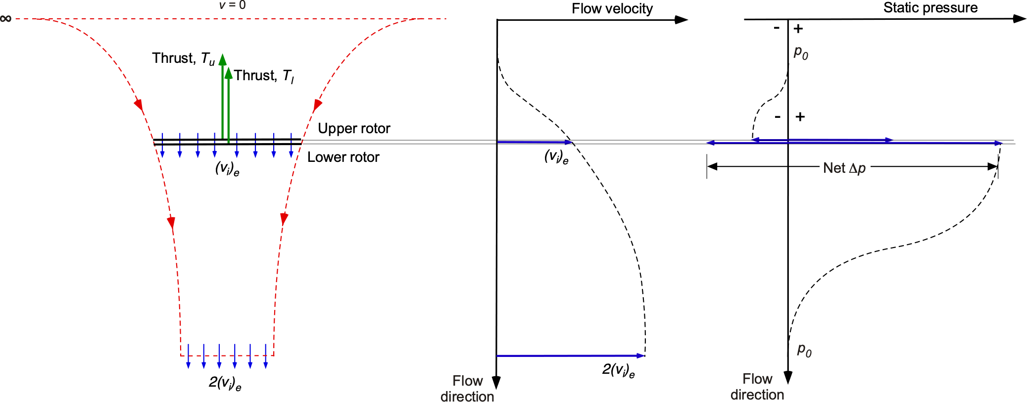
One way to compare coaxial rotor performance levels is to treat each rotor as an entirely free, isolated rotor. This is equivalent to comparing the coaxial rotor to two single, isolated rotors operating at the same disk loading as either rotor of the coaxial rotor. The main point is to compare rotor performance levels under the same disk loading to avoid biasing the results.
The induced power for either isolated rotor will be  (the upper rotor is equivalent to the isolated rotor because its performance is assumed to be unaffected by the lower rotor), and so for the two separate rotors, the total induced power is
(74) 
The interference-induced power factor  for the coaxial rotor system can then be defined as the ratio of the results in Eqs. 73 and 74, giving
(75) 
In this case, there is a 41% increase in the induced power required relative to the power required to operate the same two rotors of the system separately in complete isolation. This is a significant performance loss. The net ideal induced power of the coaxial rotor system can, therefore, be written simply as
(76) 
Notice that two single rotors, each of area and each carrying a thrust , are equivalent to one single rotor of thrust  and of twice the disk area, i.e., one single rotor with its radius increased by a factor
  and with the same disk loading . Of course, in practice, such an equivalent single rotor must have the same net solidity as the coaxial rotor for any equivalence to be considered valid. Furthermore, notice that the wake area contraction for the coaxial rotor under these assumptions is
  , the same as the contraction for a single rotor.
Balanced Torques
In practice, the two rotors of the coaxial rotor system are operated at individual thrust levels necessary to produce zero net torque; that is, they must be operated at equal and opposite torque levels. However, if the two rotors are sufficiently close that they co-rotate in substantially the same plane at the same thrust, they must also require the same torque. This is because both rotors share the same value of induced velocity (i.e., Eq. 72). It is, therefore, easily shown that for the upper rotor, the induced power required is
(77) 
And for the lower rotor, the induced power required is
(78) 
so that  . This means that for this second case of a coaxial rotor system with the rotors in the same plane operated at the same torque,
  , as found previously. Furthermore, when the rotors operate in the same plane, torque balance can be achieved only if
  ; any other thrust-sharing arrangement will disrupt it.
Lower Rotor in the Slipstream of the Upper Rotor
The foregoing momentum analysis of the coaxial rotor problem is overly pessimistic compared to measurements on coaxial rotors. One often-cited reason for the overprediction of induced power is the actual (finite) spacing between the two rotor planes. Generally, in practical coaxial designs, the rotors are spaced sufficiently far apart to prevent inter-rotor blade collisions from blade flapping, allowing the lower rotor to typically operate in the fully contracted wake of the upper rotor. This is supported by Taylor’s flow visualization results, shown in the photograph below, where the wake contracts quickly below the upper rotor and is fully contracted when the lower rotor ingests it.
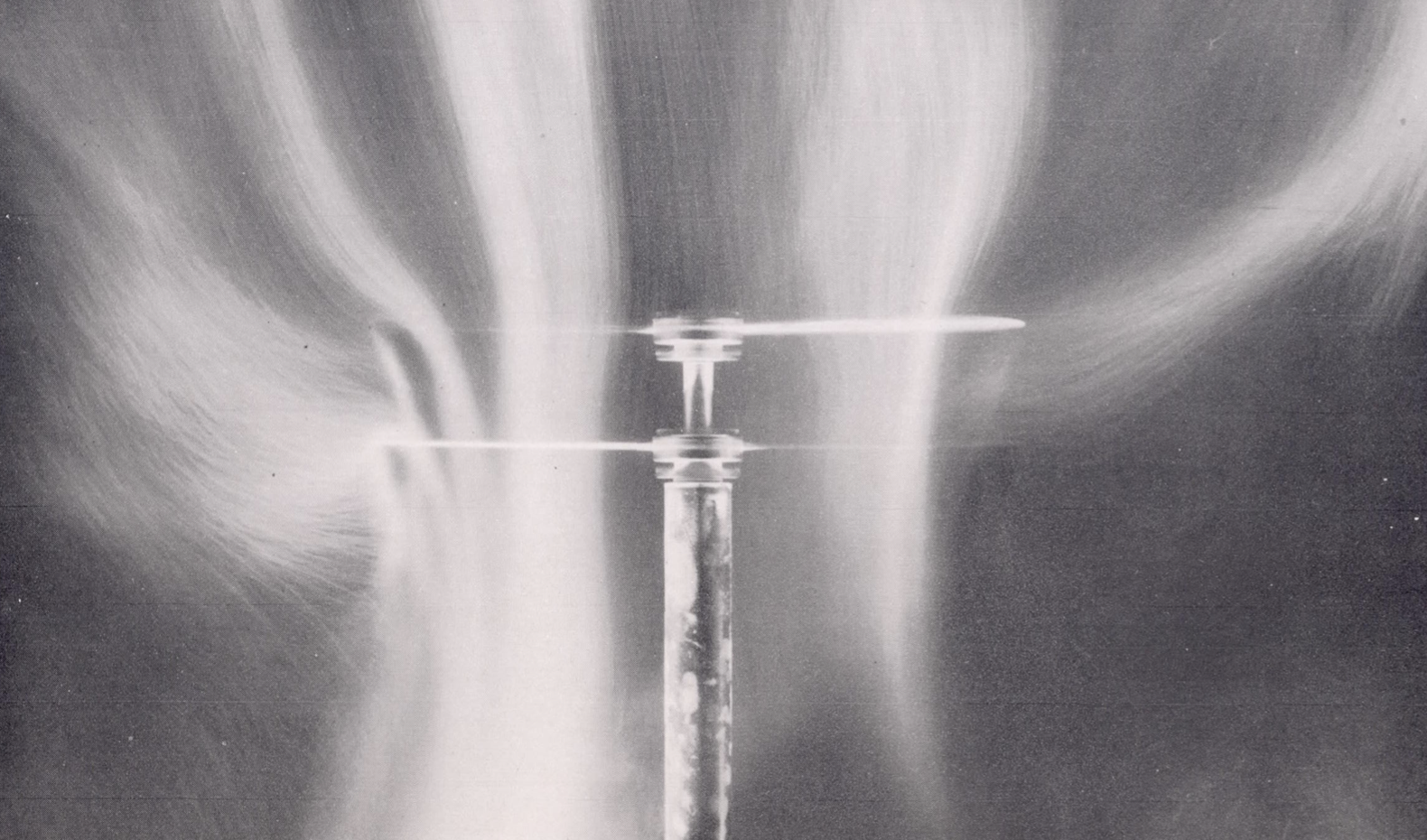
Proceeding by assuming that there is no non-ideal wake contraction and that the lower rotor does not affect the inflow, performance, or wake contraction of the upper rotor,[3] then the inner one-half of the disk area of the lower rotor must operate in the slipstream velocity induced by the upper rotor. This situation is, in general, a more complicated physical problem to model because it involves wake-blade interactions and local viscous effects at the wake boundary. However, the solution can be approached by following the same principles and assumptions as those made with the classic momentum theory.
Equal Thrusts
The flow model for this alternative situation is shown in the figure below. Assume first that the two rotors operate at the same thrust values, i.e.,  . The induced velocity at the upper rotor is
(79) 
The fully contracted wake produced by the upper rotor has an area of  and a slipstream velocity of
  . This represents the ideal case, although in practice, the wake contraction may not be as significant. Nevertheless, the ideal case is the tiniest fraction of the disk area on the lower rotor affected by the upper rotor, so it must represent the minimum induced-loss condition. Therefore, at the plane of the lower rotor, there is a velocity of
  over the inner one-half of the disk area. Over the outer one-half of the disk area, the induced velocity is
  . Assume that the velocity in the fully developed slipstream of the lower rotor (plane 3) is uniform with velocity
  .
.
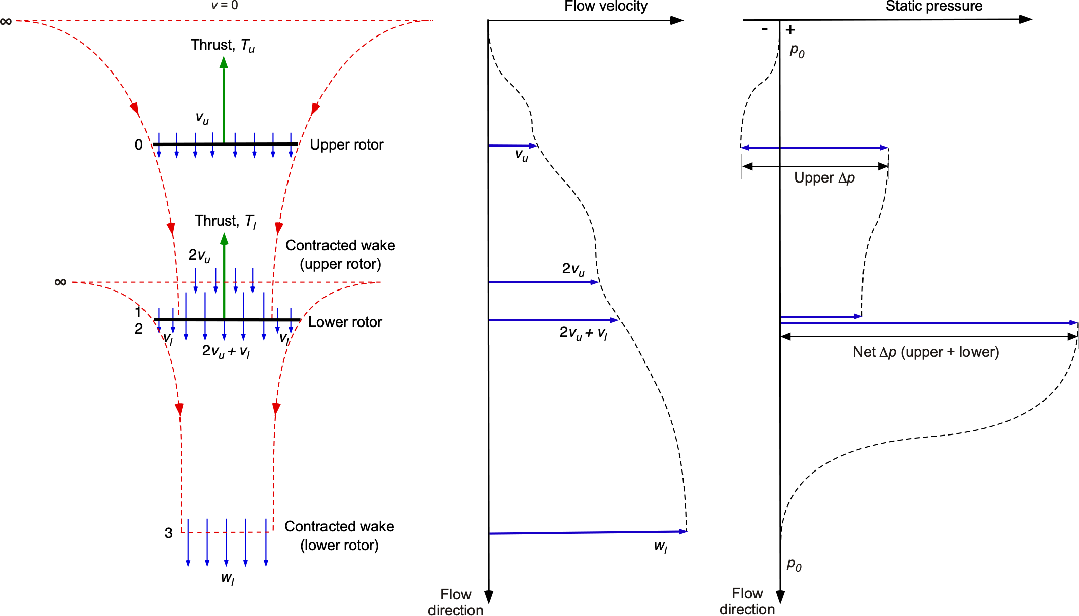
The mass flow rate of air through the upper rotor is  , so the momentum flux exiting in the slipstream of the upper rotor is
  . This is the momentum flux of the air entering the lower rotor. The mass flow rates over the inner and outer parts of the lower rotor are
  and
and  , respectively. Therefore, the total mass flow rate through the lower rotor, , is
(80) 
The momentum flux out of plane 3 is  , assuming uniform velocity, so the thrust on the lower rotor is
(81) 
The work per unit time done on the air by the lower rotor is
(82) 
This is equal to the gain in kinetic energy of the air in the slipstream. Therefore, expanding out gives
(83) 
Assuming equal thrusts on the upper and lower rotors (i.e.,  ), then
  . From Eq. 81
(84) 
and from Eq. 83 then
(85) 
Using Eqs.~84 and 85 gives  and substituting this into Eq. 84 and remembering that
  gives
gives
(86) 
Rearranging this latter equation as a quadratic in terms of and solving gives
(87) 
The interference-induced power factor can now be evaluated for this case. The power for the upper rotor is  , and for the lower rotor,
  . Therefore, the sum of the powers of both rotors is
  . This is compared to
  when the rotors operate in isolation.[4] This means that the interference-induced power factor, , is given by
(88) 
This now represents a 28.1% increase in the induced losses compared to a 41% increase when the two rotor disk planes have no vertical separation, i.e., in this case, = 1.2808. Such a result is much closer to the values that can be indirectly deduced from most experiments; see, for example, the coaxial rotor measurements of Harrington (hover) and Dingeldein (forward flight).
In this case, the wake area contraction differs for the single rotor and the coaxial rotors that co-rotate in the same plane. The wake area can be found from the continuity of the flows between the lower rotor and the far downstream wake, i.e.,
(89) 
which means the far downstream wake will contract less than for a single rotor.
Balanced Torques
A comparison of performance based on equal torque between the upper and lower rotors is a much more realistic operational assumption for a coaxial rotor. In this case, two solutions are of interest, differing in how they evaluate the interference-induced power factor. From the results of Eq. 81 and Eq. 83, with a torque balance such that  (i.e., equal rotor rotational and tip speeds), then
(90) 
Multiplying Eq. 81 by  and rearranging gives
(91) 
Now,  at the torque balanced condition, and using Eqs.~82 and 83 leads to
(92) 
Substituting Eq. 92 into Eq. 91 and rearranging gives
(93) 
Again, and substituting Eq. 93 in Eq. 82 gives
(94) 
which, on rearrangement, leads to
(95) 
Solving this cubic numerically leads to  . Again, notice that the area contraction of the far downstream wake is different from the prior cases, in this case being
(96) 
In this case, the interference-induced power factor can now be evaluated by considering the performance of the two isolated rotors (or equivalent single rotors at the same disk loading) when they are operated independently at equal thrust, as previously done. For a torque balance, then
(97) 
The thrust-sharing ratio is then
(98) 
As before, the interference-induced power factor is written as
(99) 
where the basis of comparison is with two isolated rotors operating at equal thrusts 
Now  at the torque balance, and also
  and
and  = 1.4375, so that
(100) 
An alternative basis for comparison with the coaxial rotor system is to use the performance of the two rotors (or an equivalent single rotor) when operated independently, but at the same thrust-sharing ratio as in the torque-balanced case. The interference-induced power factor in this situation is
(101) 
Again, at the torque balance, so in this case
(102) ![\begin{eqnarray*} \kappa_{\rm int} & = & \frac{2 P_u}{\displaystyle{\frac{T_u^{3/2}}{\sqrt{2 \varrho \, A}} + \frac{T_l^{3/2}}{\sqrt{2 \varrho \, A}}}} = \frac{2 T_u^{3/2}}{T_u^{3/2} + T_l^{3/2}} \nonumber \\[10pt] & = & \frac{2 \displaystyle{\left( \frac{T_u}{T_l}\right)^{3/2}}}{\displaystyle{\left(\frac{T_u}{T_l}\right)^{3/2}} + 1 } = 1.2657 \end{eqnarray*}](https://eaglepubs.erau.edu/app/uploads/quicklatex/quicklatex.com-67cb7711986732458994ed43c78fbe69_l3.svg "Rendered by QuickLaTeX.com")
This means that, for the assumptions made in this (final) case, the interference-induced power factor is 1.2657, which is slightly smaller than the value obtained when comparing two isolated rotors operating at equal thrusts or an equivalent single rotor with equal disk loading.
Remember that the foregoing results present the absolute minimum induced losses for each coaxial configuration under the stated assumptions and serve as a baseline for comparison with any real coaxial rotor system regarding operating efficiency.
Validity of the Coaxial Theory
Measurements, in this case, of a hovering coaxial rotor can establish the validity of the rotor momentum theory. The importance of the hovering condition cannot be overstated, as a rotor with poor hovering performance will likely underperform in forward flight and throughout the flight envelope.
There are very few measurements of coaxial rotor performance, but Harrington conducted performance measurements on two nominally full-scale sets of corotating coaxial rotors operating in hovering conditions. Both rotors had a diameter of 25 ft (7.62 m) and untwisted blades. Rotor 1 had two blades per rotor that were tapered in planform (approximately a 3:1 taper ratio) and corresponding thickness, with a thrust-weighted solidity of 0.027 (i.e., 2 0.054 when operated as a coaxial). Rotor 2 had two blades per rotor that were tapered only in the thickness-to-chord ratio, with a solidity of 0.076 (i.e., 2 0.152 as a coaxial rotor). Rotor 1 had an inter-rotor plane spacing of 0.186, and Rotor 2 had a rotor spacing of 0.16. Both sets of rotors were operated at a torque balance.
In summary, the theoretical power coefficient for the single-rotor system can be calculated using
(103) 
The corresponding power coefficient for the coaxial rotor system can be calculated using
(104) 
where represents the rotor-on-rotor induced power interference.
The two figures below show the results for the Harrington Rotor 1 and Rotor 2. It can be seen from the results that average values of = 1.1 for the Harrington 1 rotor and = 1.2 for the Harrington 2 rotor with = 1.280 in each case (Eqs. 103 and 104) give reasonably good overall agreement with the measurements of the power polars. Because the upper rotor generally operates at a higher thrust than the lower rotor to achieve a torque balance, the assumption that  = 1.2 gives a slightly better agreement with measurements than an assumption of balanced thrusts.
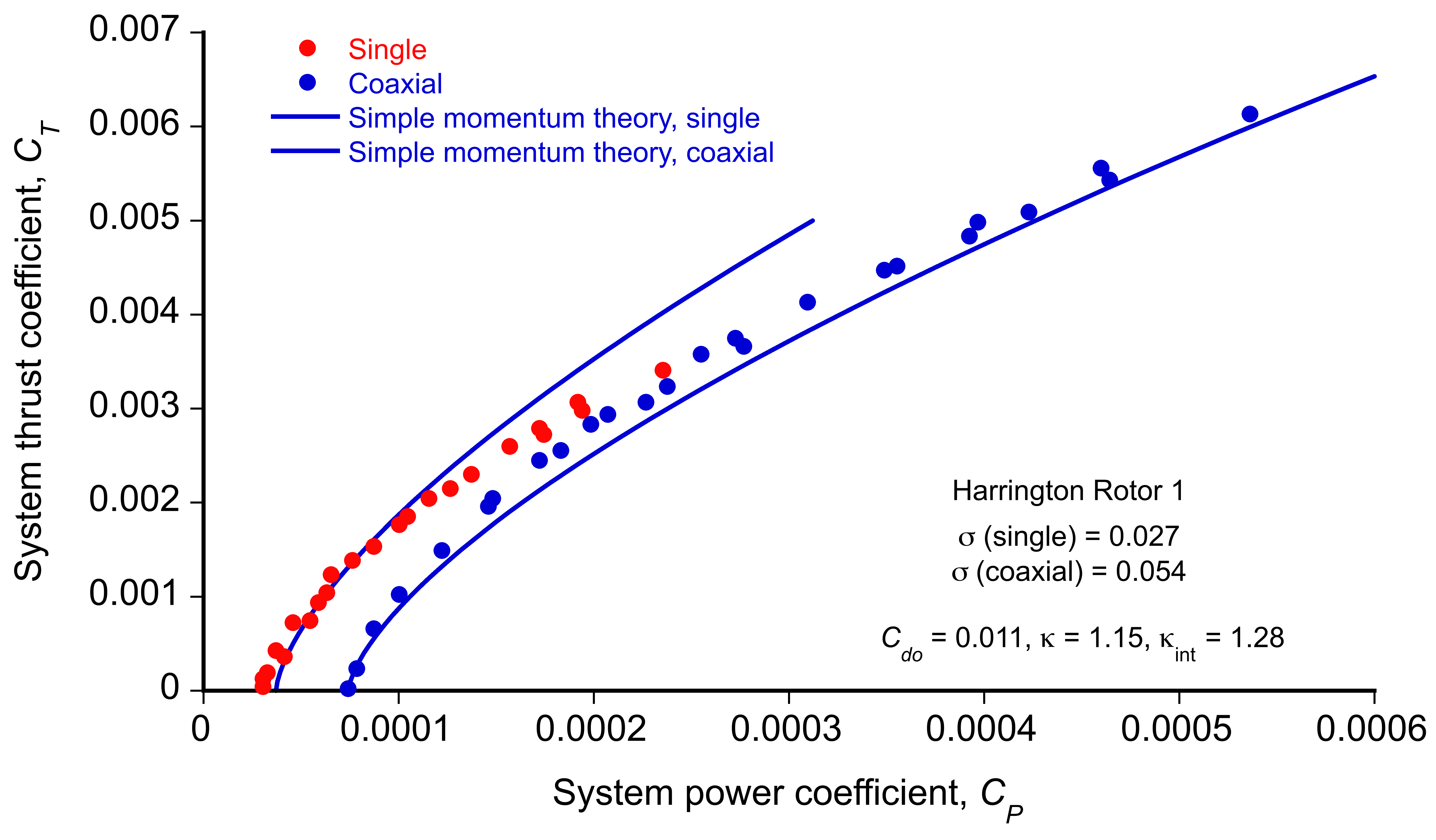
Notice that the inferred value of of 1.28 is just slightly larger than the minimum theoretical value of the interference-induced power factor with the lower rotor operating in the fully developed slipstream of the upper rotor, i.e., = 1.2657. Overall, these results confirm that the coaxial rotor behaves essentially as two isolated single rotors operating with the same disk loading as either of the upper or lower coaxial rotors, and with an induced interference effect between the rotors accounted for by an average induced power interference factor .
While it will be seen from the results that the agreement between predictions and experiment[5] are not uniformly good over all the operating conditions of the two sets of rotors. However, the momentum theory still gives a rational basis for analysis and a good benchmark for predicting coaxial rotor performance over some operational thrust ranges. Part of the underprediction of power stems from the assumption that the lower rotor does not affect the upper rotor, leading to a slight increase in the upper rotor’s power requirements. The values of both and depend on the rotor thrust, and the power required by the upper rotor depends on the lower rotor, helping to resolve the remaining differences observed here using the momentum theory. The under-prediction of power for the coaxial most likely arises from viscous interactions between the upper and lower rotors. Nevertheless, the intrinsic value of the momentum theory is evident in its continued ability to provide insight into the primary performance characteristics of both single- and coaxial-rotor systems.
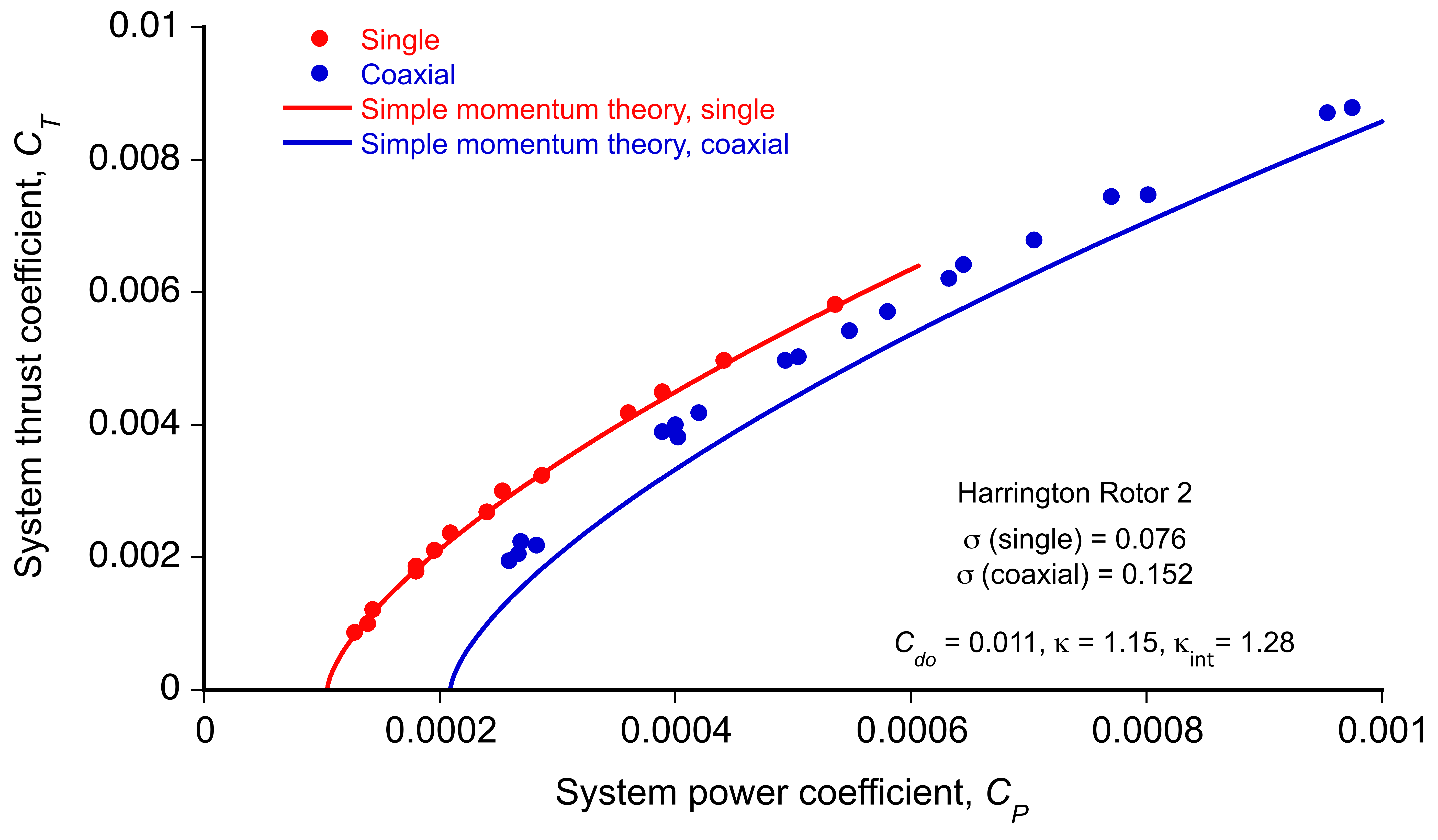
In each case, the two single rotors produce considerably better overall performance (better than 20%) than the coaxial rotor at all net thrust conditions, i.e., when carrying the same net weight. This result is an unambiguous confirmation of the rotor-on-rotor losses associated with a coaxial rotor system, regardless of how a figure of merit might be defined. Rotor 2 (with the higher solidity) is less efficient overall, both as a single and a coaxial.
However, remember that in practice, a single-rotor system will also incur additional losses from a tail rotor or other anti-torque system, typically about 10% of the net power. When this effect is considered, as a hovering system, the coaxial rotor can achieve a net aerodynamic efficiency comparable to that of the single-rotor and tail-rotor combination, but it is unlikely to be better. The coaxial rotor’s clear advantage is that it will always have a smaller diameter relative to a single rotor, generating the same thrust, but at the expense of 20% to 40% more power.
Notice that the momentum theory also always requires the a priori specification of , , and  , which must be assumed or derived empirically by baselining predictions against some known rotor performance. In this regard, the modified momentum theory only has a postdictive modeling capability.
Forward Flight Analysis
Under forward flight conditions, the rotor moves through the air with an edgewise velocity component parallel to the plane of the rotor disk. Under these conditions, the flow through the rotor loses its axisymmetry. Now, the flow field in which the rotor operates is considerably more complex than that of a fixed-wing, giving rise to several aerodynamic problems that ultimately limit the rotor’s performance.
Flow Environment
The overall aerodynamic complexity of the helicopter in forward flight can be appreciated from the schematic below. One issue is that blade tips on the advancing side of the rotor disk can enter supercritical and transonic flow regimes, leading to the formation of compressibility zones and, ultimately, strong shock waves. In addition, wave drag and the possibility of shock-induced flow separation must be considered, as the onset of either or both phenomena requires significantly more power to drive the rotor. The periodic formation of shock waves is also a source of obtrusive noise.
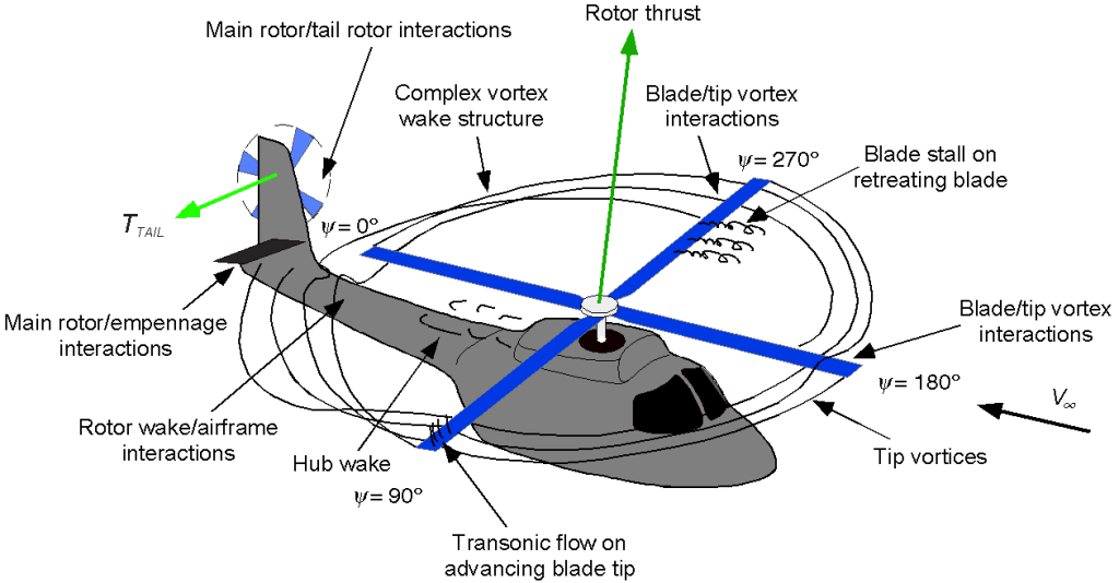
When compressibility effects manifest, the increased power demands on the rotor system will eventually limit forward flight speeds. Although compressibility effects on contemporary rotors can be somewhat alleviated by using swept-tip blades and thin “transonic” airfoils, the problems of increased power requirements and noise are only delayed to moderately higher forward flight speeds and are not eliminated.
Momentum Theory Analysis in Forward Flight
Despite the inherently more complex nature of rotor flow in forward flight, simple momentum theory can be extended under certain assumptions. Because helicopter rotors are required to produce both a lifting force (to overcome the helicopter’s weight) and a propulsive force (to propel the helicopter forward), the rotor disk must be tilted forward at an angle of attack relative to the oncoming flow. The following treatment of rotor performance in forward flight was first derived by Glauert, where the analysis is performed with respect to an axis aligned with the rotor disk, as shown in the figure below.
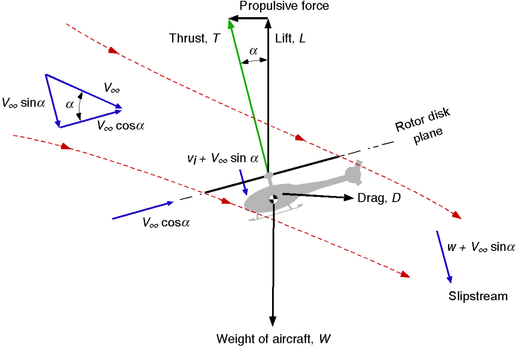
Mass Flow Rate
In this case, Glauert defines the mass flow rate, , through the actuator disk as
(105) 
where  is the resultant velocity at the disk as given by
(106) 
Thrust
The application of the conservation of momentum in a direction normal to the disk gives
(107) 
Power Required
By the application of conservation of energy, then
(108) 
(109) 
(110) 
giving  , the same relationship as the axial flight cases. Therefore,
(111) 
Notice that for hovering flight,  , so that Eq. 111 reduces to the result for hover (Eq. 7), i.e.,
(112) 
As forward flight speed increases such that  , then Eq. 111 reduces to
(113) 
which is called Glauert’s “high-speed” approximation.
The rotor thrust is given by
(114) 
which can be written as
(115) 
Recall from Eq. 112 that for hovering flight  , so the induced velocity in forward flight becomes
(116) 
The idea of a tip speed ratio or advance ratio,  , can now be introduced. By using the velocity parallel to the plane of the rotor, it is defined as
(117) 
In most cases, the value of  is sufficiently small so that
(118) 
Inflow
The inflow ratio is  so
so
(119) 
Also, Eq. 116 becomes
(120) 
But, it is also known from the hover case that  , therefore,
(121) 
Finally, the solution for the inflow ratio,  , is
, is
(122) 
This is a form of implicit equation in that the unknown value, , appears on both sides.
While analytic solutions to Eq. 122 can be found under certain assumptions, using a numerical method to solve for is preferable. The simplest approach is a fixed-point iteration. The algorithm consists of a loop that iteratively computes new estimates of until a termination criterion is met. To this end, Eq. 122 can be written as the iteration equation
(123) 
where  is the iteration number. The starting value for
  is usually the hover value (i.e.,
  ). The error estimator is
(124) 
and the convergence criteria is when  . Typically, between 10 and 15 iterations are required for convergence.
Results for the inflow ratio  computed are shown in the figure below for several different values of (both positive and negative) and over a range of values of
  typical of a helicopter, i.e.,
(125) 
or
(126) 
The induced part of the total inflow decreases with increasing advance ratio, but the total inflow increases and becomes dominated by the  term at higher advance ratios.
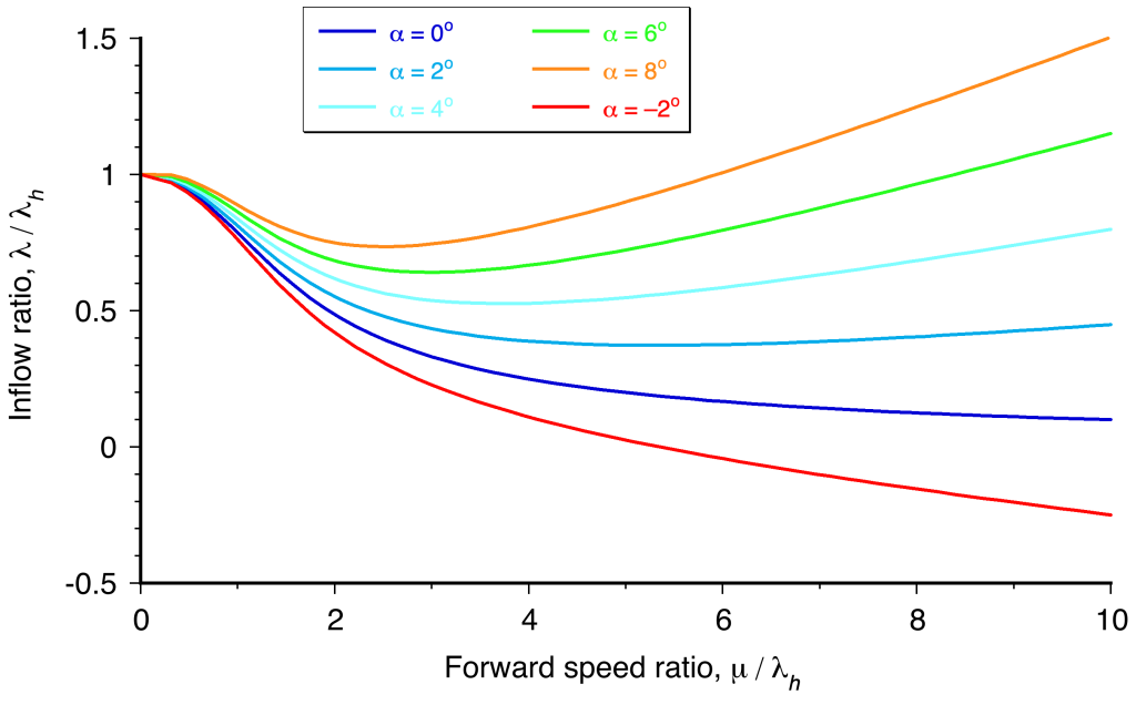
Power Requirements in Forward Flight
The rotor power in forward flight is given by
(127) 
The first term on the right-hand side of the above equation is the power required to propel the rotor forward and climb. The second term is the induced power. As for the axial flight case, the rotor power in forward flight can be referenced to the hovering result, and so
(128) 
Recall that
(129) 
Therefore,
(130) 
The first term on the right-hand side of the above equation is the extra power to meet propulsion and climb requirements, whereas the second is the induced power.
The inflow and power required for flight depend on the disk angle of attack, which must be slightly forward for propulsion to occur. This, in turn, requires knowledge of the helicopter’s drag, . Assuming straight-and-level flight, the disk angle of attack, , can be calculated from a simple force equilibrium, as shown in the figure below.
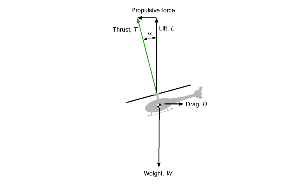
For vertical equilibrium  , and for horizontal equilibrium
  . Therefore, the disk angle of attack can be found from
(131) 
Therefore, the power equation in straight-and-level flight can be written as
(132) 
However, determining the drag on the helicopter requires knowledge of both the rotor drag and the airframe drag, the latter known as parasitic drag. The rotor drag must be estimated using blade-element theory.
Forward Flight Performance
For a helicopter in level forward flight, the total power required at the rotor, , can be expressed by
(133) 
where  is the induced power, is the profile power required to overcome viscous losses at the rotor, and
  is the parasitic power required to overcome the drag of the helicopter. Each contributing part can now be analyzed, and its effects combined.
Induced Power
The induced power of the rotor, , is given by
(134) 
or in coefficient form
(135) 
where is the now-familiar empirical correction for many non-ideal effects. The value of cannot necessarily be assumed independent of the advance ratio. Still, using a mean value between 1.15 and 1.25 is usually sufficiently accurate for preliminary predictions of power requirements.
Substituting the value of in forward flight gives
(136) 
Notice that if the forward velocity is sufficiently high, say  , then the induced velocity can be approximated by Glauert’s “high-speed” asymptotic result, i.e.,
(137) 
Profile Power
The profile power coefficient can be approximated as
(138) 
which is based on the blade-element theory, where the numerical value of  depends on the assumptions and approximations used in the blade-element integration.
In practice, a value of  is often used for helicopter performance predictions for
  . At higher advance ratios, experimental evidence suggests that profile power grows more quickly than given by Eq. 138 as a result of radial and reverse flow and compressibility effects on the rotor.
Parasitic Power
The parasitic power, , is a power loss from the drag on the airframe, rotor hub, etc. This drag source can be significant because helicopter airframes are much less aerodynamic than their fixed-wing counterparts, often with regions of large-scale flow separation.
The parasitic power contribution can be written as
(139) 
where  is some reference area and
  is the drag coefficient based on this reference area. In nondimensional form, this becomes
(140) 
where is the rotor disk area, and  (
( ) is known as the equivalent wetted area or equivalent flat-plate area. This area parameter accounts for the drag of the hub, fuselage, landing gear, and so on in aggregate.
The concept of the equivalent wetted area comes from noting that while the drag coefficient can be written in the conventional way as
(141) 
where is a reference area, the definition of may not be unique. Thus, an equivalent wetted area is used, which is defined as
(142) 
Such an approach avoids any confusion that could arise from defining different reference areas.
It is found that values of range from about 10 ft (0.93 m) on smaller helicopters to as much as 50 ft (4.65 m) on large utility helicopter designs.
Tail Rotor Power
The power required by the tail rotor typically varies between 3% and 5% of the main rotor power in routine flight and up to 20% at the extremes of the flight envelope. It is calculated similarly to the main rotor power, with the required thrust equal to the value necessary to balance the main rotor torque reaction on the fuselage. Using vertical tail surfaces to produce side force in forward flight can help reduce the power required by the tail rotor, albeit at the expense of increased parasitic and induced drag.
The interference between the main rotor, the tail rotor, and the vertical fin should be addressed even in an initial analysis. These effects may be accounted for by an increase in the induced power factor, , to take into account the generally higher nonuniform inflow at the tail rotor location. Although tail rotor power consumption is relatively low, interference effects may increase power requirements by up to 20%, depending on the tail rotor and fin configuration. Because the tail rotor consumes relatively little power, the power required for initial performance estimates can be expressed as a fraction of the total main rotor power, with a reasonable estimate of 5%.
Total Power
In light of the preceding, the total power coefficient for the helicopter in forward flight can be written in the form
(143) 
The tail rotor power must always be added to obtain a proper estimate of total helicopter power requirements. For larger values of , then  , so that Glauert’s formula allows Eq. 158 to be simplified to
(144) 
Comparison with In-Flight Measurements
The figure below presents representative results of the net power required for an exemplary helicopter in straight-and-level flight. A gross weight of 16,000 lb (7,256 kg) and an operating altitude of 5,200 ft (1,585 m) have been assumed. The rotor disk angle of attack was calculated at each airspeed to satisfy the horizontal force equilibrium, which, although not a complete trim calculation, provides reasonably acceptable results. The predicted components of the total rotor power are also shown, including that of the tail rotor. The helicopter’s equivalent flat-plate area, , is 23.0 ft (2.137 m). For both the main and tail rotors, it is assumed that  and
and  . The distance between the main and tail rotor shafts,
  , is 32.5 ft (9.9 m).
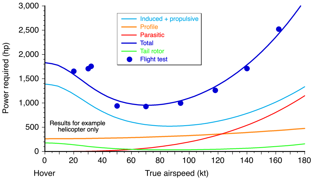
Notice that the induced and propulsive parts of the power initially decrease with increasing airspeed but increase again as the disk is progressively tilted forward to meet more significant propulsion requirements. It is insufficient to assume that induced losses are solely a result of lift generation; therefore, induced losses decrease rapidly with airspeed to a point, then increase again because of losses associated with propulsive forces.
The power required for forward flight increases quickly at higher airspeeds because the parasitic losses are proportional to  . The power growth rate is even higher when reverse flow and compressibility losses on the rotor are taken into account. However, the airframe drag significantly contributes to the total power required at high airspeeds. In design practice, much can be done to expand the flight envelope by striving for a more streamlined airframe.
Reverse Flow Region
In forward flight, a region of the rotor disk is on the retreating side called the “Reverse Flow Region.” In this region, the flow over the rotor blade section comes from tail to nose rather than nose to tail, as shown in the figure below. Because the flow in this region is “reversed” with the sharp trailing edge pointed into the airflow, the lift is negative, and the profile drag on the blade section will contribute somewhat more to the overall rotor torque and power required. The effects can usually be neglected at lower airspeeds.
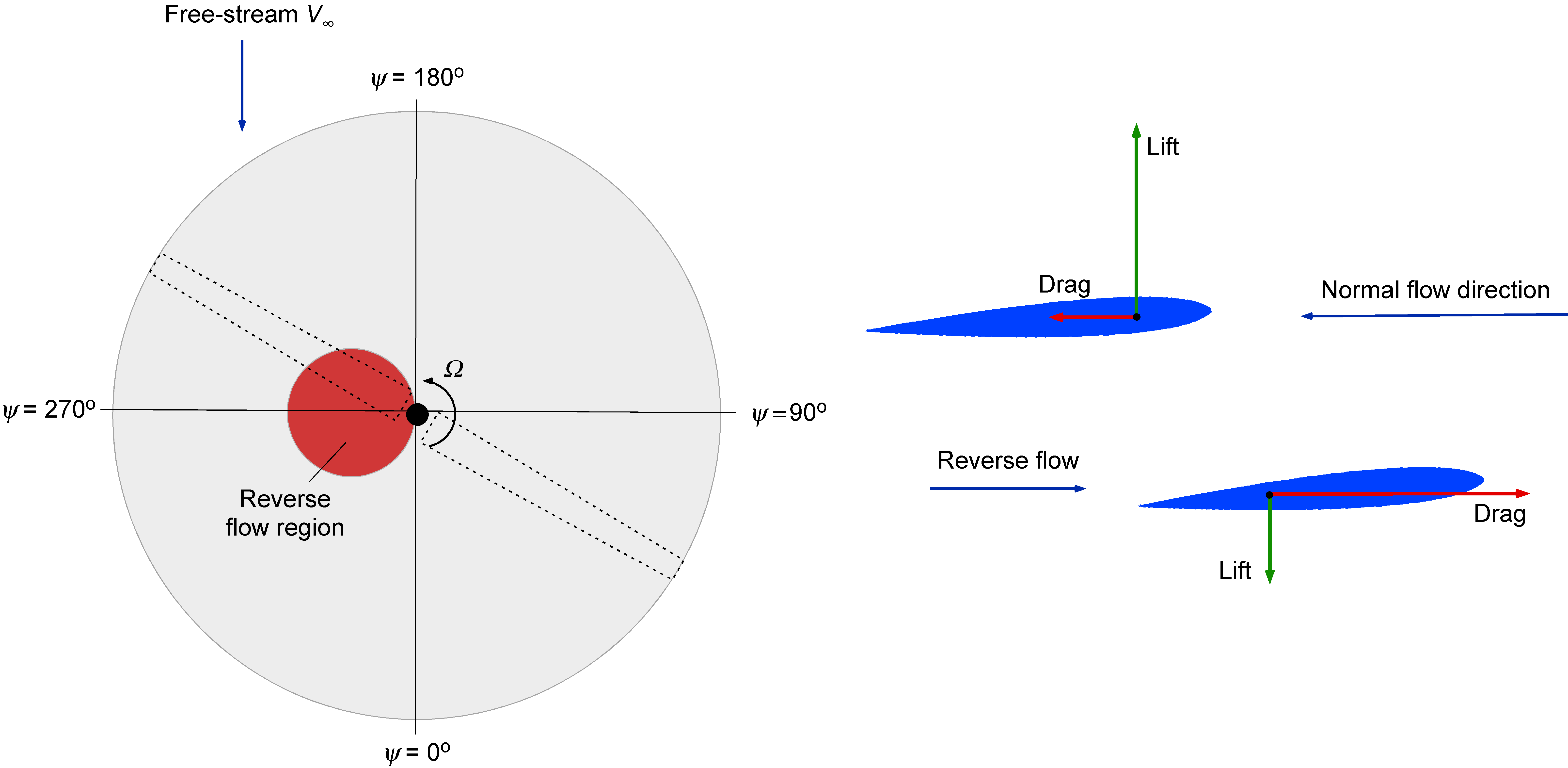
The geometry of this reverse flow region can be calculated using Eq. 2 with  , i.e.,
(145) 
This means that
(146) 
and for the boundary of the reverse flow region, then
(147) 
with  , which is the equation of a circle in polar coordinates with a center located at
  .
.
Effects of Weight
Representative results illustrating the effect of the helicopter’s weight on required power are presented below for the exemplar helicopter at mean sea level (MSL) conditions. Notice that higher flight weights require more power. In this case, the power available at MSL is 2,800 hp, and for a turboshaft engine, this stays relatively constant with airspeed.
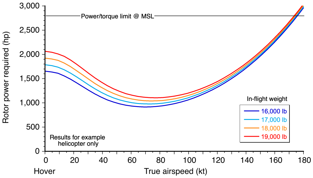
The airspeed at the intersection of the power required curve with the available power or torque curve gives the maximum flight speed. Most helicopters powered by turboshaft engines may be torque-limited, meaning the gearbox and transmission are the limiting factor rather than the engine’s shaft power. However, the maximum airspeed may also be determined by the onset of rotor stall and compressibility effects before it is reached.
Effects of Density Altitude
The effect of altitude on performance is a crucial operational consideration for any airplane. As shown in the figure below, increasing density altitude increases the power required in hover and at lower airspeeds. Lower air density results in a lower power requirement because of the reduction of parasitic drag at higher altitudes, i.e., because  .
.
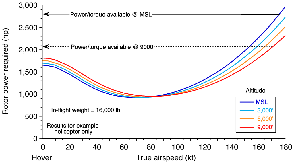
However, a higher density altitude will also affect the available engine power. At 9,000 ft, the power available is about 25% less than that available at sea-level conditions, resulting in a significant decrease in the excess power available at any airspeed relative to that at sea-level conditions. Again, remember that helicopters powered by turboshaft engines may be torque-limited, a limitation of the gearbox and transmission rather than the engine’s shaft power.
Climb Performance
The general power equation can be used to estimate the climb velocity, , that is possible at any given airspeed based on the excess power available, i.e.,
(148) 
It is realistic to assume that for low rates of climb or descent, the rotor-induced power, , the profile power, , and the airframe drag, , remain nominally constant, so
(149) 
Notice that  is simply the net power required to maintain level flight conditions at the same forward speed. If the available installed power is
  (which may vary with flight conditions), it will be observed that the power available for climbing varies with forward flight speed. The climb velocity can then be obtained from
(150) 
where  is the excess power available at that combination of airspeed and altitude.
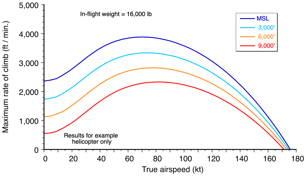
Calculations of the maximum rate of climb as a function of flight speed and density altitude are shown in the figure below for the exemplary helicopter. Notice that climb performance is substantially affected by density altitude. These curves will mimic the excess power available because the climb (or descent) velocity is determined simply by the excess (or decrease) in power required, , relative to steady-level flight conditions. Notice that the rate of climb improves significantly when transitioning from hover to forward flight. Pilots often refer to the tendency of a helicopter to climb when accelerating from hover as “translational lift.” However, the term is a misnomer because the helicopter climbs because of the excess power available, not extra rotor lift.
Check Your Understanding #7 – Power required in forward flight
A helicopter is operating in level forward flight at a true airspeed of 210 ft/s under the following conditions: shaft power supplied = 655 hp, = 6,000 lb,  = 0.00200 slugs/ft
 . The rotor parameters are = 19 ft, = 0.08,
  = 700 ft/s, , and = 0.01. Neglect the effects of reverse flow, stall, and compressibility. (i) How much power is required to overcome induced losses? (ii) How much power is required to overcome profile losses? (iii) What is the equivalent flat-plate area, ? (iv) If the installed power is 800 hp, estimate the maximum rate of climb possible at this airspeed.
Show solution/hide solution.
(i) The induced power of the rotor, , can be approximated by
![\[ P_i = \kappa T v_i \]](https://eaglepubs.erau.edu/app/uploads/quicklatex/quicklatex.com-e0ccb724163c33ffa361b17c9d86e2a4_l3.svg "Rendered by QuickLaTeX.com")
If the forward velocity is above  (
( in this case), then Glauert’s “high-speed” formula can approximate the induced velocity. Therefore, the induced power required does not need a solution to the inflow equation and can be determined from
![\[ P_i = \kappa T \left(\frac{T}{2 \varrho \, A \, V_{\infty}} \right) = \frac{\kappa W^2}{2 \varrho \, A \, V_{\infty}} \]](https://eaglepubs.erau.edu/app/uploads/quicklatex/quicklatex.com-5cfb69f56d6f7a2c62373983237a03f9_l3.svg "Rendered by QuickLaTeX.com")
Substituting the appropriate parameters gives the induced power at this operating condition as
![\[ P_i = \frac{ 1.15 \times (6,000)^2}{2 \times 0.002 \times \pi \times (19)^2 \times 210.0} \times \frac{1}{550} = 79.0 \mbox{hp} \]](https://eaglepubs.erau.edu/app/uploads/quicklatex/quicklatex.com-de4b0169da223b6b93503897b9de7dab_l3.svg "Rendered by QuickLaTeX.com")
(ii) The profile power coefficient can be estimated from
![\[ C_{P_{0}} = \frac{\sigma \, C_{d_{0}}}{8} ( 1 + K \mu^2) \]](https://eaglepubs.erau.edu/app/uploads/quicklatex/quicklatex.com-0a286f1693da0be98d07344e8d8ac3d9_l3.svg "Rendered by QuickLaTeX.com")
where can be assumed to be 4.7; different values may be assumed for . Therefore, at this operating condition, the profile power is

(iii) The total power in forward flight is the sum of induced, profile, and parasitic power, i.e.,
![\[ P = P_i + P_0 + P_p \]](https://eaglepubs.erau.edu/app/uploads/quicklatex/quicklatex.com-c58ee250da5c2948cd47b493826b1622_l3.svg "Rendered by QuickLaTeX.com")
Knowing the induced, parasitic, and total shaft power supplied means the parasitic power will be = 655 – 79.0 – 201.3 = 374.7 hp. The parasitic power coefficient can be written as
![\[ C_{p_{p}} = \frac{1}{2} \left( \frac{f}{A} \right) \mu^3 \]](https://eaglepubs.erau.edu/app/uploads/quicklatex/quicklatex.com-a97743024df848fdd1654b106b1659fb_l3.svg "Rendered by QuickLaTeX.com")
where is the equivalent parasitic drag area. In dimensional units, the parasitic power is
![\[ P_p = \frac{1}{2} \varrho \, f \, V_{\infty}^3 = 0.5 \times 0.002 \, f \, 210^3 = 374.7 \times 550 \]](https://eaglepubs.erau.edu/app/uploads/quicklatex/quicklatex.com-487e5d725b54b0600bbf2a4a78aac617_l3.svg "Rendered by QuickLaTeX.com")
Solving for gives
![\[ f = \frac{2 \times 374.7 \times 550}{0.002 \times 210^3} = 22.25~\mbox{ft${^{2}}$} \]](https://eaglepubs.erau.edu/app/uploads/quicklatex/quicklatex.com-2f2316f2a18da4f1efb5123ae3b2e09b_l3.svg "Rendered by QuickLaTeX.com")
(iv) The maximum rate-of-climb, , is determined by the excess power available over and above that required from a straight-and-level flight at the same airspeed. In this case
![\[ V_c = \frac{\Delta P}{W} = \frac{ (800 - 655 ) \times 550}{6,000} = 13.26~\mbox{ft/s} \]](https://eaglepubs.erau.edu/app/uploads/quicklatex/quicklatex.com-83974a6022fd03b3279f851da0e3d0b0_l3.svg "Rendered by QuickLaTeX.com")
Conventionally, in aviation, this result would be expressed in terms of feet per minute, giving  60 = 798 ft/min.
Fuel Flows
For many aircraft performance problems, such as range and endurance calculations, knowledge of the engine’s fuel burn(s) is required. From the power required curves for the helicopter, the fuel consumption can be estimated for any given engine type, such as a piston or turboshaft engine. Engine performance characteristics are usually expressed in terms of brake-specific fuel consumption or BSFC (in units of lb hp hr or kg kWhr) versus shaft power (in units of hp or bhp or kW). These curves depend on atmospheric conditions, so a set of curves is required for different altitudes and operating temperatures. Fuel flow curves must be derived as a function of indicated airspeed and gross weight.
For a normally aspirated (non-supercharged) piston (reciprocating) engine, the power curves vary almost linearly with the density ratio, . One common approximation is
(151) 
where  is the power available at altitude and
  is the power available at mean sea level conditions. The value of the density ratio can be determined from the ISA model, which depends on pressure altitude and outside air temperature.
For a turboshaft engine, a good approximation is
(152) 
where  is the pressure ratio at that altitude and
  is the corresponding absolute temperature ratio, which can be found from the ISA model.
Because helicopters will operate with their engines running at close to their rated power for much of the flight, a first-level approximation is to assume that the brake-specific fuel consumption (BSFC) remains independent of power output. In this regard, the fuel flow rate  is given by
(153) 
where is the total power required for the helicopter at altitude. Generally, fuel flow curves versus airspeed (at a given density altitude) are fairly flat. Therefore, for most helicopters, the fuel flow curves will mimic the shapes of the power-required curves. In this regard, a representative fuel flow curve for a helicopter is shown in the figure below. Notice that the best flight endurance occurs at the airspeed with the lowest fuel burn rate. The best range will occur at the airspeed corresponding to the lowest fuel burn per unit distance, as obtained at the tangent point, as shown. Notice this is because
(154) 

Range & Endurance
The fuel flow curves provide the information to determine range/payload and endurance/payload charts. These charts provide critical information on aircraft range and endurance, particularly when balancing payload and fuel, and will be used by pilots for flight planning. Helicopters have a relatively low functional load capability compared to airplanes, so the payload trade-off with fuel is usually severe. Specific mission profiles for any aircraft must be defined when calculating flight endurance and range, although most missions will involve a flight from point A to point B. Engine characteristics must be considered to determine maximum endurance and range, specifically the brake-specific fuel consumption (BSFC).
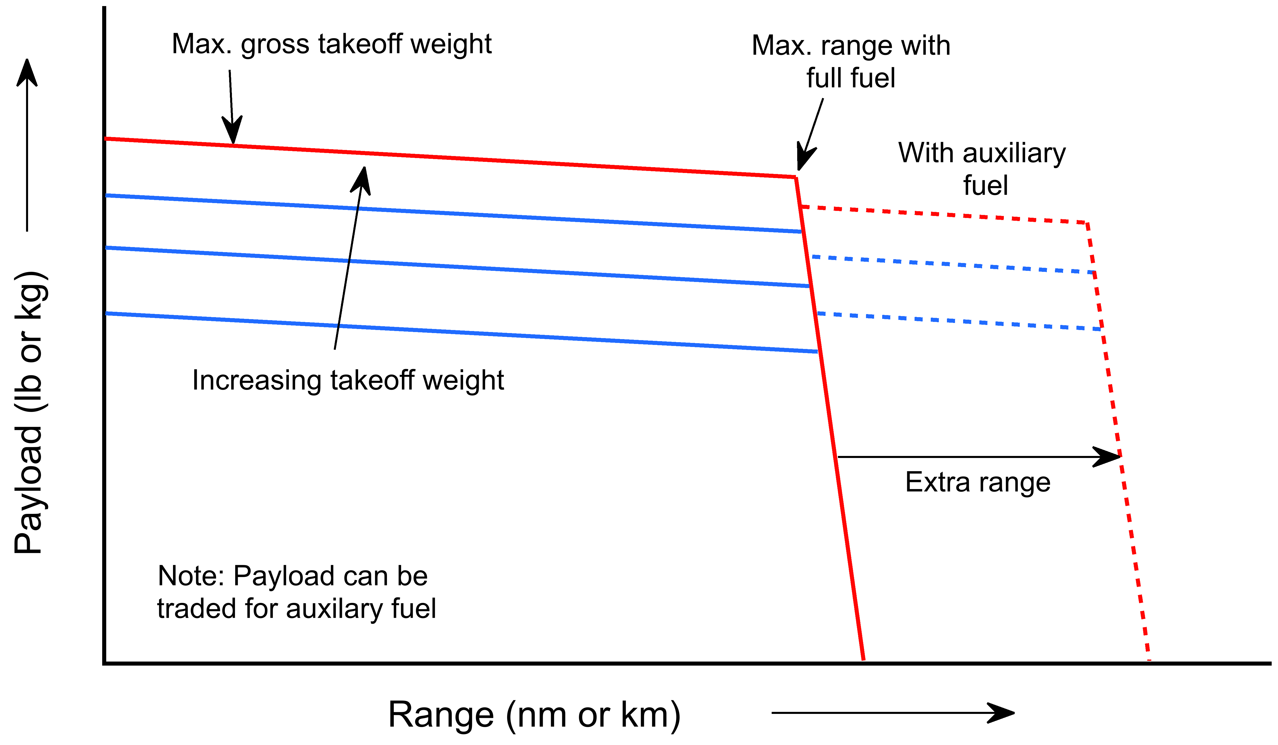
The fuel burn rate,  , with respect to distance, , will be
(155) 
where BSFC is the specific fuel consumption of the engine(s). The required power, , varies with gross weight and density altitude, and, as already shown, the BSFC itself depends on both. Because the weight decreases as fuel is burned, Eq. 155 must be integrated numerically to find the range. Fuel burned during takeoff, climb, and descent is factored into the calculation, along with a mandated fuel reserve in minutes of flying time. Because the fuel weight on a helicopter is normally a small fraction of the total gross weight, the fuel burn rate can be evaluated fairly accurately at the point in the cruise where the aircraft weight is equal to the initial gross weight (gross takeoff weight  ) is less half the initial fuel weight, where is the initial fuel weight. In this case, the range, , of the helicopter is given by
(156) ![\begin{equation*} R = W_F \left[ \frac{V_{\infty}}{P \times \rm {BSFC}} \right]_{W=W'} \end{equation*}](https://eaglepubs.erau.edu/app/uploads/quicklatex/quicklatex.com-06b6d0197e85e9db0479646ab83fedb4_l3.svg "Rendered by QuickLaTeX.com")
less an allowance for the other contingency factors described previously.
By a similar process, the estimated endurance,  , will be given by
(157) ![\begin{equation*} E = W_F \left[ \frac{1}{P \times {\rm BSFC} } \right]_{W=W'} \end{equation*}](https://eaglepubs.erau.edu/app/uploads/quicklatex/quicklatex.com-50aea07149fa789685a411a4e53cc0b5_l3.svg "Rendered by QuickLaTeX.com")
Generally, estimating endurance by dividing the usable fuel onboard by the average fuel flow rate is a sufficiently accurate method.
Coaxial Rotor in Forward Flight
As previously explained, counter-rotating coaxial rotors incur an additional induced power when the lower rotor operates in the wake of the upper rotor. This unavoidable loss occurs irrespective of whether the two rotors operate at the same thrust or torque. In this case, the total power equation in forward flight can be written as
(158) 
where is the induced power factor that accounts for rotor-on-rotor interference. The inflow for two closely spaced coaxial rotors, which share the same inflow, can be calculated as the total thrust of the system, in a manner similar to the performance of a single rotor using the inflow equation. In this case, using = 1.28 would be appropriate.
Measurements of coaxial rotor performance in forward flight are rare. However, the Harrington 1 coaxial rotor, as described previously, was tested in a NACA wind tunnel by Dingledein. The figure below compares the momentum theory with measured rotor performance levels. Notice that the theory generally slightly overpredicts the power requirements for the single rotor and underpredicts the power required for the coaxial rotor system. Such performance trends have also been shown using other predictive methods.
Any differences between the measured and predicted power values with the coaxial rotor are at least partly due to uncertainties in how the rotor was trimmed (collective and cyclic pitch). These uncertainties are compounded by some uncertainty in determining the equivalent parasitic drag area, which determines the rotor shaft angle in the wind tunnel and, thus, the equivalent parasitic component of power required to overcome drag. To this end, notable uncertainties are apparent in the measurements.
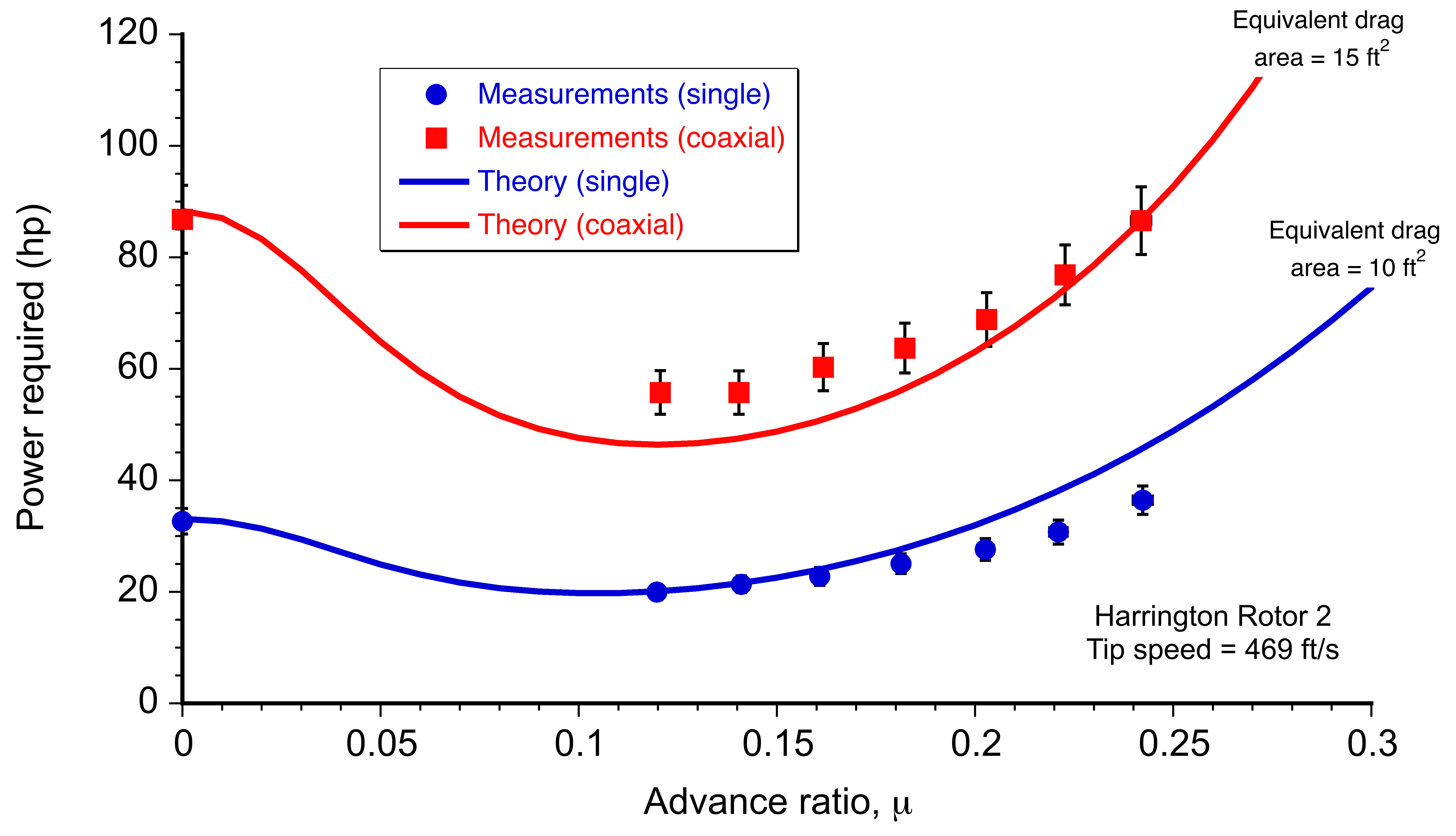
While the agreement between theory and measurements for a coaxial rotor is not perfect, momentum theory can provide reasonable predictions of coaxial rotor performance, at least for preliminary design in both hover and forward flight. It should be noted, however, that uncertainties will always exist in the predicted performance of any rotorcraft utilizing a coaxial rotor system, particularly when actual flight test data are unavailable for validation. As flight test results are obtained, it will be possible to retroactively refine predictions of rotor loads and aircraft performance (including range, endurance, etc.) by incorporating empirical refinements into various aerodynamic theories (e.g., providing more accurate estimates of profile drag coefficients and equivalent parasitic drag area). In particular, accurately determining the aircraft’s parasitic drag will be critical for estimating performance.
Blade Element Theory
The blade element theory (sometimes denoted BET in many texts) provides estimates of how aerodynamic forces vary radially along a rotor blade’s span. As shown in the schematic below, the blade is idealized as a collection of infinitesimally small, independent elements, each acting as a quasi-two-dimensional airfoil that produces local values of lift and drag. The BET can be used for both hovering and forward-flight analysis and serves as the basis for many comprehensive analyses in rotorcraft design.
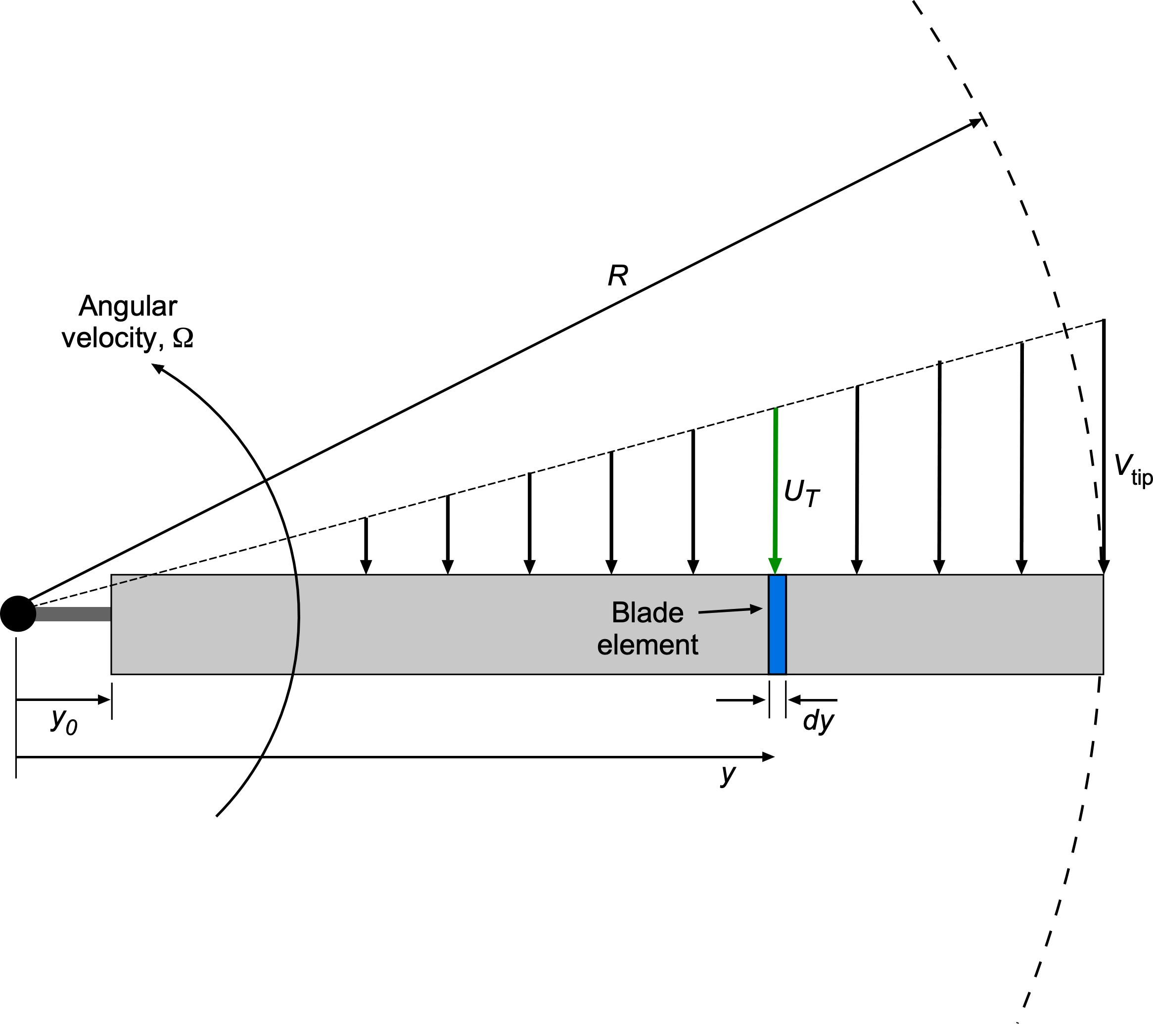
At each blade element, the relative flow velocities determine the elemental components of the local lift and drag, which can be resolved into corresponding elemental contributions to thrust and torque (or power), as shown in the blade element diagram below. The in-plane velocity, i.e., the velocity in the plane of rotation of the rotor, is denoted by  and the out-of-plane velocity by
  . These components are vectorially combined to determine the resultant flow velocity and the blade section’s angle of attack. Notice that besides the angle of attack, the lift and drag will also be functions of the local Mach number and Reynolds number.
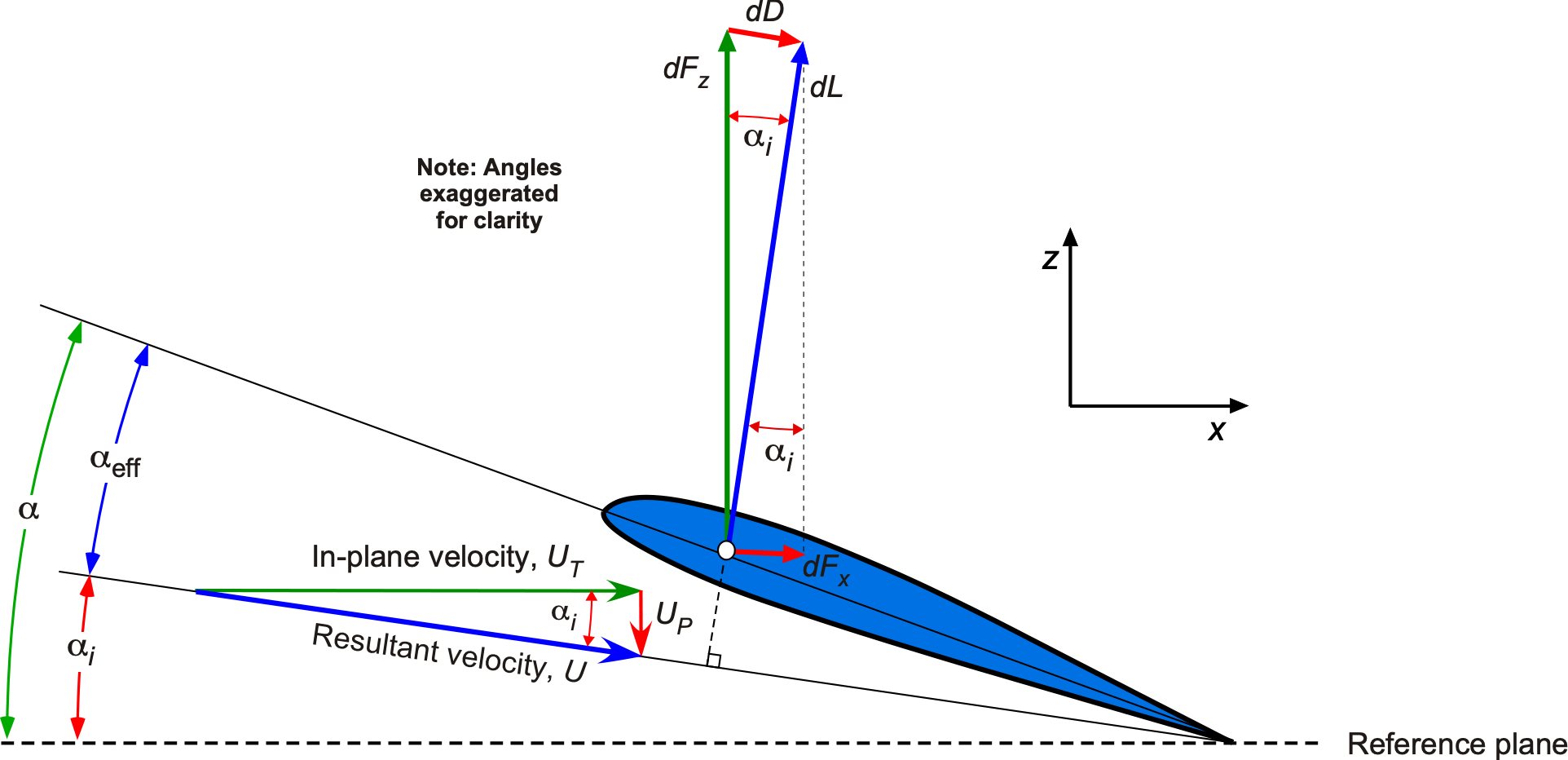
Once these sectional loads are determined, the total thrust, torque, and power can be obtained by integrating their contributions along the blade span and averaging in time over a rotor revolution. This approach allows the BET to serve as a practical framework for incorporating the effects of blade twist, planform shape, and airfoil selection in determining rotor performance metrics. The method can also be used to help achieve a desired level of rotor performance during the design process, e.g., determining the blade shape in terms of planform, twist, and airfoil section.
Formulation
In the blade-element method, the primary source of three-dimensional effects arises in the non-uniformity of the induced inflow from the rotor wake, which modifies the local angle of attack at each blade element; if the induced velocity distribution over the rotor disk is known or can be reasonably approximated, then the aerodynamic loads at each spanwise location follow straightforwardly. Furthermore, three-dimensional effects near the blade tip, commonly referred to as tip loss, are accounted for using established types of correction factors, as will be discussed in detail later.
Consider a blade element located at a radial station  . For hovering flight, the in-plane velocity, , at the element is
(159) 
and the out-of-plane velocity is
(160) 
where is the climb velocity and is the induced velocity. In general, will depend on both the radial position along the blade, , as well as the azimuth angle , i.e.,  . The resultant velocity is
(161) 
The inflow angle  is
is
(162) 
which reduces the effective angle of attack at the element to
(163) 
where is the pitch angle at that blade section. Notice that the blade may be twisted, so  . The incremental lift and drag per unit span are
(164) 
where  and
and  are the local lift and drag coefficients, respectively, with
  being the local chord. These forces are resolved into components normal and tangential to the rotor disk (considered as the reference plane) according to
(165) 
The elemental contributions to thrust, torque, and power are then, respectively,
(166) 
where is the number of blades.
Simplifications
To simplify the analysis for hover or axial flight, it is acceptable to note that  except near the root, so
  . Also, is small, so
  and
and  , and that
  , allowing the
  term to be neglected. Under these approximations, then
(167) 
Introducing a nondimensional span defined by and local solidity  , the elemental thrust coefficient becomes
(168) 
and the incremental torque coefficient is
(169) 
Because  , then the latter equation can be written as
(170) 
The total thrust and power coefficients then follow by spanwise integration.
For rectangular blades with constant chord, a common assumption in the development of analytic results for instructional purposes, then
(171) 
It will be noticed that because  , then the numerical values of the coefficients and are identical. Evaluating these latter expressions requires knowledge of the inflow distribution
  and the sectional aerodynamic coefficients
  and
and  .
.
Thrust Approximations
With the assumption of a linear aerodynamic behavior at each blade station, the sectional lift coefficient is described by
(172) 
where  is the lift-curve-slope and
  is the local blade pitch angle. Notice that in axial flight, then can be written as
(173) 
From Eq. 168, the elemental thrust coefficient is
(174) 
so substituting  gives
gives
(175) 
Integrating over the span gives
(176) 
because  . Some special canonical cases can now be evaluated.
Untwisted Blades
With constant pitch then  and with the assumption of uniform inflow
  = constant, then
(177) ![\begin{equation*} C_T = \frac{1}{2}\, \sigma \, C_{l_\alpha} \left[ \theta_0\int_0^1 r^2\,dr - \lambda\int_0^1 r\,dr \right] = \frac{1}{2}\sigma \, C_{l_\alpha} \left( \theta_0 \, \frac{1}{3} - \lambda \, \frac{1}{2} \right) \end{equation*}](https://eaglepubs.erau.edu/app/uploads/quicklatex/quicklatex.com-f9e1b9e0a815ad735fddca9c1371f313_l3.svg "Rendered by QuickLaTeX.com")
or
(178) 
Linearly Twisted Blades
For a linearly distributed blade twist the  , so that
(179) ![\begin{equation*} C_T = \frac{1}{2}\, \sigma \,C_{l_\alpha} \left[ \int_0^1 (\theta_0 r^2 + \theta_{\rm tw} r^3)\,dr - \lambda\int_0^1 r\,dr \right] = \frac{1}{2}\, \sigma \,C_{l_\alpha} \left( \theta_0\, \frac{1}{3} + \theta_{\rm tw}\,\frac{1}{4} - \lambda\,\frac{1}{2} \right) \end{equation*}](https://eaglepubs.erau.edu/app/uploads/quicklatex/quicklatex.com-6fda6035f08d8315ea6ddf33465727c1_l3.svg "Rendered by QuickLaTeX.com")
again assuming uniform inflow to obtain this result. Therefore,
(180) 
Notice that equating the thrust to that of an untwisted blade then
(181) 
If the blade pitch is measured relative to the 3/4-radius, then
(182) 
which gives the root pitch as
(183) 
Substituting into the thrust expression gives
(184) 
so that the thrust is the same as for an untwisted blade with the pitch set to  , i.e., the value at the 3/4-radius location.
Ideal Twist
From momentum theory, with a uniform pressure jump over the disk, the incremental thrust is
(185) 
where is the disk area. In terms of thrust coefficient, then
(186) 
From blade element theory, neglecting profile drag, the incremental thrust coefficient is
(187) 
Equating the momentum theory and blade-element results gives
(188) 
giving
(189) 
With , then
(190) 
Imposing the tip condition  gives
gives
(191) 
Therefore, the required twist varies hyperbolically over the blade span, which is the classic ideal blade twist that minimizes the induced power.
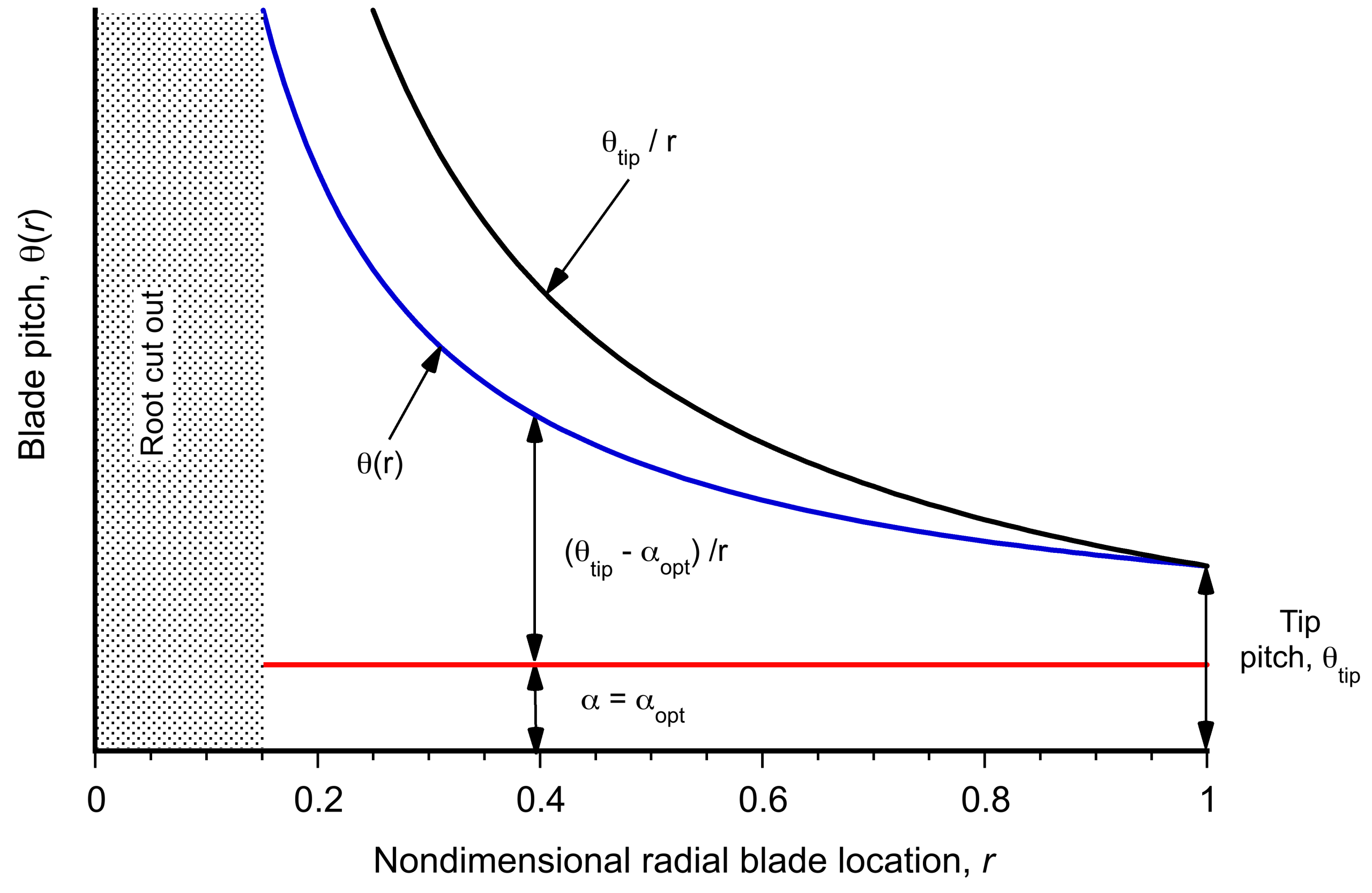
Thrust Versus Blade Pitch
In hover, the uniform inflow ratio from momentum theory is
(192) 
which can be combined with the thrust expressions to relate the required collective pitch to a prescribed thrust coefficient in hover. For small angles, the local inflow angle is  , so the local angle of attack is
(193) 
The sectional lift coefficient is  , and the differential thrust coefficient in hover can be written as
(194) 
so that the thrust coefficient becomes
(195) 
For a blade with uniform pitch  , the thrust coefficient in hover is
(196) 
Solving explicitly for the required collective pitch for a given gives
(197) 
Notice that the relationship between  and is nonlinear in that the slope of the
  curve becomes increasingly steep with increasing .
For a blade with linear twist referenced to the root, then
(198) 
the thrust coefficient becomes
(199) 
It is convenient to define an equivalent pitch
(200) 
so that the thrust relation has the same form
(201) 
and the equivalent pitch needed for a given is
(202) 
If the twist  is specified, then the required root pitch is
(203) 
It is often convenient to specify the pitch at the  radius as together with a linear twist , so that
(204) 
Substitution into the thrust integral gives
(205) 
so for a uniform inflow and constant solidity, the total hover thrust depends only on the pitch at  and not explicitly on the twist. The required pitch at for a given is
(206) 
These nonlinear relationships are shown in the figure below. At low thrust levels, the square-root term dominates and thrust increases only slowly with pitch, whereas at higher thrust levels the linear term dominates. Differentiating the pitch with respect to gives
(207) 
so the sensitivity of pitch to changes in thrust is always positive. The inverse slope, which gives the change in thrust coefficient with respect to changes in pitch, is
(208) 
or, equivalently,
(209) 
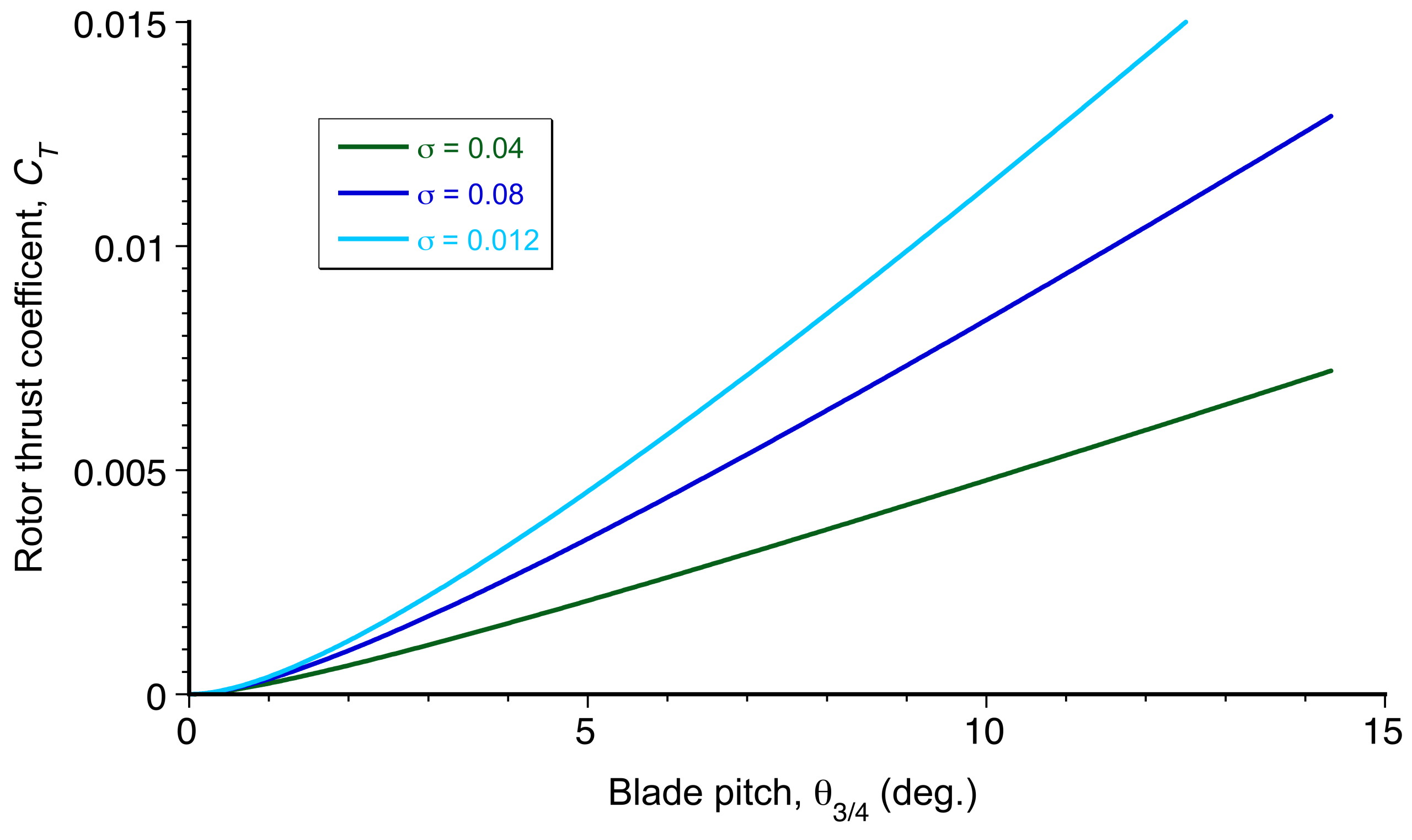
As  , the term
  becomes large, so
  tends to zero and the versus curve is very shallow near the origin. As the value of increases, the square root term becomes less important, and the slope becomes
(210) 
Power Approximations
From the definition of the torque coefficient, then
(211) 
where the first term represents the induced power and the second is the profile power. With uniform inflow and constant drag coefficient , then
(212) 
so that
(213) 
Recall that in the simple momentum theory, then  and so
(214) 
Therefore, the blade element theory recovers the same result from momentum theory under the assumption of uniform inflow, with the now familiar additional profile-power term  being included.
Induced Power Factor
In the simple momentum theory, the induced power factor must be assumed or evaluated from measurements. However, the blade element theory provides a direct method for calculating the induced power factor if the loading distribution on the blades can be determined. For reference, in hover, the momentum theory gives disk area integrals for thrust and induced power as
(215) 
where the area element is  . Defining the uniform inflow reference for the same thrust as
(216) 
then the induced power factor is defined by  , giving
(217) 
For illustration, it is convenient to assume a power-law inflow given by  with
with  . Then
(218) 
and
(219) 
Hence
(220) 
Using  then
then
(221) 
Therefore, the induced power factor can be expressed as
(222) 
This result gives  for uniform inflow and
  for
for  . Although this is an idealized result, it highlights the significance of the blade-element theory for calculating quantities that are not accessible within the framework of simple momentum theory.
Tip-Loss Effects
The concept of tip-loss has already been discussed, acknowledging that, due to the formation of the trailing tip vortex, the tip region of the blade generates significantly less lift than a two-dimensional blade section. A simple tip-loss model assumes the lifting radius is reduced by a factor  , giving an effective span
  . Repeating the thrust integration with the limits
  to gives
(223) 
and for ideal twist  , then
(224) 
A more consistent and physical interpretation is that tip loss increases the required induced velocity by  , giving
(225) 
Including nonuniformity and tip-loss through a factor gives the induced-power approximation
(226) 
In this form, the tip loss appears explicitly in the induced power factor. Writing the net induced part as  , the tip loss model implies that
(227) 
For tip loss alone, the induced power is increased by the factor , so the additional tip-loss increment is
(228) 
Therefore, the net induced-power factor is taken as the sum
(229) 
and the total hover power coefficient becomes
(230) ![\begin{equation*} C_P=\kappa_{\rm net}\,\lambda_0\,C_T+ \frac{1}{8}\sigma \, C_{d_0} =\Bigg[\kappa+\left(\frac{1}{B}-1\right)\Bigg]\lambda_0\,C_T + \frac{1}{8}\, \sigma \, C_{d_0} \end{equation*}](https://eaglepubs.erau.edu/app/uploads/quicklatex/quicklatex.com-e19b937cc02b8bd0668d2ad5d5381251_l3.svg "Rendered by QuickLaTeX.com")
Profile Losses
Momentum theory accounts only for induced losses, and the profile (section) losses of the blades must be added. These losses arise from the drag on the airfoil sections as they sweep through the air, and exist even if the rotor produces zero thrust. Unlike induced power, which depends on the global flow the rotor itself creates, profile power depends on local sectional aerodynamics, i.e., the blade chord, the airfoil shape, the Reynolds and Mach numbers, and the distribution of drag coefficient along the span.
Rectangular Blades
In hover/axial flight, with  , the elemental profile power is
(231) 
Integrating from to and setting  and
and  , then
(232) 
With  and
and  , then
(233) 
With a root cutout ( ), then integrating from
  to gives
(234) 
Equivalently,
(235) 
where  . This result reduces to
(236) 
for  , which is the classic power equation used in many forms of rotor analysis.
Minimizing Profile Losses
Consider a blade with ideal twist in which the blade pitch is given by
(237) 
So the local angle of attack becomes
(238) 
and the sectional lift coefficient is
(239) 
Because this expression states that the local lift coefficient increases hyperbolically toward the root, rotor performance will ultimately be limited by the onset of stall at some inboard radius  where
where  .
.
Therefore, minimize the total profile losses on the rotor, the goal is to modulate the spanwise loading so that  remains close to the value that gives the best aerodynamic efficiency, i.e., the blade sections operate at the optimum angle of attack and lift coefficient for the best lift-to-drag ratio, i.e.,
(240) 
The differential thrust on the rotor in hover is
(241) 
For the minimum induced losses, the spanwise loading is
(242) 
so if  , then
(243) 
which requires
(244) 
Equivalently, the chord must satisfy
(245) 
which increases the chord hyperbolically toward the root to ensure , as shown in the figure below
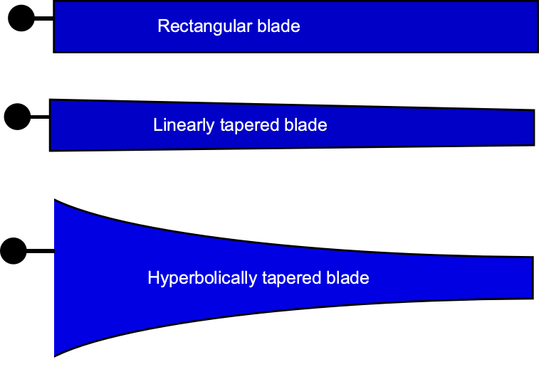
Using a general parabolic drag polar, i.e.,  , the local profile power is
(246) 
With  and
and  , this becomes
(247) 
so the profile power is generated primarily through the  weighting when the blade has hyperbolic taper. In the special case of constant chord
  and constant
  , one recovers the classic result that
(248) 
or
(249) 
At fixed thrust and radius, minimizing profile losses while preserving the ideal induced loading is achieved by holding
(250) 
and choosing
(251) 
With  , the elemental profile power coefficient becomes
(252) 
Using the tip solidity  gives
gives
(253) 
Integrating from  to
to  then gives
(254) 
so
(255) 
This result shows that, with a blade having , the profile power coefficient is increased by a factor of  compared to the constant-chord case, even though tapering the blade in this ideal manner would ordinarily be expected to reduce the profile power.
The fault in this analysis lies with the definition of the comparable reference blade area and the assumption previously used that  equals the chord of the rectangular blade. To make more sense, the results need to be compared based on the same equivalent areas where
  , which brings up the concept of equivalent rotor solidity. The local solidity is defined as
(256) 
and the equivalent solidity (thrust-weighted) is defined as
(257) 
The principle here is that sections of the blade further away from the rotational axis experience higher aerodynamic loads, so their aerodynamic effects are stronger than those of the blade section at the blade root.
For a rectangular blade with constant chord ,  so
so
(258) 
For a hyperbolic variation in chord or  , then
(259) 
Equal values of equivalent solidity requires that  and so
  . With and
  , the profile power coefficient is
(260) 
For the rectangular blade, then
(261) 
so at equal values of equivalent solidity, then
(262) 
Optimum Hovering Rotor
An optimum hovering rotor has a hyperbolic taper to minimize profile losses and a hyperbolic twist to minimize induced losses. The uniform inflow reference comes from the simple momentum theory, i.e.,
(263)
The total power coefficient is the sum of the induced and profile parts, i.e.,
(264) 
so the figure of merit is
(265) 
For an optimum hovering rotor, the ideal twist produces the minimum induced losses, i.e.,  . For a rectangular, untwisted blade, the spanwise loading is non-ideal and the induced power factor is greater than unity, i.e.,
  . As previously used, a convenient parametric representation of the non-uniform inflow is
  , giving
(266) 
so  corresponds to ideal loading
  and gives
  . Using the thrust-weighted equivalent solidity, the hyperbolically tapered blade satisfies
(267) 
Because  and
and  , then
  .
.
It should be appreciated that although the optimum hovering rotor provides minimum induced power in vertical flight through its hyperbolic twist, hyperbolic taper, and uniform inflow distribution, these same features make it unsuitable for forward flight, where the rotor moves edgewise through the air.
The hyperbolic blade twist becomes inconsistent with the asymmetric inflow distribution in forward flight, resulting in excessively high angles of attack on the retreating side and small or even negative angles of attack on the advancing side. The aerodynamic performance, therefore, deteriorates, and less twist must be used to balance forward-flight and hovering performance.
A hyperbolic taper also places too much area and pitch near the blade root, where the in-plane velocity is small, leading to premature stall and large torsional and vibratory loads. Moreover, the higher solidity required for the hover optimum greatly increases profile power and advancing-side drag at finite advance ratios.
Because the induced velocity field in forward flight contains substantial azimuthal and radial variations that a hover-optimized geometry cannot accommodate, the classical optimum hovering rotor becomes aerodynamically unsuitable and must be replaced by a compromise design suited to both hover and forward flight.
Blade Element Analysis in Forward Flight
Forward flight introduces several physical features that fundamentally alter the blade-element formulation compared with hover. Most importantly, the velocity field seen by each blade element varies with azimuth. As the blade advances and then retreats relative to the free-stream, the local airspeed, inflow angle, and aerodynamic angle of attack vary periodically. A second key feature is that the induced inflow becomes azimuthally nonuniform because the rotor wake is skewed and convected downstream. Both effects must be incorporated to obtain a consistent forward-flight blade element theory.
Let be the blade azimuth angle measured in the rotor plane, and let  be the nondimensional radial coordinate. The free-stream velocity is
  , the rotor angular velocity is , and the rotor radius is . The nondimensional advance ratio is
(268) 
The in-plane velocity seen by the blade element consists of the rotational term  and the projection of the free-stream velocity onto the rotor disk, i.e.,
(269) 
The out-of-plane velocity contains the induced inflow, the kinematic effect of blade flapping, and the vertical projection of the free-stream motion. Denoting the induced velocity by  and the blade flapping displacement by
  , i.e.,
(270) 
where
(271) 
is the nondimensional induced inflow. The inflow angle is  , and the instantaneous aerodynamic angle of attack becomes
(272) 
where  is the blade pitch distribution. This expression explicitly shows how forward flight produces a periodic variation in angle of attack around the azimuth.
The sectional lift and drag are evaluated from the angle of attack using the same aerodynamic relations introduced in the hover analysis. The resulting sectional forces resolved normal and tangential to the rotor disk are
(273) 
Let be the number of blades. The thrust and torque are obtained by integrating these forces over radius, as for the hover case, but now they must also be averaged over the azimuth, i.e., for the thrust, then
(274) 
and for the torque, then
(275) 
Recall that the power is given by  .
.
Thrust & Power
In forward flight, the rotor experiences nonuniform inflow and blade flapping. The azimuthal variation of induced inflow is represented using a first-harmonic Fourier series attributed to Glauert, i.e.,
(276) 
As shown previously, the first harmonic blade flapping can be expressed as
(277) 
The coefficients ,  ,
,  and the flapping coefficients
  ,
,  ,
,  are determined from the flapping hinge moment condition, periodicity, and the chosen inflow model for
  .
.
The evaluation of the rotor thrust requires the azimuthal average of the in-plane velocity squared. Using  gives
gives
(278) 
The average of the mixed product  is
is
(279) 
Substituting these averages gives the thrust coefficient as
(280) ![\begin{equation*} C_T = \frac{1}{2} \int_0^1 \sigma(r)\,C_{l_\alpha} \Big[ \theta(r)\left(r^2+\frac{1}{2}\,\mu^2\right) - r\,\lambda_0 - \frac{1}{2}\,\mu\,r\,\lambda_{1s} \Big] r\,dr \end{equation*}](https://eaglepubs.erau.edu/app/uploads/quicklatex/quicklatex.com-a3709f6d680dc23b40be245b10f2252d_l3.svg "Rendered by QuickLaTeX.com")
where  is the local rotor solidity. The elemental in-plane aerodynamic force is
(281) 
and the torque becomes
(282)
The induced portion of the power follows from the component of  proportional to the induced inflow. In blade-element form, it is the thrust-weighted mean inflow, i.e.,
(283) 
with
(284) 
The corresponding profile part of the power is
(285) 
so that
(286) 
Rectangular, Untwisted Blades
The solutions to the foregoing integrals are generally complicated and must often be computed numerically. However, analytic solutions can be obtained in some special cases. In the case of constant chord, constant solidity , and uniform pitch , the needed integrals can be shown to be
(287) 
Substitution gives
(288) ![\begin{equation*} C_T = \frac{\sigma\,C_{l_\alpha}}{2} \left[ \theta_0\left(\frac{1}{3}+\frac{\mu^2}{4}\right) - \frac{\lambda_0}{2} - \frac{\mu\,\lambda_{1s}}{4} \right] \end{equation*}](https://eaglepubs.erau.edu/app/uploads/quicklatex/quicklatex.com-d66f0781eedf4ce7764995c5755bfabf_l3.svg "Rendered by QuickLaTeX.com")
The induced and profile power coefficients are given by
(289)
and
(290) 
so
(291)
For small angles and a vertical shaft, Glauert’s first-harmonic inflow model gives
(292) 
Using  gives the closed form
(293) 
and hence
(294) 
The induced and profile power become
(295) 
so that
(296) 
As  , the uniform-inflow momentum relation gives
(297)
and the induced power reduces to the hover value
(298) 
and
(299) 
This first-harmonic representation of induced inflow provides a compact and tractable description of forward-flight aerodynamics, but it must be recognized as an approximation. The actual induced velocity field is highly nonuniform, with substantial variations across both radius and azimuth caused by the skewed and contracting wake. As the wake is swept downstream, the induced velocity seen by a blade element depends not only on its current azimuthal position but also on the history of vorticity shed into the wake. This history effect produces higher-order harmonic content in  and introduces spatial gradients that a single sine-cosine pair cannot represent.
Because of this behavior, the forward-flight inflow problem cannot be solved exactly using only closed-form momentum or blade-element methods. A fully self-consistent solution requires computing the wake geometry, the distribution of vorticity along it, and the resulting induced velocity at every blade element. Modern approaches, therefore, rely on numerical free-wake models, prescribed-wake geometries, or higher-order inflow states that augment the simple three-parameter model used here. These methods better reproduce the nonuniform character of the induced velocity in forward flight and provide more accurate predictions of thrust, power, and control loads.
The present development should therefore be regarded as the lowest-order analytical model that captures the essential physics of forward-flight inflow. It establishes the structure of the problem, identifies the dominant harmonics, and provides the foundation for more advanced rotor-wake models.
Blade Element Momentum Theory (BEMT)
Blade element momentum theory (BEMT) combines the local blade-element formulation with the previously developed one-dimensional momentum relations. The BEMT is an axial-flow theory for hover and vertical climb; it is analogous to the methods used in propeller theory. In this case, however, the momentum theory balance is applied to an elemental annulus of the rotor disk rather than to the disk as a whole, as shown in the figure below. The essential idea is to require that the incremental rotor thrust generated on each annulus of the rotor disk from momentum considerations equals the thrust produced by the blade elements that occupy that annulus. The outcome is profound in that a solution is now obtained to solve for the inflow distribution, thereby abandoning the requirement that the inflow in the blade element theory be known or assumed.
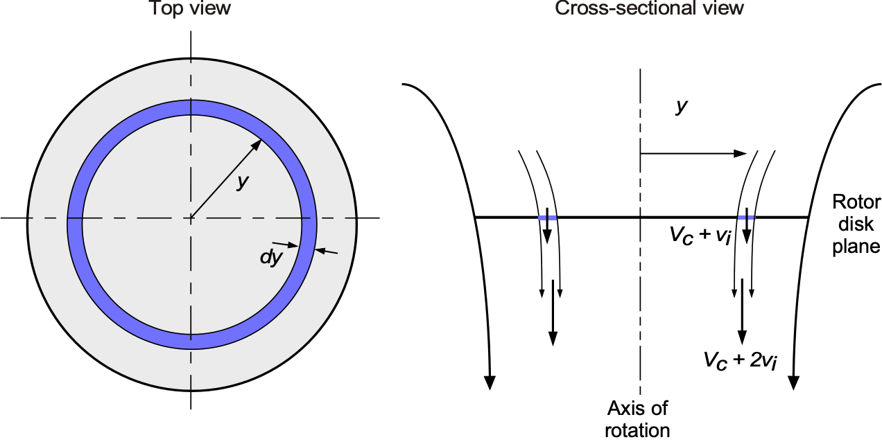
Consider an annulus of the rotor disk at radius with width  . The annular area is
  , so the mass flow rate through the annulus is
(300) 
where is the climb velocity and is the induced velocity at the disk. The incremental thrust on the annulus is then
(301) 
and in nondimensional form, the incremental thrust coefficient is
(302) 
From the blade element perspective, the incremental thrust coefficient on the same annulus can be written as
(303) 
where is the thrust-weighted solidity, is the local pitch angle,  is the sectional lift-curve slope, and the local angle of attack is
  with
with  .
.
Equating the thrust from Eqs. 302 and 303 gives
(304) 
which can be rearranged as
(305) 
This leads to a quadratic equation in terms of the inflow, i.e.,
(306) 
Solving Eq. 306 for gives
(307) 
In hover,  , so the BEMT inflow equation simplifies to
(308) ![\begin{equation*} \lambda(r) = \frac{\sigma C_{l_{\alpha}}}{16}\left[\sqrt{1 + \frac{32}{\sigma C_{l_{\alpha}}}\,\theta(r)\,r} - 1\right] \end{equation*}](https://eaglepubs.erau.edu/app/uploads/quicklatex/quicklatex.com-4c60e54b38a6c5d699ccb0df21d756d4_l3.svg "Rendered by QuickLaTeX.com")
Given the radial distributions of pitch, solidity, and airfoil lift-curve slope, Eq. 308 specifies the induced inflow as a function of radius. Substituting into the momentum expressions then gives the global thrust and induced power, i.e.,
(309) 
For an untwisted rectangular blade with constant , Eq. 308 predicts a nonuniform inflow that is larger toward the tip, which is associated with an induced power factor  . Recall that the ideal twist law produces uniform inflow and minimum induced power. If the product
  is constant, i.e.
(310) 
then Eq. 308 gives a constant inflow solution, i.e.,
(311) ![\begin{equation*} \lambda(r) = \frac{\sigma C_{l_{\alpha}}}{16}\left[\sqrt{1 + \frac{32\theta_{\rm tip}}{\sigma C_{l_{\alpha}}}} - 1\right] = \sqrt{\frac{C_T}{2}} \end{equation*}](https://eaglepubs.erau.edu/app/uploads/quicklatex/quicklatex.com-8eb7b94dcc18b7feae7f32bf1b3e1916_l3.svg "Rendered by QuickLaTeX.com")
As discussed in the blade element framework, this analytical result is frequently used as a design reference for an optimal hovering rotor, subject to the usual practical constraints on stall and inboard profile drag growth.
Numerical Solution to the BEMT
For general blade designs, the BEMT equations must be solved numerically. The blade is divided into  radial elements of span
  , as shown in the figure below, and the inflow is evaluated at the mid-span radius,
  , of each element, i.e.,
(312) ![\begin{equation*} \lambda(r_n) = \frac{\sigma C_{l_{\alpha}}}{16}\left[\sqrt{1 + \frac{32}{\sigma C_{l_{\alpha}}}\,\theta(r_n)\,r_n} - 1\right], \qquad n = 1,\dots,N \end{equation*}](https://eaglepubs.erau.edu/app/uploads/quicklatex/quicklatex.com-677d9e268302e880cdc76650e3ebcf36_l3.svg "Rendered by QuickLaTeX.com")
Within this BEMT framework, arbitrary radial variations in twist, chord, and section properties can be accommodated. Comment blade shapes include linear twist and taper; a linear twist distribution may be written as  , and a linear variation of local solidity (taper) as
  . In the BEMT, the blade shapes can be arbitrary and are not restricted to any canonical form.
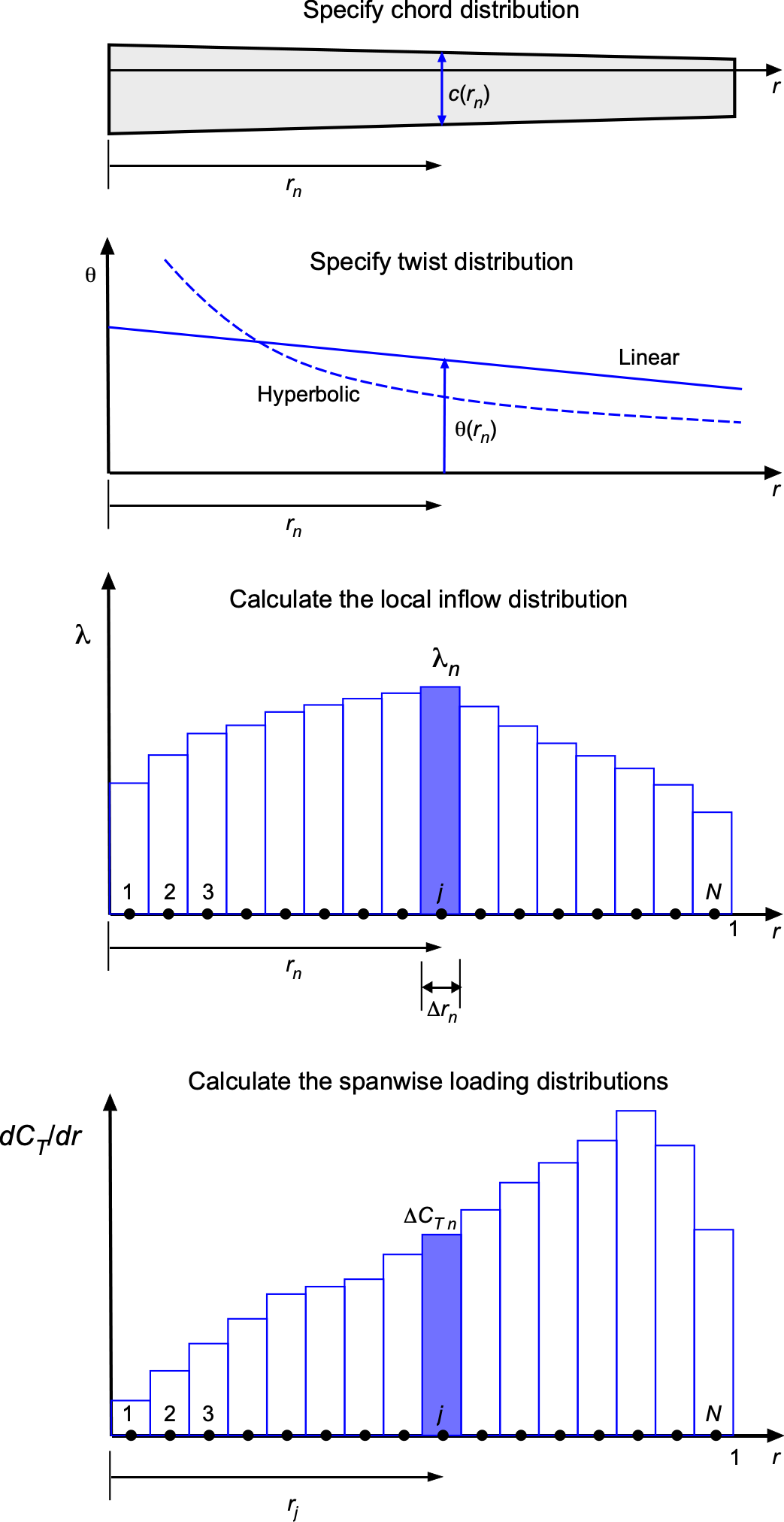
For tapered blades, the results should be compared at the same thrust-weighted solidity, i.e.,
(313) 
which should be held constant when comparing the effects of twist and taper on performance.
The incremental thrust coefficient is
(314) 
and the total thrust coefficient is obtained by numerical integration, for example, with the rectangle rule, then
(315) 
The induced power coefficient follows from
(316) 
The power is obtained as before from the airfoil drag coefficient ; if is treated as constant, then
(317) 
When using the BEMT, comparisons between different rotors with blades of different twist and planform should be made at the same thrust coefficient (or disk loading). For a blade with linear twist and uniform inflow, one convenient analytic relation is
(318) 
which can be solved for to get
(319) 
These expressions provide a useful starting guess for the collective pitch when iterating toward a target thrust coefficient  in a numerical BEMT method.
Checking the BEMT
The BEMT is a relatively simple algebraic solution, and the numerical results can be readily compared with the exact analytical solutions provided by the theory. A classic test case is a rotor with uniform chord and hyperbolic twist, which should recover the uniform-inflow case. Representative results are shown in the figure below for  and . Uniform inflow is also consistent with a linear distribution of thrust and torque (or power). Notice that for the uniform-chord case, the lift coefficient is hyperbolic across the span, increasing rapidly toward the root.
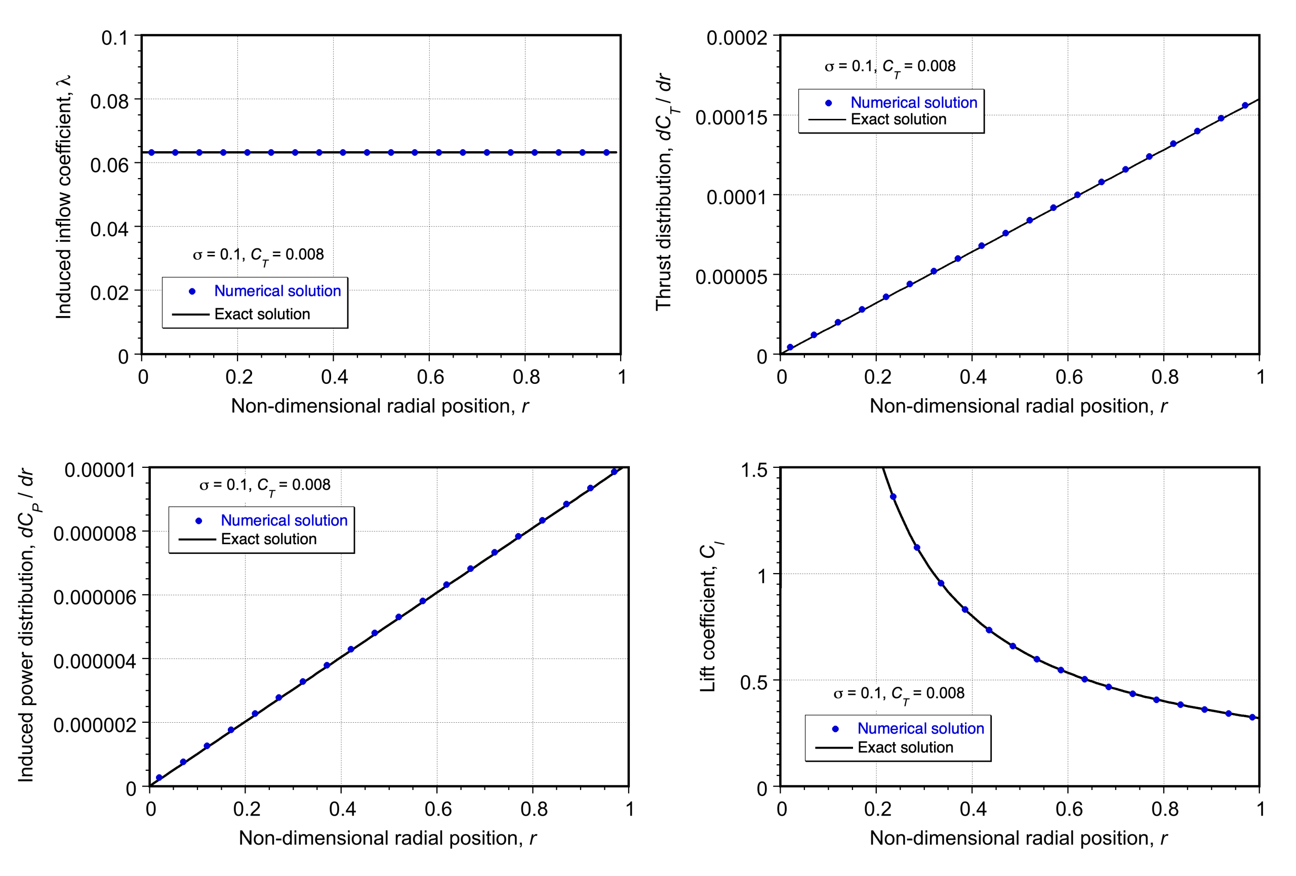
Finite Blade Number
The preceding development assumes an infinite number of blades. For a finite , the lift and induced velocity are reduced near the tip. Prandtl’s tip-loss function introduces this effect through a correction factor  in the annular momentum term, i.e.,
(320) 
where  is the local inflow angle. The momentum expression becomes
(321) 
and equating this with the blade element thrust gives
(322) 
or
(323) 
The corresponding inflow solution for the hover case is
(324) ![\begin{equation*} \lambda(r) = \frac{\sigma C_{l_{\alpha}}}{16F}\left[\sqrt{1 + \frac{32F}{\sigma C_{l_{\alpha}}}\,\theta r} - 1\right] \end{equation*}](https://eaglepubs.erau.edu/app/uploads/quicklatex/quicklatex.com-65f560145d2e15667b7ebc436d88208a_l3.svg "Rendered by QuickLaTeX.com")
Because depends on , this equation is solved iteratively, usually converging in just a few passes; usually, five is sufficient. The tip-loss correction increases the inflow near the blade tips, rolls off the tip loading, and increases the induced power; representative results are shown in the figure below. Increasing the number of blades reduces the tip loss, and in the limit of an infinite number of blades, the actuator disk results are obtained. However, the practical gains in rotor efficiency in using more than 4 or 5 blades are small.
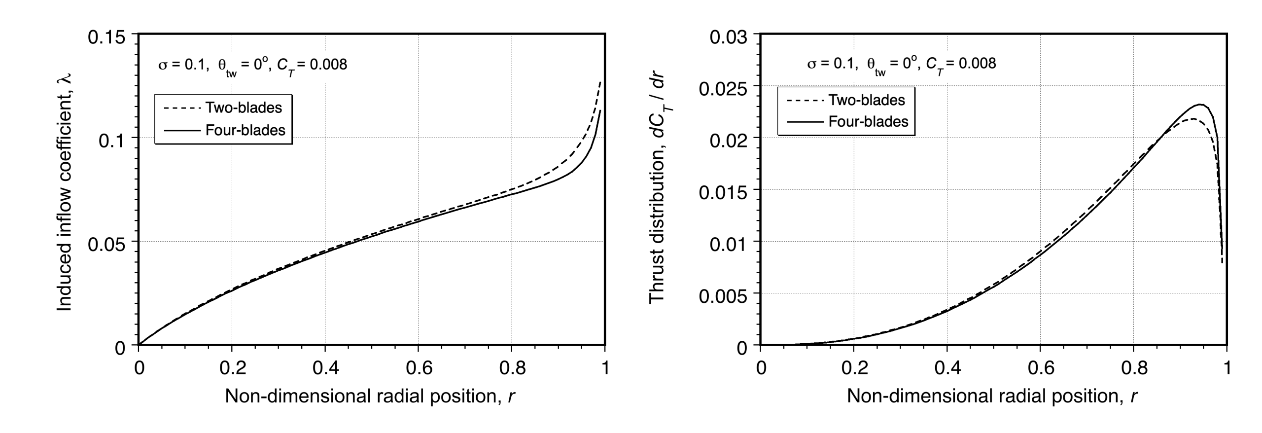
Effects of Twist & Taper
A moderate nose-down geometric blade twist tends to make the inflow more uniform, offload the outer part of the blade, reduce induced power, and shift the loading inboard toward the ideal triangular distribution (see the figure below). The inflow varies greatly from root to tip because the local blade element angle of attack increases toward the inner parts of the blade. Introducing some nose-down twist counteracts this tendency by reducing the pitch at the tip relative to the root, thereby flattening the spanwise lift distribution. Linear twist rates of 5 to 15 degrees work best, giving a more even inflow distribution, lower induced losses, and a lift distribution closer to the minimum-induced-loss ideal. The use of higher twist rates is detrimental.
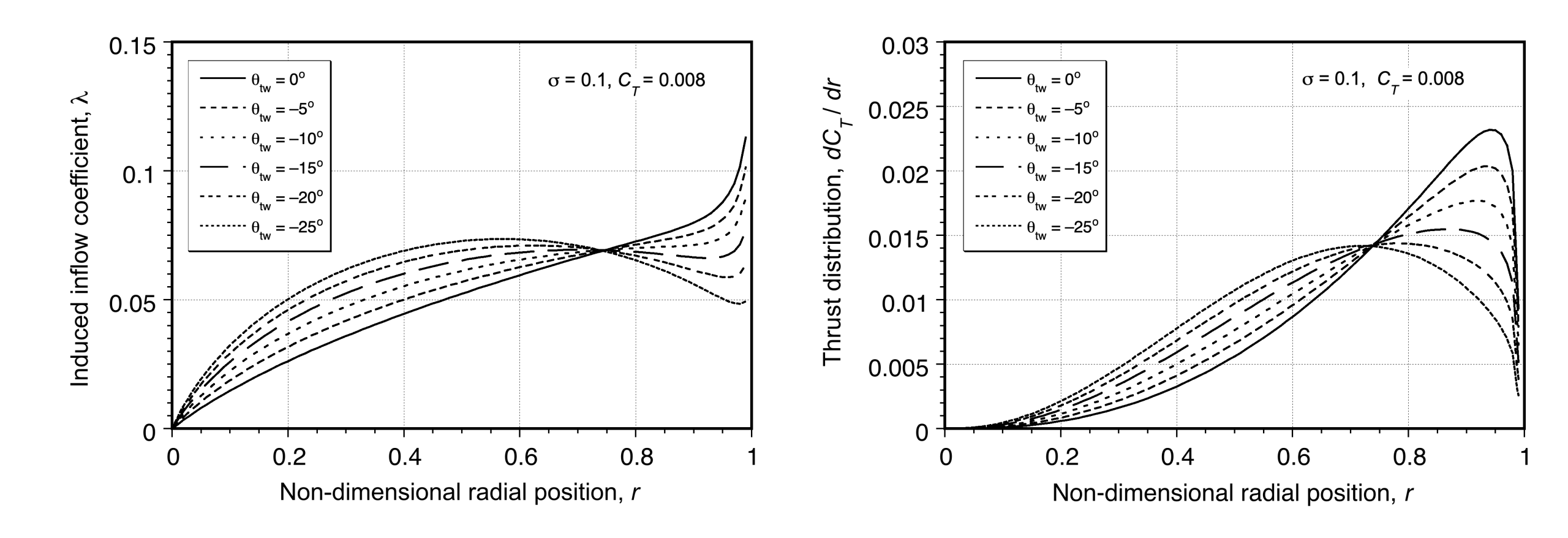
The reduction in induced power can be quantified by the induced power factor, often written as  . BEMT calculations show that depends not only on the rotor geometry but also on its operating thrust coefficient, as shown in the figure below. For a given twist, operating at higher values of generally improves the loading shape and reduces induced losses, whereas low-thrust operation tends to increase because of poorer inflow uniformity.
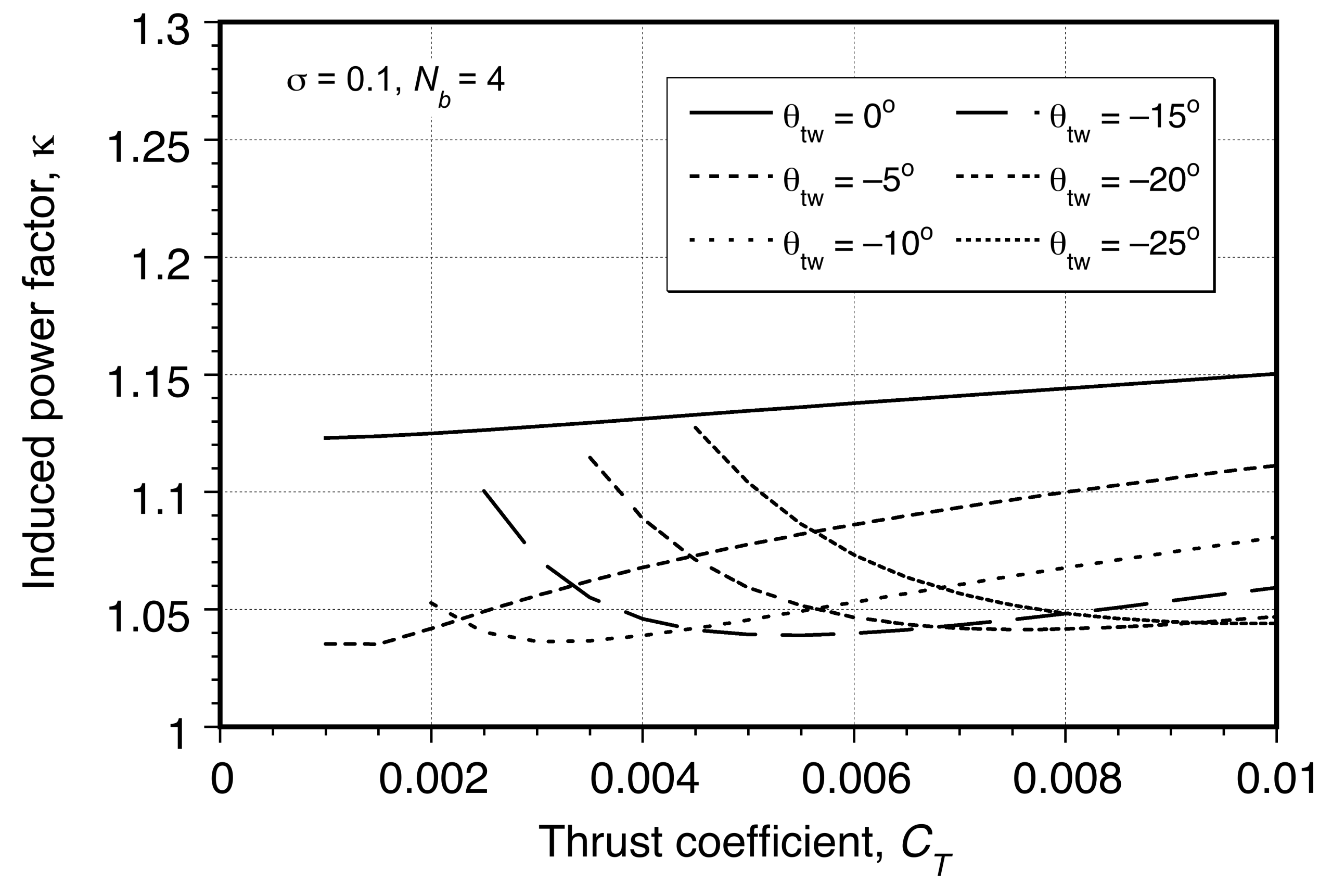
Tapering the blade along its span modifies the chord distribution in a way that complements twist. By reducing the chord near the tip, taper lowers the local Reynolds number only slightly but reduces the sectional lift coefficient required to produce the desired thrust, as shown in the figure below. This decreases the profile drag contribution in the outer region of the blade, where the local velocity is highest. At the same time, the larger chord retained inboard helps keep the sectional lift coefficients moderate and maintains favorable lift-to-drag ratios at the inner radii. Because stall typically initiates when the inboard region is required to carry excessive load, taper helps delay the onset of stall by redistributing the sectional lift coefficients more evenly.
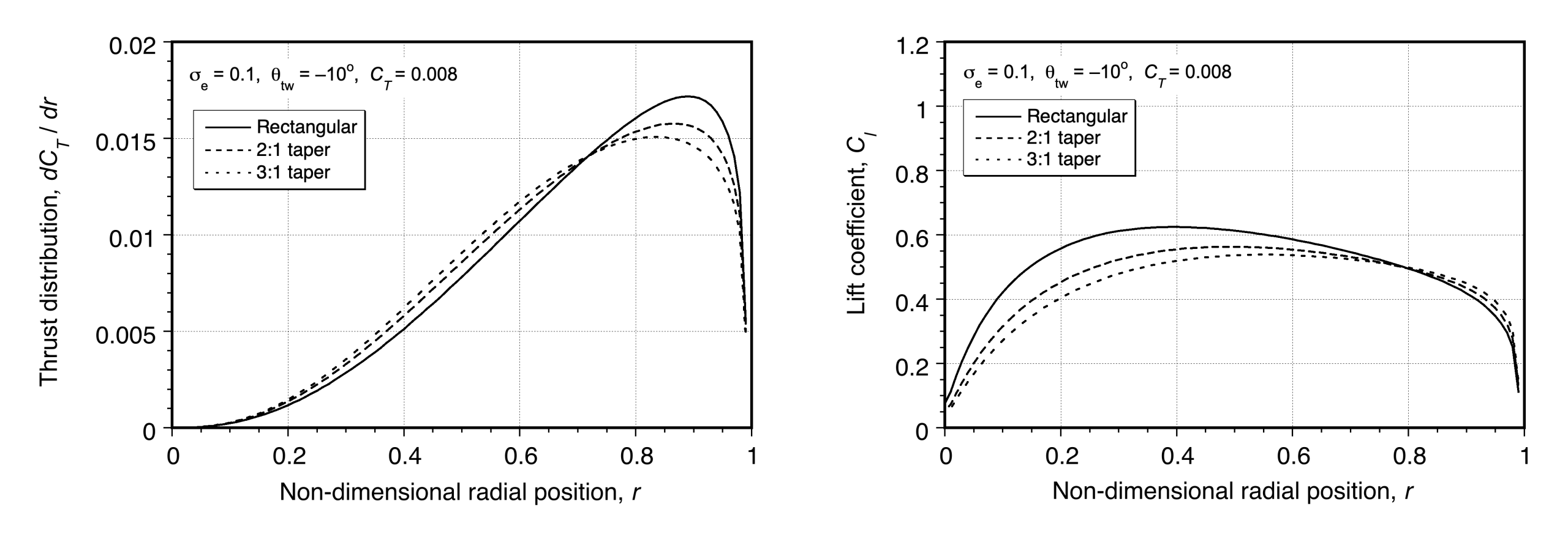
In combination, twist and taper allow the designer to decouple the two principal components of rotor power. Twist primarily affects induced power by shaping the lift distribution and the resulting inflow field. Taper primarily affects profile power by controlling the chord and the associated section drag. BEMT provides a practical, computationally efficient approach to examine these design trades, quantify the induced and profile contributions, and identify combinations of twist and taper that maximize the figure of merit for a specified thrust coefficient.
Controlling the Helicopter
One of the greatest mysteries to most people about helicopters is how they are controlled during flight. In the case of an airplane, control is much more intuitive because it is obtained by using easily identifiable aerodynamic surfaces, such as ailerons, elevators, and rudder, which are deflected to generate the appropriate forces and moments on the airplane during its flight. In a helicopter, control is achieved by using the forces and moments generated by the rotor, which are produced by tilting the rotor disk. The question now is how to do this.
Main Rotor
First, it can be shown that the dynamic natural frequency of a rotor blade in its flapping motion (up and down) about the flapping hinge is equal to the rotational frequency, . While this result is strictly valid for a blade with a hinge at the rotational axis, it is sufficiently accurate for any practical rotor. It does not alter the physics of the discussion that follows.
The critical issue is understanding that if any first-order dynamic system is excited by a forcing function at its natural frequency, it will respond at that frequency, but with a 90 phase lag between the forcing and the response. For example, in the case of a rotor blade, if its lift (the forcing) is increased, then the blade response (the flapping angle) does not change instantaneously but will increase over time and only reach its maximum flapping displacement 90 later. This 90 lag between changes in blade pitch (lift) and the flapping response (displacement) is the key to understanding how to control the helicopter.
A mechanism is required to adjust the blade pitch angles, thereby altering the blades’ lift. Most often, this is done using a swashplate, as shown in the photograph below. A swashplate consists of two plates: the upper one rotates with the rotor, and the lower one is fixed and connected to the pilot’s controls. The upper swashplate is connected to the blades using pitch links, so the movement of the swashplate (up and down and tilting) then translates into displacements of the pitch links, producing changes in the blade pitch angles. A set of bearings between the two disks allows the upper disk to rotate with the rotor, while the lower disk remains stationary. Both disks can be slid up and down the shaft in response to collective pitch inputs, and the swashplate can also be tilted to an arbitrary orientation in response to cyclic pitch inputs, both of which originate from the pilot’s controls.
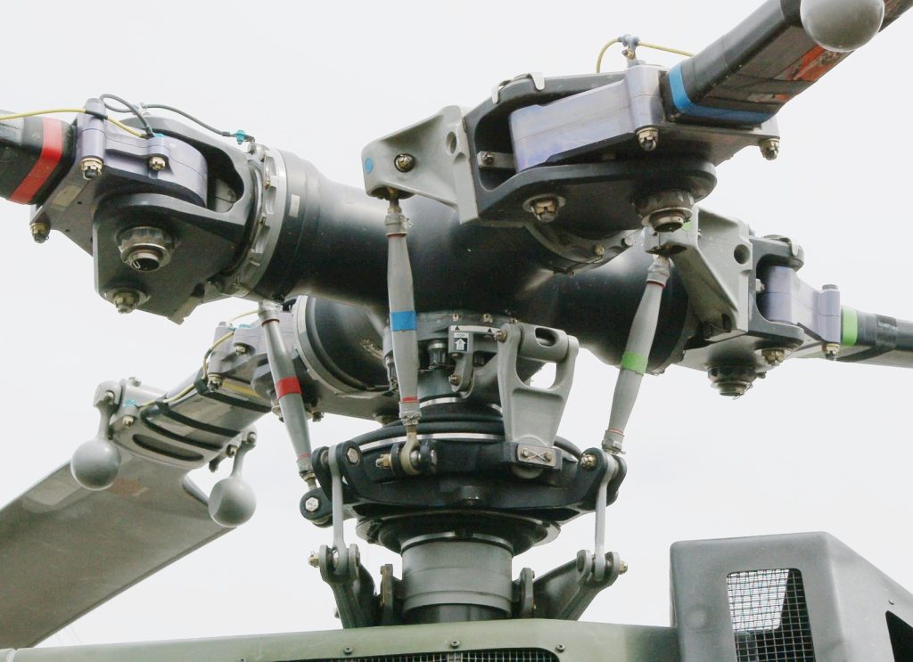
The inputs produced by the swashplate consist of the average or collective pitch and the lateral cyclic,  , and the longitudinal cyclic,
  , i.e.,
(325) 
The collective pitch, , controls the average pitch and the total rotor thrust. The cyclic pitch controls the orientation or tilt of the rotor disk and the direction of the rotor thrust vector. The blade pitch motion itself is induced through a pitch or feathering bearing. A pitch horn is attached to the blade outboard of the pitch bearing. A pitch link is connected to the pitch horn and the upper (rotating) part of the swashplate so that as the upper plate rotates, the vertical displacement of the pitch link produces blade pitch motion.
The novel part of the helicopter swashplate is its ability to tilt to an arbitrary orientation, which requires a gimbal or spherical bearing between the swashplate and the rotor shaft. This mechanism allows a first harmonic blade-pitch input with any phase angle. The upshot is that the rotor disk plane can be tilted to any orientation in space, as illustrated in the schematic below.
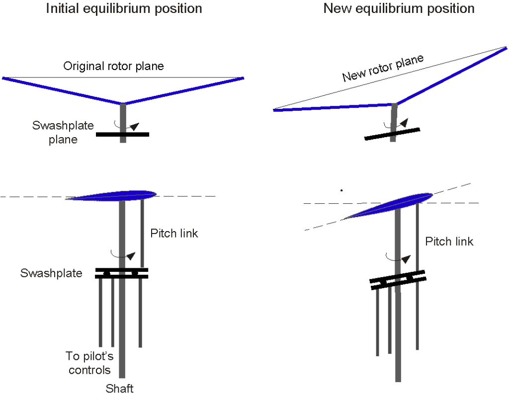
The two figures below explain the relationship between blade pitch (and lift) and blade flapping displacements. Imposing pitch changes other than once per revolution for flight control is unnecessary. Again, the blade pitch (or feathering) motion imposed by the swashplate is described by
(326)
remembering that the imposed (controlled) value of modulates the value of the rotor thrust.
The first harmonic blade of the blade flapping response is given by
(327) 
The mean value, , is called the coning angle, which results from a balance of the moment of the blade lift and the centrifugal force about the flapping hinge.
For and inputs then the blade flapping response will be
(328) 
Notice that because of the dynamic behavior of the blade, the flapping response lags the blade pitch (aerodynamic) inputs by  or 90.
Therefore, if the swashplate produces a once-per-revolution aerodynamic forcing, the rotor blades will flap once per revolution, and the rotor disk plane will then precess to a new orientation in space, thereby tilting the thrust vector. The system is fundamentally straightforward; an aerodynamic forcing is applied at (or close to the natural frequency of the flapping blade, and the blades then respond so that one unit of cyclic pitch input results in (almost) one unit of flapping response. This behavior is strictly applicable to a rotor with a flapping hinge at the rotational axis; even with a hinge offset, the underlying physics and rotor response remain essentially the same.
The figure below illustrates more clearly what happens with a blade pitch input (longitudinal cyclic) from the swashplate, which means that the blade lift will be phased around the rotor disk such that it will reach a maximum at  and a minimum at
  . Because of the 90 phase lag between the generation of lift and the blade flapping response, in this case, the blades will flap up and reach a maximum displacement at
  and a minimum displacement at
  , the net effect, being that the rotor disk plane will tilt backward.
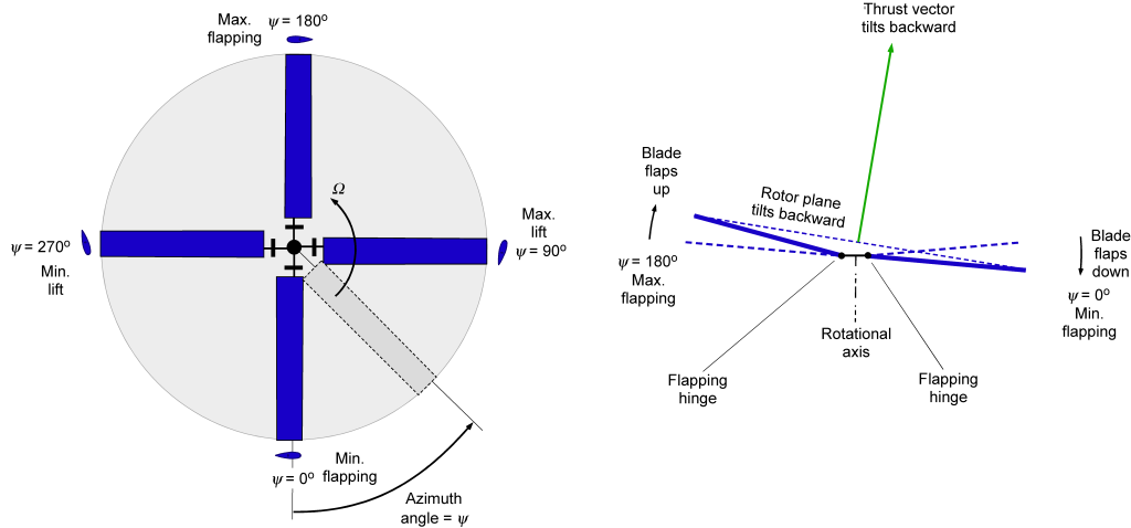
The second figure, as shown below, illustrates what happens with a blade pitch input (lateral cyclic) from the swashplate, which means that the blade lift will be phased around the rotor disk such that it will reach a maximum at and a minimum at . Again, because of the 90 phase lag between the generation of lift and the blade flapping response, the blades, in this case, will flap up and reach a maximum displacement at and a minimum displacement at , the net effect is that the rotor disk plane will tilt to the left (to port) when viewed from behind. The mystery of controlling the helicopter is now solved!
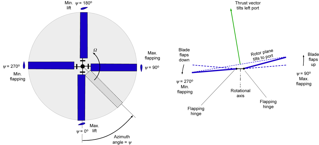
Tail Rotors
The primary purpose of the tail rotor is to provide a sideward force on the airframe in a direction of sufficient magnitude to counter the main rotor torque reaction. If the distance from the main rotor shaft to the tail rotor shaft is , the tail rotor thrust required will be
(329) 
where is the angular velocity of the main rotor. This latter equation assumes no interference or off-loading of the tail rotor by the fin in hover or forward flight.
The second purpose of the tail rotor is to provide directional (yaw) control by modulating its thrust. The pilot controls thrust by pushing on a set of floor-mounted pedals, similar to the rudder pedals on an airplane. For example, if the rotor turns in the conventional direction (counterclockwise when viewed from above), pushing on the left pedal increases the tail rotor thrust (positive to starboard), and the helicopter will yaw nose-left about its center of gravity.
As for the main rotor, the power required to drive the tail rotor depends on the disk loading. A larger diameter may be preferable for low-induced power requirements, but several factors outweigh this choice. First, a larger diameter typically indicates a heavier design, which is undesirable due to its adverse effects on the helicopter’s center of gravity. Second, to meet certification requirements, the tail rotor disk loading and induced velocities are usually set high enough to prevent the tail rotor from entering the vortex ring state (VRS) during sideward flight. These constraints dictate the use of a relatively small tail rotor with high disk loading.
Types of Tail Rotors
Tail rotors may be either of the pusher or tractor variety, as shown in the figure below, and can be located on the left or right-hand side of the vertical fin. All designs suffer from interference between the rotor and the fin, to varying degrees, depending on the tail rotor size or disk area, the fin area, and the spacing between the tail rotor plane and the fin. Canted fins attempt to minimize tail rotor/fin aerodynamic interference. Canted tail rotors can generate vertical thrust and a pitching moment on the fuselage, widening the helicopter’s allowable center of gravity envelope.
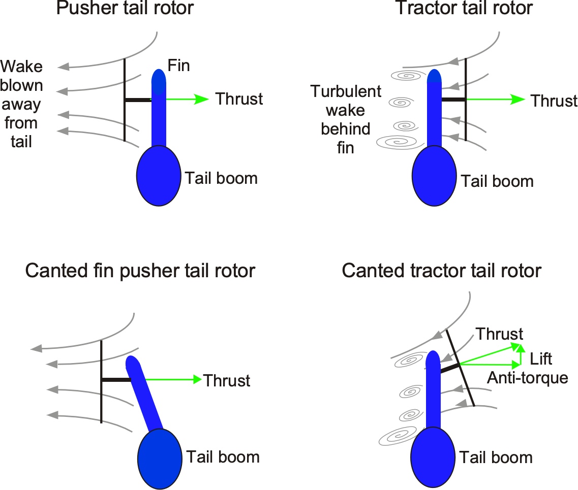
In contrast, the tractor-tail rotor design features a vertical fin located within the high-energy region of the tail rotor wake. While this “blockage” effect tends to increase the tail rotor thrust, a significant force is also applied to the vertical tail that is in the opposite direction to the anti-torque thrust requirement. It is found, however, that the net effect is a decrease in thrust compared to what would be obtained if the rotor were operating in isolation. The interference effects become more significant in both cases with larger fins and smaller rotors. As a result, most modern helicopters use a pusher tail rotor design because this configuration tends to have a higher overall anti-torque-producing efficiency.
Other Effects
A secondary effect of the anti-torque side force is the tendency for the helicopter to drift sideways. This effect is corrected by the main rotor, which is slightly tilted to the left (via cyclic pitch inputs) so that a component of the main rotor thrust produces an equal and opposite side force. This behavior is why a helicopter will tend to hover with one wheel (or skid) lower than the other. On larger helicopters, the main rotor shaft is physically tilted slightly (as part of the design), thereby introducing a pretilt, so the pilot requires less cyclic pitch input to counter the tail rotor side force. The tail rotor thrust and the main rotor side force component act together, producing a couple and a rolling moment about the center of gravity (c.g.). To minimize this moment, the tail rotor is mounted vertically on the tail structure, ensuring the thrust vector’s line of action is close to the helicopter’s center of gravity.
The tail rotor must also provide the specified yaw acceleration in the maximum specified crosswind conditions, accounting for possible efficiency losses due to aerodynamic interference between the tail rotor and the vertical fin. Furthermore, when the main rotor thrust or power is increased, for example, to climb, the reaction torque on the fuselage is increased. This effect means the tail rotor thrust must also increase to balance this torque reaction. Therefore, when the pilot raises the collective pitch to climb, foot pressure must be applied to the appropriate pedal to keep the nose pointed straight in the desired direction of flight.
Design Features
Tail rotors typically have two or four blades, with no particular aerodynamic advantage to either configuration. Only a collective pitch is required because there is no need to control the orientation of the tail rotor disk plane. Tail rotor blades may have some built-in twist to help minimize induced power requirements. Although some blade designs may use cambered airfoils, the tail rotor blades on many helicopters typically employ symmetric airfoils because of their excellent overall performance, reduced pitching moments, and the ability to work equally well at both positive and negative angles of attack. Generally, tail rotors are designed to operate at tip speeds comparable to those of the main rotor. Lower tip speeds are desirable to minimize noise. However, tail rotors operating at lower tip speeds require higher solidity to prevent blade stall for a given thrust. A lower tip speed also increases the torque requirement. Both of these factors will increase the weight of the drive system.
Common to all tail rotors is the lack of cyclic pitch; only collective pitch is used, as control of the tail rotor disk orientation is not required. Nevertheless, the tail rotor must be equipped with flapping hinges to allow the blades to respond to changing aerodynamic conditions. Lead/lag hinges are not usually used to save weight and reduce mechanical complexity. Instead, pitch/flap coupling is built into the tail rotor design, as shown in the photograph below. In this case, the coupling is introduced by locating the pitch horn 45 in front of the blade feathering axis. This approach enables the blades to pitch cyclically, minimizing blade flapping caused by the changing aerodynamic loads during forward flight.
Autorotation
All aircraft must be able to land safely in the event of a complete power failure; this is a certification requirement for civil aircraft and an acceptance criterion for military aircraft. Helicopters are no exception. Loss of power in a helicopter can result from a mechanical problem with the main rotor or gearbox, tail rotor failure, other related tail rotor-drive issues, or even fuel starvation (yes, it does happen). Autorotation is a high-performance maneuver used to land a helicopter in the event of power failure; it establishes a flight condition equivalent to gliding in an airplane. Unfortunately, a helicopter is not a good glider, partly because of its relatively low lift-to-drag ratio. However, a well-trained helicopter pilot should be able to conduct a safe autorotational landing after losing power.
Autorotation is a rapidly descending flight condition during which the upward flow through the rotor produces in-plane aerodynamic forces that create a net torque to drive the rotor, i.e., the rotor self-rotates because it absorbs power from the relative airstream rather than requiring power delivered at the shaft from the engine, as shown in the figure below. Underlying this behavior is the principle of conservation of energy. Because of the upward flow through the rotor, the lift vectors at some points over the blades are tilted forward rather than backward, driving the rotor, resulting in a zero-torque descending flight condition.
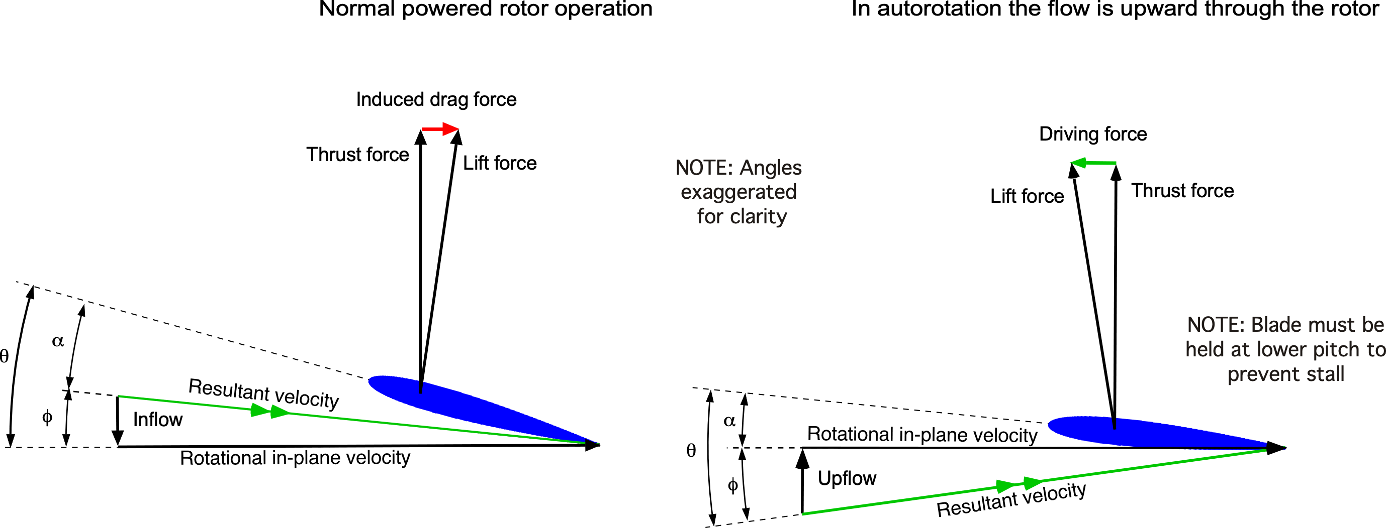
Energy Analysis
Under established, steady autorotative conditions at a constant airspeed, there is an energy balance in which the decrease in aircraft potential energy per unit time equals the power required to sustain the rotor speed and produce thrust and control. In other words, the pilot gives up altitude at a controlled rate in exchange for available energy to continue turning the rotor and maintain thrust.
In general, the instantaneous energy state of the helicopter, , can be written as the sum of its potential energy (altitude),  , translational kinetic energy (airspeed),
  , and stored rotor energy (rotor rotational speed),
  , i.e.,
(330) 
where is the weight of the helicopter,  is the height above ground level (AGL), is the true airspeed,
  is the rotor’s polar moment of inertia, and is the rotor’s angular velocity.
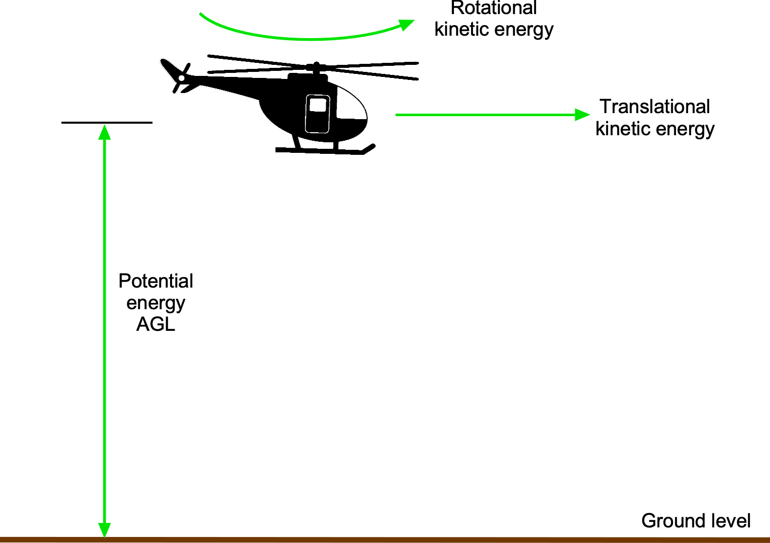
Differentiating Eq. 330 with respect to time gives
(331) 
The time rate of change of energy is power, so Eq. 331 represents a power available equation from a given energy state that could be used to drive the rotor in the event of engine power loss, i.e., to make up for the engine power loss. Notice that  is a rate of altitude change relative to the ground with respect to time, i.e., a rate of descent.
In autorotation, this initial energy must be dissipated at a controlled rate to produce the power to drive the rotor; this means that  is negative. If the initial energy state is
  , then at any subsequent time
  , the energy state will be
(332) 
(333) 
The initial energy state can be expressed as
(334) 
where  is the initial height AGL,
  is the initial airspeed, and
  is the normal rotor speed. Equation 333 can also be written as
(335) 
where  is the rate of descent of the helicopter. Notice that in a decent, is negative, i.e.,
  .
.
All three energy elements in Eq. 335 could, in principle, be used to drive the rotor and sustain autorotational flight after the complete loss of power to the rotor:
- Give up altitude, i.e., potential energy.
- Decrease airspeed, i.e., give up translational kinetic energy.
- Decrease the rotor speed, i.e., release stored rotor energy.
It would be undesirable, at least initially, to use rotor energy (i.e., rotor speed) because the rotor must maintain thrust and allow for control. Indeed, the ability to use the stored rotor energy will be limited by the lowest allowable rotor speed,  , such that
(336) 
where is the normal rotor speed. Usually  is about 80% of , but it depends on the helicopter.
However, as will become increasingly apparent in the following discussion, the ability to perform a successful autorotation to the ground ultimately requires the pilot to utilize all three available energy sources, ensuring that the helicopter’s net energy state at the end of the autorotation is approximately zero. This goal becomes an energy management problem related to the flight trajectory, which, in turn, requires the pilot to properly use the flight controls.
Autorotative Rate of Descent
Assume a constant airspeed and rotor speed, then for a given weight, , then
(337) 
This result shows that the pilot must descend at a sufficiently high rate to continue supplying power to drive the rotor, i.e., give up altitude or potential energy at just the correct rate from the initial energy state after power loss. Potential energy (altitude) is by far the most significant energy source, so giving up altitude is a necessary condition for an autorotation to occur.
Vertical Autorotation
In the zero-airspeed condition, i.e., a pure vertical autorotation, it has been previously shown that the equilibrium condition is achieved when
(338) 
which, as previously shown, occurs under the condition
(339) 
when including the profile power contribution, . Therefore,
(340) 
It is assumed that thrust equals weight, i.e.,  . Notice that the rate of the autorotative descent increases with the square root of disk loading, , i.e., increasing the helicopter’s weight, and with increasing density altitude, i.e., lower air density. It is found that the helicopter’s autorotational rate of descent is relatively high and much higher than what could be sustained to the ground, an issue discussed later.
Autorotation in Forward Flight
In forward flight, the power required for flight can be approximated as
(341) 
where the induced velocity, , is given by Glauert’s approximation, i.e.,
(342) 
which is valid for higher airspeed values, , and is almost independent of the rate of climb or descent, . During autorotative forward flight, the rotor does not operate in the VRS or turbulent wake state, so the induced velocity is predictable according to momentum theory. For a given helicopter, variations of profile power, , and parasitic power, , depend mainly on airspeed and can also be assumed independent of the rate of climb or descent. In an established autorotative descent, then
(343) 
where  is the power required for level flight at the same weight, density, altitude, and airspeed. Therefore, in the autorotative state in forward flight at a constant airspeed, the power to drive the rotor comes by giving up altitude at a controlled rate, i.e.,
(344) 
as shown in the figure below.
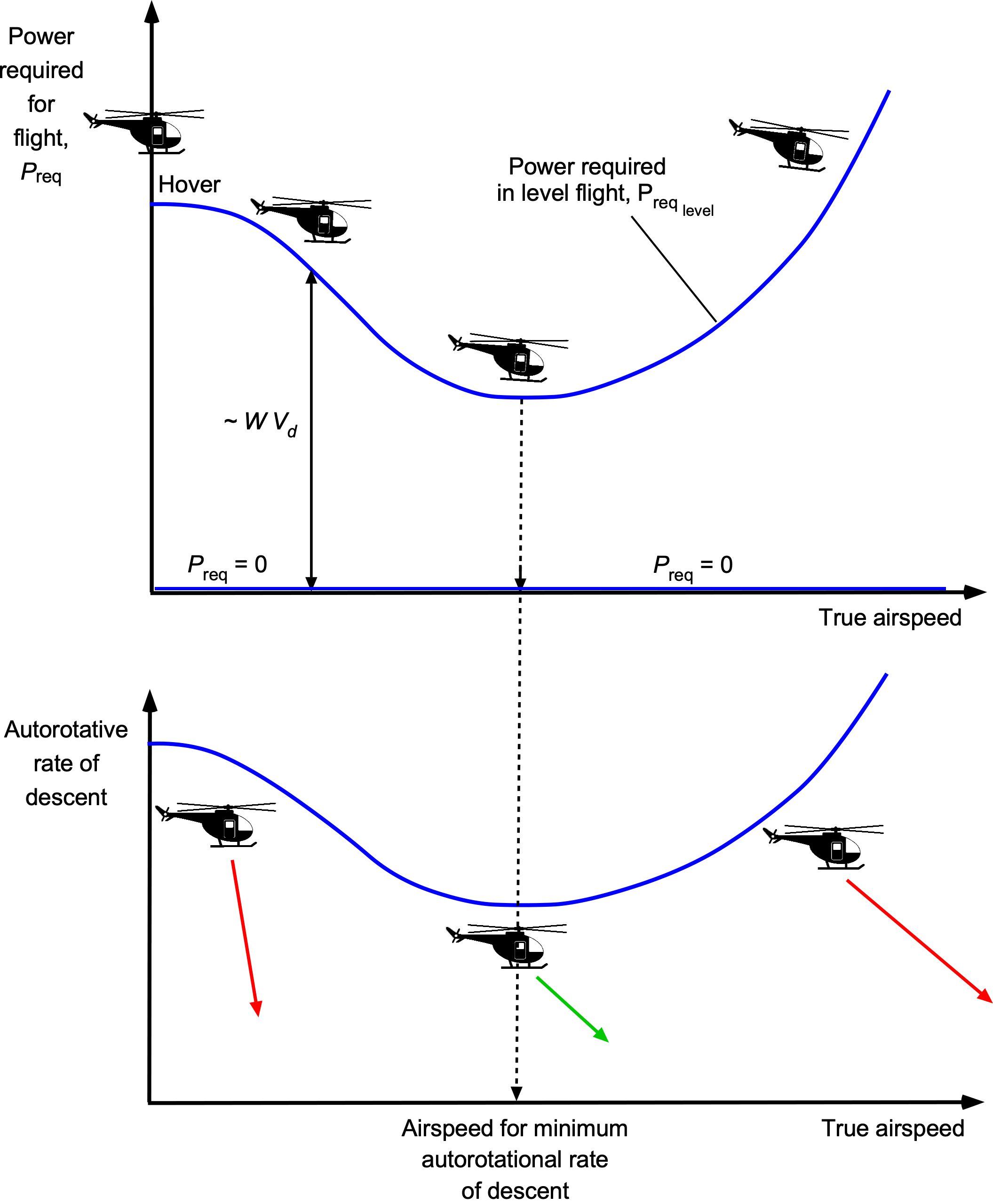
It will now be apparent that the autorotative descent rate depends on the airspeed at which the helicopter is flying. The highest rates are achieved at low and higher airspeeds, which should be avoided; a minimum rate of descent is obtained at an intermediate airspeed. However, the descent rates of an autorotating helicopter remain high at all airspeeds and cannot be sustained as the helicopter approaches the ground.
Assume that some excess translational kinetic energy is also available at a constant autorotative descent rate. In this case, then
(345) 
Notice that the term  is a deceleration, which must be relatively quick to extract much energy. However, there are two conditions where airspeed can (or should) be used to control the flight path during the autorotational maneuver. The first is achieved by pitching to obtain the lowest descent rate during autorotation. The second is near the ground, where any remaining kinetic energy can help arrest the descent rate and reduce airspeed.
Finally, the potential effects of rotor speed on autorotational characteristics must be considered. The rotor speed must be maintained throughout the maneuver because the rotor must maintain thrust, provide sufficient control, and avoid excessive blade flapping (due to reduced centrifugal forces). It is also essential to be aware that if the rotor speed decreases too much, the pilot may lose sufficient control over energy management during the landing phase.
The safe rotor speed range in autorotation for most helicopters is usually between 80% and 120% of the normal rotor speed, , which the pilot controls using collective pitch. If the rotor speed drops too low, the rotor will begin to stall, and excessive blade flapping may occur due to reduced centrifugal force on the blades. There is also a risk that excessive flapping could cause the blades to contact the airframe. Conversely, structural overloads become a concern if the rotor speed becomes too high.
Summary of the Autorotational Maneuver
It is now possible to combine the elements of energy management to describe the ideal autorotational maneuver, as summarized in the figure below. A successful autorotational maneuver to the ground requires a high level of piloting skill, especially in larger, heavier helicopters.
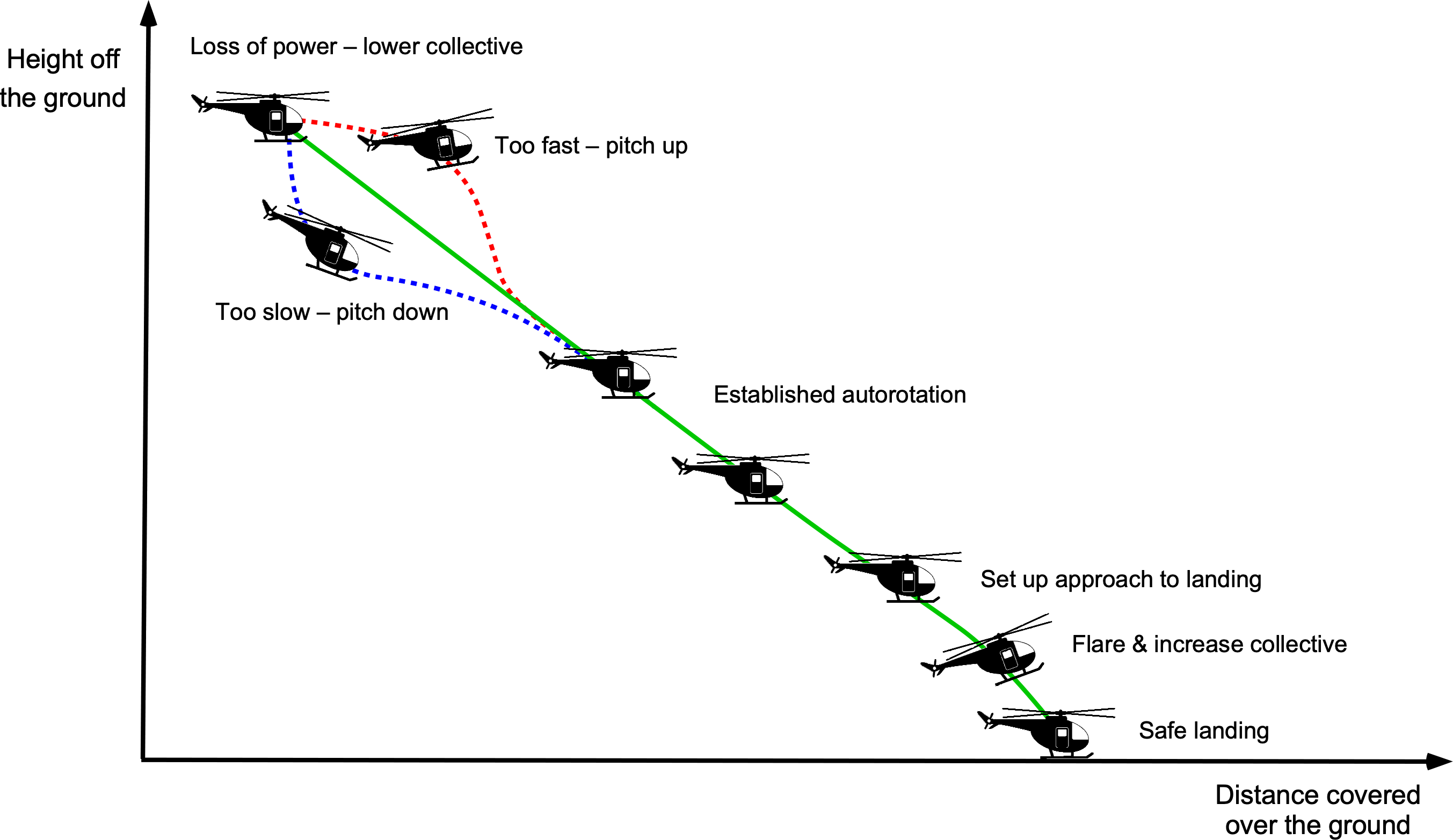
Generally, a helicopter rotor’s polar moment of inertia is such that rotor speed can decay quickly, and some decrease in rotor speed can be anticipated upon entry into an autorotation, unless a sufficiently low collective pitch is used to achieve steady-state autorotation. However, there may be aerodynamic and structural limits such as rotor stall, collective and cyclic pitch limits, and allowable blade flapping. The pilot must also be aware that if the collective is set too low, it can cause rotor overspeed during autorotation. In any case, the pilot’s first reaction to a complete loss of power is to immediately reduce the collective pitch to reduce drag on the blades and maintain rotor speed.
In established autorotation, judicious control of the rate of descent and flight path will allow the pilot time to determine a suitable landing location. Any excess airspeed can be used to slow the autorotative descent rate closer to the lowest value. Bleeding off excess airspeed is performed by pulling back on the cyclic for a few seconds, also lowering the descent rate. If the airspeed is too low, forward cyclic can be used to reach this airspeed at the expense of some potential energy, i.e., some additional altitude loss. Most helicopters typically have the best autorotative rate of descent at an airspeed between 60 and 80 knots.
Near the ground, when the potential energy is essentially depleted, the stored rotor energy and any remaining kinetic energy can be used to arrest and cushion the final landing. This is achieved by the pilot pulling up on the collective, which increases thrust but causes the rotor speed to decay. Pitching up to a nose-high attitude will extract any remaining translational kinetic energy, helping maintain rotor speed while preventing the tail from striking the ground. This type of maneuver before the final landing is common to all autorotations. The overall objective of the pilot is to cushion the rate of descent so that the helicopter touches down at a rate of descent less than about 10 ft s (h 3 ms) with minimal forward speed.
Suppose the pilot manages the controls and flight trajectory such that all initial potential, kinetic, and rotational energy is fully converted to kinetic energy at the end of the autorotational maneuver. In that case, the helicopter comes to rest on the ground with zero airspeed and a lower-than-normal rotor speed. Some residual rotor speed is desirable to maintain directional control (through the tail rotor inputs) and minimize blade flapping as the helicopter settles onto the ground.
Rotor Design for Autorotational Capability
A primary aspect of the rotor design that must be considered in assessing the autorotational behavior of the helicopter is its polar moment of inertia and its stored rotational kinetic energy. There are two design points to consider: 1. The potential decay in rotor speed after the initial loss of power. 2. The stored kinetic energy of the rotor system at the end of the autorotational flight maneuver can be utilized to arrest the descent rate, allowing the helicopter to land safely. Both conditions involve the rotor’s polar moment of inertia.
The equation describing the decay of the rotor’s rotational speed is
(346) 
where is the torque to the rotors shaft, and is the initial or normal rotor speed. Integrating Eq. 346 using separation of variables gives
(347) 
where the subscript 0 refers to time  . After rearrangement, then
(348) 
(349) 
This outcome means that rotors with higher levels of stored kinetic energy and lower power requirements (i.e., the lowest disk loading) will have the largest values of  , resulting in the slowest rate of rotational speed decay after power loss. For a given rotor speed, the rotor inertia controls the kinetic energy, which must have a minimum value for the helicopter to meet autorotational safety requirements, posing a design problem.
Initial Energy State (Height-Velocity Diagram)
The acceptable flight conditions and, hence, the initial energy state, , that allow for the recovery of the helicopter and safe entry into autorotation are summarized for the pilot as height-velocity (H-V) curves. The initial energy state can be expressed as
(350) 
where is the initial height, is the initial airspeed, and is the normal rotor speed. The potential and kinetic energy are sufficient for the pilot to land safely using autorotation anywhere outside the AVOID region. Inside the avoidance region, the initial energy state is too low to perform a successful autorotation to the ground. While flight in the AVOID region is not otherwise prohibited, its boundaries define the conditions under which sustained flight operations should be avoided. Some margin for pilot reaction time, which may be several seconds, must also be allowed to determine these boundaries, increasing the H-V diagram’s vertical and horizontal extent.
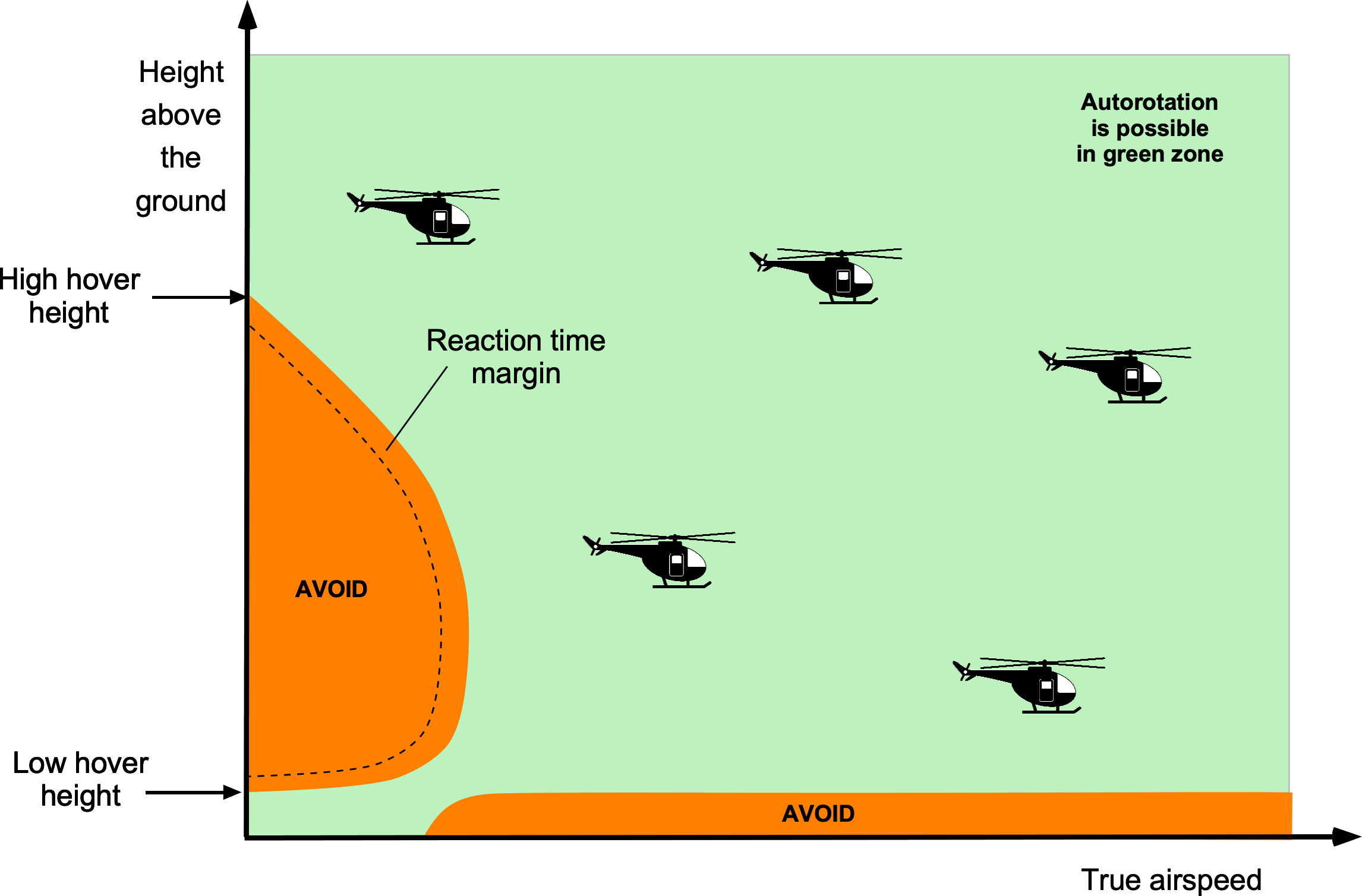
The size and shape of the H-V curve depend on several factors, including the helicopter’s general characteristics, its gross weight, and operational density altitude. The disk loading is the primary parameter influencing the autorotative rate of descent and the extent of the AVOID region. Note that the H-V diagram defines two AVOID regions. The second AVOID region, characterized by lower altitudes and higher airspeeds, determines the minimum altitude below which translational kinetic energy cannot be converted into potential energy through a zoom-climb before entering autorotation. The most critical AVOID region, however, is at low airspeeds.
Reducing the size of the AVOID region is desirable from an operational perspective, but it often requires more engineering effort. Helicopters with low disk loading tend to have smaller AVOID regions; hence, the need for safe autorotative characteristics must be considered in the basic sizing and design of the rotor system. In this regard, the higher the polar moment of inertia, the smaller the AVOID region. The downside is that reducing a rotor’s disk loading and increasing its polar moment of inertia results in a larger, heavier rotor, reducing the helicopter’s useful load.
A survey of helicopter accidents conducted by Harris et al. found that 2,408 of 8,436 accidents were caused by engine power loss. Approximately half of these 2,408 accidents were caused by fuel exhaustion; 935 resulted in substantial damage to the helicopters, and 445 helicopters were destroyed. Besides the tragic loss of lives, such statistics are certainly not acceptable from an engineering standpoint and clearly emphasize the need for better helicopter designs with adequate single-engine inoperative performance and safe autorotational landing capability.
Autorotative Index
As will now be apparent, the autorotative performance of a helicopter depends on several factors. These include the rotor disk loading and the stored kinetic energy in the rotor system. Part of the issue is the subjective “difficulty rating” assessments by test pilots. Therefore, an autorotative index is often used to aid in rotor design. Although various indices have been used, the autorotation index is a rotational kinetic energy factor. One autorotative index,  , is given by
(351) 
where would be the maximum gross weight and , is the corresponding disk loading.
Autorotative indices for several helicopters at standard sea-level conditions based on published information for each helicopter are shown in the figure below. These indices are helpful in rotor sizing or examining the effects of autorotative characteristics with increasing gross weight or density altitude. The absolute values of the index are not significant. Still, the relative values provide a means of comparing the autorotative performance of new designs with that of designs already having acceptable autorotative characteristics. An index of about 20 is generally adequate for single-engine helicopters. In contrast, a multi-engine helicopter can have an index as low as 10 and still maintain safe flight characteristics in the event of a single-engine failure.
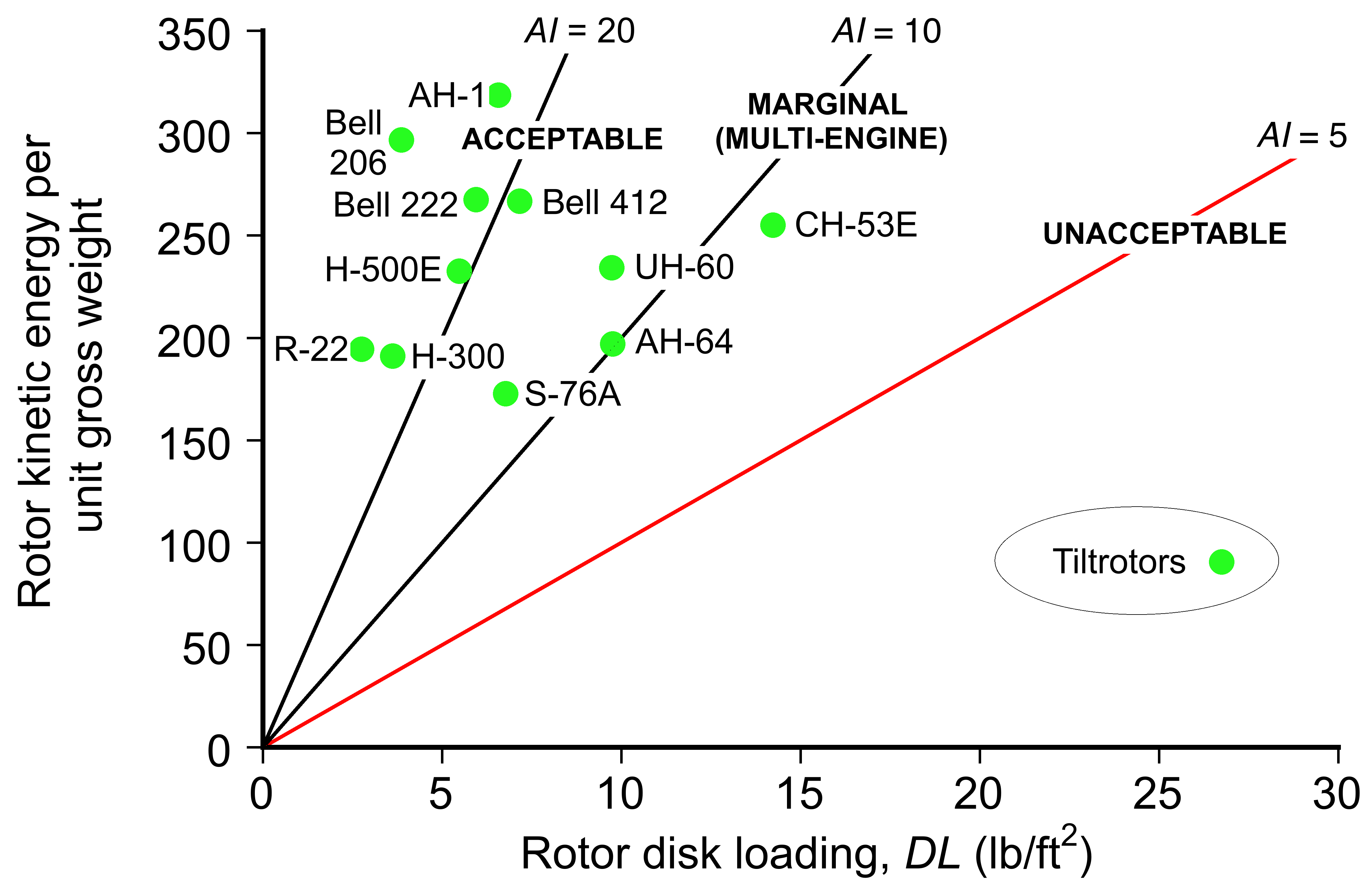
Limitations of the Helicopter
Helicopters are versatile aircraft with unique capabilities, but like all aircraft, they have intrinsic limitations. As summarized in the figure below, the helicopter suffers from a fascinating concatenation of aerodynamic and aeromechanical problems that limit its overall capabilities, especially as it flies faster. Airplanes are limited by the onset of wing stall at low airspeeds and compressibility at high airspeeds. Either or both can limit a helicopter’s performance at the same airspeed! Remember that for a helicopter, however, “fast” means only about 150 kts (278 kph). As previously discussed, helicopters are less aerodynamically efficient than fixed-wing aircraft, so their flight range and payload are limited. The creation of obtrusive noise is also a concern for helicopters in both civil and military use.
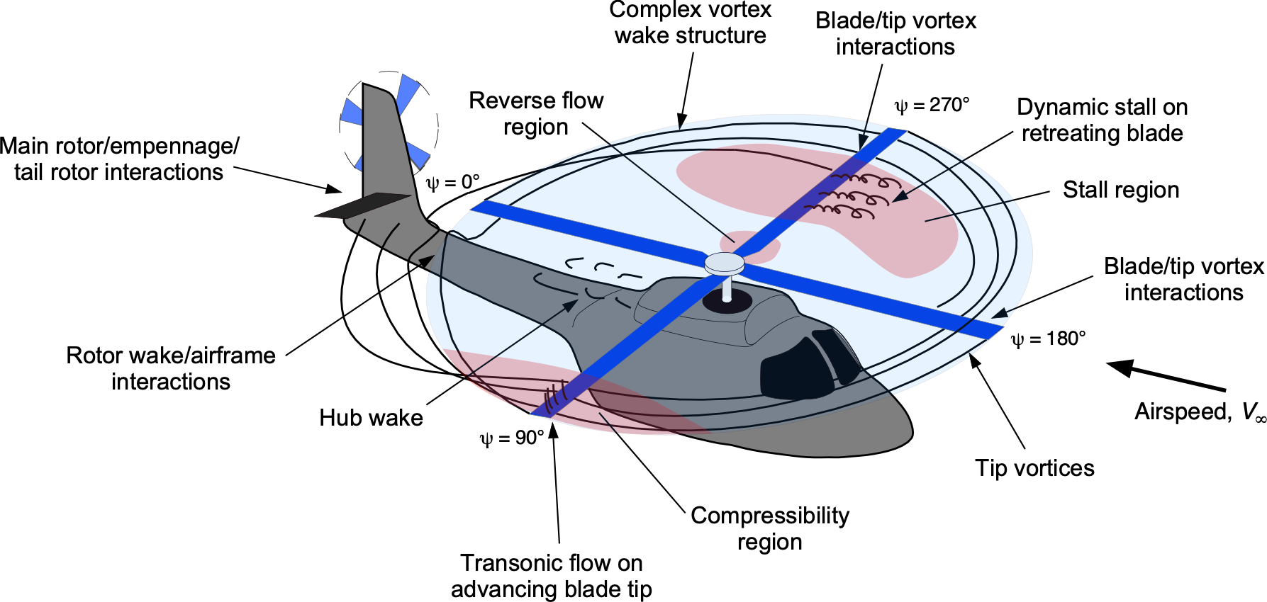
Advancing Blade Compressibility
The most apparent aerodynamic effect limiting the forward flight performance of a helicopter is that the blade tips on the advancing side of the rotor disk experience compressibility effects at higher airspeeds because of the onset of supercritical and transonic flow. The upshot is the formation of shock waves and the associated wave drag, possibly even shock-induced flow separation. Periodic shock-wave formation can also generate impulsive noise. The increased power demands imposed on the rotor system by compressibility losses can eventually limit the helicopter’s forward flight speed if it reaches its available power or mechanical shaft torque limits.
The onset of compressibility effects on the advancing blade is relatively gradual, increasing with the rotor advance ratio once a critical threshold is reached. Consider the Mach number at the blade tip at = 90o, which is given by
(352) 
Drag from compressibility effects will begin to manifest when  , where
  is the drag divergence Mach number of the airfoil section in the tip region.
The figure below shows that the blade tip can be swept back to relieve these effects, analogous to that used on an airplane wing for high-speed flight. The component of the Mach number normal (perpendicular) to the blade’s leading edge over the tip region is what matters, which will be reduced by  . Therefore, the advance ratio (and hence airspeed) where compressibility effects manifest can be increased (approximately) by a factor of
  before compressibility effects are re-encountered.
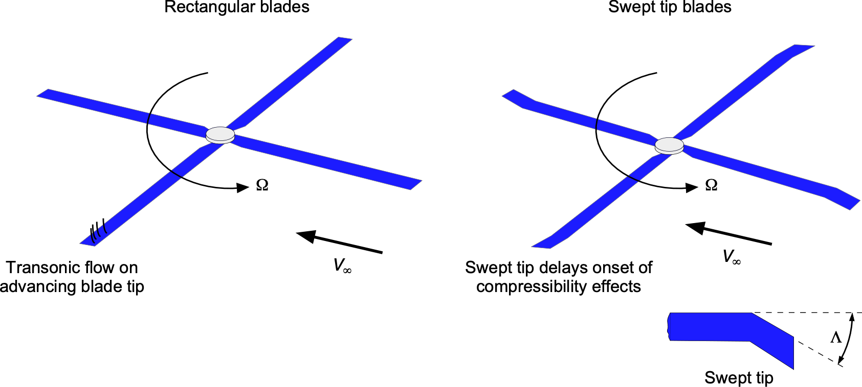
Retreating Blade Stall
On the retreating side of the rotor disk, the local velocities at the blades are relatively low, and the blades must operate at higher angles of attack to maintain lift and propulsion. If these angles of attack become too large, the blades will stall, losing lift and increasing drag, which in turn produces torsional pitching moments that can increase vibratory loads. At higher forward speeds, the onset of reverse flow on the retreating blade contributes to a loss of lift and higher drag. Both stall and reverse-flow effects result in a loss of overall lifting and propulsive capability from the rotor, and, like compressibility effects, they form an aerodynamic limit that impedes further increases in forward flight speed or the rotor’s ability to carry more weight at a given flight speed.
Because the flow environment on rotor blades in forward flight is inherently unsteady, combined with the pitch rates resulting from cyclic pitch inputs and torsional blade dynamics, blade stall is referred to as dynamic stall. This phenomenon has attracted considerable research interest due to the unsteady aerodynamic effects it produces, including the shedding of a leading-edge vortex, as illustrated in the simulation below. The onset of dynamic stall can produce extremely high structural loads and vibrations, thereby limiting the helicopter’s airspeed, load-carrying capability, and maneuvering performance.
Blade/Vortex Interactions
The low rotor disk loading and generally low average inflow velocity through a helicopter rotor keep the blade tip vortices sufficiently close to the rotor, resulting in blade/vortex interaction (BVI). The BVI phenomenon causes sharp changes in blade lift, leading to exceptionally high vibratory loads on the rotor. BVI is also accompanied by significant impulsive noise, a recognizable “wop-wop-wop” signature of an approaching helicopter. The tail rotor (if used) is also a significant source of aerodynamic noise, often manifesting across a wide range of audible frequencies.
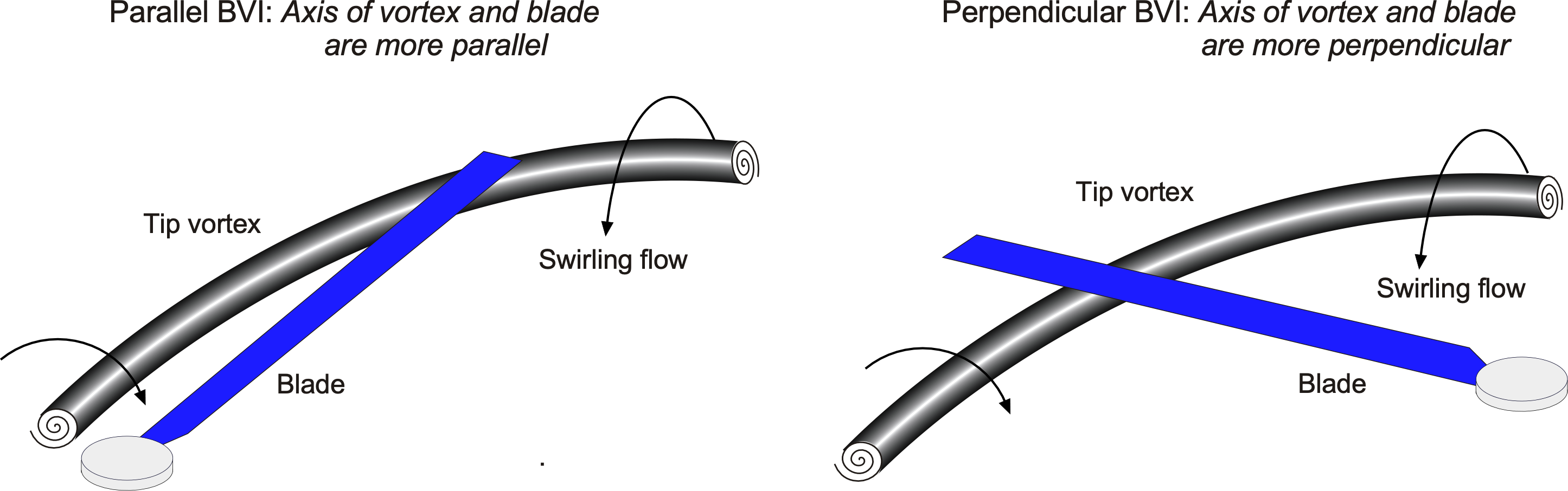
Reducing rotor and engine/transmission noise in the cabin has been a more recent goal in helicopter design. Still, it is essential from both civil (environmental and community acceptance issues) and military (detectability) perspectives. While many mathematical models exist to predict helicopter noise levels, they are primarily grounded in empirical data. Increasingly stringent noise-reduction requirements imposed by certification authorities to develop environmentally friendly aircraft will compel helicopter manufacturers to seek more effective noise-reduction solutions. In most cases, understanding the root of the noise problems on helicopters lies firmly in understanding and predicting their unsteady aerodynamics.
Airframe Aerodynamics
The fuselage of a conventional helicopter is roughly a prolate spheroid, with a cylindrical mast or pylon to support the central rotor hub and controls, and a long, quasi-cylindrical tail boom supporting the tail rotor and empennage, as shown in the figure below. The typically high parasitic drag of these shapes significantly limits the helicopter’s cruise speed, increases its fuel consumption, and reduces its range. In cruise conditions, the primary drag on the helicopter’s airframe is pressure drag; this differs from an airplane’s fuselage, where the dominant drag source in cruise flight is mostly skin friction drag (boundary layer shear stress drag). Most parasitic drag on the helicopter comes from the rotor pylon and hub, the fuselage, engine inlets, the tail rotor, landing gear (skids or wheels), and component flow interference. As for other aircraft types, streamlining can effectively reduce airframe drag, as illustrated in the figure below.
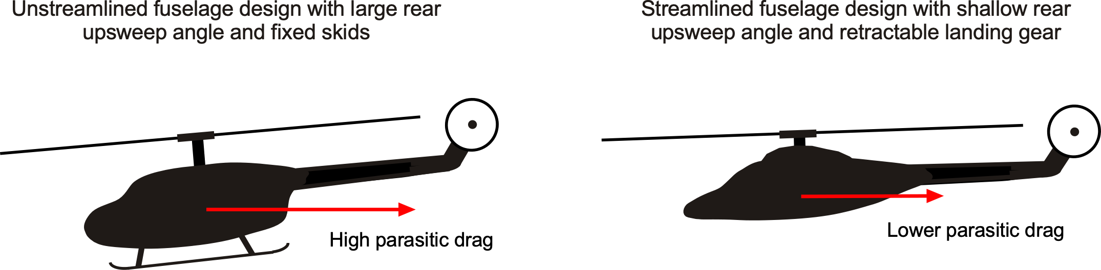
A significant contributor is the fuselage after-body drag, caused by flow separation in the region where the main fuselage tapers to the tail boom. Flow separation forms two energetic trailing vortices on specific fuselage shapes, characterized by high aft taper ratios and large upsweep angles, which further contribute to induced drag. These vortices are not steady, and the subsequent unsteady wake flow can interact with the empennage and tail rotor, increasing vibration levels and producing tail shake.
The exposed rotor pylon, hub, and blade attachments significantly contribute to airframe drag and are another source of unsteady flow or buffeting. As expected, the rotor hub has a significant impact on drag and the helicopter’s forward flight performance. However, minimizing the rotor mast height and enclosing the swashplate and pitch linkages inside a fairing helps reduce this parasitic drag.
Future Helicopters?
The schematic below illustrates one hypothetical future or ultimate helicopter concept incorporating a melange of technological ideas. This does not mean that future helicopters will look like this, and almost certainly not because such an aircraft would be prohibitively expensive to develop; instead, it simply means that they will incorporate one or more of the concepts synthesized in this schematic. However, it’s essential to realize that developing and adopting new technologies in the helicopter industry is a gradual, if not incremental, process. Therefore, future helicopter design changes will be driven not only by technological advancements but also by regulatory considerations, reliability, environmental concerns, costs, and other requirements.
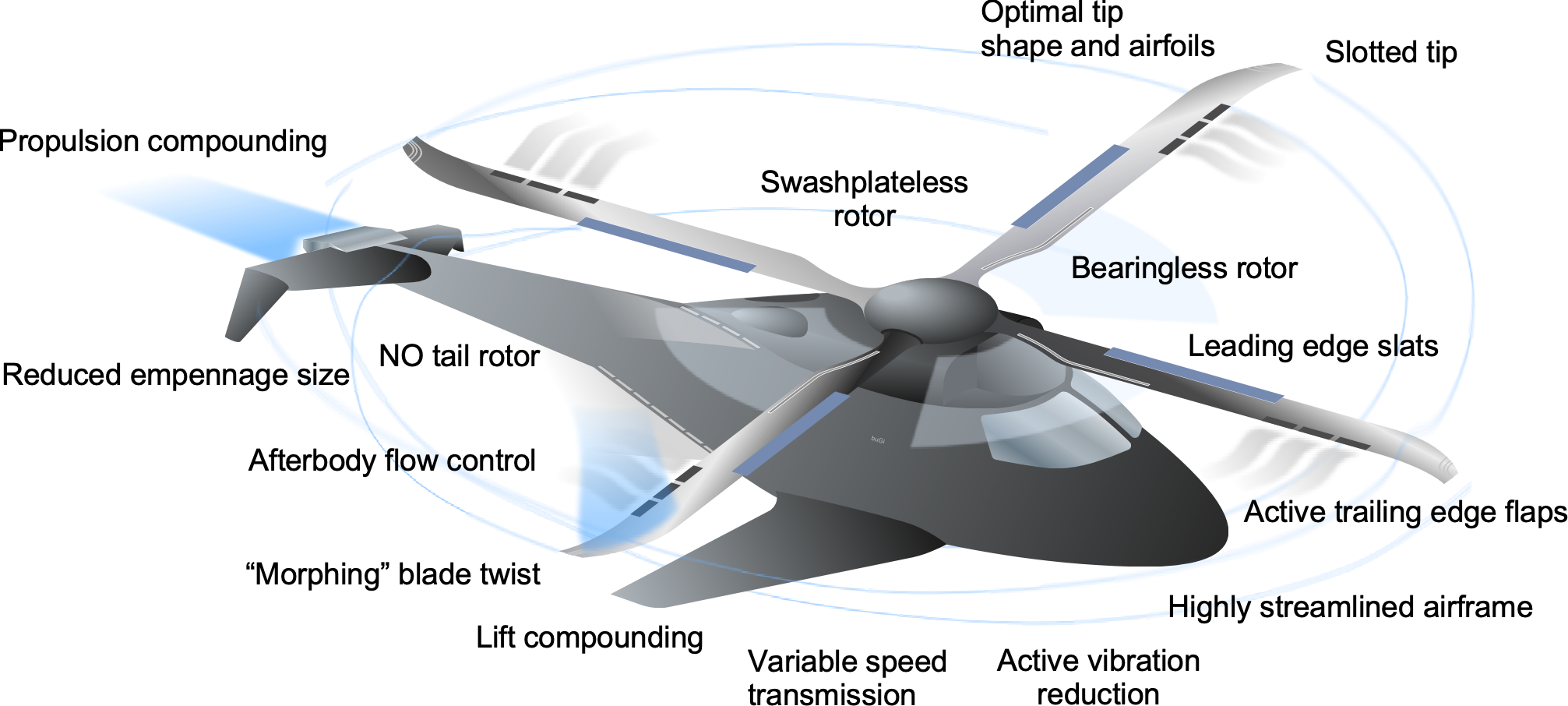
Future helicopter designs will continue to incorporate state-of-the-art materials and design techniques to enhance aerodynamics and reduce structural weight, thereby improving fuel efficiency and overall performance. Helicopters might adopt more modular designs, allowing for easier customization and upgrades. This could make it cost-effective to have helicopters with mission-adaptive profiles, i.e., by swapping out modules or components for different missions. Future helicopters, at least the smaller ones, will incorporate hybrid or fully electric propulsion systems to reduce emissions and noise, making them more sustainable and less disruptive. However, in the end, the ultimate helicopter may be a relatively simple but extremely well-designed machine with as few of these “gadgets” as possible.
The future seems clear. On the one hand, the traditional helicopter industry, much like aerospace as a whole, tends to favor reliability and incremental improvements over innovation. This is understandable because safety regulations, high R & D costs, and the long lifecycle of aircraft contribute to this conservatism. However, it appears that the existing industry is destined for stagnation. On the other hand, startup companies have the flexibility to explore new technologies, such as electric propulsion, autonomous flight, or novel airframe designs, without being weighed down by the need to conform to legacy systems and corporate bureaucracy. New companies are already pushing the envelope with eVTOL (electric vertical takeoff and landing) aircraft, which could disrupt traditional rotorcraft operations.
Summary & Closure
The factors governing the performance and behavior of helicopters have now been examined in detail. Beginning with the simple actuator-disk model, momentum theory was used to establish the fundamental limits of rotor performance in hover, climb, descent, and forward flight. Central to these limits is the disk loading: low disk loadings reduce induced power and directly improve hovering efficiency. Complementary performance metrics such as power loading and figure of merit were introduced to compare rotor systems and assess their aerodynamic effectiveness. The basic momentum model was then refined to incorporate non-ideal effects, bringing theoretical predictions into closer alignment with measured rotor performance.
The framework was extended to more complex configurations, including coaxial rotors, where the mutual interference of the two rotor wakes modifies induced power. In forward flight, the inherently nonuniform inflow requires numerical solution methods to determine the induced velocity distribution across the disk. These analyses lead naturally to the principal performance characteristics and limitations of helicopters in forward flight, including the factors that constrain maximum speed and influence overall efficiency. Together, these results form the foundation for understanding the aerodynamic performance of helicopter rotors and for evaluating the tradeoffs that shape rotorcraft design.
5-Question Self-Assessment Quickquiz
For Further Thought or Discussion
- The history of airplanes shows that growth (in the number of prototypes under development) was rapid and monotonic. However, while the evolution of rotorcraft (helicopters) began earlier, it progressed in a series of discrete events, marked by “fits and starts.” Discuss this point further, assuming it is associated with technological developments.
- Briefly overview the leading technical problems encountered when building and flying a helicopter before 1900. In your discussion, consider overall levels of aeronautical knowledge, stability and control requirements, the availability of suitable engines, construction materials, and anything else you feel is relevant.
- Engines are often viewed as one of the most critical enabling technologies for powered flight, especially for helicopters. However, having a readily available supply of suitably formulated and inexpensive fuel for a piston engine (i.e., gasoline) was the critical enabling technology. Discuss this viewpoint.
- Most modern helicopters have a single main rotor and tail rotor (conventional) configurations. For the same overall aircraft gross weight, what might be the relative advantages of using a tandem rotor helicopter over a conventional helicopter? Also, compare the potential relative merits of a coaxial rotor and a side-by-side rotor configuration over a tandem rotor design.
- Discuss the physical and other features distinguishing a helicopter from an autogiro. Discuss also the reasons why the autogiro was quickly eclipsed by the success of the helicopter when it appeared in the mid to late 1930s. Are there prospects for the autogiro or gyroplane in the future?
- Although tiltrotor concepts date back more than sixty years, it is only recently that civilian tiltrotor aircraft have completed much of the flight testing required for civil certification, such as the AW-609. Discuss the technical, economic, and other reasons for this long gestation period. Consider also the prospect that you may fly on a tilt-rotor operated by an airline within the next decade.
- Use conservation of mass and momentum, but use Bernoulli’s equation instead of the general energy equation to prove that the induced velocity in a climbing rotor’s fully contracted wake (slipstream) is twice the induced velocity in the rotor plane.
Other Useful Online Resources
For additional resources on helicopters and other rotorcraft, follow up on some of these online resources:
- Early film. How it Works: Sikorsky H-19 Helicopter.
- History Of Helicopters – Military Helicopter Invention Documentary.
- A great movie on the birth of Bell Helicopters.
- A video showing the details of the swashplate.
- Video on the top 7 U.S. military helicopters of all time!
- Your first helicopter lesson in a Robinson R-44!
- The massive Sikorsky CH-53K helicopter in action!
- Bell 206 JetRanger helicopter review: How to Fly a Helicopter.
- MD 520N NOTAR helicopter review and flight test.
- The author is indebted to his teachers, Professor Alfred Gessow, who was a pioneer in the field of helicopter aerodynamics and co-author of the book "Aerodynamics of the Helicopter," and F. John Perry, Chief Aerodynamicist for Westland Helicopters. ↵
- Juan de la Cierva tragically died in an airplane accident on December 9, 1936. He was a passenger on a KLM Douglas DC-2 that crashed shortly after takeoff from Croydon Airport, London. ↵
- A reasonable assumption in practice, but this particular assumption is still needed to formalize the minimum loss condition. ↵
- Recall that in the ideal case, the performance of the upper rotor is assumed to be unaffected by the lower rotor. ↵
- The power measurements are only accurate to about 7%. ↵
