50 Flight Range & Endurance
Introduction
There are flight profiles and missions in which an airplane must either fly as far as possible (to maximize range) or remain airborne for as long as possible (to maximize endurance). In both cases, the critical factor is fuel availability, that is, the amount of fuel the airplane can carry relative to its rate of consumption. However, the usable fuel load is often limited by tank volume or by the maximum allowable fuel weight. In most airplanes, a trade-off exists between payload capacity (including passengers and cargo) and fuel capacity, as both contribute directly to the airplane’s total takeoff weight.
For example, long-haul commercial flights require a significant nonstop range. Transporting passengers and cargo across the Atlantic Ocean demands a flight range exceeding 3,700 nautical miles (6,850 km). In such cases, range takes priority over endurance. As of February 2025, the longest nonstop commercial flight is Singapore Airlines’ service from Singapore to New York. This route covers approximately 8,300 nautical miles (15,350 km) and is scheduled to take 18 hours and 50 minutes, operated using an Airbus A350-900ULR with a capacity of only 161 passengers. The actual flight range over the ground is also affected by wind, with headwinds reducing range and tailwinds extending it. Maximizing range while flying at high airspeed is essential for minimizing total flight time and requires careful route planning.
Conversely, some flight missions, particularly military operations, prioritize endurance. For example, a surveillance or reconnaissance mission may require an airplane to loiter over a specific area for an extended period. In some scenarios, military aircraft must optimize both range and endurance at different phases of the same mission. A maritime search-and-rescue operation exemplifies this requirement. A good flight range at the highest practical airspeed is needed to reach the search area, while good endurance is crucial for conducting a prolonged search. One example of an aircraft designed for endurance is the P-3K2 Orion, which can remain airborne for more than 15 hours. To conserve fuel, it can shut down two of its four engines during extended patrol operations.
Learning Objectives
- Recognize the role of specific fuel consumption in fuel burn, flight endurance, and range.
- Identify the optimal flight conditions for maximizing range or endurance.
- Apply the appropriate Breguet equations to estimate endurance and range for both propeller and jet aircraft.
- Calculate total fuel burn and interpret payload-range diagrams to assess aircraft performance.
- Understand the effects of airplane aerodynamics and propulsion systems on an airplane’s range and flight speeds.
Fuel Flow & Specific Fuel Consumption (SFC)
Flight range and endurance depend on the amount of fuel that can be carried and the fuel flow rate, which in turn depend on the thrust or power produced by the engine(s) and their other characteristics (e.g., thermodynamic and mechanical). The fuel flow or fuel burn rate is the volume (or, more typically, the mass or weight) of fuel burned by the engine(s) per unit of time. Remember that one metric used to measure an engine’s efficiency is its specific fuel consumption.
BSFC
For engines that deliver power to a shaft, such as those driving a propeller, the SFC is expressed as the power-specific fuel consumption or the “brake” power-specific fuel consumption (BSFC). The BSFC is defined as the weight of fuel burned per unit power produced per unit time of operation, i.e.,
(1) 
When delivering a given amount of power, an engine with a lower BSFC will be more efficient because it burns less fuel per unit of time.
In USC, then  has units of lb bhp
 hr, where “bhp” means “brake horsepower,” so this is the power in hp that can be delivered at the engine’s shaft.[1] In SI units, BSFC is often measured in kg kW hr; remember that in aviation, weight is usually calculated in units of kg although it is strictly a unit of mass; one can convert to Newtons (if needed) by multiplying by acceleration under gravity,
  , where = 9.81 m/s2 = 32.17 ft/s2.
TSFC
In jet engines, SFC is defined as thrust-specific fuel consumption (TSFC). The TSFC is defined as
(2) 
The value of  is also a measure of engine efficiency in converting the energy in the fuel, in this case, into useful thrust; the lower the value of the TSFC, the more efficient the engine. For example, in USC units, the TSFC has units of lb lb hr; in SI units, the TSFC would be measured in units of kg kg hr or just hr.
Notice that the reciprocal of the TSFC is measured in units of time, which is called the specific impulse  . Values of are often given in units of seconds, so the higher the number of seconds, the more efficient the engine is in producing thrust. However, the TSFC is typically used for jet engines, while is used for rocket motors.
Note on fuel weight and the units for TSFC.
Although TSFC can be interpreted to have units of “per hour” (hr) or “per second” (s), it is generally always quoted in units of lb lb hr or kg kg hr. Using the kg as a unit of weight is an anomaly in the SI system that can cause much confusion unless carefully addressed. Nevertheless, in aviation practice, fuel weight is almost always expressed in terms of pounds (lb) or kilograms (kg). Fuel density conversions are critical: Jet-A is about 0.8 kg/L, so 1 t ≈ 1,250 L. For larger quantities, especially in airline operations, the metric tonne (1,000 kg) is commonly used. In the United States, however, fuel weights are typically expressed in pounds, and when the term “ton” is used, it usually refers to the short ton (2,000 pounds). This mixture of units across regions and systems is mainly historical, reflecting national conventions in aircraft certification and airline operations. Consequently, when working with performance data or fuel planning, it is essential to confirm the reference unit system to avoid numerical inconsistencies.
Variations in SFC
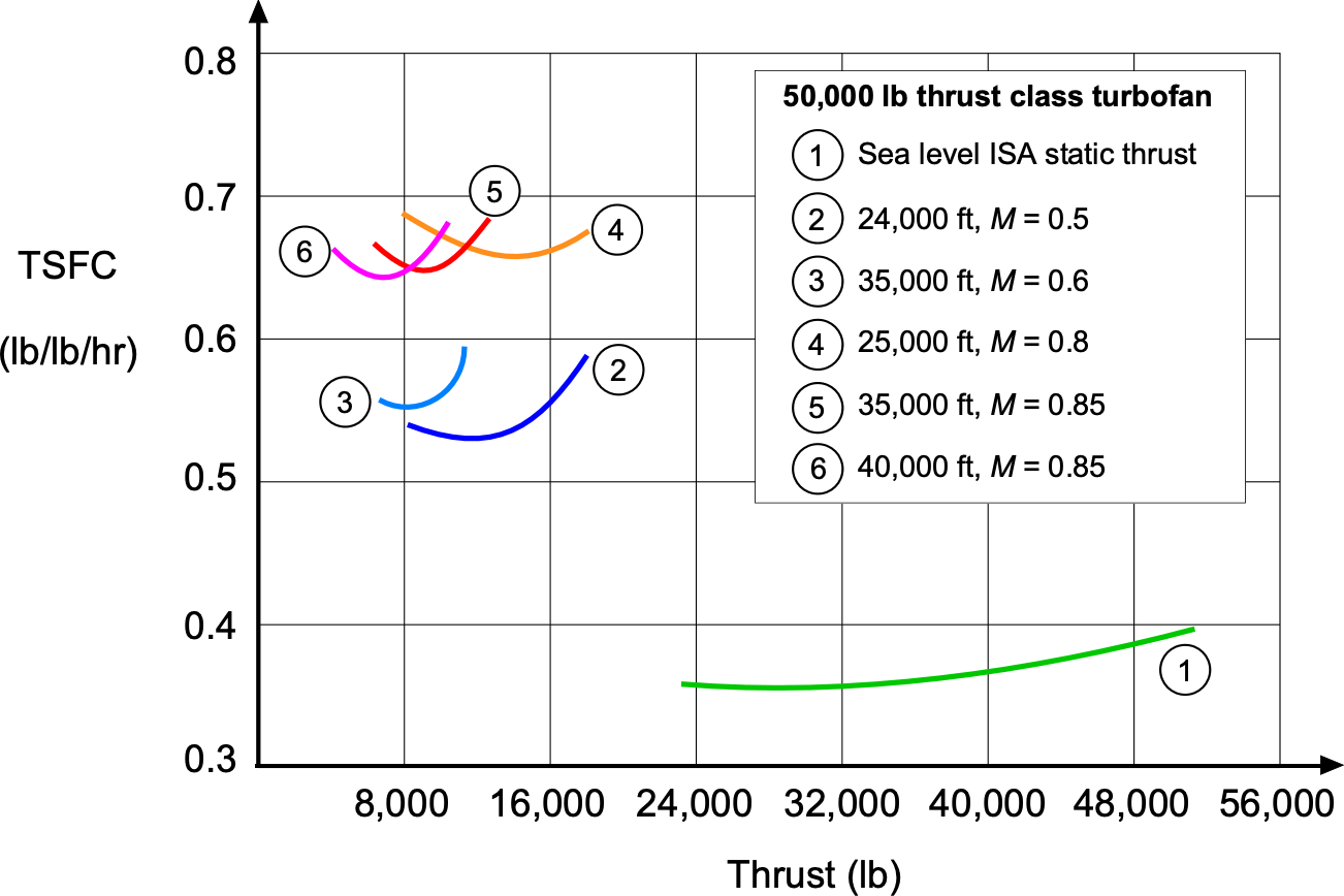
A complication in dealing with internal combustion engines (reciprocating or jet) is that BSFC or TSFC values are generally not constant and depend on the engine throttle setting. In the case of jet engines, the TSFC also depends on the altitude and flight Mach number at which it operates, as shown in the figure below for a modern turbofan (note that the TSFC scale exaggerates the differences). At any given flight condition, both thrust and specific fuel consumption (SFC) vary together as the throttle setting changes. When plotted on a graph of thrust versus SFC, the data form a curved line known as a thrust hook.
More detailed performance calculations always require carefully modeling the specific engine performance characteristics, which necessitates the use of engine charts or engine decks.[2] a data set that describes the engine’s performance across its full operating range. Aircraft designers use engine decks to model propulsion performance and fuel consumption throughout the flight envelope. Such detailed information about engine performance is typically available only to aircraft manufacturers planning to use the engine on their aircraft.
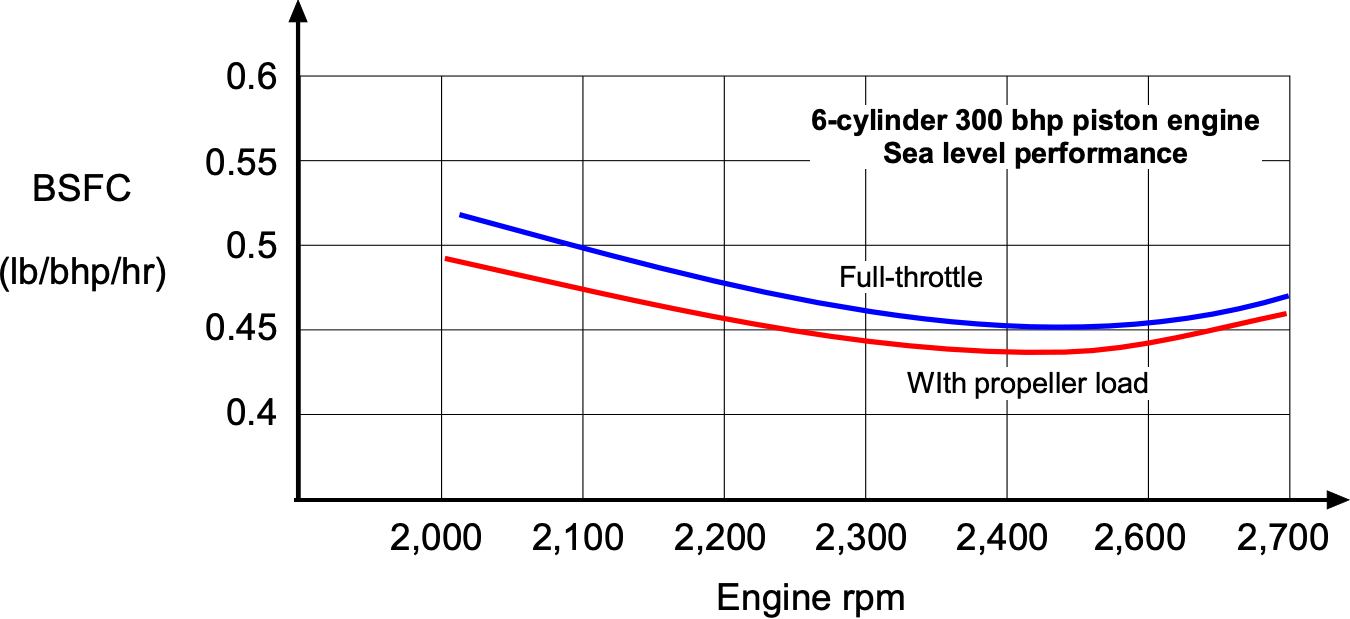
Piston engine performance (at least for normally aspirated engines) does not depend substantially on airspeed, but it will depend on density altitude, i.e., the altitude corresponding to the ambient pressure and temperature as measured in the ISA. All variants of these engines are typically designed to achieve their best (lowest) BSFC when operating at wide-open throttle and at or near their rated power, appropriate to the airplane they are selected to propel, as shown in the figure below. At lower throttle settings, the BSFC tends to increase slightly, meaning the engine becomes less efficient and burns more fuel per unit of power. For a normally aspirated piston engine, BSFC typically decreases (improves) at altitudes up to approximately 10,000 feet (~3,000 meters), then increases again at higher altitudes. With a supercharged engine, however, the BSFC stays relatively constant at all operational altitudes.
Because the BSFC or TSFC curves for aircraft engines are often relatively flat (constant) over the range of almost wide-open throttle settings used in flight, it is a reasonable assumption for an aircraft engine to assume that the BSFC or TSFC is constant. This latter assumption helps estimate net fuel burn during flight at different airspeeds, weights, and operating altitudes, at least in the first iteration, where detailed engine performance characteristics may not be available. However, BSFC or TSFC characteristics must be known (or estimated) to properly determine actual fuel burn.
Therefore, if the BSFC or the TSFC is known, then the corresponding fuel flow rate curves can be determined (estimated) because they are proportional to the power required for a propeller-driven airplane and the thrust for a jet-driven airplane. A generic fuel flow example is shown in the figure below. Notice that there is an airspeed on the fuel flow curve at which the minimum fuel flow is required for flight (point A) and also an airspeed at which the ratio of airspeed to fuel flow is a maximum (point B), both of which are significant in terms of flight operations.
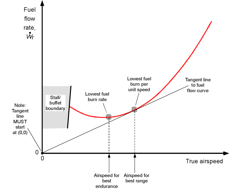
For a given quantity of fuel carried on the airplane, the airspeed to fly for minimum fuel flow (point A) corresponds to the flight conditions that achieve the longest flight time, i.e., the maximum flight endurance. The tangent of the straight line from (0,0) to the fuel flow curve (point B) corresponds to the condition that the airspeed ratio to fuel flow is at a maximum. Because distance (in still air or zero winds) is the product of airspeed and a given flight time, point A corresponds to the furthest still air distance covered for a given quantity of fuel, i.e., this will be the airspeed to fly to achieve the best range.
Fuel Flow Curves – Propeller Airplanes
The power required,  , for a propeller-driven airplane is assumed to be the brake power required (i.e., the brake power at the shaft,
  ), which will also reflect the effects of the propeller efficiency, i.e.,
(3) 
A constant-speed propeller will have a propulsive efficiency,  , that will be reasonably constant over the normal range of flight speeds. This assumption is reasonable for analyzing turboprop and high-performance piston-engine aircraft. The propulsive efficiency of a fixed-pitch propeller is not constant; it can vary significantly with airspeed. Therefore, the aircraft performance analysis requires consideration of the propeller charts to determine at actual flight conditions. Notice that in most cases, the density of the air has been referenced to ISA conditions, where
  , and the value of
  comes from the ISA equations.
If it is assumed that the engine BSFC is constant (this is a reasonable but not a general assumption), then the fuel flow (in appropriate units of time) will be
(4) 
where the BSFC is now denoted by . The fuel flow is, therefore,
(5) 
(6) 
for a constant weight and/or altitude, where
(7) 
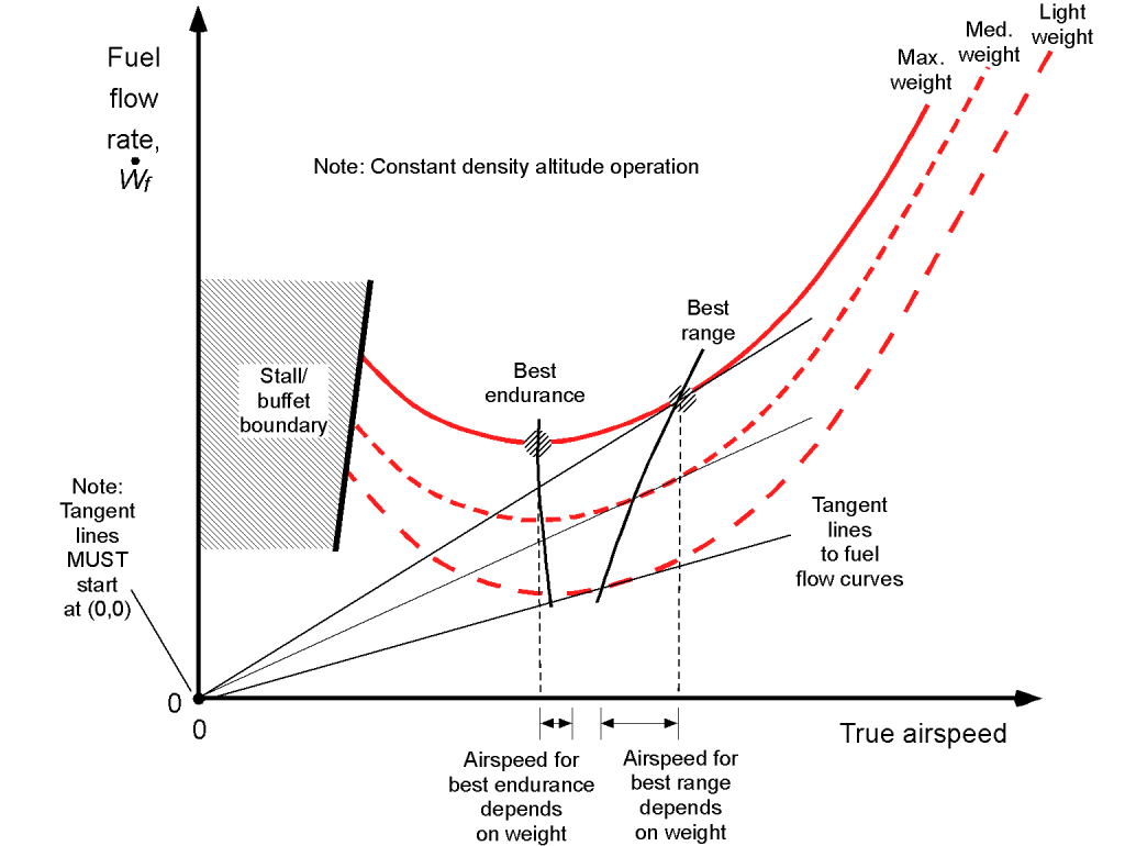
Remember the general “U” shaped characteristic of the power required for a propeller-driven airplane flight curve; these power curves are a function of airspeed and depend on the weight of the airplane and the equivalent density altitude at which it is flying. Therefore, the fuel flow curves will mimic the shapes of the power curves. For example, the effects of the airplane’s in-flight weight on its fuel flow characteristics are shown in the figure below. Notice that a higher flight weight increases the power and the corresponding fuel required. Additionally, the points for best endurance (lowest fuel flow) and best range (lowest fuel flow per unit speed or distance) are indicated; however, these speeds are not constant and depend on the flight weight.
The speed to fly for the lowest fuel burn (hence maximum flight endurance) can be determined by finding when  is a minimum. Differentiating the fuel flow result given by Eq. 6 with respect to
  gives
gives
(8) 
which is zero for a minimum, i.e.,
(9) 
and so the speed to fly for the best endurance will be
(10) 
confirming that  will depend on both weight and altitude. The corresponding lift coefficient is
(11) 
The best range is obtained when the ratio  is a minimum. In this case
(12) 
so that
(13) 
which is zero for a minimum, i.e.,
(14) 
(15) 
also confirming that  will depend on both weight and altitude, and where the corresponding lift coefficient is given by
(16) 
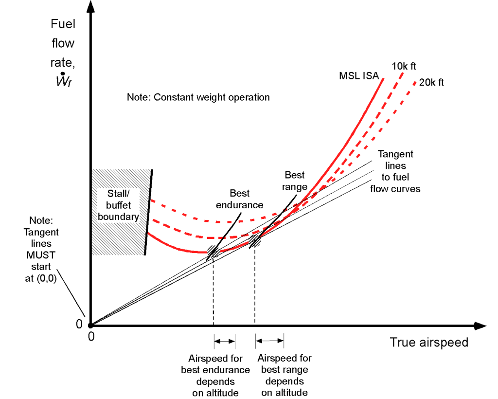
The effects of altitude on the fuel flow characteristics are shown in the figure below. Notice that at lower airspeeds, the effects of altitude increase the power required, resulting in a higher fuel flow. This outcome is because it can be deduced that at low airspeeds, the power required is dominated by the induced component (see Eq. 6). Again, the points for best endurance (lowest fuel flow) and best range (lowest fuel flow per unit speed or distance) are indicated; these speeds are not constant and depend on the weight and can be calculated using Eqs. 10 and 15, respectively.
Fuel Flow Curves – Jet Airplanes
As for propeller-driven airplanes, the fuel flow for a jet aircraft will be a function of airspeed, in-flight weight, and operating altitude. While the shapes of the fuel flow curves are different because they depend on thrust, they retain the qualitative U-shapes described by the thrust-required equation, i.e.,
(17) 
If it is assumed that the TSFC is constant (again, this is a reasonable assumption), then the fuel flow (in appropriate units of time) will be
(18) 
where the TSFC is now denoted by . The fuel flow is, therefore,
(19) 
which, in this case, is of the form
(20) 
for a constant weight and/or altitude, where
(21) 
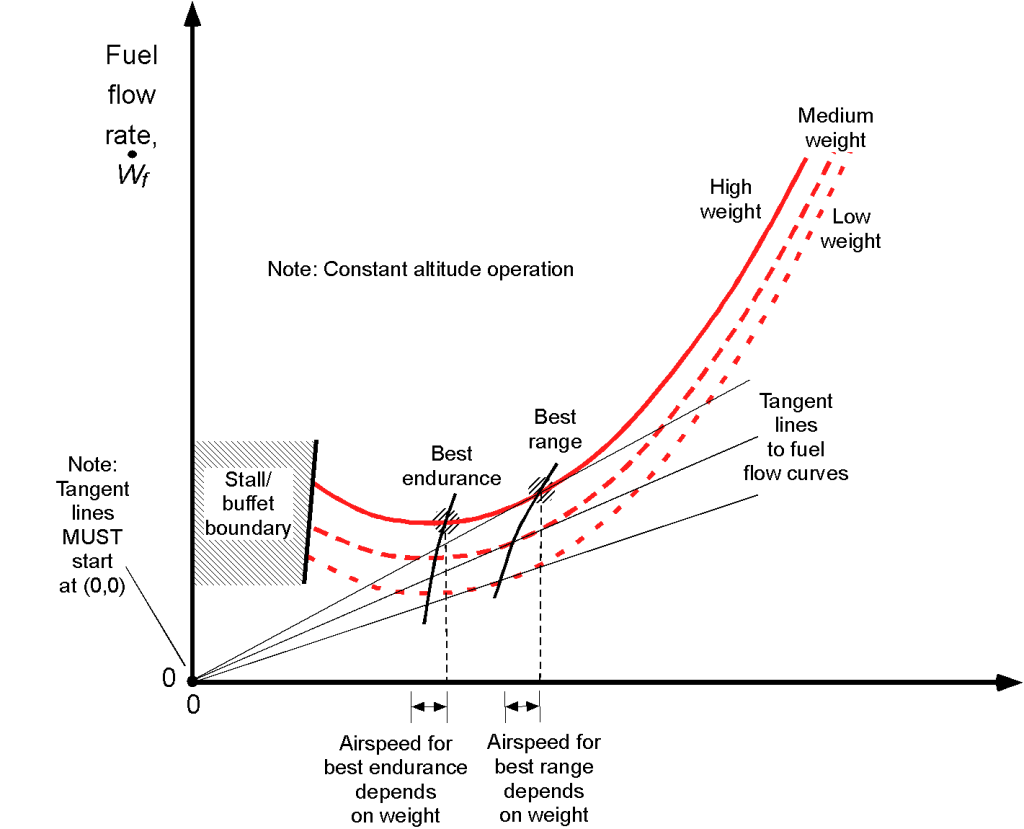
The effects of the jet airplane’s in-flight weight on the fuel flow characteristics are shown in the figure below. Notice again that a higher flight weight increases the power and fuel required. The points for best endurance (lowest fuel flow) and best range (lowest fuel flow per unit speed or distance) are indicated; these speeds depend on the airplane’s weight.
The speed to fly for the lowest fuel burn (hence maximum flight endurance) can be determined by finding when is a minimum. Differentiating the fuel flow result given by Eq. 20 with respect to gives
(22) 
which is zero for a minimum, i.e.,
(23) 
and so the speed to fly for the best endurance for a jet aircraft will be
(24) 
confirming that will depend on both the weight of the airplane and its operating altitude. The corresponding lift coefficient is
(25) 
As previously discussed, the best range is obtained when the ratio is a minimum. In this case, for a jet, then
(26) 
so that
(27) 
which is zero for a minimum, i.e.,
(28) 
(29) 
Additionally, it is confirmed that will depend on both weight and altitude for a jet. The corresponding lift coefficient is
(30) 
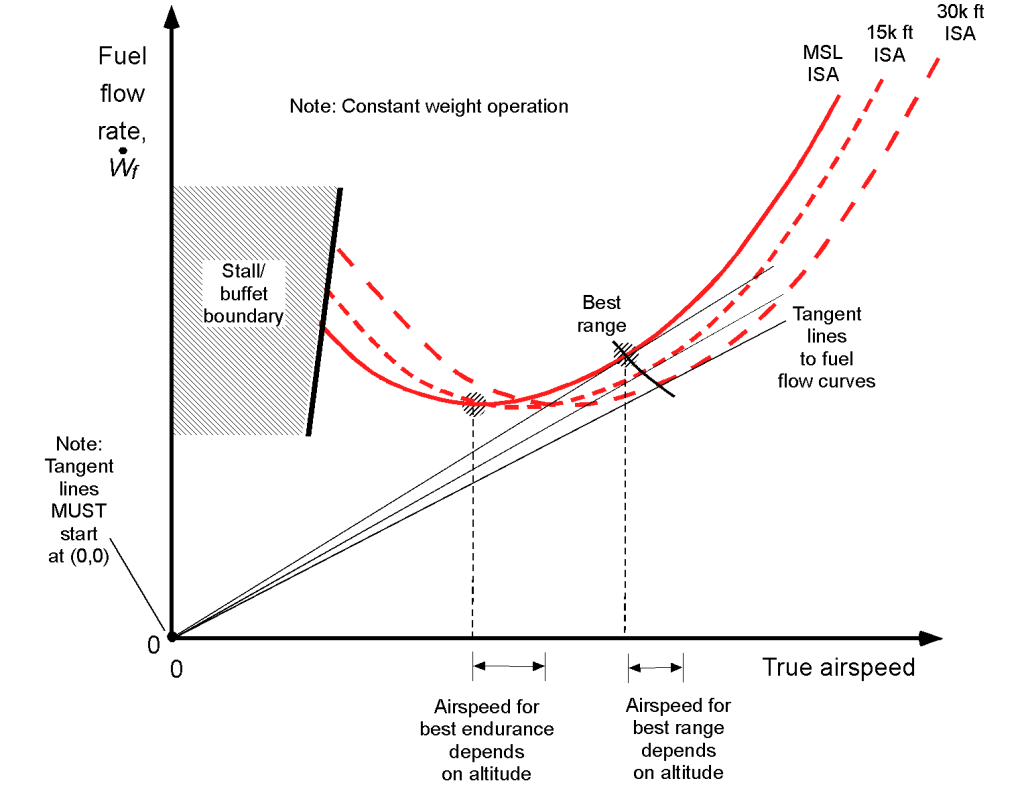
The effects of altitude on the fuel flow characteristics are shown in the figure below. Notice that at lower airspeeds, the effects of altitude increase the power required, resulting in a higher fuel flow. Again, the points for best endurance (lowest fuel flow) and best range (lowest fuel flow per unit speed or distance) are indicated; these speeds are not constant and depend on the weight and can be calculated using Eqs. 24 and 29, respectively.
Total Fuel Burn
Determining the aircraft’s total fuel burn over the intended flight or mission requires knowing the fuel flow as a function of aircraft weight, operating altitude, and true airspeed (or Mach number). While the fuel flow curves have previously been delineated for the separate effects of weight and altitude, the aircraft’s weight, altitude, and airspeed can vary continuously during flight. Additionally, the climb and descent phases of the flight must be considered. Therefore, the net fuel burn is calculated by summing the fuel burned for each flight segment. An estimated fuel burn will be used for flight planning, so sufficient fuel for the flight (plus reserve) can be loaded onto the aircraft.
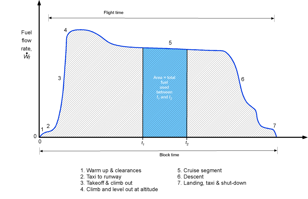
A representative fuel flow rate versus time is shown in the figure below for a typical civil flight, including takeoff, climb, cruise to a destination, and landing. By integration over time, the total fuel burned can be determined in units of weight, i.e., for the interval between  and
and  , then the weight of fuel burned is
(31) 
which is just the area under the fuel flow curve between  and
and  . The total fuel burn, therefore, is the total area under the fuel flow curve from takeoff to landing.
As a special case, if is assumed to be constant (which is reasonable over relatively short flight times in the cruise segment of flight), then the weight of fuel burned,  , would be
(32) 
In general, however, the total fuel burn for each flight segment must be obtained by integration.
If the initial weight of the airplane at  is
is  and the fuel available is , then when all of this fuel is burned, the new weight of the airplane at
  will be
  . Using a propeller-driven airplane as an example, the change in weight of the airplane with time will be
(33) 
so rearranging and integrating gives
(34) 
The minus sign indicates that the airplane’s weight  decreases with time, rectified by reversing the limits of integration. Therefore, the flight time corresponding to the fuel burned will be
(35) 
If is further assumed to be the total fuel available, then  , in this case, becomes the endurance
  , i.e.,
(36) 
which would use all the available fuel. Again, as a special case, if and are assumed to be constant, then the flight endurance for a given fuel weight would be
(37) 
Regarding range, the interest here is in the distance covered over the ground for a given quantity of fuel. Multiplying both sides of Eq. 33 by gives
(38) 
and then rearranging gives
(39) 
The distance covered in a given time, or the range  , is then
(40) 
which gives
(41) 
so that
(42) 
where  . The physical meaning of this integral is also related to the area under the fuel flow curve. Again, as a special case, if and are assumed to be constant, then the flight range for a given fuel weight would be
(43) 
Reserve fuel: Why is it needed?
The need for reserve fuel must always be considered when estimating flight range. For example, the flight crew may reach a final destination to find air traffic delays or bad weather preventing landings. The aircraft may also need to enter a holding pattern or divert to an alternative airport. For this reason, reserve fuel is always required. The FAA regulations (FARs) mandate that all aircraft carry extra reserve fuel. For VFR (Visual Flight Rules) conditions, the aircraft must carry 30 minutes of reserve fuel in addition to the estimated fuel required for the planned flight. For IFR (Instrument Flight Rules) conditions, the FAA requirement is to have 45 minutes of reserve fuel.
Breguet Equations
The preceding principles are formally embodied in the Breguet equations for airplane endurance and range, first developed by Louis Charles Breguet. These are some of the most famous equations used in aeronautical engineering. Understanding how they are derived is crucial, as is recognizing what information they can reveal about an airplane’s flight performance.
Breguet Endurance Equation – Propeller Airplanes
For flight endurance, it has been previously stated that the endurance is given by
(44) 
Assuming lift equals weight ( ) and
) and  , then in level flight the endurance is
(45) 
The lift required (which must equal the weight) is
(46) 
so solving for the airspeed gives
(47) 
Also, for the drag on the aircraft, then
(48) 
Substituting the previous results means that the endurance equation now becomes
(49) 
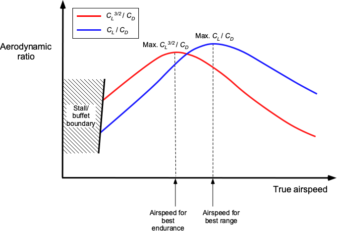
Notice that the ratio  appears in this latter equation, not the lift-to-drag ratio
  . While the numerical values are similar, the airspeeds at which the maximum values occur are distinctly different, as shown in the figure below.
Proceeding further by assuming that the value of is constant over the flight time, which might be reasonable for shorter flight times where the weight of the airplane does not change by much, as well as assuming that , and are constant (i.e., the airplane is flying at a constant altitude), then after integration of Eq. 49 the endurance will be
(50) 
which is known as the Breguet endurance equation for a propeller-driven airplane.
The latter equation estimates the flight endurance for a given total fuel weight. If no assumptions were made before the analytic integration, finding the required fuel and endurance would usually have to be performed entirely by numerical integration.
Therefore, from the Breguet endurance equation, it becomes clear that to maximize flight endurance, the airplane must be flown in such a way that:
- The propeller is operated at (or near) its best propulsive efficiency; this is typical of a constant speed (variable pitch) propeller.
- The engine is operated at (or near) the power setting to achieve its best BSFC, although this may not be possible at lower power settings, which are likely to be altitude-dependent.
- The airplane carries the largest quantity of fuel. However, fuel quantity may be limited by factors other than tankage volume, such as the need to carry a specific payload, which must be traded off against the fuel load.
- The airplane flies at (or close to) the best aerodynamic ratio of .
Breguet Range Equation – Propeller Airplanes
Now, consider the flight range of the propeller-driven airplane. As was previously established, the range is given by
(51)
After the substitution of the relationships used previously for endurance, then
(52) 
Again, for steady level flight, , so
(53) 
where in this case the lift-to-drag ratio is involved.
As performed before with the endurance integral, if , and are assumed to be constant then
(54) 
which, after integration, leads to an estimate for the range as
(55) 
which is usually known as the Breguet range equation. Again, if the actual values of , , and  corresponding to a given flight condition were to be used, then the integral would need to be evaluated numerically.
Statute Miles or Nautical Miles?
Nautical miles are used to measure distances in the aeronautical and aviation world. A nautical mile is 1/60th of a degree or one minute of latitude and is 6,076 ft or 1,852 m long. Speed is typically measured in nautical miles per hour (nmi/h) or knots (kts), and airplane airspeed indicators are calibrated in knots. The familiar land mile is a statute mile, measuring 5,280 ft, based on a Roman measure of 1,000 paces. The statute mile was standardized as exactly 1,609.344 meters by an international agreement in 1959. A nautical mile is abbreviated to “M” or “NM,” but more usually, “nm” is used. The statute mile was previously abbreviated to “m” but is now written as “mi'” to avoid confusion with the SI unit meter (or metre).
Therefore, based on the preceding, it is clear that to maximize the flight range, the airplane must be flown in such a way that:
- As previously discussed, the propeller is operated at (or near) its best propulsive efficiency.
- The engine is operated at (or near) the power setting to achieve its best BSFC, again with the caveats previously discussed.
- The airplane carries the largest quantity of fuel.
- The airplane flies at or near the best lift-to-drag ratio .
In summary, when thinking about the design of a propeller-driven airplane, achieving the best flight endurance and/or range is about four things:
- Carrying as much fuel as possible.
- Achieving a high aerodynamic efficiency from the airframe, i.e., designing the airplane to minimize drag as much as possible.
- Striving for high engine efficiency, i.e., obtaining the lowest possible value of BSFC from the engines.
- Obtaining high propulsive efficiency, i.e., designing the propeller in this case for optimal overall aerodynamic efficiency, will inevitably require a variable-pitch (i.e., constant-speed) propeller.
Check Your Understanding #1 – Finding the range of a propeller-driven airplane
A small propeller-driven aircraft is flying along at an estimated in-flight weight of 2,100 lb and an airspeed of 120 knots at 2,000 ft, where the air density is 0.00216 slugs/ft . The airplane only has 8 gallons of usable fuel (excluding reserves), and the pilot must fly 120 nautical miles to the home airport. Is there enough fuel to do this? Assume no winds. The engineering characteristics of the aircraft are wing span,
  = 36 ft, wing area,
  = 174 ft
 , non-lifting drag coefficient,
  = 0.02, propeller efficiency, = 0.85, Oswald’s efficiency factor,
  = 0.81, and BSFC, = 0.45 lb bhp hr.
Show solution/hide solution.
There are only 8 gallons of AVGAS fuel, and AVGAS weighs 6.0 lb per gallon, so = 48 lb of fuel. An airspeed of 120 kts is equivalent to 120  1.688 = 202.54 ft/s = . The initial operating lift coefficient of the wing,
  , is
, is
![\[ C_L = \frac{2W}{\varrho \, V^2 S} = \frac{2 \times 2,100}{0.00216 \times 202.54^2 \times 174.0} = 0.272 \]](https://eaglepubs.erau.edu/app/uploads/quicklatex/quicklatex.com-39bdb6620bdcd5aa40e43ab5971e7997_l3.svg "Rendered by QuickLaTeX.com")
To find the induced drag coefficient, the aspect ratio of the wing,  , is needed, i.e.,
![\[ A\!R = \frac{b^2}{S} = \frac{(36.0)^2}{174.0} = 7.45 \]](https://eaglepubs.erau.edu/app/uploads/quicklatex/quicklatex.com-bc2078e4cf5d4df8544aed081cbd1414_l3.svg "Rendered by QuickLaTeX.com")
The induced drag coefficient  will be
![\[ C_{D_{i}} = \frac{{C_L}^2}{\pi \, A\!R \, e} = \frac{0.272^2}{\pi \times 7.45 \times 0.81} = 0.0039 \]](https://eaglepubs.erau.edu/app/uploads/quicklatex/quicklatex.com-0fb4ec2659681d3a45bddca61765d817_l3.svg "Rendered by QuickLaTeX.com")
Therefore, the total drag coefficient,  , is
, is
![\[ C_D = C_{D_0} + C_{D_i} = C_{D_0} + \frac{{C_L}^2}{\pi \, A\!R \, e} = 0.02 + 0.0039 = 0.0239 \]](https://eaglepubs.erau.edu/app/uploads/quicklatex/quicklatex.com-3492526d0cbf9ad4c24f28f5d54c3382_l3.svg "Rendered by QuickLaTeX.com")
and the lift-to-drag ratio of the aircraft at the given conditions of flight is
![\[ \frac{L}{D} = \frac{C_L}{C_D} = \frac{0.272}{0.0239} = 11.38 \]](https://eaglepubs.erau.edu/app/uploads/quicklatex/quicklatex.com-b4b0f99c5d234a05896f1a1b4b1af482_l3.svg "Rendered by QuickLaTeX.com")
The Breguet range equation for a propeller-driven airplane is
![\[ R = \frac{\eta_p}{c_b} \left( \frac{C_L}{C_D}\right) \ln \left( \frac{W_0}{W_0-W_f}\right) \]](https://eaglepubs.erau.edu/app/uploads/quicklatex/quicklatex.com-ae814d8940972fcf5fb1c219647e60c2_l3.svg "Rendered by QuickLaTeX.com")
IMPORTANT: Notice that the value of the brake-specific fuel consumption or BSFC in this problem is given in units of lb bhp hr, which must be converted to base units before using it in the Breguet equation. One brake horsepower (bhp) is equivalent to 550 ft-lb s, and there are 3,600 seconds in an hour, i.e., by dividing the given value by 550 x 3,600.
Therefore, inserting the known values gives the potential approximate range of the aircraft as
![\[ R = \frac{0.81 \times 550 \times 3,600}{0.45} \left( 11.38 \right) \ln \left( \frac{2,100}{2,100 -48}\right) = 984,118~\mbox{ft} \]](https://eaglepubs.erau.edu/app/uploads/quicklatex/quicklatex.com-cc8fd7ac16f0b49b9ad3706d340bacdc_l3.svg "Rendered by QuickLaTeX.com")
which is approximately 162 nautical miles. In conclusion, the aircraft has sufficient fuel to reach the home airport with a margin, allowing the pilot to relax and enjoy the remainder of the flight.
Breguet Endurance Equation – Jet Airplanes
In evaluating jet airplane performance, the thrust required by the engine is the primary factor affecting fuel burn. However, the estimation of endurance and range proceeds along a similar path to that previously used for the propeller-driven airplane.
For a jet engine, the thrust-specific fuel consumption (TSFC) is defined as
(56) 
in units of lb lb hr. Therefore, the fuel flow rate is
(57) 
where  is the required thrust from the engine. Therefore, to determine the fuel flow rate, the thrust required from the engine must be calculated; in level flight, this equals the airplane’s drag.
As fuel is burned, the weight of the airplane changes proportionally, so the change in weight of the airplane is
(58) 
The airplane’s weight is  at time
  and
and  at time
  , where is the initial weight minus the fuel burned, i.e., . Therefore,
(59) 
which gives the time of flight, , to burn the fuel weight, . Now, if is the total fuel available then is equal to the endurance so
(60) 
For level flight then  and and after substitution then
(61) 
It will be noted immediately that this is a different result from the propeller-driven airplane because, in this case, the endurance depends on and not for the propeller airplane.
By assuming that and are constant, the foregoing endurance equation integrates out to be
(62) 
which is referred to as the Breguet endurance equation for a jet airplane.
Therefore, to maximize the flight endurance of a jet airplane, it must be flown in such a way that:
- The engine(s) is/are operated at (or near) the power setting to achieve their best TSFC. For most jet engines, this condition inevitably occurs at higher altitudes, which is by design.
- The airplane carries the largest quantity of fuel, although this may be limited by weight rather than available tankage.
- The airplane flies at or near the best lift-to-drag ratio .
Breguet Range Equation – Jet Airplanes
As before, the differential equation to account for the change in the weight of the airplane as fuel is burned is
(63)
or by rearrangement
(64) 
The distance flown is the product of airspeed and time, so multiplying both sides of the preceding equation by gives
(65) 
noticing that the term on the left-hand side is simply distance, denoted by  . The airplane’s weight is at time and at time , where is the initial weight minus the fuel burned, i.e., . Integrating Eq. 65 gives
(66) 
For level flight, then and , and after the substitution, the distance traveled on a given weight of fuel is
(67) 
which would be the maximum range if the value of was all the useful fuel. Also
(68) 
so that after substitution, the range of the airplane becomes
(69) 
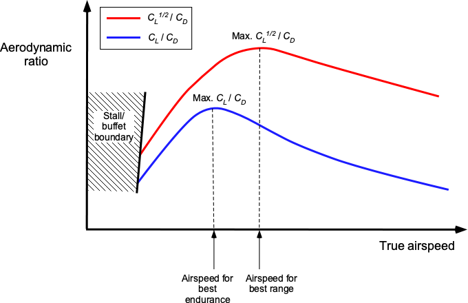
which again yields a different result to the propeller-driven airplane, as it depends on the aerodynamic ratio  rather than
  , as shown in the figure below. The airspeed for the best value of , and so the best range, is generally significantly higher than that for best endurance.
By assuming that , , and are constant, the foregoing endurance equation integrates out to be
(70) 
which is referred to as the Breguet range equation for a jet airplane.
Therefore, to maximize the flight range of a jet airplane, it must be flown in such a way that:
- The engine operates at (or near) the thrust (throttle) setting to achieve its best TSFC.
- The airplane carries the largest quantity of fuel.
- The airplane flies at or near the best value of the aerodynamic ratio .
Check Your Understanding #2 – Finding the range of a jet aircraft
A small, single-engine, jet-powered aircraft has an initial in-flight weight, , of 5,000 lb and carries 1,000 lb of usable fuel. The aircraft is at an altitude of 25,000 ft ISA. Its drag polar can be expressed as  . It has a wing area of 180 ft2. The TSFC of the engine is = 1.0 lb/lb/hr. What is the best range of the aircraft in these conditions, and at what airspeed should the pilot fly to reach this range?
Show solution/hide solution.
For a jet aircraft, the conditions for maximum range are achieved when the aerodynamic ratio  is maximized. If the drag polar is
![\[ C_D = C_{D_{0}} + k \, C_L^ {\,2} = 0.018 + 0.095 \, C_L^ {\,2} \]](https://eaglepubs.erau.edu/app/uploads/quicklatex/quicklatex.com-d153077d99579805444fe8ed826a23fa_l3.svg "Rendered by QuickLaTeX.com")
then
![\[ \frac{C_D}{C_L^{1/2}} = \frac{ C_{D_{0}} + k \, C_L^ {\,2}}{C_L^{1/2}} = \frac{C_{D_{0}}}{C_L^{1/2}} + k C_L^{\, 3/2} \]](https://eaglepubs.erau.edu/app/uploads/quicklatex/quicklatex.com-ba02c47dd1b178ff1fd2769a3a7361e1_l3.svg "Rendered by QuickLaTeX.com")
To find a maximum (or minimum), the preceding expression is differentiated with respect to and then set to zero, i.e.,
![\[ \frac{ d (C_D/C_L^{1/2})}{d C_L} = -\frac{1}{2} \left( \frac{C_{D_{0}}}{C_L^{1/2}} \right) + \frac{3}{2} k C_L^{1/2} = 0 \]](https://eaglepubs.erau.edu/app/uploads/quicklatex/quicklatex.com-cfb5444fb453f3a27075f2e5bee57a50_l3.svg "Rendered by QuickLaTeX.com")
Therefore, the needed lift coefficient for this best range condition is
![\[ C_L = \sqrt{ \frac{C_{D_{0}}}{K} } = \sqrt{ \frac{0.018}{0.095} } = 0.251 = C_{L_{\rm br}} \]](https://eaglepubs.erau.edu/app/uploads/quicklatex/quicklatex.com-714fc760441ae741ba88428c03b55850_l3.svg "Rendered by QuickLaTeX.com")
The corresponding drag coefficient will be
![\[ C_D = 0.018 + 0.095 \, C_L^ {\,2} = 0.018 + 0.095 \times 0.251^2 = 0.024 \]](https://eaglepubs.erau.edu/app/uploads/quicklatex/quicklatex.com-ee813dc997fb26d1456ce2bd1ede2b7a_l3.svg "Rendered by QuickLaTeX.com")
Therefore,
![\[ \left( \frac{ C_L^{1/2}}{ C_D} \right)_{\rm br} = \frac{ 0.251^{1/2}}{0.024} = 20.875 \]](https://eaglepubs.erau.edu/app/uploads/quicklatex/quicklatex.com-072ae34bd7534b06011ebc4fc8954dfe_l3.svg "Rendered by QuickLaTeX.com")
The Breguet range equation for a jet aircraft is
![\[ R = \frac{2}{c_t} \sqrt{ \frac{2}{\varrho_0 \, \sigma S}} \left(\frac{C_L^{1/2}}{C_D} \right)_{\rm br} \left( W_0^{1/2} - W_1^{1/2} \right) \]](https://eaglepubs.erau.edu/app/uploads/quicklatex/quicklatex.com-bcf169abfaf55a283ffbe814f3138d8a_l3.svg "Rendered by QuickLaTeX.com")
The initial weight is = 5,000 lb, and the final weight, , is the initial weight, less the fuel weight burned, so = 4,000 lb. At an altitude of 25,000 ft ISA conditions,  =
=  = 0.001066 slug/ft3. It is essential to be cautious here and note that is expressed in units per hour, so a factor of 3,600 is required to convert to units per second. Inserting all the values gives
![\[ R = \frac{2\times 3,600}{1.0} \sqrt{ \frac{2}{0.001066 \times 180.0}} \left( 20.875\right) \left( 5,000^{1/2} - 4,000^{1/2} \right) \]](https://eaglepubs.erau.edu/app/uploads/quicklatex/quicklatex.com-3f685a9f13eb6c01889e950bc96fd6d4_l3.svg "Rendered by QuickLaTeX.com")
which gives = 3,622,400 ft = 596 nautical miles. The airspeed for the best range is obtained using
![\[ V_{\rm br} = \sqrt{ \frac{2 W}{\varrho_{\infty} \, S \, C_{L_{\rm br}}}} = \sqrt{ \frac{2 \times 5,000}{0.001066 \times 180.0 \times 0.251 }} = 455.7~\mbox{ft/s} \]](https://eaglepubs.erau.edu/app/uploads/quicklatex/quicklatex.com-32dd5343fbaa201a4ae1396d6cbccabf_l3.svg "Rendered by QuickLaTeX.com")
which is a true airspeed of 270 knots.
Best Airspeed for Maximum Range in a Wind
A common misconception is how wind affects the optimal range of an airplane. The key to resolving this issue is understanding the difference between the airplane’s speed through the air and its speed over the ground. It is essential to appreciate that the aerodynamics of an airplane are unaffected by winds. However, the wind most certainly affects the airplane’s speed over the ground. The effect of wind on the optimal speed to fly and the resulting fuel burn can be significant, especially on long-haul flights, where fuel consumption is a major component of the overall operational cost. The consequences depend on whether the aircraft is flying into a headwind or benefiting from a tailwind.
As previously discussed, the aircraft’s range in still air is determined by the Breguet range equation
(71) 
where is the range, is the true airspeed (TAS), is the specific fuel consumption,  is the lift-to-drag ratio, and
  and
and  are the initial and final airplane weights between two points in time, i.e., where is the weight of fuel burned during the time segment. For maximum range on a given weight of fuel, , the aircraft should fly at the airspeed that maximizes , denoted as , which depends on the airplane’s in-flight weight, cruising flight altitude, as well as its aerodynamics.
With a wind, the effective range of the airplane now depends on its ground speed,  . In this case, then its range is
(72) 
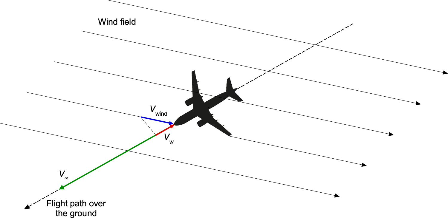
The ground speed is given by
(73) 
where  is the wind speed component in the direction of the flight path over the ground, which is positive for a direct tailwind, and negative for a direct headwind. In other wind directions, the component of the wind relative to the aircraft’s flight over the ground is what matters, as shown in the figure below.
The fuel flow rate is
(74) 
Differentiating with respect to true airspeed gives
(75) 
So that solving for the best in wind gives
(76) 
where  is the adjusted or “optimum” true airspeed for the best range with the wind, is the best range speed in still air, and is the wind speed.
Therefore, in a direct headwind ( ), the aircraft should be flown at a higher true airspeed to compensate for the reduced ground speed. In a direct tailwind (
 ), the airplane should be flown at a lower airspeed to take advantage of the additional ground speed provided by the wind. The correction factor
(77) 
gives the new airspeed to fly. This correction factor is necessary because the fuel flow per unit distance depends on ground speed, leading to an airspeed correction proportional to the cube root of the wind speed. Flying at the same best-range airspeed in a headwind reduces range because the airplane spends more time in the air, burning more fuel; therefore, it is best to fly a little faster. Flying at the same best-range airspeed with a tailwind wastes energy because the airplane could reach its destination faster, but slow down and still reach the destination much more efficiently in the same flight time.
For example, in still air, assume that the best range airspeed of a jetliner is = 450 kts. With a 50-knot direct headwind, then
(78) 
and the fuel burn per unit distance over the ground will increase by approximately 12.5%. With a 50-knot direct tailwind, then
(79) 
which results in a reduction in fuel burn of approximately 10%. These corrections can translate to thousands of pounds or kilograms of extra fuel burned or saved on long-haul flights. To this end, airlines actively optimize flight paths to avoid headwinds and capitalize on tailwinds, thereby conserving fuel.
Check Your Understanding #3 – Wind effects on the airspeed for the maximum range of a propeller-driven airplane
How does wind affect the optimal airspeed for maximum range in a propeller-driven airplane, and what is the mathematical correction for the best range speed in the presence of a wind?
Show solution/hide solution.
For a propeller-driven airplane, its range is given by the Breguet range equation for power-based fuel consumption, i.e,
![\[ R = \frac{\eta_p}{c_b} \frac{V_{\infty} (L/D)}{g} \ln \left(\frac{W_0}{W_1}\right) \]](https://eaglepubs.erau.edu/app/uploads/quicklatex/quicklatex.com-f6c6709b3708dd98c644a2e626d34c6d_l3.svg "Rendered by QuickLaTeX.com")
where is the range, is the propeller efficiency, is the brake-specific fuel consumption (i.e., = BSFC = fuel burned per unit power), is the true airspeed (TAS), is the airplane’s lift-to-drag ratio, and and  are the initial and final weights of the airplane, respectively.
For maximum range, the airplane should fly at the airspeed that minimizes power per unit airspeed, which occurs near the speed at minimum power required, i.e.,
![\[ V_{\rm br} = \text{speed at minimum power per unit airspeed} \]](https://eaglepubs.erau.edu/app/uploads/quicklatex/quicklatex.com-2495eda7650baacb06bf2c04ca74c989_l3.svg "Rendered by QuickLaTeX.com")
With a wind , the aircraft’s groundspeed is affected, i.e.,
![\[ V_{\rm gs} = V_{\infty} \pm V_{w} \]](https://eaglepubs.erau.edu/app/uploads/quicklatex/quicklatex.com-83dc5e22370dff1f40759bbff396f043_l3.svg "Rendered by QuickLaTeX.com")
Because the range of the airplane depends on its ground speed, fuel efficiency must be optimized with respect to . For a propeller aircraft, fuel flow is proportional to the power required, which is given by
![\[ P_{\text{req}} = D \times V_{\infty} \]](https://eaglepubs.erau.edu/app/uploads/quicklatex/quicklatex.com-0e6f9ff255e7985c8410eed63bb369c1_l3.svg "Rendered by QuickLaTeX.com")
where  is the drag on the airplane. Because we are maximizing the distance traveled over the ground per unit of fuel, then
![\[ \frac{\text{Fuel Flow Rate}}{V_{\rm gs}} = \frac{P_{\text{req}}}{V_{\rm gs}} = \frac{D V_{\infty}}{V_{\infty}} \pm V_{w} \]](https://eaglepubs.erau.edu/app/uploads/quicklatex/quicklatex.com-cef84278100a8cda77fb65d15b75dac1_l3.svg "Rendered by QuickLaTeX.com")
Differentiating with respect to and setting to zero gives
![\[ \frac{d}{dV_{\infty}} \left(\frac{V_{\infty}}{V_{\infty} \pm V_{w}} \right) = 0 \]](https://eaglepubs.erau.edu/app/uploads/quicklatex/quicklatex.com-83e972da58529668f49e8dfded6853ea_l3.svg "Rendered by QuickLaTeX.com")
Solving for gives the airspeed correction as
![\[ V_{\text{br,o}} = V_{\rm br} \times \left( 1 \pm \frac{V_{w}}{V_{\rm br}} \right)^{1/2} \]](https://eaglepubs.erau.edu/app/uploads/quicklatex/quicklatex.com-3d1200d3cb68d6f8dc2494eea571a35d_l3.svg "Rendered by QuickLaTeX.com")
Compared to a jet airplane, the correction in this case follows a square-root dependency, meaning that a propeller aircraft must increase speed more in headwinds and reduce speed more in tailwinds to optimize fuel efficiency. The outcome is that the impact of wind is greater for propeller-driven airplanes than for jet-propelled airplanes, primarily because of their lower cruise speeds, which make wind-speed corrections for optimal performance more critical in flight planning.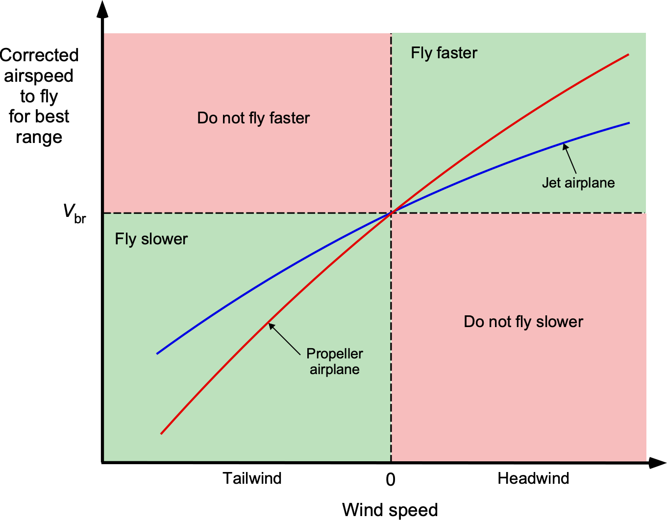
Payload-Range & Endurance Charts
The range that an airplane can fly on a given quantity of fuel depends on its weight and operating altitude. The weight of the aircraft is the sum of its empty weight plus the useful load, i.e., the weight of the payload and fuel. It takes fuel to carry the payload (i.e., passengers and/or cargo, which is what pays the bills), but fuel is not part of the payload. For most aircraft, there is a trade-off between payload and fuel load above a specific flight range, so the payload must be limited in exchange for increased fuel weight.
Airliners
The figure below illustrates a typical payload-range diagram for a commercial airliner. Airliners are point designs because they spend most of their flight time cruising at a constant airspeed (Mach number) and high altitudes. The typical shape of the payload-range diagram is such that the aircraft can carry a maximum payload only within a specified range, i.e., the gray area bounded by the horizontal line between points A and B. When an aircraft operates at maximum payload, the fuel tanks are generally not filled to their full capacity.
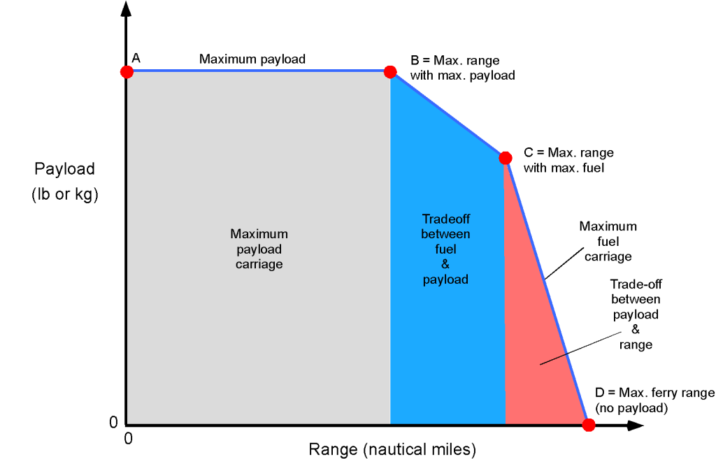
It can be seen from the diagram that longer flight ranges can be flown by reducing payload (i.e., limiting the number of passengers and cargo) in exchange for fuel, i.e., the blue area with the boundary marked between points B and C. Point C would be the maximum range with maximum fuel, i.e., the maximum fuel weight allowed for takeoff. However, for an airline, it would not make economic sense to operate in this region because it requires a significant reduction in payload to achieve a modest increase in range; in this case, using another airplane type or model might be a better option.
Along the boundary from C to D, the payload must be significantly reduced to achieve the required range; again, this would not be an economically viable operating condition. Point D would, for example, correspond to a ferry flight or to a situation in which a technical issue precludes carrying passengers, in which the aircraft is flown over an extended distance with maximum fuel but without any payload.
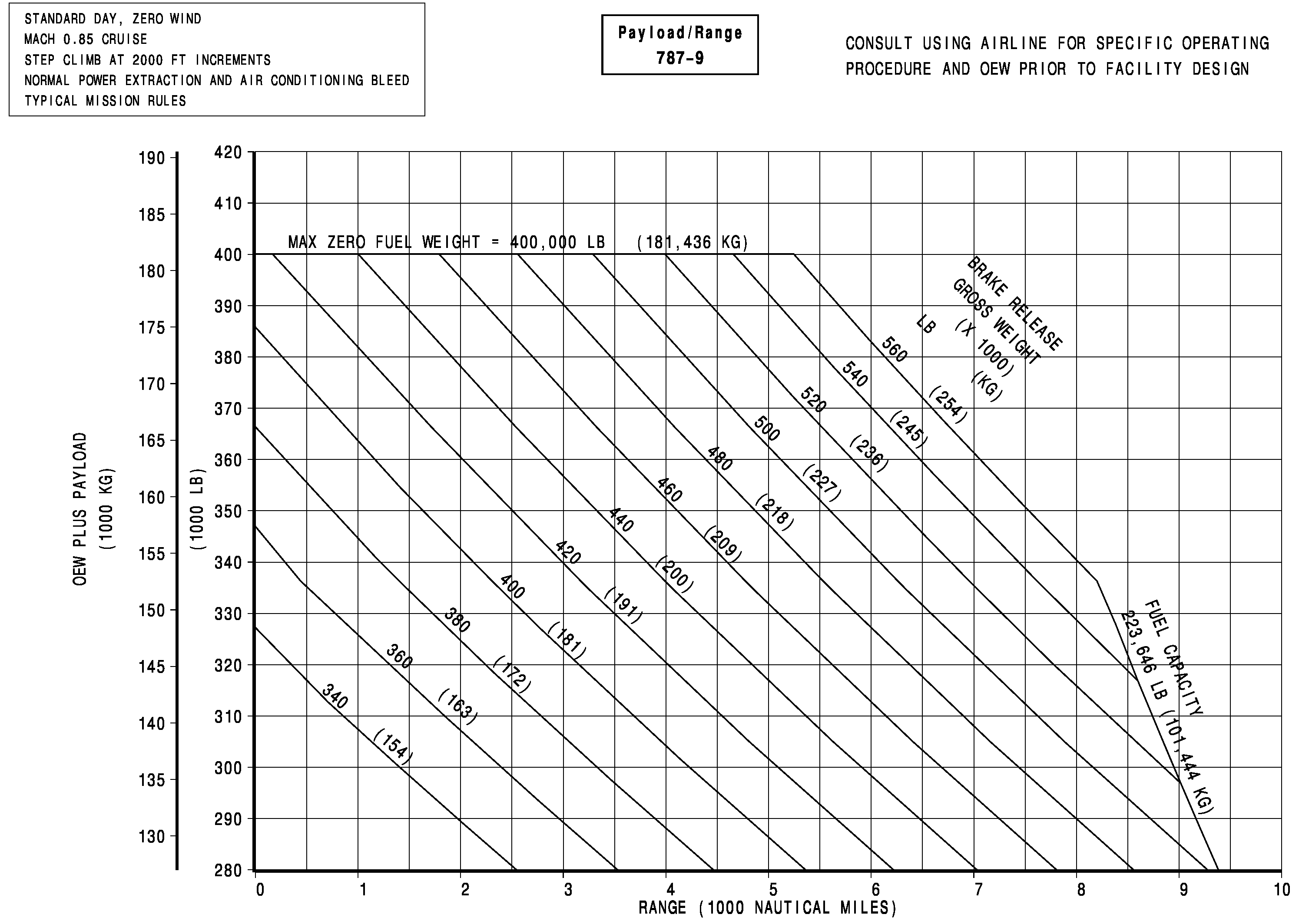
As an example, the payload-range chart for the Boeing B-787 Dreamliner is shown in the figure below. Notice that with a maximum payload of passengers and cargo, the aircraft has a range of over 5,000 nautical miles at a cruise Mach number of 0.85. To achieve greater ranges, the payload must be traded off to allow more fuel to be carried. With maximum fuel but a substantially reduced payload, the aircraft can achieve a range of over 8,000 nautical miles. However, as mentioned previously, this is unlikely to be an economically viable operating condition for an airline. Nevertheless, some airlines may opt for ultra-long-range flights with reduced passenger loads but introduce higher ticket prices, for example, by operating the entire aircraft in an all-business-class configuration.
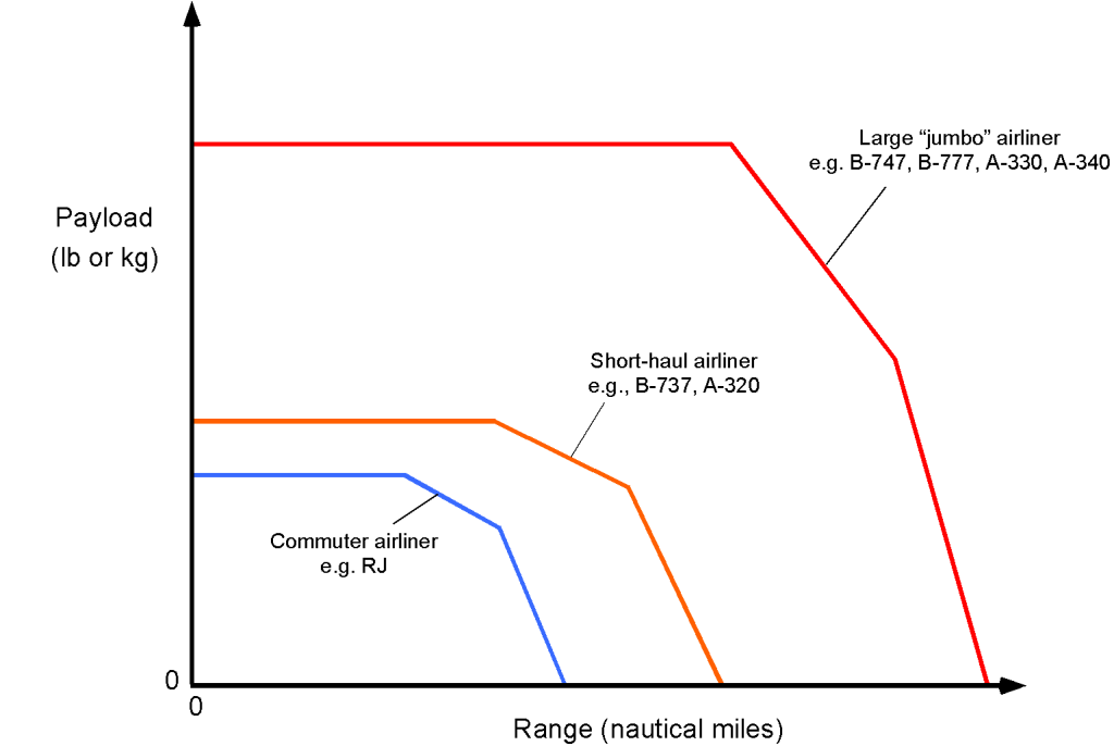
Of course, the payload-range chart will vary for each aircraft make and model. The payload and range of commercial airliners are carefully tailored to match specific route requirements, ultimately maximizing profit. Different models of the same airliner will have different range and payload capabilities, e.g., the B-737 and A320 series. More generally, however, there is not a “one-size fits all” solution, and airliners are designed for either commuter flights of less than 500 nautical miles, short-haul flights of between 1,000 and 2,000 miles, and long-haul flights for transcontinental and transoceanic distances of 4,000 to 5,000 miles, as shown in the payload-range chart below. For example, it would not make sense to operate a B-787 on short-haul segments when carrying only 100 passengers, and an RJ, with its more limited range, would require too many stops to be used for direct transcontinental flights.
Accessing payload-range and other performance characteristics
For access to airliner payload-range diagrams and other performance data, manufacturers provide “Airplane Characteristics for Airport Planning” documents. These include payload-range trade-offs, runway performance, airplane dimensions, and weight limitations. You can find these resources on the websites maintained by Boeing and Airbus, as well as on Embraer and Bombardier’s operator portals. These documents are essential for engineers, airport planners, and operators analyzing aircraft performance and airport compatibility.
Other Types of Aircraft
Of course, there are many other types of aircraft besides airliners, including general aviation (GA) aircraft and drones, for which payload, range, and endurance are also important. Therefore, pilots need to know, for example, the fuel required for a given range or the flight conditions that maximize range for flight planning. These aircraft types have relatively low payloads compared to their gross weight, so the payload-range tradeoff is not as severe as for an airliner. However, the aircraft’s range is still affected by altitude and engine power settings.
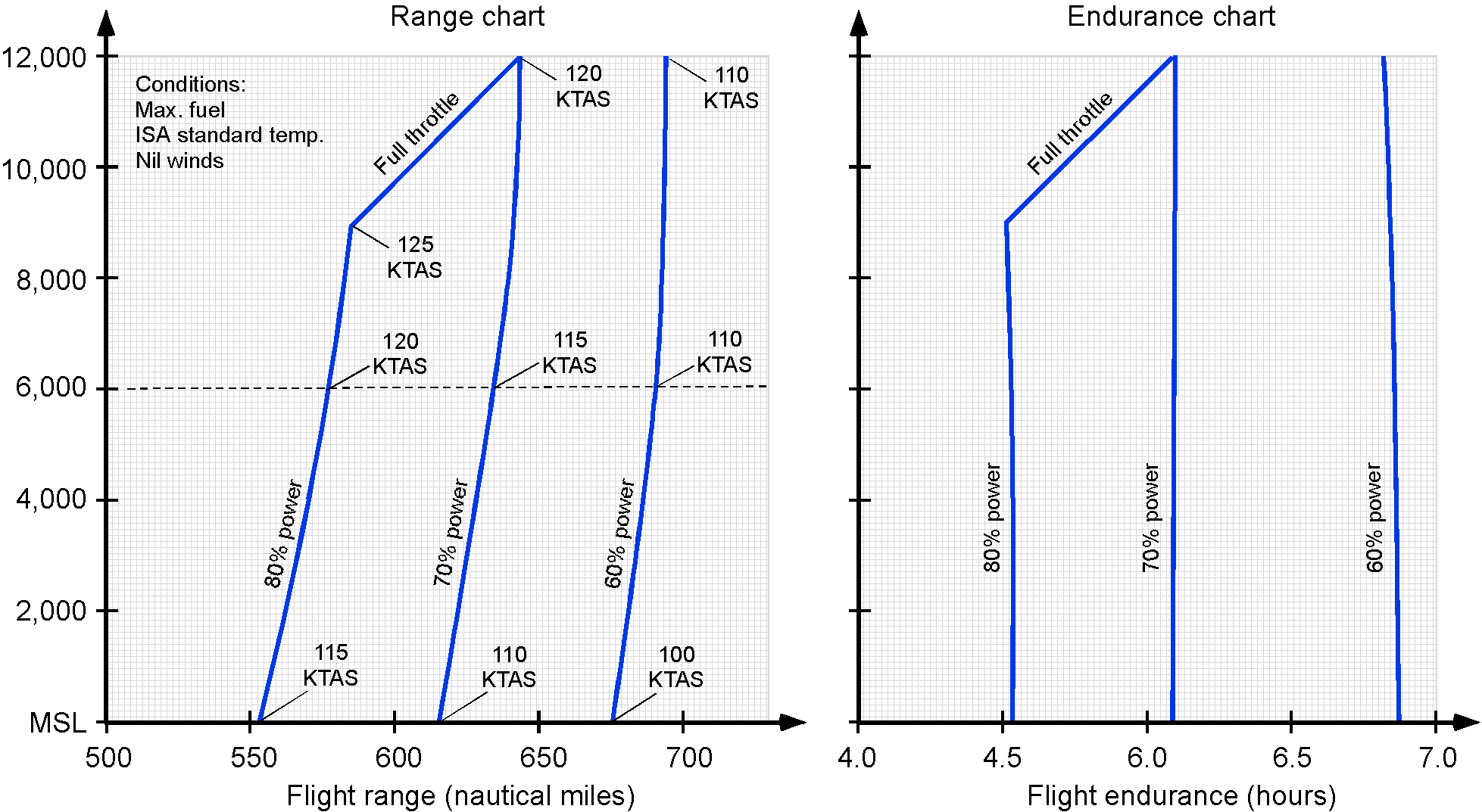
The example below shows a propeller-driven GA aircraft’s range and endurance performance charts. For an airliner, flight endurance is not particularly significant. However, a GA aircraft or drone (with a piston or jet engine) could be used for reconnaissance, surveillance, or other applications where flight endurance is a primary mission requirement. In this regard, range and endurance charts are available for flight planning.
Electric Airplanes
For an electrically powered airplane or drone, both endurance and range are directly derived from the energy stored in the battery and the power required during flight. Unlike a fossil fuel-burning aircraft, the mass of the energy source remains constant during discharge, resulting in straightforward linear relationships.
However, the total energy available for propulsion will not be the full rated capacity of the battery, but the usable fraction remaining after accounting for the allowable depth of discharge (DOD) and any required energy reserve, e.g., for landing and contingencies. If the nominal stored energy is  , the usable energy is
(80) 
where  is the depth-of-discharge fraction (typically 0.8–0.9) and
  is the reserve fraction that must remain at the end of flight for safety or regulatory reasons.
The endurance, or total flight time, is then
(81) 
where  is the power required to sustain the desired flight condition and
  is the overall electrical system efficiency, including the battery, controller, motor, and propeller.
For a steady cruise of a fixed-wing drone, the required power can be written as
(82) 
where is the aerodynamic drag,  is the flight speed, and is the propeller efficiency.
The flight range is the horizontal distance traveled during that time, i.e.,
(83) 
Substituting for for the airplane gives
(84) 
Because the drag can be written as  , this previous result becomes
(85) 
This expression shows that range increases linearly with the stored energy per unit weight and with the aerodynamic efficiency , but is reduced by limits on the depth of discharge and any required reserve fraction. Typical values are  0.8–0.9 and
  0.1–0.2, so the usable energy may be 65–80% of the nominal battery capacity.
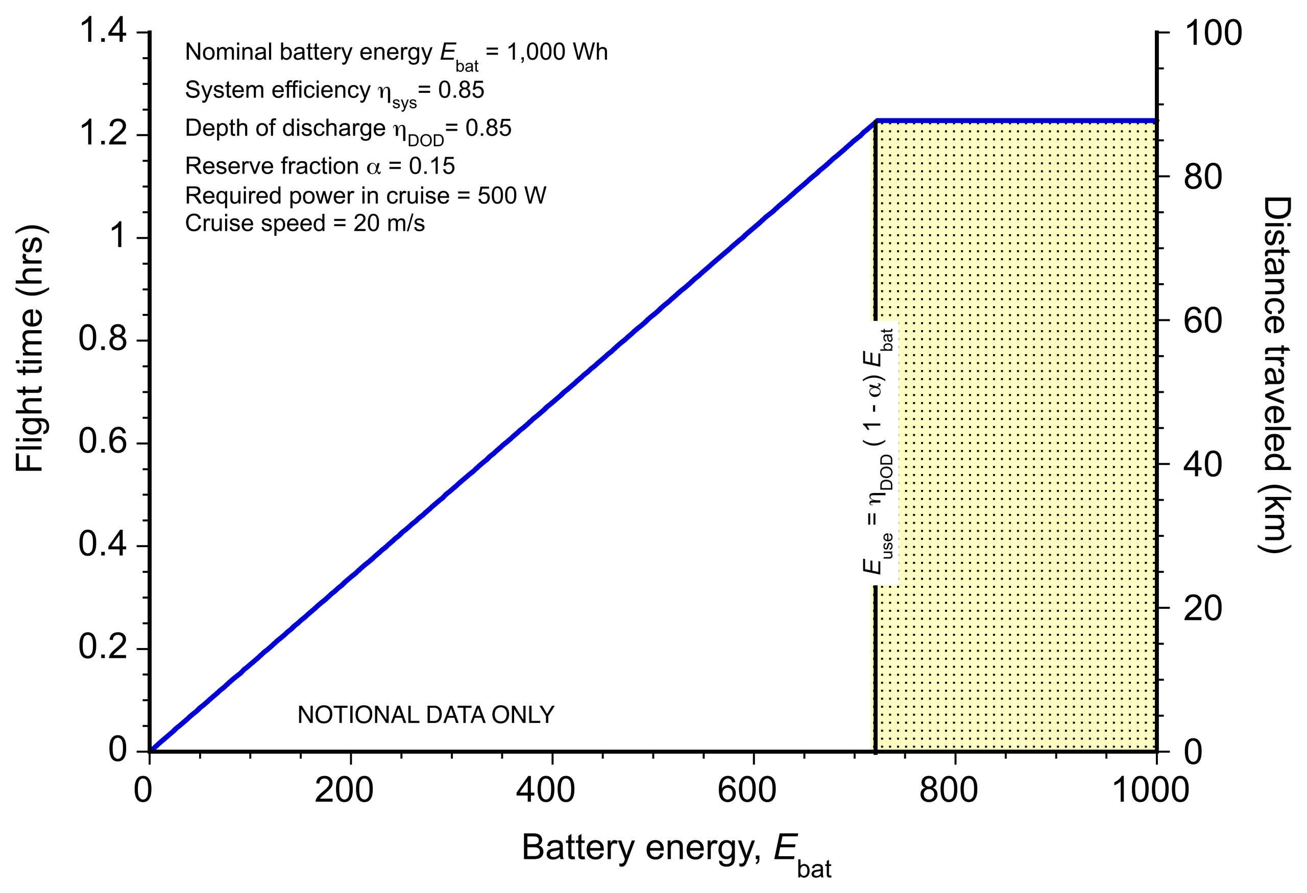
The figure below shows the calculated endurance and range of an electric drone as functions of available battery energy. The nominal stored energy is  1.000 Wh, of which only a fraction is usable after accounting for the depth of discharge
  0.85 and a reserve fraction 0.15. The resulting usable energy is
  722 Wh. With a system efficiency
  0.85, required cruise power
  500 W, and flight speed
  20 m/s, the maximum flight time is about 1.2 hours, and the corresponding range is approximately 87 km. The shaded region beyond
  indicates the energy that cannot be used because of battery discharge and reserve limitations.
The battery energy density, which is typically 200–300 Wh/kg for lithium-ion systems, therefore sets an upper bound on flight time and range. The overall efficiency  usually lies between 0.7 and 0.9. Hovering multirotor drones require significantly higher power because hover power scales approximately with
  , which shortens their flight time relative to fixed-wing aircraft. Environmental factors, including air density, temperature, and discharge rate, will also impact the achievable flight endurance.
Summary & Closure
Estimating flight range (distance) and flight endurance (time) is fundamental to the design process for all aircraft types. In many (most) cases, such as for a commercial airliner, the aircraft’s primary mission is to fly as far as possible on the least fuel and at the lowest cost. In this regard, aerodynamic efficiency (a good lift-to-drag ratio) and engine efficiency (low specific fuel consumption) are critical. The maximum flight endurance is irrelevant for an airliner. However, the flight conditions for the best range are usually at a somewhat lower airspeed relative to the top cruise speed. In practice, an aircraft typically flies at an airspeed slightly above the maximum-range speed to minimize transit time. Military missions often include an element of reconnaissance, which means the airplane is flown to maximize its total time in the air, i.e., at airspeeds that provide the best flight endurance. However, maximizing range and endurance is intrinsically based on engine and aerodynamic efficiency.
5-Question Self-Assessment Quickquiz
For Further Thought or Discussion
- Think of some actual airplane flight profiles or missions where maximum flight range would be essential and where maximum flight endurance would be necessary.
- For a reconnaissance or search mission in a P3 Orion, should the airplane be flown at the airspeed that provides the best range or the airspeed that offers the best endurance? Explain carefully.
- For what type(s) of flight profile or mission would an airplane not be flown at its best range or endurance airspeeds?
- What kind of flight profile (mission) is typically flown by a blimp?
- Explain why the airspeeds to fly for the best endurance or range depend on the airplane’s weight and altitude. Use any equations and/or graphs you think are needed to make the points of your arguments.
- Does the flight range and the speed to fly for the best range depend on the winds? Explain.
- Does flight endurance depend on the winds? Explain.
- When designing a new variant of a jet aircraft, it is desirable to increase the airspeed for optimal range. What steps are necessary to achieve this? Assume operations at the same flight altitude.
Other Useful Online Resources
To dive deeper into fuel burn, flight range, endurance, payload-range charts, etc., check out some of these online resources:
- A video presentation on the payload-range chart.
- An online tutorial on payload-range for a commercial airliner.
- For more background on the calculations of endurance and range, check out the original report, Three Methods of Calculating Range and Endurance of Airplanes, by Walter Diehl.
- To learn more about Louis Breguet and his contributions to aeronautics and aviation, visit the Monash University Hargrave-Andrew Library page.
- The power is measured on a brake dynamometer, which is a mechanical device that provides resistance to the engine shaft. ↵
- Historically, the term engine deck referred quite literally to a deck of punch cards containing the engine performance data supplied by the engine manufacturer to the airframe company. Although those days are long past, the name has persisted. Today, an engine deck is typically delivered as a digital data package or executable program that allows the aircraft manufacturer to model the engine’s performance under various flight conditions and throttle settings. ↵
