37 Classic Airfoil Theory
Introduction
Airfoil theory is a cornerstone of aerodynamics, enabling the prediction of how wing-like shapes, or airfoils, interact with airflows to generate lift and other aerodynamic effects. Many different types of airfoils can be designed with shapes optimized for specific tasks, such as maximizing lift, minimizing drag, or limiting pitching moments. The study of airfoil aerodynamics often encompasses the effects of geometric properties, including camber and thickness distribution, as these properties influence aerodynamic characteristics such as lift, drag, and pitching moment coefficients.
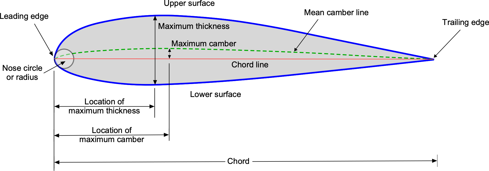
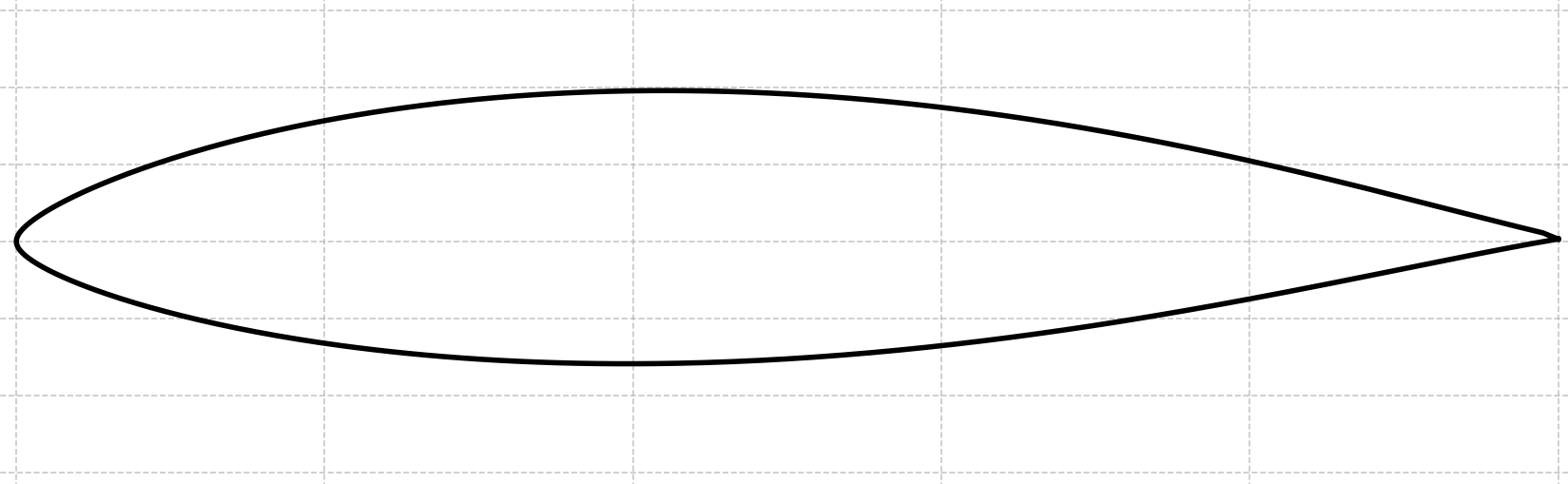
The geometry of an airfoil is described by a profile that defines its upper and lower surfaces, i.e., an envelope, as shown in the figure below. An airfoil section is often called an airfoil profile. The key dimension of an airfoil profile is its size, which is defined in terms of its length or chord, i.e., the distance measured from the leading edge to the trailing edge. The camber of the airfoil profile is a measure of its curvature, which will generally give the airfoil different upper and lower surface shapes. The amount of camber and the chordwise position of the maximum camber strongly influence the airfoil’s aerodynamic characteristics.
The understanding of airfoil section characteristics began with observations and measurements of wings in the wind tunnel, some of the earliest of which were made by the Wright brothers. The Wrights were surprised that no aerodynamic theory existed in 1900, but at that time, aerodynamics was not yet considered a serious scientific discipline. However, the aerodynamic theory would soon catch up by the 1920s and evolve into increasingly sophisticated predictive capabilities. Among the most influential analytical models were the conformal transformation technique, which led to the development of the so-called Joukowsky airfoils, and subsequently, to the thin airfoil theory.
The method of conformal transformation is a classic approach in two-dimensional aerodynamic theory, exposing a direct link between the geometry of an airfoil and its aerodynamic behavior. Specifically, the Joukowsky transform of the canonical flow about a circle into an airfoil shape with a cusped trailing edge demonstrates how angle of attack, chordwise curvature (i.e., camber), and thickness distribution influence the pressure distribution and lift generation. The thin-airfoil theory emerges naturally as a limiting case of this approach, where the airfoil thickness and camber become infinitesimally small. Despite its relative analytical simplicity, the thin airfoil theory provides essential insights into airfoil behavior. It also serves as a foundation for more complex aerodynamic analyses, including applications to subsonic and supersonic flows and to unsteady aerodynamic behavior.
While it may take some time for new engineers to fully appreciate the depth and insight offered by these classic airfoil theories, all students of aerodynamics must engage with them early on as a foundational part of their education and training. Through these approaches, they will gain a deeper understanding of fundamental aerodynamic principles, the connection between airfoil geometry and aerodynamic performance, and develop essential skills in mathematical modeling and problem-solving that carry over into practical engineering applications and research endeavors.
Learning Objectives
- Be able to explain conformal transformations and apply them to map potential flows about a circular cylinder onto airfoil-shaped boundaries.
- Understand and describe the role of vortex sheets in aerodynamic theory.
- Recognize and assess the assumptions and simplifications underlying thin airfoil theory.
- Derive and interpret key equations governing airfoil performance, including lift and pitching moment.
- Use thin airfoil theory to predict the aerodynamic characteristics of an airfoil with a specified camberline.
- Apply classical airfoil theory to design airfoil shapes that meet defined aerodynamic performance goals.
History
Contributions from several aerodynamic pioneers shaped the development of what is known today as the classic airfoil theories. The foundations were laid by Isaac Newton in his Principia in 1726, where he proposed an early impact theory of air resistance, an approach limited by its neglect of fluid continuity and circulation. Newton predicted that the lift coefficient,  , depended on the sine square of the angle of attack, i.e.,
  , which others subsequently showed was an inadequate comparison to measurements, as presented in the schematic below.
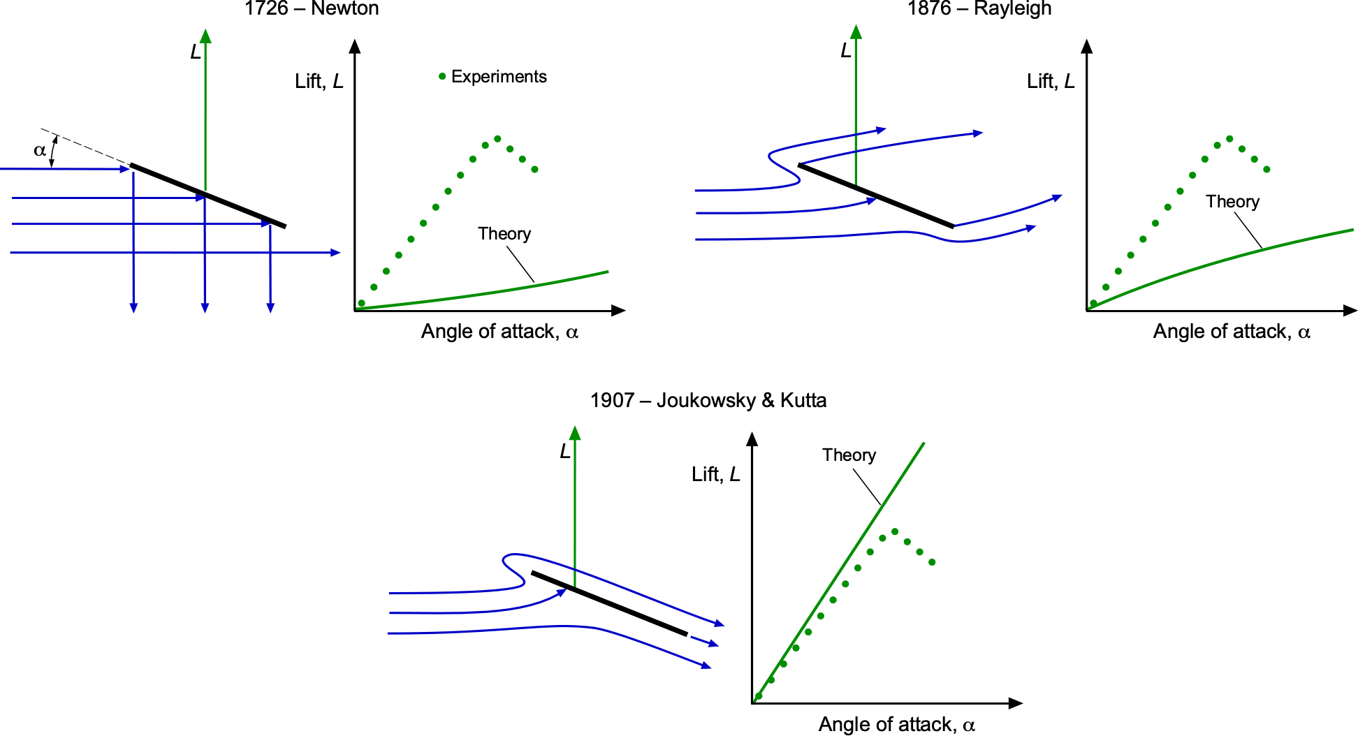
Later, Lord Rayleigh, in his 1876 Publication of “The Theory of Sound,” formalized the mathematical basis for potential flow, providing a foundation for later aerodynamic theory. However, his lift formula, given by  still significantly underpresented the measured lift. Frederick W. Lanchester was among the first to propose a physical explanation for lift, introducing the concept of circulation. A few years later, Ludwig Prandtl, often regarded as the father of modern aerodynamics, laid the groundwork for understanding flows over airfoils. Prandtl’s concurrent work on boundary layers and viscous effects also laid the groundwork for understanding the interplay between inviscid theory and real fluid behavior, paving the way for rapid advances in aerodynamic modeling in the early 20th century.
Historically, the first published application of aerodynamic theory for two-dimensional airfoils was the conformal mapping method, which was used to obtain the solution for the flow around an airfoil, much of which is attributed to Martin Kutta (also known as Wilhelm Kutta). In his 1902 paper,[1] Kutta mapped the potential flow around a circular cylinder onto a flat plate set at an angle of attack to the flow, imposed a finite velocity at the trailing edge based on experimental observations (now called the Kutta condition), and derived the  lift formula that is a key part of the Kutta-Joukowsky theorem. A few years later, Nikolai Zhukovsky (Joukowsky) generalised the technique[2] to convert a suitably placed circle into a finite-thickness, cusped airfoil profile, now known as the classic Joukowsky airfoil.
An asymptotic expansion of the conformal-mapping solution linearises the surface boundary condition to the mean camber line of an airfoil. As will be shown, this approach leads to a first-order singular integral equation for the bound vortex-sheet strength, which must be solved subject to flow tangency on the camberline. This linear equation, together with the Kutta condition of zero sheet strength at the trailing edge, constitutes the essence of the thin-airfoil theory. From this, several classical results emerge that confirm those from the more general potential-flow solution obtained via the conformal transformation approach.
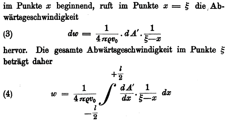
The mathematical formulation of thin airfoil theory was first advanced by Max Munk, a Ph.D. student of Ludwig Prandtl, who introduced the concept of representing airfoil lift using vortex sheets. Munk’s contribution[3] established the connection between the lift force and the shape of the camberline of an airfoil, which is central to thin airfoil theory. The extract shown in the figure below from Munk’s 1909 dissertation establishes what is now known as the fundamental equation of thin-airfoil theory, based on the principles of vortex sheets and the Biot-Savart law.
Later mathematical developments and refinements to the thin airfoil theory by Hermann Glauert[4] made the theory more practical for routine use by using a general Fourier series approach to represent an arbitrary chordwise aerodynamic loading. Munk’s analysis, as Glauert stated, “is not quite free from errors,” so Glauert presented a more careful analysis with both mathematical and practical rigor. The aerodynamics of airfoils with arbitrary camber can then be analyzed, with many valuable applications.
In the 1930s, Theodore Theodorsen extended the thin airfoil theory to unsteady aerodynamic problems, such as oscillating airfoils, thereby fostering the development of other aerodynamic theories for non-steady flows applicable to aeroelasticity and flutter problems. It is noteworthy that the NACA family of airfoil shapes, as previously discussed, which have become iconic in airplane design, used the principles underlying the thin airfoil theory, thereby highlighting the lasting impact of this theory in the field of aeronautical engineering.
Force & Moment Conventions
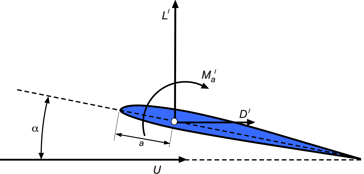
Before proceeding, a reminder of the aerodynamic coefficients acting on an airfoil section at an angle of attack  is appropriate. The lift force per unit length (span),
  , acts in a direction perpendicular to the freestream velocity,
  , or
, or  in the convention of the classic thin airfoil theory, as shown in the figure below. The corresponding drag per unit span,
  , is parallel to , and there is also a moment
  about the point where the lift and drag are assumed to act. In a potential flow, the drag is zero, a result known as D’Alembert’s paradox.
The dimensionless force coefficients are defined using the freestream dynamic pressure,  , and chord,
  , as a reference, i.e., the lift coefficient, , and the drag coefficient,
  , are given by[5]
(1) 
where the freestream dynamic pressure is  . For an incompressible flow,
  at all points, so the
  subscript can be dropped. Likewise, can be used to denote
  .
.
Pitching moments on an airfoil can be resolved to any convenient reference point, as shown in the figure below. The dimensionless moment coefficient for an airfoil section can be defined as
(2) 
where  is some moment axis location. The 1/4-chord axis position is the most common, so that
(3) 
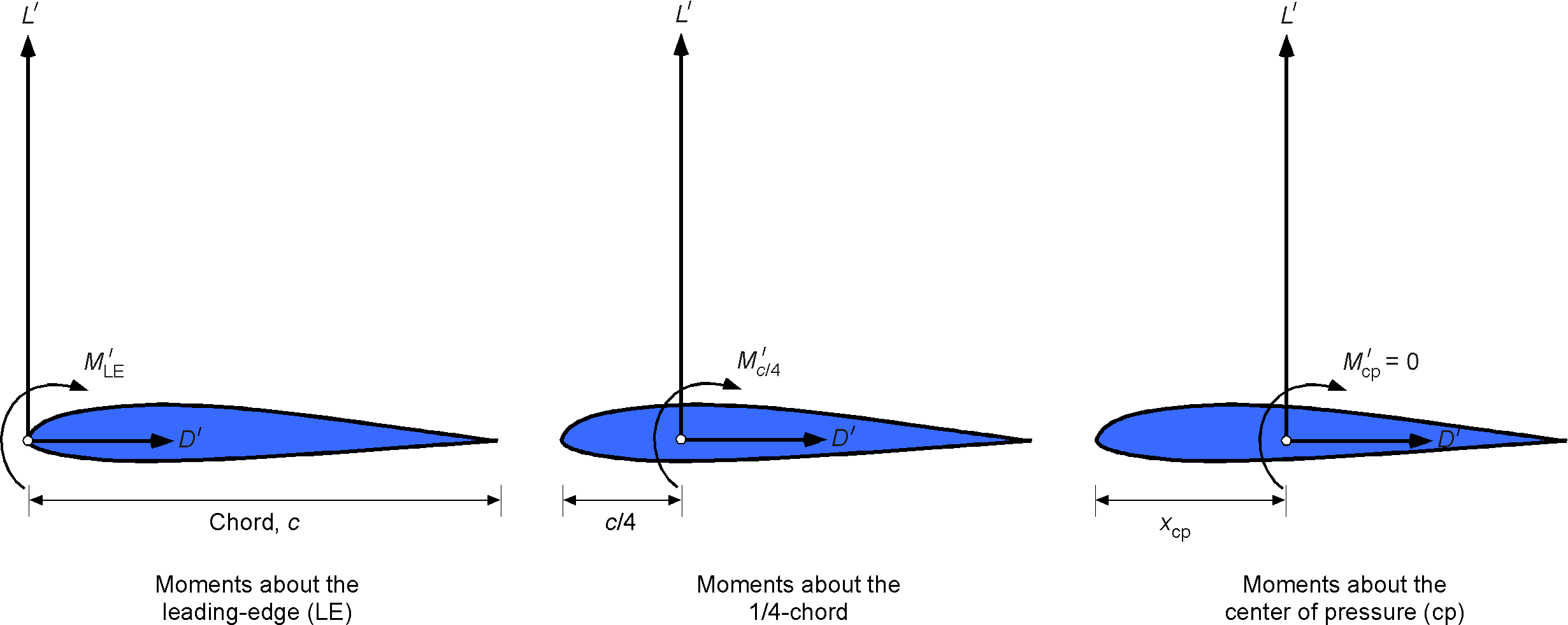
Pitching moments may be taken about any axis, but the 1/4-chord is the most common. However, the moment about any axis point can be obtained using the principles of statics. In practice, one should double-check which axis the moments are calculated with respect to.
Kutta Condition
To understand the classic airfoil theories, it is first necessary to understand the physics of the Kutta condition. The Kutta condition is based on the empirical observation that the flow leaves the trailing edge of an airfoil smoothly, without singularities in the velocity or static pressure. As an empirical observation, it must be incorporated into the classical airfoil theories. This condition was demonstrated in the early experiments of Prandtl and Teitjens, who, about 1910, visualized the flow around an impulsively started airfoil at an angle of attack, as shown below; watch the historical film here. Since then, many investigators have conducted confirmatory experiments of the Kutta condition at higher flow velocities and Mach numbers.
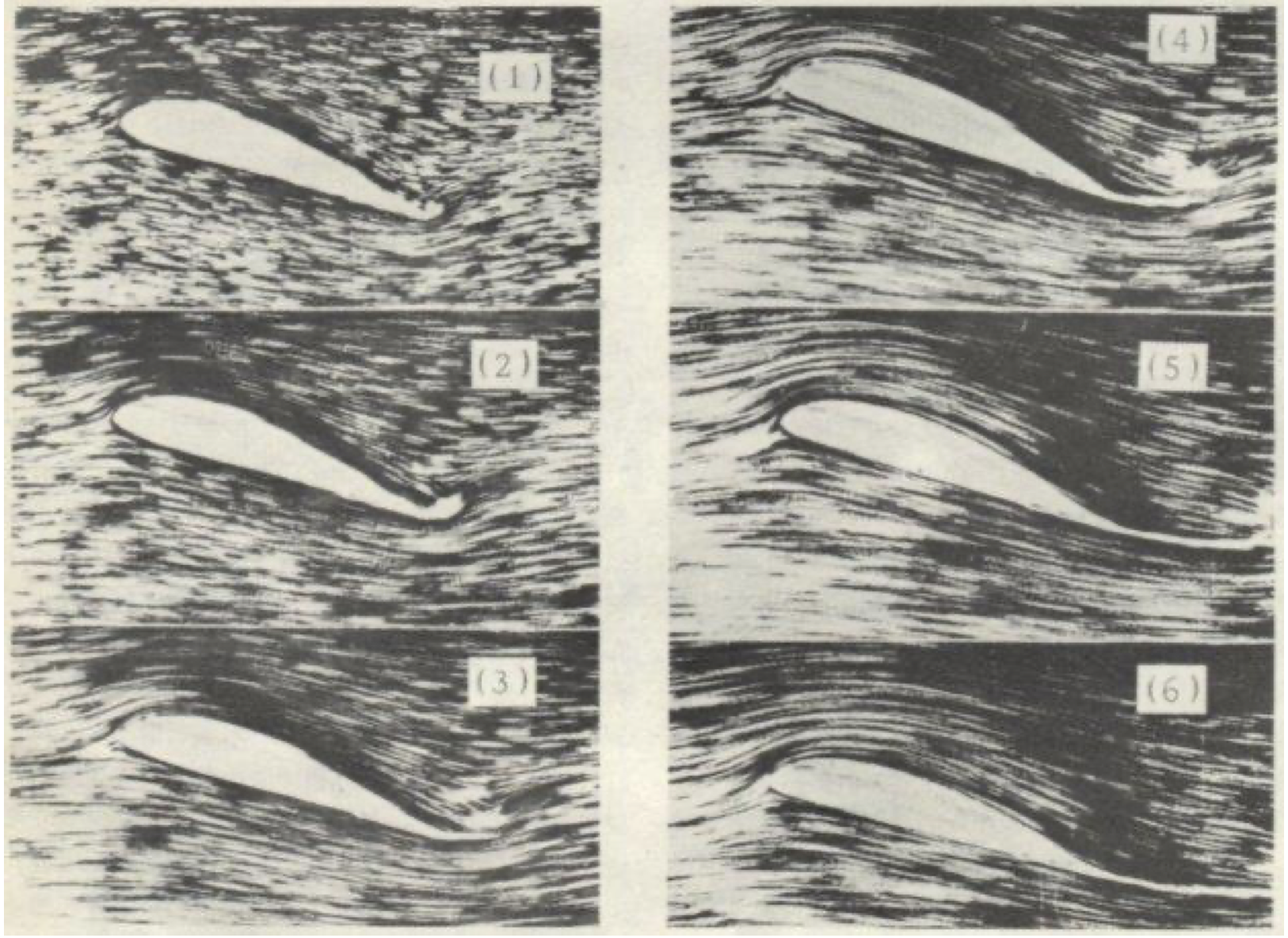
As shown in Frame (1), the initial flow establishes, causing a local vortex and circulation around the trailing edge that extends toward the upper surface. Still, no significant circulation or lift is generated on the airfoil at this stage. As the flow first curls around the trailing edge, locally high velocities and low pressure are obtained.[6] which are not sustained for very long. Frames (2) through (5) then depict the temporal development of a starting vortex, which forms and is shed from the trailing edge as the flow continues to evolve. During this time, circulation increases and lift builds. In frame (6), the steady-state flow is fully established, leaving the trailing edge smoothly in accordance with the Kutta condition, and full lift is achieved. The initial vortex is convected downstream asymptotically. It will eventually not influence the flow at the airfoil so that it can be disregarded in any steady-state flow analysis[7].
Starting Vortex & Kelvin’s Theorem
Kelvin’s circulation theorem is closely connected to the concept of the starting vortex and the Kutta condition. This theorem states that circulation in a potential flow is conserved and can be described mathematically as
(4) 
Understanding the concept of circulation requires some thought, along with the connection of circulation to lift generation on a body in motion. Consider an airfoil initially at rest. If  , the circulation
  about the circuit around the airfoil must also be zero. When the airfoil is set into motion, it develops a nonzero circulation
  , as shown in the figure below. Observations of this flow show that a starting vortex with a counter circulation
  is shed from the trailing edge. This shedding also satisfies the Kutta condition at every instant in time. The vortex is swept downstream, as observed in the standard reference frame moving with the airfoil. In the steady state, it is convected to infinity with no influence.
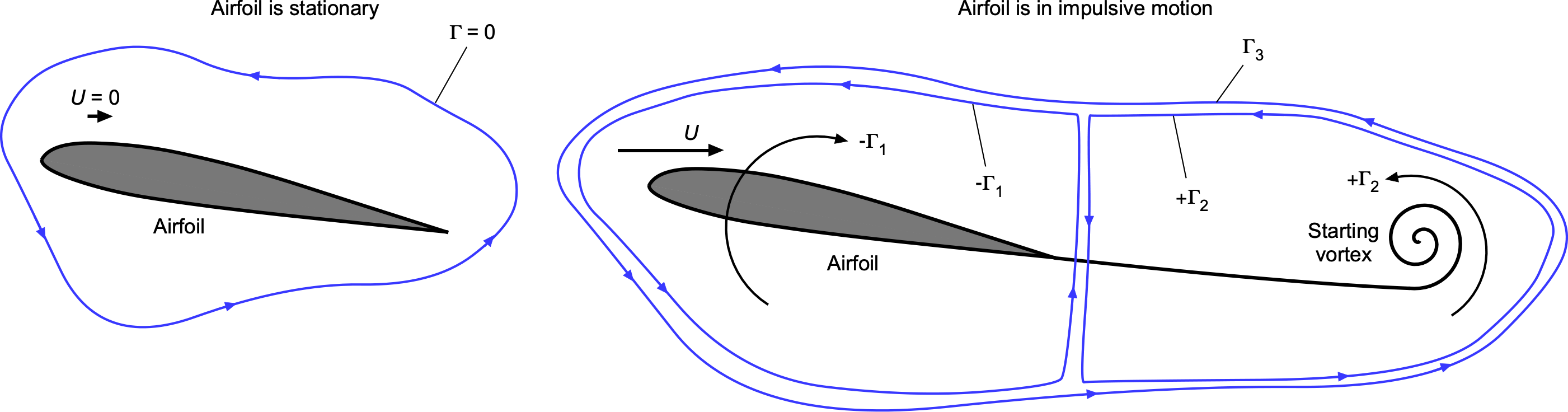
Following Kelvin’s theorem, the overall circulation  must be zero and so equal the sum of the airfoil circulation and the shed vortex circulation, i.e.,
(5) 
Therefore, regardless of the sign convention, the airfoil and the starting vortex must have equal and opposite values of circulation, i.e.,
(6) 
As previously noted, a longer time[8] after the start of motion, the starting vortex is far downstream behind the airfoil and has no influence on the flow field around the airfoil. Therefore, the shed starting vortex can be disregarded when considering steady 2-dimensional airfoil flows. However, the continuous shedding of circulation into the near wake must still be considered in unsteady airfoil flows, as this creates an induced velocity that affects the instantaneous circulation around the airfoil and, hence, its lift.
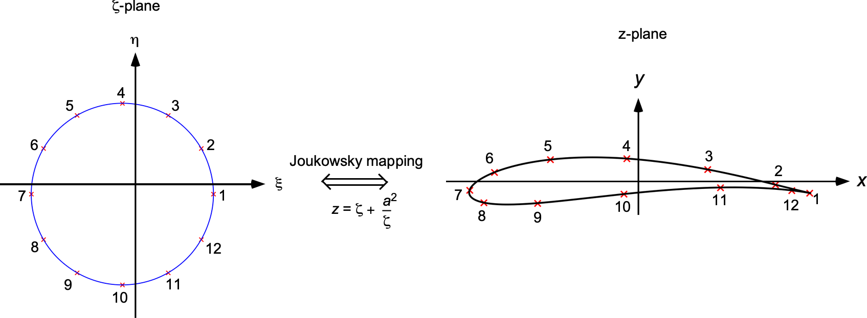
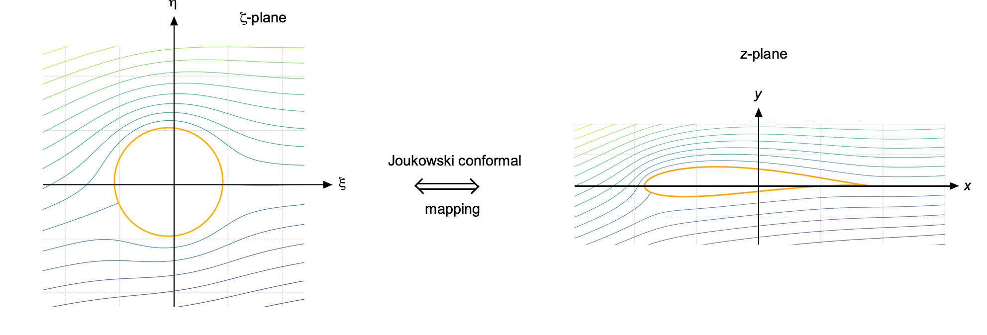
Conformal Transformations & Joukowsky Airfoils
Most engineers find the conformal-transformation approach and the derivation of the classical Joukowsky airfoil results to be quite challenging to understand. It is therefore advisable for the student to revisit the previous chapter on potential flows and refresh the basic method of conformal mapping; if needed, a review of the underlying complex‐analysis methods can also be undertaken. On a first reading, one may even choose to defer the detailed airfoil‐mapping derivation and proceed directly to the discussion on thin‐airfoil theory, which can be studied in isolation. Nonetheless, the conformal-transformation framework provides the fundamental justification for all the assumptions and results in the thin-airfoil theory. So it ultimately underpins a rigorous understanding of how the angle of attack and camber will influence lift generation.
A conformal mapping is an analytic transformation, say  that transforms each point given by
  in one complex plane to a new point
  in another plane, while preserving the local angle between intersecting functions and curves. Because conformal mappings preserve harmonicity, any velocity potential or stream function satisfying Laplace’s equation in the
  -plane also satisfies it in the
  -plane. This property allows the construction of an aerodynamic flow solution in two steps. 1. Solve the potential flow around a known canonical geometry in the -plane. 2. Apply an appropriate conformal transformation
  to map that solution onto a boundary in the -plane, thereby obtaining the new potential flow field for another, and inevitably, more complicated flow problem. For example, the classic Joukowsky conformal transformation maps a circular cylinder (circle) in the -plane onto an airfoil shape in the -plane, i.e., using
(7) 
as shown in the figure below.
Lifting Circular Cylinder
Now, the lifting Joukowsky airfoil problem must be considered. In this case, circulation must be produced about the airfoil, which is set by the angle of attack with respect to the flow and the imposition of the Kutta condition that the flow leaves the trailing edge smoothly and without discontinuity in velocity or pressure. In the plane, the development of the Joukowsky airfoil flow starts with a circular cylinder of radius centered at
![\[ \zeta = \zeta_0 = \xi_0 + i\,\eta_0,\quad |\zeta_0| \le a \]](https://eaglepubs.erau.edu/app/uploads/quicklatex/quicklatex.com-8cf99da3390455dfb1a4bbd4856ed394_l3.svg "Rendered by QuickLaTeX.com")
That is immersed in a uniform freestream. The flow is now set at an angle  , and circulation is developed. This flow has a complex potential in the -plane given by
(8) 
Notice that  =
=  represents the effects of thickness and camber on the shape of the Joukowky airfoils.
Notice that under a conformal mapping, the complex potential itself is unchanged and is re-expressed as the same function in different variables. So if  in the -plane, then
  leads to the identical potential and stream function in the -plane.
To find the velocity field, the derivative of the potential function is
(9) 
so that
(10) 
Using the chain rule to get the complex velocity field in the -plane leads to
(11) 
Joukowsky Flow
The shape of the Joukowsky airfoil profiles has already been explained: the points on the circle map are mapped to points on the airfoil. The points on the cylinder in the plane are
(12) 
and the tangential velocity there, with circulation now being imposed, is
(13) ![\begin{equation*} V_\theta(\theta) =\Re\Biggl\{ -\,i\;\biggl[ U\,e^{-i\alpha}\left(1 - \frac{a^2}{(\zeta(\theta)-\zeta_0)^2}\right) +\frac{i\,\Gamma}{2\pi\,(\zeta(\theta)-\zeta_0)} \biggr]\; \frac{\zeta(\theta)-\zeta_0}{\lvert\zeta(\theta)-\zeta_0\rvert} \Biggr\} \end{equation*}](https://eaglepubs.erau.edu/app/uploads/quicklatex/quicklatex.com-090339f6bc51c1ba6ff8ccb95af5ef2b_l3.svg "Rendered by QuickLaTeX.com")
Under the mapping  the airfoil shape in the -plane is
(14) 
Notice that starting from the transformation
(15)
the leading‐edge and trailing‐edge of the airfoil correspond to the points  , i.e.,
(16) 
so that the physical chord runs from  to
to  , giving
(17) 
Strictly speaking, for a circle of radius centered at the origin, the mapped chord length is  . However, many texts define the reference circle using
  and place the trailing edge at
  , so that the mapped chord length is taken to be
  by construction.
More generally, if the circle is offset from the origin by a complex amount , then
(18) 
and the leading and trailing edge locations become
(19) 
so the chord length depends on both and  . But for thin-symmetric or mildly cambered airfoils, it remains acceptable in practice to adopt for scaling purposes, and this approximation is mostly used in what follows.
Velocity Field
The various shapes of the Joukowsky airfoils are best illustrated by their effects on the velocity field and pressure distribution. In this regard, the Kutta condition must be specifically imposed at the trailing edge. The trailing‐edge cusp occurs where
(20) 
which gives
(21) 
Choosing the downstream solution  , the complex velocity must be
(22) 
to remain finite at the cusp. Therefore,
(23) 
The complex potential in the -plane is
(24) 
so the corresponding complex velocity is
(25) 
Substituting into this expression gives
(26) 
Hence, the velocity remains finite only if  , which corresponds to symmetric flow with no lift. Therefore, a nonzero circulation cannot satisfy the Kutta condition unless the trailing edge is located at a different point on the circle.
To obtain a cusped airfoil with nonzero circulation, the generating circle must be displaced from the origin. In this case, the trailing edge corresponds to the point
(27) 
where  is the angle defining the offset of the circle center from the real axis. Applying the Kutta condition at this point gives
(28) 
which ensures a finite velocity at the trailing edge and determines the circulation required for lift.
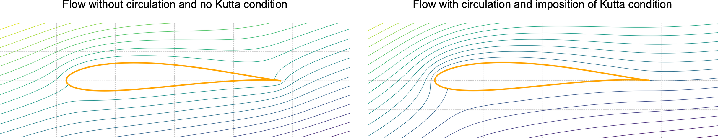
The beauty of the Joukowsky transformation lies in its ability to map the canonical solution of potential flow around a circle to the flow around an airfoil, as illustrated in the figure below. This approach preserves the essential features of lift-generating flows while enabling an analytic treatment of more realistic shapes.
Role of the Kutta Condition
In airfoil theory, the Kutta condition is foundational in ensuring that the mathematical solution corresponds to a physically realizable flow. For airfoils with a sharp trailing edge, such as those derived from the Joukowsky transformation, the potential flow equations alone are insufficient to determine the flow uniquely. Without an additional constraint, the circulation around the airfoil remains undetermined, and the solution is physically incomplete. Consequently, there is no lift. Moreover, the velocity at the trailing edge becomes infinite, revealing a nonphysical singularity in the solution. This case, although mathematically valid, does not accurately represent the behavior of an airfoil in a viscous flow.
Explicitly imposing the Kutta condition resolves this ambiguity. It specifies that the flow must leave the sharp trailing edge smoothly, with finite velocity, as illustrated in the figure below. This requirement is motivated by both experimental observation and boundary-layer theory, which shows that viscous effects drive this behavior. In potential flow models, this constraint must always be imposed, allowing the circulation to be determined uniquely. When the Kutta condition is imposed, the velocity remains finite throughout the flow field, and, except at the trailing edge, a net pressure difference appears between the upper and lower surfaces of the airfoil, thereby producing lift.
 = 0, and with a finite circulation imposed by the mathematical imposition of the Kutta condition.
The corresponding lift on the airfoil is given by the Kutta-Joukowski theorem, i.e.,
(29) 
Substituting the expression for the circulation that satisfies the Kutta condition gives
(30) 
The chord length of the Joukowsky airfoil is  , so the lift coefficient is
(31) 
This result shows that the lift depends not only on the angle of attack , but also on the camber, which is represented by angular displacement that defines the offset of the generating circle in the -plane. For small values of and , the expression reduces to
(32) 
which is a classic result in airfoil theory. It predicts that the lift coefficient is proportional to the angle of attack, i.e., a linear relationship, a fact confirmed by experiments with airfoils and wings.
Parametric Variations
For a zero offset = 0 with  = 0 and
  = 0, the transformation produces a flat plate with zero thickness. However, by choosing the offset
  with
with  , the camber and trailing‐edge shape of the resulting Joukowsky airfoil can be controlled, all while preserving the analytic potential flow solution using a single substitution. In this regard, a series of parametric variations in angle of attack, thickness, and camber can be used to examine the effects on the resulting flowfield about Joukowsky airfoils.
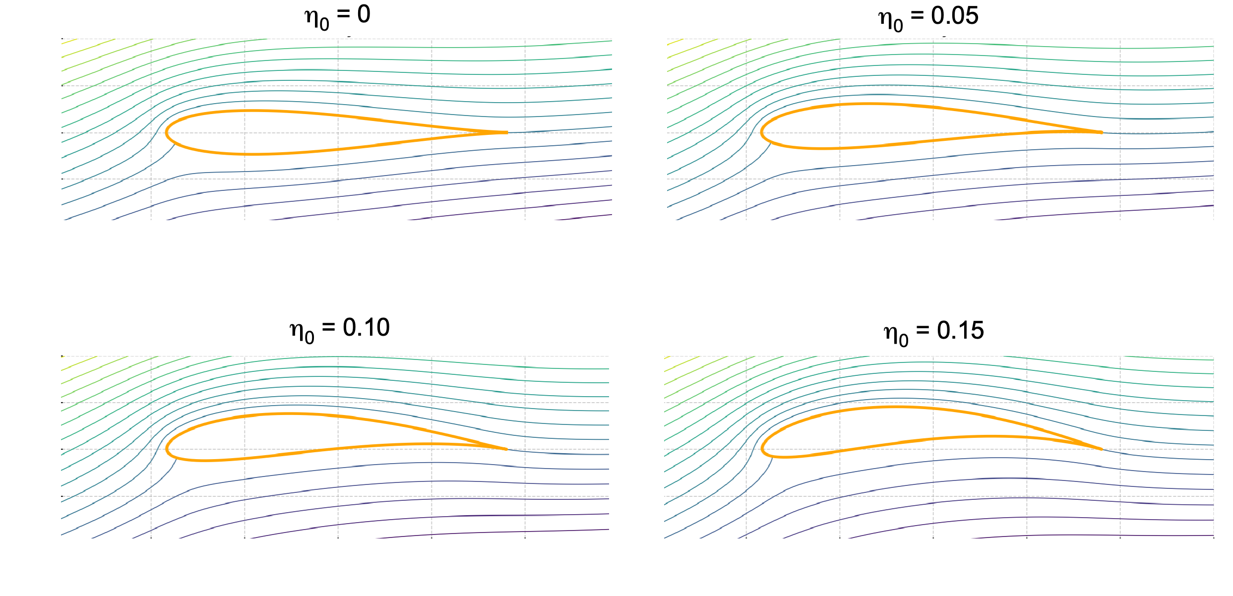
Effects of Angle of Attack
The effects of angle of attack are shown in the figure below. At zero angle of attack, which is measured here as the apparent inclination of the streamlines relative to the airfoil, rather than a rotation of the airfoil in a fixed freestream, the flow passes smoothly over both the upper and lower surfaces, and the streamlines are relatively widely spaced. By definition, an equal mass flow lies between successive streamlines, so where they converge, the local velocity must increase.
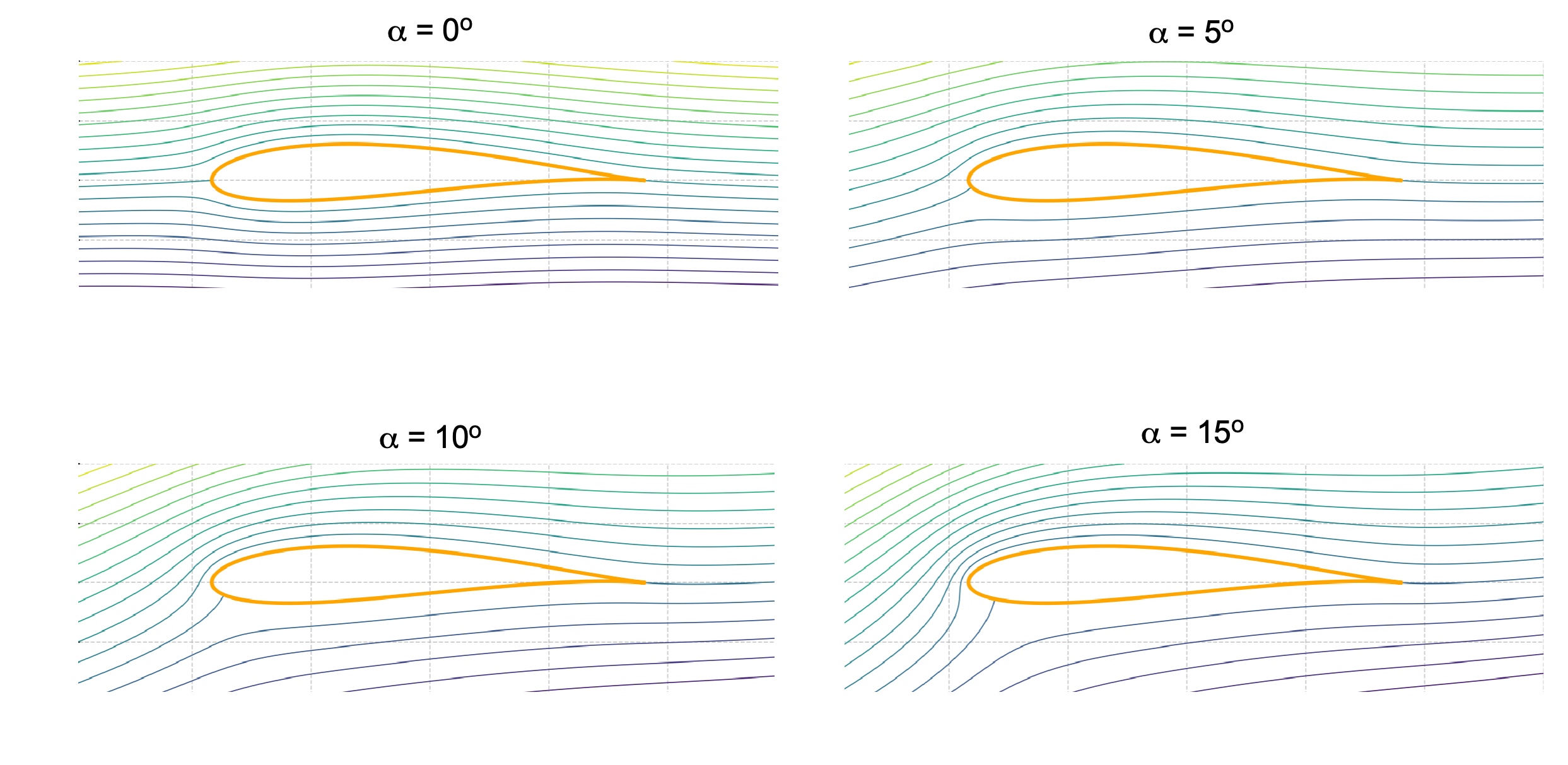
As the nominal angle of attack is increased to 10o, the streamlines ahead of the leading edge and in particular those over the upper surface bunch more tightly, while those beneath the airfoil spread apart. This result indicates a rise in velocity (and so a drop in pressure according to the Bernoulli principle) over the upper surface and a corresponding deceleration (and pressure rise) below. The region of tightest convergence is immediately at the nose, showing that most of the low-pressure (and hence lift-producing) action remains concentrated near the leading edge. At 15o, the upper‐surface streamlines crowd even more strongly at the nose and leading‐edge region, while the lower‐surface patterns move farther away. The resulting pressure differential grows, driving a further increase in lift.
In the classical formulation of potential flow about a Joukowsky airfoil, the angle of attack is introduced by rotating the direction of the freestream velocity vector. Rather than physically rotating the airfoil geometry, the freestream is expressed as a complex exponential  where is the freestream speed and is the angle of attack measured in radians. This representation corresponds to a clockwise rotation of the flow by an angle in the complex plane. This approach maintains the airfoil geometry fixed in the physical -plane, with the trailing edge aligned along the real axis. This alignment is essential for applying the Joukowsky transformation. By rotating the freestream rather than the airfoil, the angle of attack is introduced relative to the airfoil chord line, and the Kutta condition can be applied directly at the trailing edge. This technique preserves the solution’s analytical tractability while correctly modeling lift generation through circulation.
Effects of Thickness
As shown in the figure below, a -offset in the -plane introduces thickness into the mapped airfoil profile without altering its symmetrical shape about the chord line. At a fixed 0o nominal angle of attack, increasing the maximum thickness of the section causes a noticeably stronger curvature of the streamlines and a tighter clustering immediately ahead of the leading edge. The effects produced, however, even for a cambered airfoil, are nominally symmetric between the top and bottom airfoil surfaces, thereby producing no significant changes in lift or pitching moment. Notice that these cases represent significant changes in the thickness-to-chord ratio compared to any practical airfoil, and are selected to over-emphasize the effects of thickness.
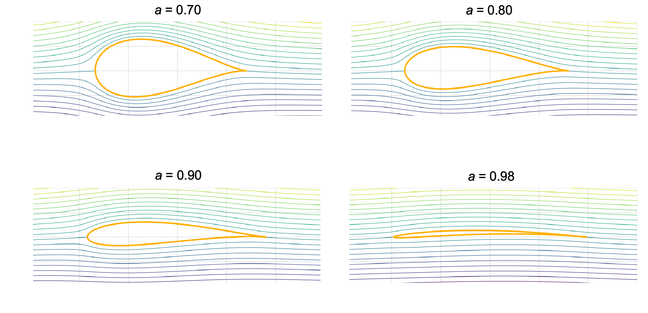
Thicker bodies disturb the flow more, but the thickness‐induced changes are quite modest compared to those produced by varying the angle of attack or the camber. As the section becomes ever thinner, the flow perturbations diminish in the limit of a vanishing thickness (i.e., a flat plate), the only significant super-velocities are at the leading edge, seen in the slightly close streamline spacing there, while the remainder of the surface experiences almost freestream conditions with only minor deviations.
Effects of Camber
A combined  -axis and
  -axis offset, i.e.,
  , in the -plane skews the airfoil contour and streamlines in the -plane, giving the Joukowsky airfoil both camber and thickness asymmetry, as shown in the figure below. The stagnation points shift chordwise and/or vertically, demonstrating the control over the airfoil shape and its flow that results from displacements of the circle center in the -plane.
Camber modifies the pressure distribution in much the same way as increasing the angle of attack, and its aerodynamic influence is generally more significant than the effects of thickness. By curving the mean line of the section, camber effectively increases the local angles seen by the oncoming flow, producing correspondingly higher lift. Conversely, to achieve a given lift level, a cambered section must be set at a lower geometric angle of attack than a symmetric one.
The particular angle of attack at which a cambered airfoil generates zero net lift is known as the zero-lift angle of attack, often denoted by  ; its value is always negative for a positively cambered section, typically between -1o and -2o. In practice, it serves as a useful baseline when comparing different camber lines, and the lift coefficient at a given angle of attack can be referenced back to this zero-lift datum.
Pressure Coefficient Distribution
On the circular cylinder in the -plane, the surface is defined by the polar surface
(33) 
The surface velocity is
(34) 
and splitting it into Cartesian components gives
(35) 
The corresponding pressure coefficient on the surface of the airfoil is then obtained from
(36) 
Effects of Angle of Attack
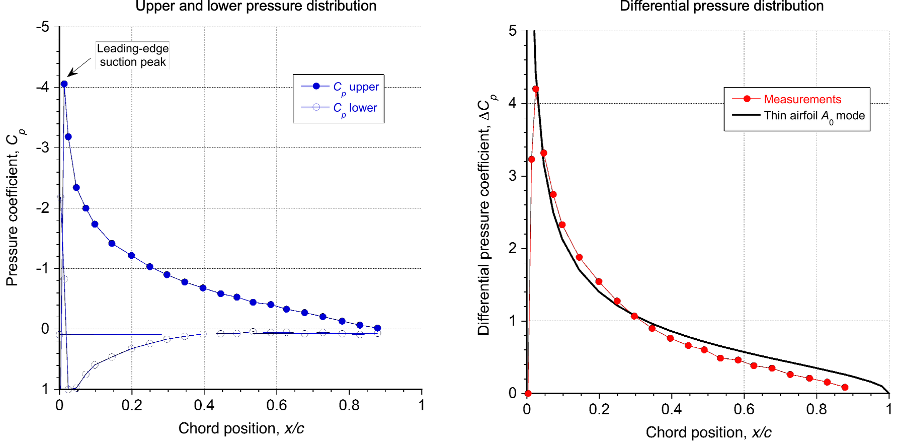
Representative results for changes in angle of attack are shown in the figure below. As the angle of attack increases, the pressure distribution over the airfoil undergoes significant changes. At 0o, there is a minimal pressure difference between the upper and lower surfaces, resulting in negligible lift. At an angle of attack of 5o, leading-edge suction begins to develop on the upper surface, and the stagnation point shifts from the nose to the lower surface near the leading edge. As the angle increases further to 10o a pronounced suction is evident on the upper surface, with the stagnation point moving further aft along the lower surface. This progression enhances the pressure difference, generating a noticeable lift. By 15 °, the pressure difference between the upper and lower surfaces becomes substantial, producing significant lift.
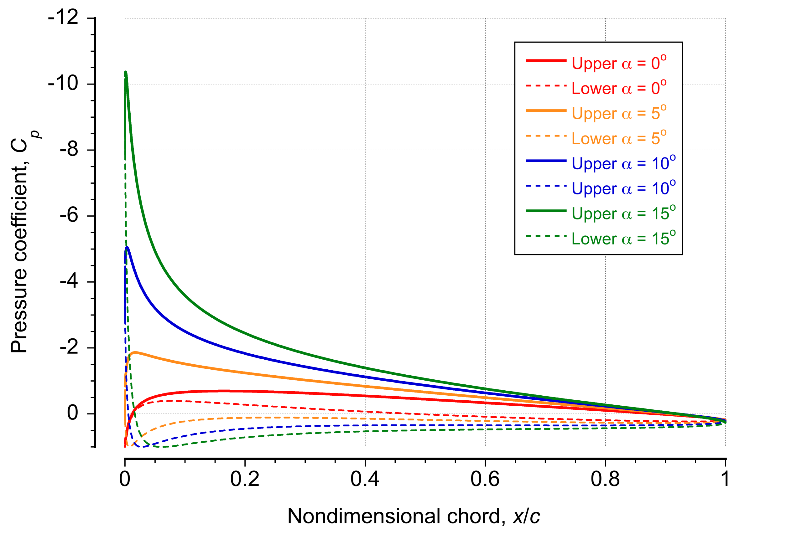
 versus chordwise position
  for a Joukowsky airfoil with offsets
  and
and  .
.The resulting pressure distributions can also be integrated to find the lift and the pitching moment about some convenient point. This process must be performed numerically with the mapping of discrete points from the surface of the circle in the -plane to the airfoil surface in the plane. However, results for lift and pitching moment can also be obtained analytically, as discussed in the next section, which highlights the key characteristics of airfoils as they change with angle of attack and camber.
Effects of Thickness
A significant advantage of an exact airfoil theory is its ability to examine the effects of airfoil shape on the pressure distribution and, ultimately, on lift and moment behavior as functions of angle of attack. For example, in the figure below, the effects of airfoil thickness for a given amount of camber at an angle of attack of five degrees are illustrated. Notice that the effects of thickness are relatively small. Although a thicker airfoil introduces some camber to the flow, the differences in pressure distribution between the upper and lower surfaces remain modest. This implies that thickness may influence the lift and moment characteristics. Still, relative to the effects of angle of attack and geometric camber, these influences tend to be small, at least within the small range of thickness-to-chord ratios found in practical airfoil sections. Nonetheless, experimental measurements suggest that airfoils with greater thickness tend to exhibit very slightly higher lift coefficients and slightly steeper lift curve slopes.
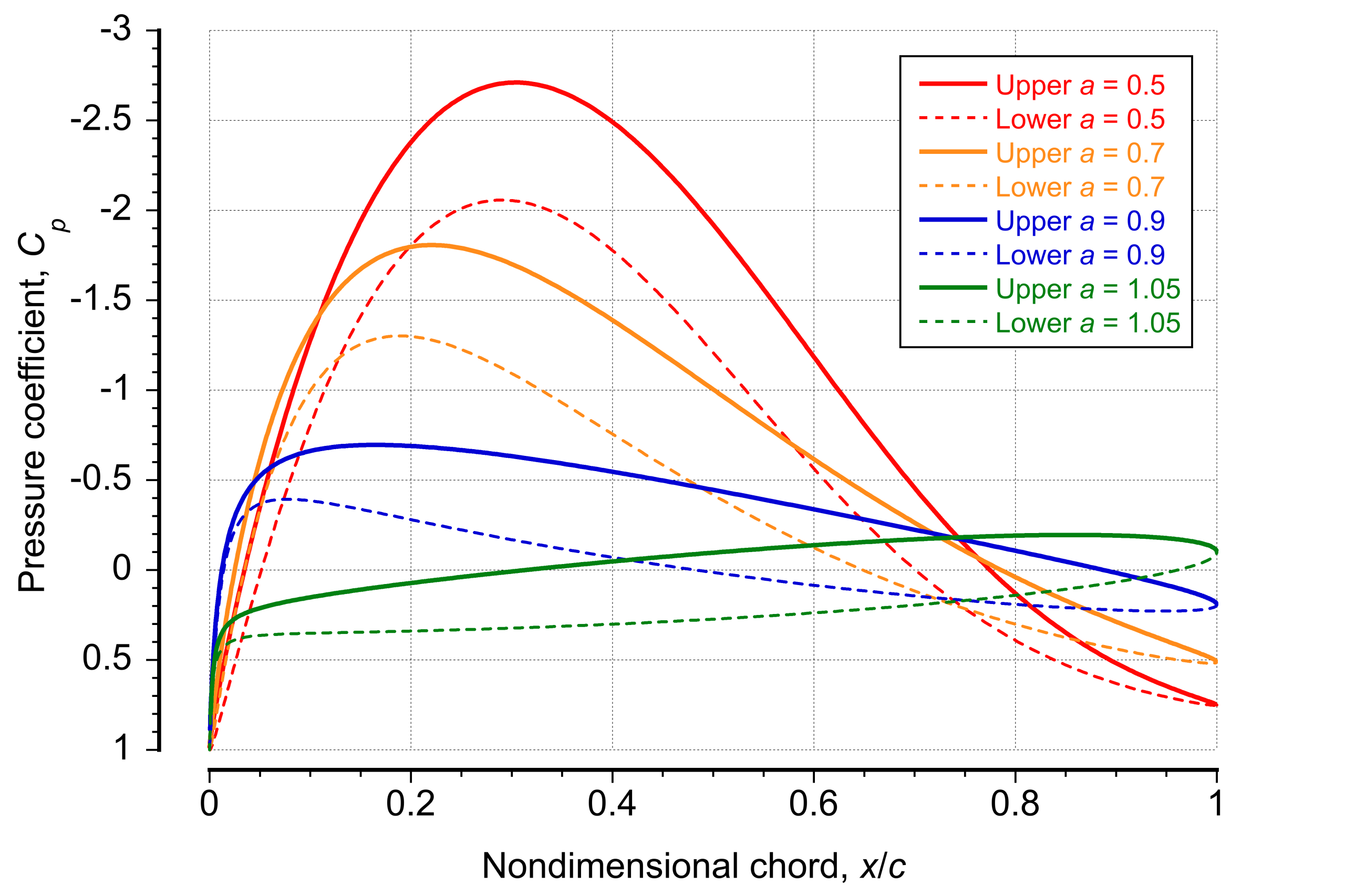 versus for a Joukowsky airfoil at zero angle of attack with offsets and .
Effects of Camber
The effects of camber on the airfoil pressure distribution are shown in the second figure below. Camber is a form of geometric curvature, and positive camber increases the effective angle of attack of the flow relative to the chord line. Camber also alters the pressure distribution along the chord. Even small increases in camber reduce the adverse pressure gradient on the upper surface near the trailing edge. This is an essential effect because a milder adverse pressure gradient helps to keep the flow attached to the airfoil at higher angles of attack. In this regard, camber plays a significant role, as cambered airfoils typically exhibit better aerodynamic performance than symmetric ones. Camber also softens the pressure gradient on the lower surface, which becomes more gradual with increasing camber. Although the lower surface contributes relatively little to the overall aerodynamic characteristics and boundary layer development, a milder gradient there delays the growth of the boundary layer. It thus helps reduce the pressure (form) drag on the airfoil section.
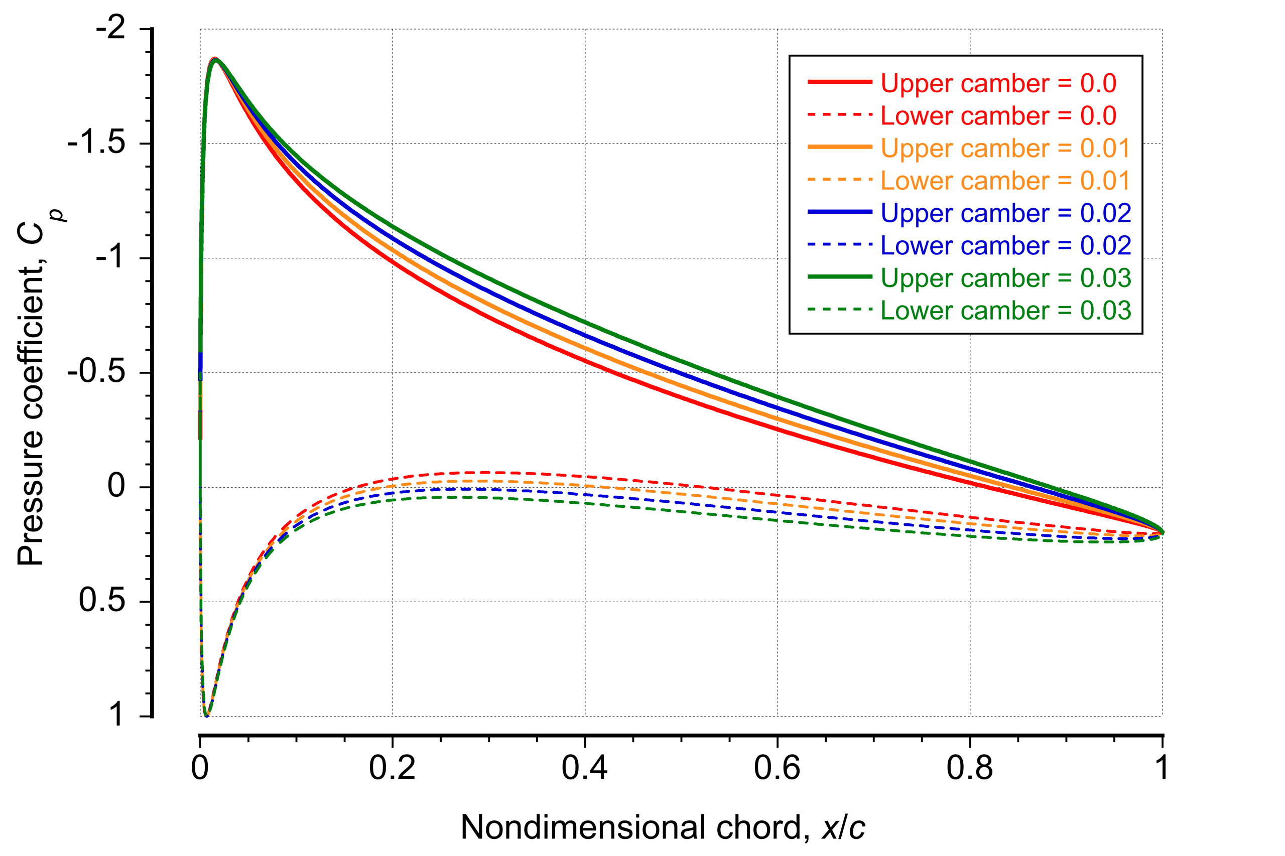 versus for a Joukowsky airfoil at an angle of attack of 5
 with offsets and .
Trailing-Edge Pressure Coefficient
At the trailing-edge cusp of a conformal-mapped Joukowsky airfoil, the theoretical value of the pressure coefficient is set by the Kutta condition, which ensures that the flow leaves the trailing edge smoothly with a finite velocity and so without a pressure jump. In this case, the trailing edge is not a stagnation point, i.e.,  . Recall that the Joukowsky mapping is defined as
(37) 
The cusp occurs at the trailing edge where  , which gives
(38) 
The flow velocity in the physical -plane is
(39) 
At the trailing edge,  , so to avoid a singularity in
  , the Kutta condition requires
(40) 
The determination of the circulation for a given airfoil shape and angle of attack ensures that the flow velocity is finite and leaves the trailing edge smoothly. Accordingly, the pressure coefficient at the trailing edge is given by
(41) 
For a symmetric Joukowsky airfoil at zero angle of attack, the velocity at the trailing edge is  , leading to
(42) 
However, in general, for cambered airfoils or at a nonzero angle of attack, the trailing-edge velocity is still finite. Still, it may differ in magnitude from , so  is not necessarily zero, but remains finite and is smooth in value as the trailing edge is approached. The essential condition is that there can be no pressure discontinuity across a cusped trailing edge, i.e.,
(43) 
a result that is apparent in the foregoing plots of the pressure distributions.
Lift & Pitching Moment
The determination of the lift and pitching moment coefficients is fundamental, as they describe the aerodynamic forces and moments acting on the airfoil and form the basis for performance analysis and design. The Kutta-Joukowski theorem has already been explained for determining lift; however, lift can also be obtained by integrating the pressure around the airfoil surface. Recall that in potential flow, a body will produce no drag, so this component need not be considered.
Lift Coefficient
The sectional lift per unit span, , is the vertical component of the surface pressure integrated around the perimeter of the airfoil, which can be expressed as
(44) 
where
(45) 
Substituting for gives
(46) 
and so
(47) 
The first integral vanishes by symmetry, leaving
(48) 
Writing
(49) 
means that  so only the cross‐term contributes, and consequently
(50) 
and hence
(51) 
which for small angles reduces to the classical Kutta-Joukowsky result that  . Because in the transformed plane, the chord is
(52) 
the corresponding lift coefficient is
(53) 
The theoretical result that  is much used in airfoil analysis, where the factor
  is referred to as the lift curve slope, i.e.,
(54) 
Moment Coefficient
The pitching moment on the airfoil can now be determined. The camber of the Joukowsky airfoil is described by in the -plane, where
(55) 
Integrating the moment of pressure about the quarter-chord gives
(56) ![\begin{equation*} M'_{c/4} = -\int_{0}^{2\pi} \Bigl(\tfrac12\,\varrho\,U^2\,C_p(\theta)\Bigr) \Re \Bigl\{\bigl[z(\theta)-z_{c/4}\bigr]\;i\,\frac{dz}{d\theta}\Bigr\} \,d\theta = -\,\pi\,\varrho\,U^2\,a\,\eta_0 \end{equation*}](https://eaglepubs.erau.edu/app/uploads/quicklatex/quicklatex.com-ef74580c75ec3e98c4f77a38ac1ec6a7_l3.svg "Rendered by QuickLaTeX.com")
and so the corresponding moment coefficient is
(57) 
where
(58) 
If required, using the application of statics, the moment about the leading edge is
(59) 
and so
(60) 
In terms of the coefficient, then
(61) 
Outcomes from Joukowsky Airfoil Analysis
In summary, the lift and moment coefficients for the Joukowsky airfoil are
(62) ![\begin{eqnarray*} C_l & = & 2\pi\,(\alpha - \alpha_{0}) \\[8pt] C_{m_{c/4}} & = & -\frac{\pi\,\eta_0}{2\,a} = -\frac{\pi\,\eta_0}{c} \\[8pt] C_{m,\mathrm{LE}} & = & -\frac{\pi\,\eta_0}{2\,a} + \dfrac{1}{2}\,C_l\,\cos \bigl(\alpha - \alpha_0\bigr) \approx -\frac{\pi\,\eta_0}{c} + \dfrac{1}{2}\,C_l \end{eqnarray*}](https://eaglepubs.erau.edu/app/uploads/quicklatex/quicklatex.com-3176dc4cbc175a56221fcc983b094aeb_l3.svg "Rendered by QuickLaTeX.com")
Notice that the aerodynamic center is defined as the point on the airfoil about which the moment coefficient is independent of the angle of attack . From the Joukowsky airfoil analysis, it can be seen that  is a constant because it depends only on the geometric offset and the circle radius , but not on the angle of attack . Therefore,
(63) 
By definition, the aerodynamic center is the point on the chord where the moment coefficient is independent of . Because this condition is satisfied at the 1/4-chord, it can be concluded that the aerodynamic center is located at
(64) 
Representative results for the lift coefficient versus angle of attack and the pitching moment about the quarter-chord versus angle of attack are shown in the figure below. The results are given for an airfoil with and without camber. The symmetric (uncambered) airfoil produces a theoretically derived lift curve slope of per radian, and the lift coefficient is zero at zero angle of attack. The theoretical predictions agree well with measurements up to an angle of attack of about  , beyond which the airfoil begins to stall, and the theory no longer applies.
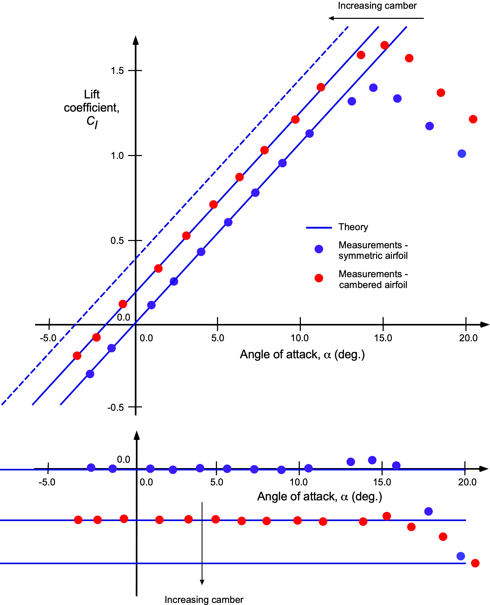
The introduction of camber shifts the lift curve to the left, although the slope of the curve remains close to per radian. Consequently, the zero-lift angle of attack becomes negative, which is typically on the order of  to
to  for practical airfoils. While camber increases the maximum lift coefficient of the airfoil, it does not substantially alter the angle of attack at which stall occurs. Generally, camber increases the drag of an airfoil, something that is not predicted by the potential flow theory, so that practical airfoils will incorporate minimal camber.
The corresponding pitching moment about the 1/4-chord is nearly zero for the symmetric airfoil because the 1/4-chord lies close to the aerodynamic center. In theory, the aerodynamic center is located at the 1/4-chord point. For a cambered airfoil, the pitching moment curve is shifted to increasingly negative values. In this case, the aerodynamic center remains near the quarter-chord, as evidenced by the constant slope of the moment curve versus angle of attack. However, camber introduces a nose-down moment offset that increases with the degree of camber.
Kármán-Trefftz Airfoils
The Kármán-Trefftz airfoil transformation is a generalization of the classical Joukowsky transformation. It belongs to a broader class of conformal mappings used to construct analytic solutions for the flow over airfoils. Again, the goal of such mappings is to convert the known solution of potential flow around a circular cylinder into the flow around a more realistic airfoil shape using an angle-preserving transformation between two complex planes.
The Kármán-Trefftz mapping enables the generation of airfoils with a finite trailing-edge angle, which is representative of most practical airfoil shapes. This feature is absent in the original Joukowsky airfoil, which ends in a cusp. This goal is achieved by modifying the mapping function such that the behavior at the trailing edge becomes algebraically singular only to the degree needed to generate a wedge rather than a cusp.
The transformation is written as
(65) 
or more generally as
(66) 
where and are complex coordinates in the airfoil and circle planes, respectively. The coefficient  is a real constant that defines the location of the two branch points
  , and
, and  is a real exponent strictly greater than 1 that determines the angle of the trailing edge.
To understand this, consider the behavior of the mapping function near the branch point  , which will correspond to the trailing edge of the airfoil. Let
(67) 
Near this point, the numerator and denominator of the transformation behave like
(68) 
Substituting into the mapping and expanding in powers of  , then
(69) 
where  is the trailing-edge point, and the singularity is governed by the exponent
  . The angle between the upper and lower surfaces at the trailing edge is then
(70) 
Therefore, when  , the Joukowsky case is recovered with
  , a cusp. When
  , the trailing edge opens up to produce a finite angle. An example of a symmetric Kármán-Trefftz is shown in the figure below.
To proceed from the geometric transformation to the flow solution, the potential flow in the -plane can be determined. Around a circle of radius , centered at  , the complex potential for a uniform flow at angle and circulation is given by
(71) 
Differentiating this gives the complex velocity field in the -plane, i.e.,
(72) 
To obtain the physical velocity in the airfoil plane, differentiating the Kármán-Trefftz transformation gives
(73) 
The velocity in the -plane is then
(74) 
The Kutta condition requires that the flow leave the trailing edge smoothly, i.e., with finite and equal velocity from above and below. This condition removes the singularity at and fixes the value of the circulation. To enforce it requires
(75) 
Substituting into the velocity expression gives
(76) 
Solving for gives
(77) 
as before, from which the lift follows as for the Joukowsky airfoils.
It should be noted that the practical application of the Kármán-Trefftz transformation requires either careful parameter selection or numerical iteration to accurately match target airfoil shapes. Today, with the advent of numerous other numerical methods for predicting airfoil flows, the Kármán-Trefftz method is of historical interest rather than practical significance. Nevertheless, as with the Joukowsky transformation, it can provide flow solutions about airfoil shapes that can be used as check cases or validation against other methods.
Other Conformal Mapping Methods
While the Joukowsky and Kármán-Trefftz transformations offer closed-form solutions with interpretability and reasonable geometric fidelity, other, more general conformal mapping approaches have also been proposed. Among them are Theodorsen and Garrick’s complex series expansions and the Schwarz-Christoffel transformation, both of which offer greater mathematical flexibility but at the expense of much greater computational effort.
Theodorsen and Garrick’s Method
Theodore Theodorsen and Theodorsen and Garrick[9] introduced a generalized mapping[10]of the form
(78) 
where  is the complex coordinate in the physical (airfoil) plane,
  is the complex conjugate of , is the corresponding point in the transformed (circular) plane, and
  and
and  are complex-valued coefficients that encode the camber and thickness of the airfoil.
The objective is to map an arbitrary airfoil shape to a near-circle in an auxiliary -plane, allowing for the application of classical potential flow solutions. This goal is achieved through a combination of complex-variable transformation, radial fitting, and coefficient identification. The procedure consists of the following steps.
- Given a set of Cartesian coordinates
 , the complex representation of the airfoil contour can be defined as
(79)

The points
 should describe a closed, ordered loop around the airfoil, including both upper and lower surfaces.
 - To simplify the mapping, the airfoil is translated so that its centroid lies at the origin. The complex centroid is computed using
(80)

and each point is translated accordingly using
(81)

This step ensures the airfoil geometry is centered for radial fitting.
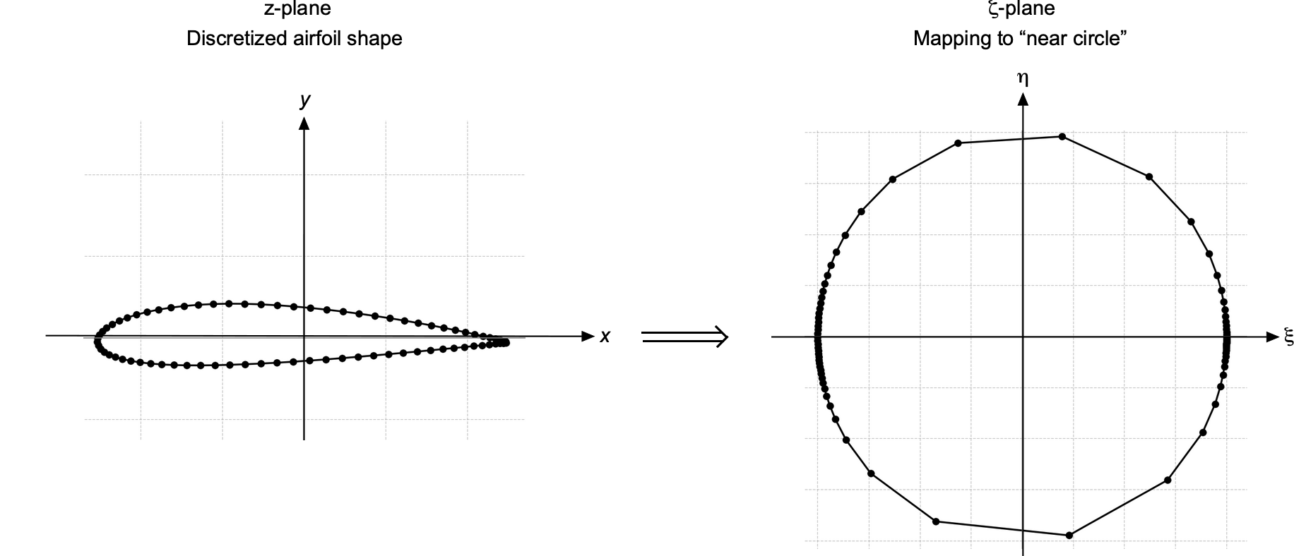
- One may then numerically invert the Joukowsky transformation to obtain the image of the airfoil in the -plane as a near-circle. For each centered point , it is necessary to compute
(82)

which will lie close to the unit circle. The appropriate branch of the square root is selected to ensure continuity. The resulting image, as shown in the figure below, is referred to as the “near circle” and serves as the target domain for the inverse mapping.
Inverse mapping of the airfoil to an approximate “near circle.” - Each is also converted to polar coordinates, i.e.,
(83)

The angles
 are unwrapped and sorted in increasing order to span a full range of
 ![[-\pi, \pi]](https://eaglepubs.erau.edu/app/uploads/quicklatex/quicklatex.com-bf37d6fc4e110827e1d3996863dba806_l3.svg "Rendered by QuickLaTeX.com") or
or ![[0, 2\pi]](https://eaglepubs.erau.edu/app/uploads/quicklatex/quicklatex.com-427a9e5eb925adb1c9ebc6a1f9d51656_l3.svg "Rendered by QuickLaTeX.com") , ensuring a consistent representation around the airfoil. A periodic cubic spline is fitted to the sorted pairs
, ensuring a consistent representation around the airfoil. A periodic cubic spline is fitted to the sorted pairs  to obtain a smooth function of the form
(84)

This function represents the airfoil as a radial shape, as shown in the figure below. One may then define a regularized mapping to the
-plane as(85)

which yields a smooth closed curve in the
-plane.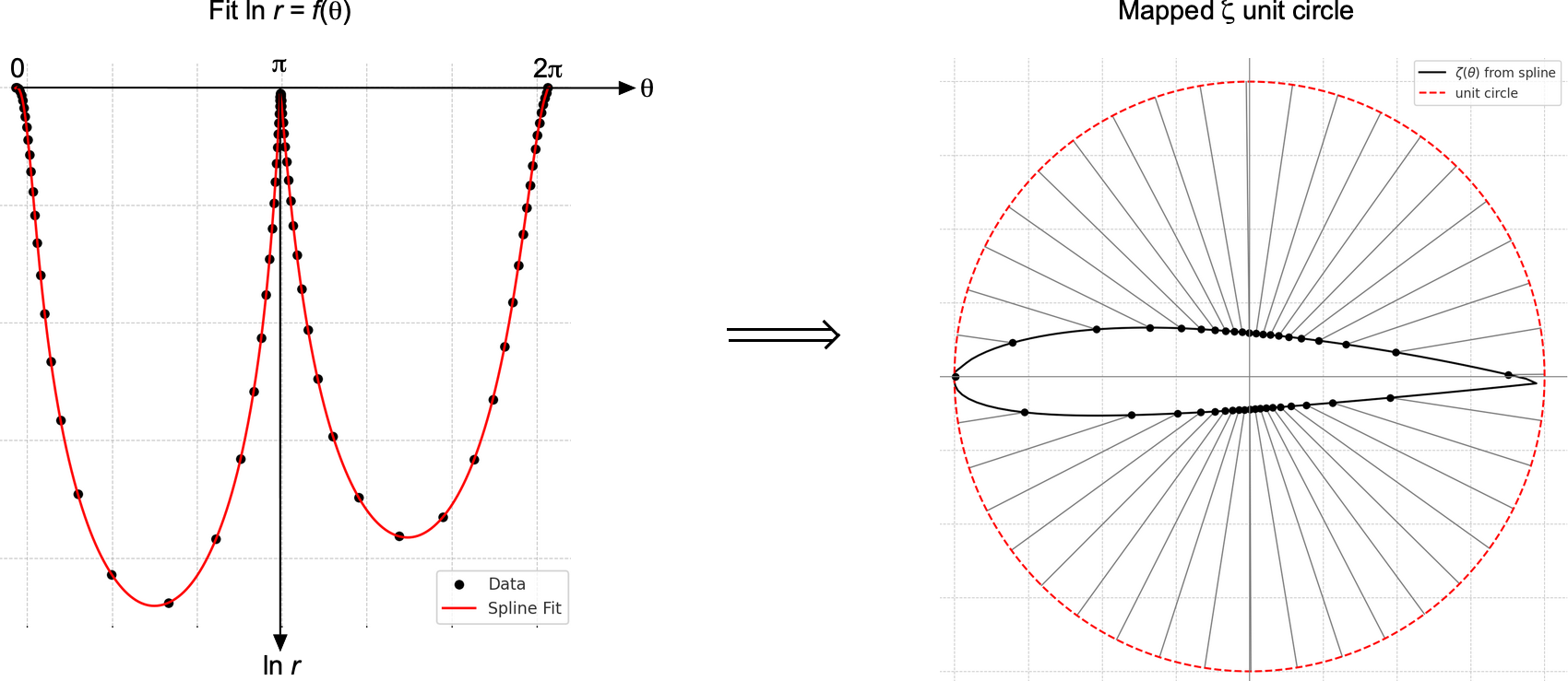
Unwrapping the airfoil and expressing its shape in polar coordinates allows a curve fit to help map to the unit circle. - At this point, a set of corresponding points
 is available relating the physical airfoil to the near-circle. The Theodorsen-Garrick inverse mapping is then fitted using
(86)

where the coefficients
 and
and  are determined by solving a least-squares problem using the known
  pairs.
The velocity field and pressure distribution are then derived from a potential flow solution in the -plane. These are then transformed back to the physical plane using the inverse of the mapping . To ensure a physically meaningful flow at the trailing edge, the mapping should satisfy the Kutta condition, which is enforced by adjusting the coefficients so that the trailing edge becomes a sharp cusp and the velocity remains finite.
This entire method, although lengthy and somewhat unwieldy, enables the analytical approximation of arbitrary airfoil shapes using classical conformal mapping theory. However, today this formulation is rarely used directly because, in practice, one must fit the coefficients to match a desired airfoil shape, which typically requires inverse mapping techniques or numerical optimization. Additionally, low-order truncations with  10 often produce distorted or unphysical geometries, and high-order expansions introduce additional mathematical complexity without guaranteeing convergence or practical interpretability. The method is, therefore, of more pedagogical rather than practical value.
Schwarz-Christoffel Transformations
Hermann Schwarz and Elwin Christoffel independendly introduced polygonal types of conformal mappings, which have since become known as the Schwarz-Christoffel transformations[11] provides an even more general framework by mapping canonical domains such as the upper half-plane onto arbitrary polygonal regions in the physical plane. This method can create airfoils with sharp corners and finite-angle trailing edges, defined precisely through interior angles. However, the method is almost entirely numerical; the “parameter problem” must be solved to determine the prevertices of the transformation, and the mapping function must be evaluated numerically. These requirements make the Schwarz-Christoffel transformation analytically intractable and computationally intensive. While modern software packages can automate the process, the resulting shapes are generally polygonal approximations rather than smooth, aerodynamically realistic airfoils. Again, today, such methods remain important within the framework of classical airfoil theory, except perhaps for check cases, where other numerical methods have largely replaced them.
Thin Airfoil Assumption
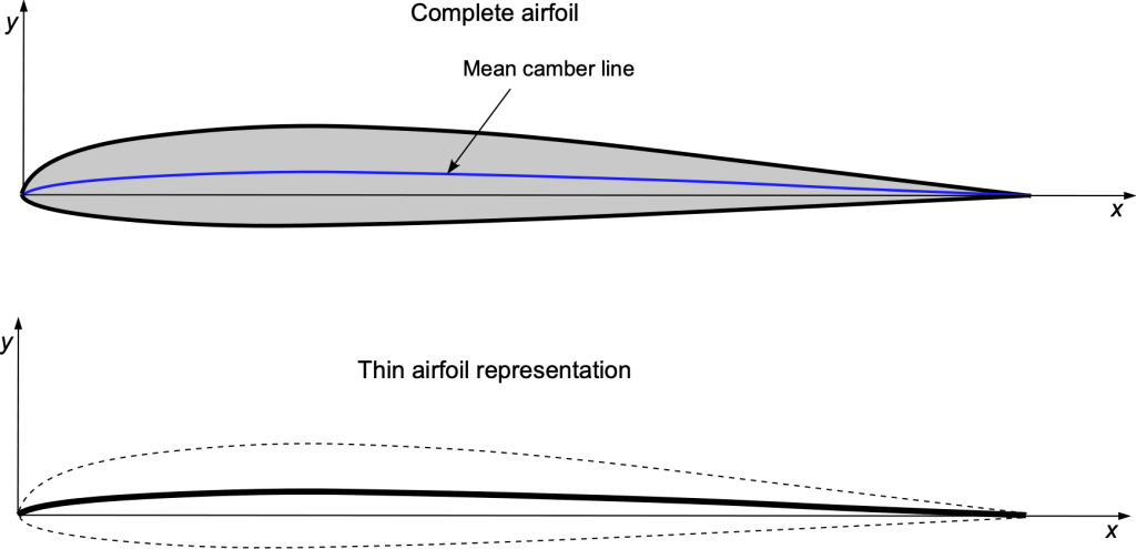
Many aerodynamic properties of airfoil sections with finite thickness can be closely approximated by an aerodynamic analysis about their mean camberline. The mean camberline is defined as the locus of points situated halfway between the upper and lower surfaces of the section measured normal (perpendicular) to the mean line, as shown in the figure below. Airfoils without camber are called symmetric airfoils, characterized by the same camber on both the upper and lower surfaces.
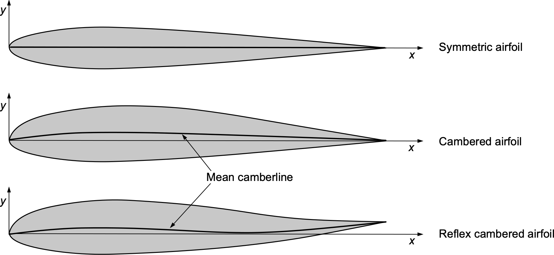
Using some camber, especially over the airfoil’s leading edge, improves its aerodynamic characteristics, particularly at higher angles of attack, such as increasing the maximum lift coefficient. However, this useful capability is usually accompanied by increased pitching moments, which may be undesirable. In this regard, reflex camber, a form of upward camber at the trailing edge, provides many of the aerodynamic benefits of positive camber over the nose region of the airfoil but with reduced pitching moments.
In the thin airfoil theory, the camberline itself becomes the airfoil shape on which to perform the aerodynamic analysis, as shown in the figure below. In other words, the aerodynamic effects of thickness are removed and ignored aerodynamically. Indeed, while the thickness distribution affects the pressure distribution around the airfoil, the effects are symmetrically disposed between the upper and lower surfaces. So, to first order, they cancel each other out in their effects on the integrated properties, such as lift and pitching moment.
The prominent aerodynamic properties that are primarily associated with the shape of the camberline include:
- The chordwise loading distribution, i.e., the velocity and pressure distributions across the chord.
- The magnitude of the lift coefficient, , and the slope of the lift curve, i.e., the lift curve slope,
 .
. - The angle of attack for zero-lift, , i.e., the angle to which a cambered airfoil must be depressed to generate no lift.
- The pitching-moment coefficient about some convenient reference axis, such as 1/4 chord, i.e.,
 .
. - Location of the center of pressure,
 , and aerodynamic center,
  .
.
Theory of Vortex Sheets
The theory of vortex sheets is fundamental in aerodynamics, particularly in thin-airfoil theory and surface-singularity or “panel” methods. It provides a mathematical framework for modeling the flow velocity and pressure distribution around an airfoil and predicting its aerodynamic performance. The figure below illustrates a vortex sheet. 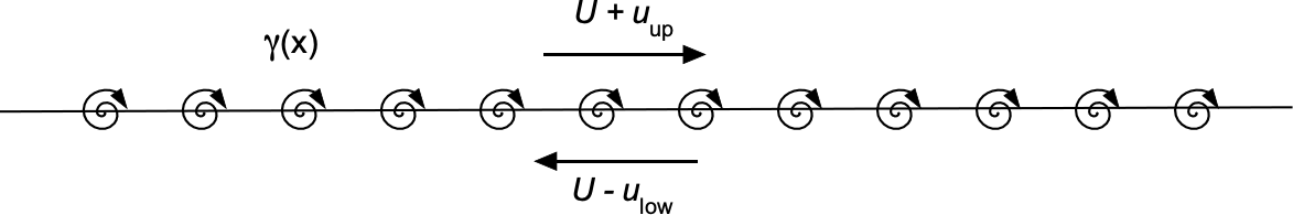
A vortex sheet singularity has a jump in velocity and pressure over its surface. The vortex sheet strength,  , which can vary along the length of the sheet, represents the jump in tangential velocity across the sheet, i.e.,
(87) 
The jump in tangential velocity also leads to a pressure jump,  , i.e.,
(88) 
where  is the average velocity. Integrating this pressure jump across the sheet generates a lifting force given by
(89) 
Alternatively, because the total circulation is given by
(90) 
Then, using the Kutta-Joukowski theorem, the lift is given by
(91) 
Thin Airfoil Theory
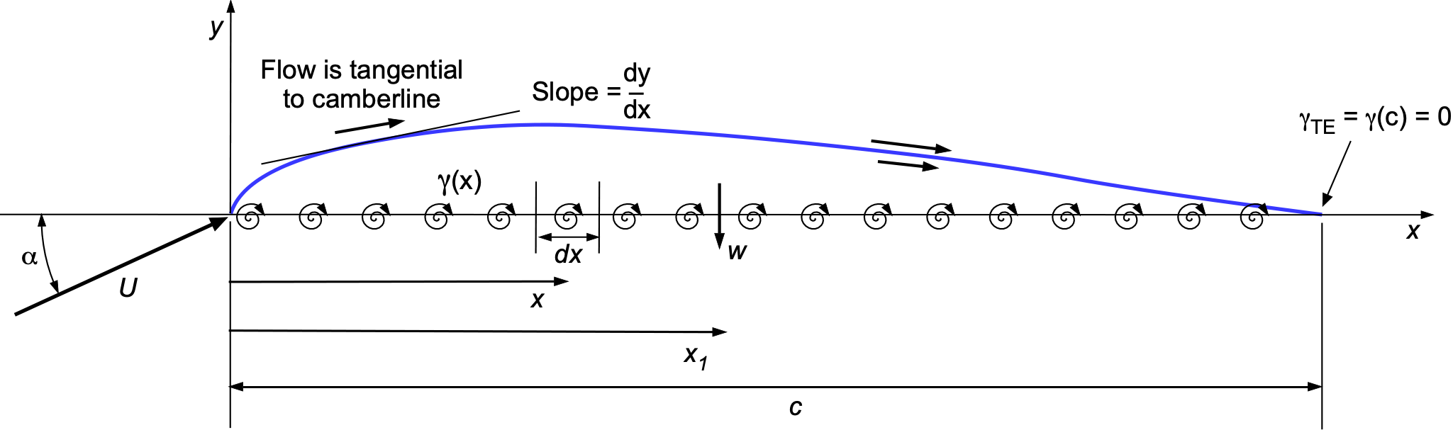
With the groundwork now done, the thin-airfoil theory can be presented. Vortex sheets play a crucial role in modeling the flow around an airfoil. The present treatment follows Glauert’s approach. The key idea is to represent the flow over the airfoil by placing a vortex sheet of unknown strength along the camberline, as illustrated in the figure below. Because the camber is assumed to be small, the problem can then be linearized without much loss of accuracy by placing the vortex sheet along the chord line. Then, the approach is to calculate the vortex sheet strength along the chord line, ensuring that the flow is tangential to the camber line, i.e., satisfying the no-penetration condition. In addition, the Kutta condition, which is an empirical observation, must be satisfied, in that the flow must leave the trailing edge smoothly.
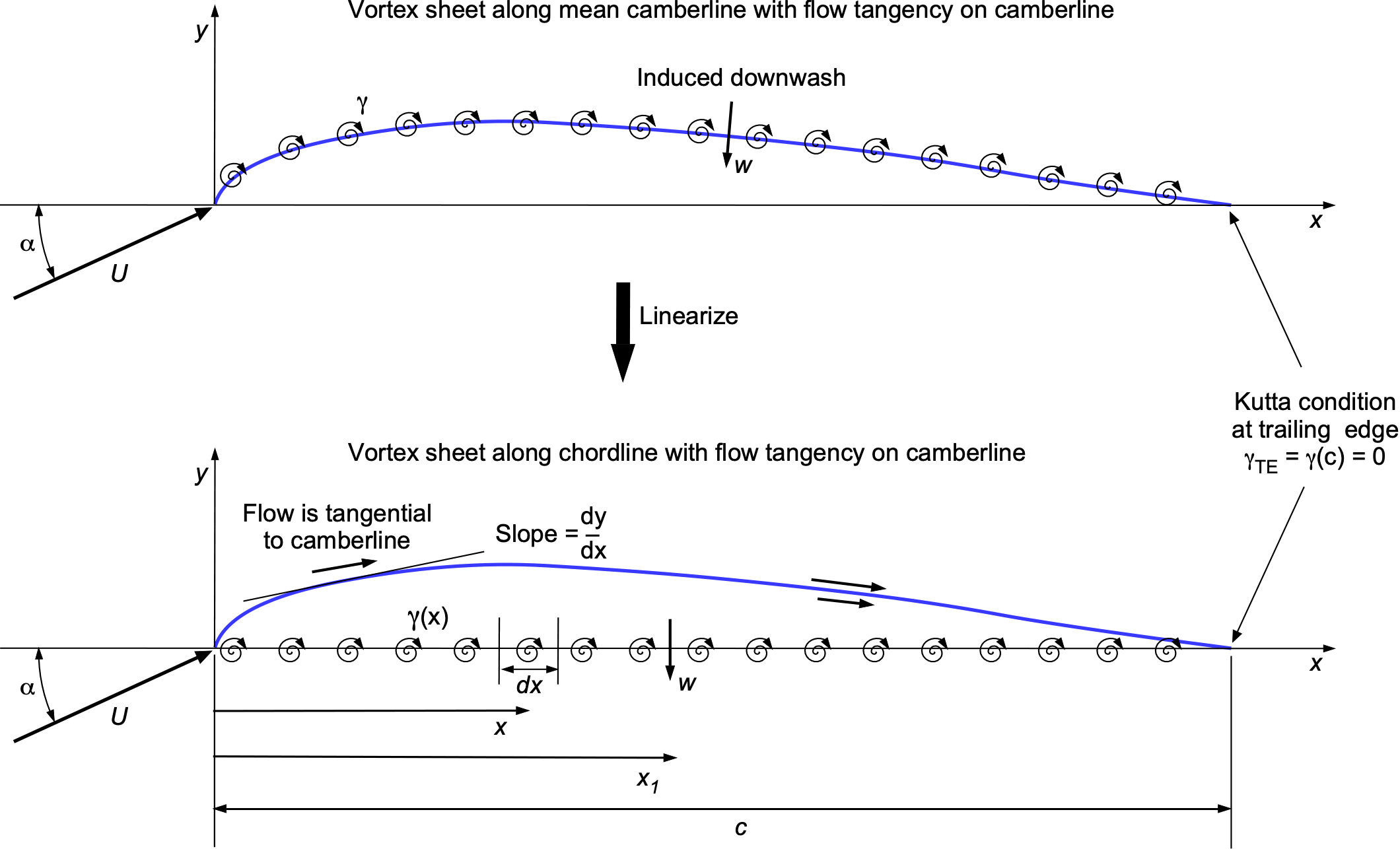
The strength of the sheet,  , is partially determined using the tangential flow (no-penetration) boundary condition, i.e., it will be apparent from the figure below that
(92) 
and so to a small angle assumption
(93) 
This latter equation is a formal statement of the no-penetration or flow tangency requirement on the camberline.

The auxiliary boundary condition is at the trailing edge, where the vortex sheet strength must go to zero to satisfy the Kutta condition, i.e., there is a smooth flow with no jump in velocity, which means that
(94) 
If the sheet strength is then suitably determined according to these boundary conditions, the total circulation around the airfoil section, , is
(95) 
This leads to the pressure distribution over the vortex sheet and the integrated quantities on the airfoil, such as lift, per the Kutta-Joukowski theorem, i.e.,
(96)
Now, more carefully consider the downwash velocity caused by an element of the vortex sheet, as shown in the figure below. Using the Biot-Savart law, the downwash,  , at a point
  caused by an element at
  will be
(97) 
Therefore, the total downwash from the sheet at any point is
(98) 
Recall that the boundary condition for flow tangency is
(99)
which leads to
(100) 
This latter equation is called the fundamental or governing equation of thin airfoil theory. Again, the sheet strength is unknown, which must now be solved subject to the boundary conditions of flow tangency on the camberline as well as the Kutta condition at the trailing edge.
The Kutta condition, which forms the second boundary condition after flow tangency on the camberline, is expressed as
(101) 
 and
and  are the tangential velocities on the upper and lower surfaces, respectively, as shown in the figure below. Three types of trailing edges are encountered in practical airfoils: a convex trailing edge, a trailing edge with a finite enclosed angle, and a trailing edge that forms a cusp.
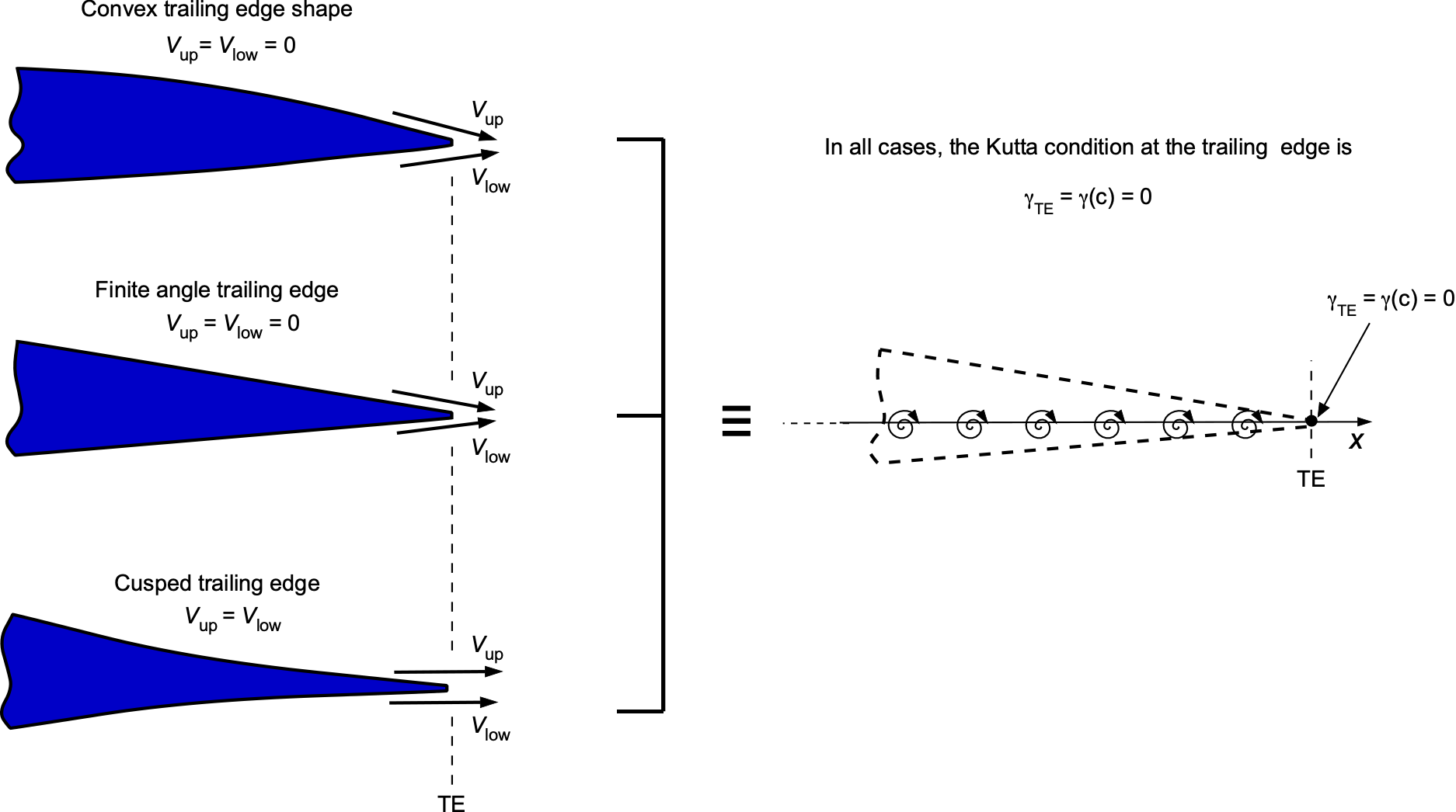
A rounded trailing edge with finite curvature characterizes a convex trailing edge. Here, the tangential velocities and must have the same finite value as the flow leaves the trailing edge, so the only solution is that  , i.e., a stagnation point where = 1. Therefore,
  . For a finite-angle trailing edge, the upper and lower surfaces meet at a sharp point with a nonzero included angle. Again, the tangential velocities and must have the same finite value as the flow leaves the trailing edge, so the only solution is that , i.e., a stagnation point and = 1. Therefore, , as before.
A cusped trailing edge is characterized by the upper and lower surfaces meeting tangentially at an infinitely sharp point. In this case,  , but it is not a stagnation point and so is not necessarily equal to 1. Nevertheless, the theory of vortex sheets again ensures that . In all cases, the Kutta condition ensures smooth, physically consistent flow at the airfoil’s trailing edge, enabling accurate lift predictions and overall aerodynamic performance.
Conformal Mapping & Thin Airfoil Theory
A primary difference between the conformal mapping method and thin airfoil theory is that conformal mapping enables the calculation of the entire flow field and streamlines. In contrast, thin airfoil theory focuses solely on the integrated forces and moments. When the airfoil is very thin, gently curved, and set at a modest angle of attack, these three departures from a flat plate, thickness, camber, and angle are all comparably small. Therefore, they can be represented by a single small parameter and treated together in the analysis.
Recall that the Joukowsky transformation is
(102) 
with , which maps the circle to an airfoil of chord  . To derive the thin airfoil limit, introduce a single small parameter
  , and let the generating circle in the conformal mapping differ only
  from this reference shape, i.e.,
(103) 
so the thickness parameter  , camber offset , and the angle of attack are all . Substituting Eq. 103 into Eq. 102 and retaining the first non-vanishing terms gives the airfoil surface as
(104) 
(105) 
Here, the function  represents the geometric deviation from a flat plate as a result of both camber and thickness. Because this deviation is small, the impermeability condition can be linearized on the flat reference line
  . Letting
  be the first-order perturbation potential, the linearized boundary condition becomes
(106) 
where  is the effective angle of attack, also of . This form reflects that the normal component of freestream velocity,
  , must be canceled by the surface-normal velocity induced by the vortex sheet, corrected for the slope of the surface,
  . The flow fields for both the flat-plate and cambered-plate solutions are shown below.
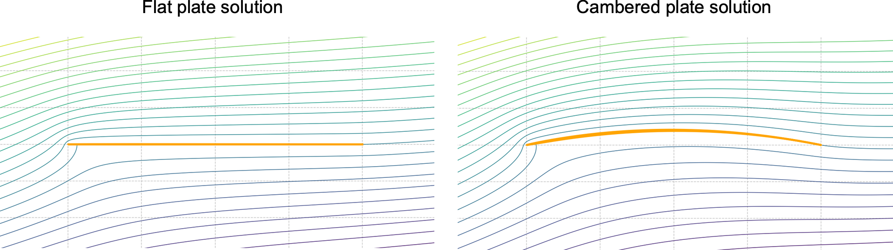
At this order, the exact mapping is no longer necessary if only the integrated aerodynamic values are required. The same surface velocity distribution is obtained by placing a bound vortex sheet along the reference line . Using the Biot-Savart law to compute the induced normal velocity and equating it to Eq. 106 produces the thin-airfoil singular integral equation given by
(107) 
The finite-velocity requirement at the sharp trailing edge reduces, in this linearized situation, to the Kutta condition  . The foregoing are precisely the thin-airfoil modeling assumptions: a flat reference line, a linearized boundary condition, a Kutta condition at the trailing edge, and a bound vortex sheet whose strength is the unknown, which is obtained directly as the limit of the exact conformal-mapping solution.
Fourier Representation of Vortex Sheet Strength
Returning to the thin airfoil problem, the significance of the foregoing concepts can be understood and appreciated. While Munk did not take the thin airfoil theory to a practical conclusion, Glauert realized that it had to be expressed in a form that could be readily solved to be of practical help. To this end, Glauert was to follow the work of Bairnbaum[12]to use a Fourier series representation of vortex sheet strength to simplify the mathematical treatment of predicting the distribution of aerodynamic loads along an airfoil. Using a Fourier series provided an elegant and systematic way to solve the fundamental equation of thin airfoil theory.
This approach has several advantages. First, using a Fourier series to represent the vortex sheet strength reduces the integral equation into a set of algebraic equations, making it easier to solve. Second, the Fourier series expansion decomposes the vortex sheet strength into independent modes, which can be combined using the principle of superposition. By expressing the loading as a sum of sine modes, the analysis becomes more straightforward because trigonometric functions are well understood. Each mode corresponds to specific aerodynamic effects, such as overall lift or chordwise loading variations. Finally, the Fourier series coefficients can be assigned direct physical interpretations, as will be shown.
Glauert Transformation
To solve the thin airfoil problem in a very general way, Glauert first used a linear to polar coordinate transformation as given by
(108) 
where each point on the chord is mapped to an equivalent  value, as shown in the figure below. This transformation was also used in the development of the lifting-line theory.
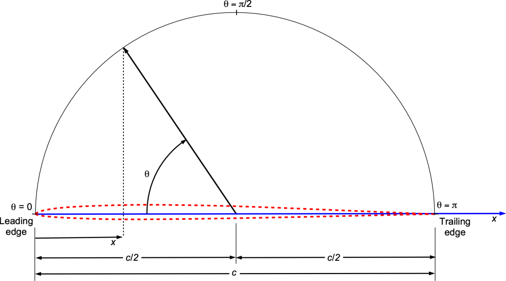 to an angular coordinate in .
In terms of the coordinate, the fundamental or governing equation of thin airfoil theory is now
(109) 
where maps to and maps to  . The solution for the vortex strength
  is then expressed as
(110) 
where  depends only on , and depends on the shape of the mean camberline.
Fourier Loading Modes
Notice that the primary loading term, , is given by
(111) 
the shape of which is shown in the figure below in terms of the coordinate and the coordinate.
 Fourier loading mode mimics the chordwise differential pressure on a subsonic airfoil.
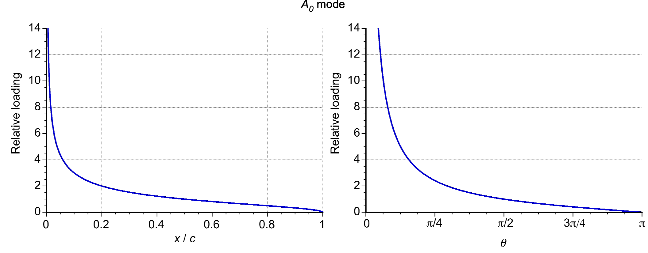
The term is significant because it mimics the angle-of-attack loading on a low-speed airfoil, as illustrated in the figure below. However, the leading edge singularity of the function should be noted as  . In thin airfoil theory, the pressure coefficient difference between the upper and lower surfaces,
  , is given by
(112) 
in accordance with the principles of vortex sheets. This pressure loading can also be written in terms of the coordinate as
(113) 
where  and is the angle of attack in radians. In practice, the leading-edge suction value is less than the theoretical maximum, which tends to infinity. This result has some significance in calculating the pressure drag, which is considered later in this chapter.
The  mode represents the first harmonic of the chordwise loading distribution, as shown in the figure below. It exhibits asymmetric variation that affects lift and pitching moment. The
  mode represents the second harmonic of the loading distribution. This mode is symmetric about the mid-chord and will not affect the lift, but it will affect the moments.
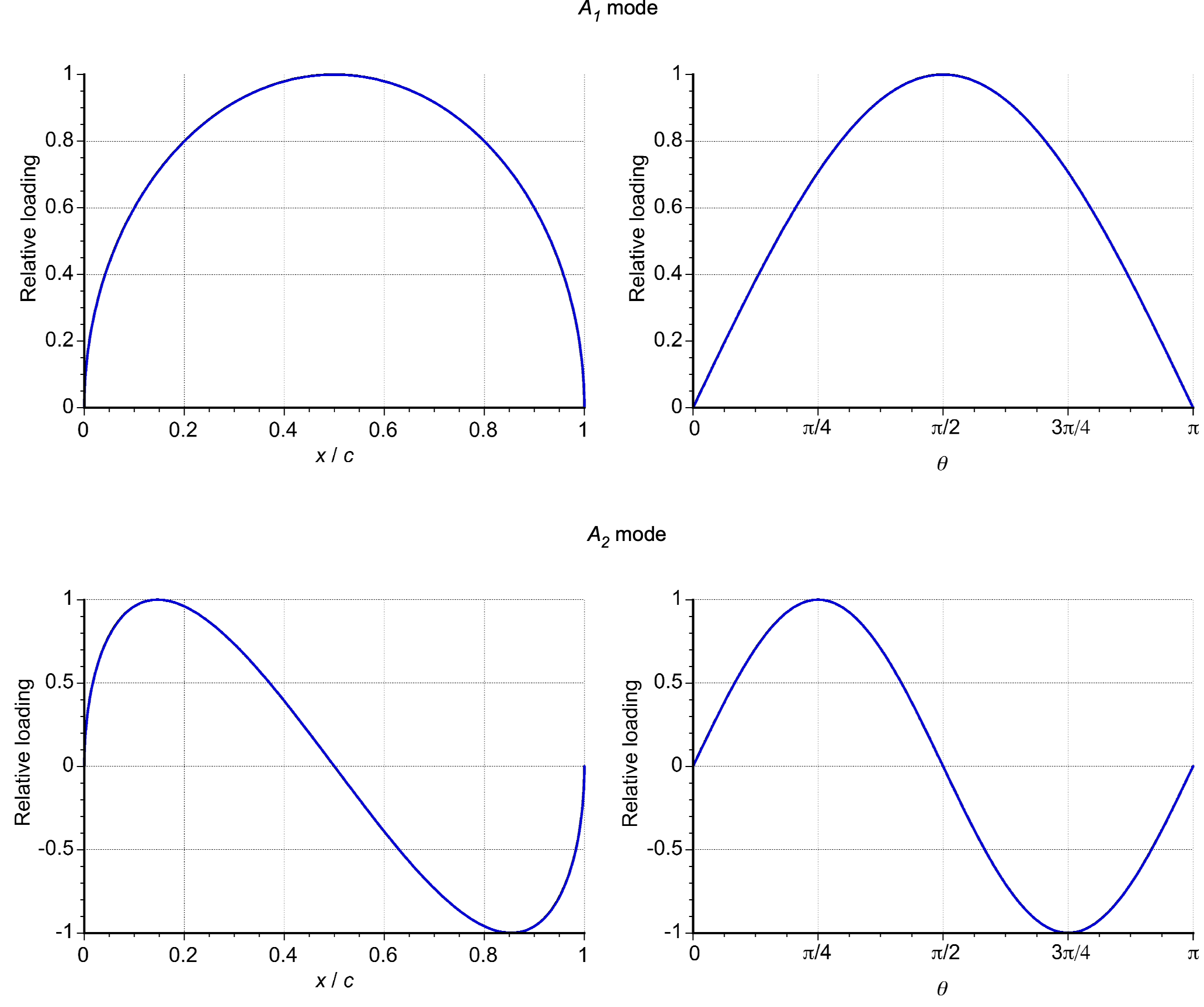 and modes will contribute to both the lift and the pitching moments.
The  ,
,  , and higher modes also have no symmetry about the mid-chord, indicating none of these modes will affect the lift or the pitching moments. This outcome will be apparent from an examination of the and modes, as shown in the figure below, where their integrals from
  to
to  are all zero. These modes, however, do affect the pressure distribution. If the prediction of the pressure distribution is a desired outcome, it must be calculated using a sufficiently high number of modes.
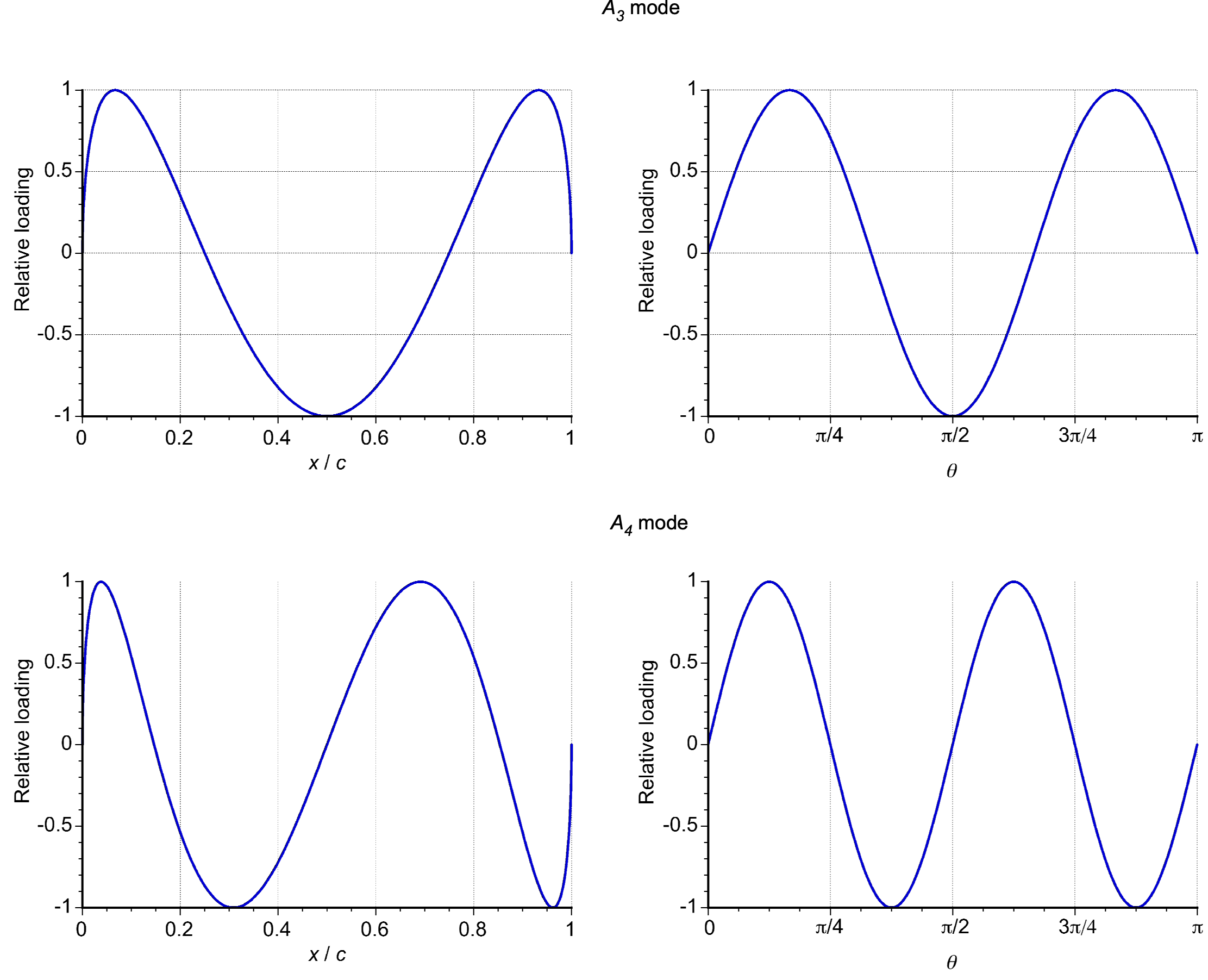 and higher modes do not affect the lift or the pitching moments.
Determining the Loading Coefficients
The primary loading coefficient is determined by evaluating
(114) 
where  is the slope of the camberine. If the camberline is known in terms of some simple polynomial or other easily differentiable function, then this integral can be evaluated analytically.
Likewise, the coefficients for  are determined using
(115) 
It will be noted that for a symmetric airfoil,  , then
  . However, for a cambered airfoil where
  , and the values must be calculated based on the specific camberline,
  .
.
Lift & Lift Coefficient
The lift per unit span, , is obtained by integrating the chordwise circulation distribution, , over the chord, i.e.,
(116) 
Because the circulation distribution is given using the Fourier series expansion
(117) 
Substituting this into the prior equation for the lift gives
(118) 
Separating the terms gives
(119) 
Evaluating the first term gives
(120) 
and the second term (for  ) is
) is
(121) 
It will be apparent that the higher-order terms ( ) do not contribute to the lift.
Therefore, after evaluating the integrals, then
(122) 
This shows that lift depends only on the first two modes, and  , because of the orthogonality of trigonometric functions.
The lift coefficient is defined conventionally as
(123) 
Substituting the result for gives
(124) 
and simplifying gives
(125) 
Notice that the lift-curve-slope is  per radian angle of attack, independent of camber. This result is obtained because
(126) 
The term is a constant for a given airfoil because it depends only on the camberline, not the angle of attack. Differentiating with respect to gives
(127) 
Therefore, the lift-curve slope is determined solely by the term, which includes the linear dependence on . The term affects the value of at a specific , but it does not affect the slope of the lift curve.
Comparison with Lift Measurements
One of the strengths of thin airfoil theory is its ability to accurately predict the linear relationship between the lift coefficient, , and angle of attack, , at small angles and for moderately cambered airfoils. For example, the relationship
(128) 
matches measured data well for thin airfoils with low thickness and fully attached flow, as shown in the figure below. It is particularly effective for explaining aerodynamic trends, such as the impact of camber on the zero-lift angle of attack, , and zero-lift pitching moment,  .
.
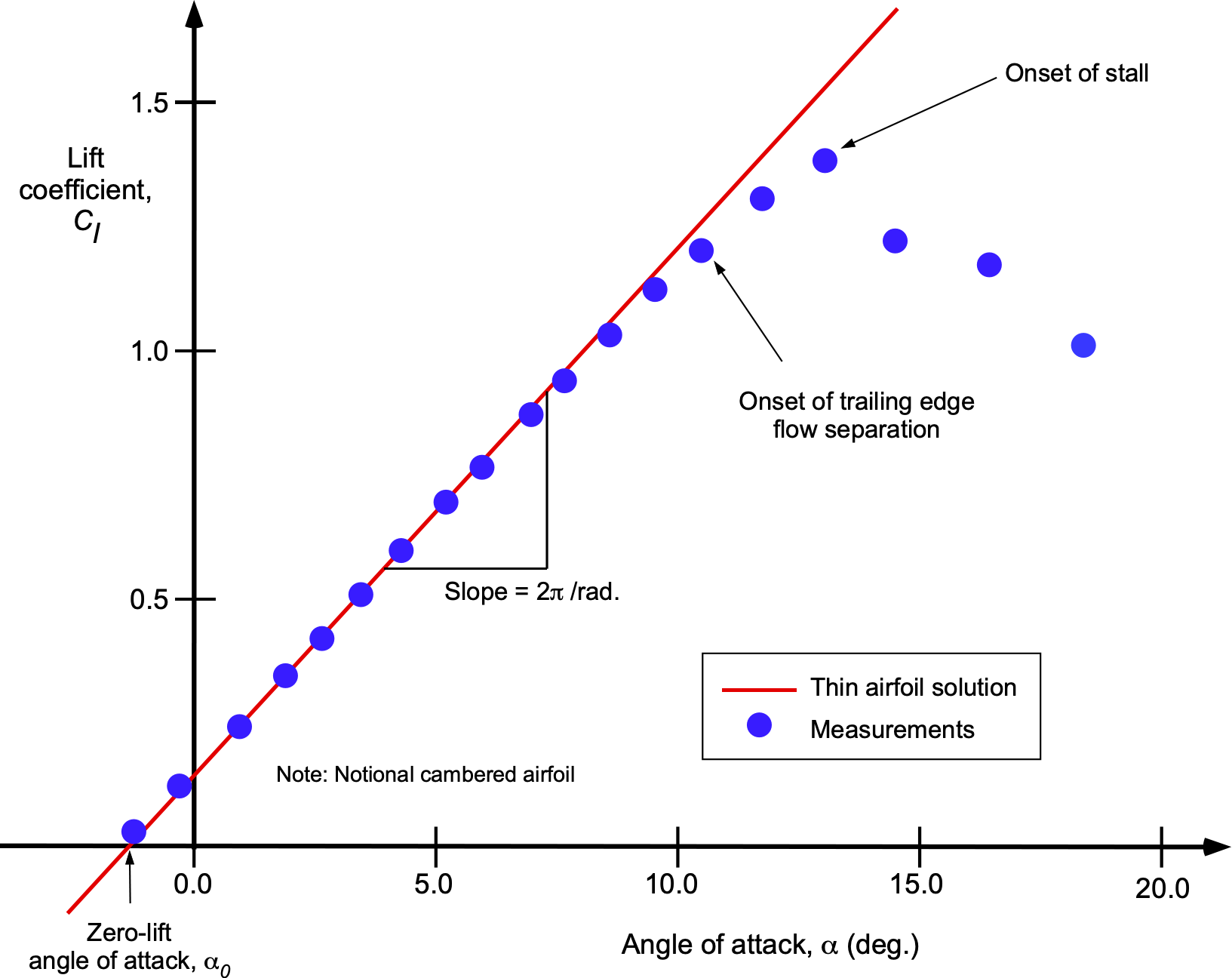
Compared with measured data, the thin airfoil theory accurately predicts a lift curve slope of per radian for thin, symmetric airfoils under subsonic conditions. However, measurements for most airfoils show slightly lower slopes because of thickness and viscous effects. The theory does not predict the sharp drop in lift near the stall because it cannot model flow separation. Overall, thin airfoil theory is most effective for thin, low-camber airfoils operating at low to moderate angles of attack and in subsonic flow.
One of its primary assumptions is that the airfoil has zero thickness, which means it cannot account for the effects of finite thickness, such as increased drag, boundary layer separation, or compressibility at high speeds. It also assumes a fully attached flow, which makes it invalid near stall or at high angles of attack where flow separation occurs. Furthermore, because it ignores viscosity, the theory cannot predict drag or account for Reynolds number effects, especially at Reynolds numbers below 10 . At higher angles of attack, for airfoils with significant camber, and at higher flow speeds where compressibility effects become important, the linear assumptions of the theory break down, leading to substantial deviations from measurements.
Pitching Moments
The expression for the pitching moment per unit span about the leading edge is given by
(129) 
Using the chordwise loading distribution, the pitching moment becomes
(130) 
Using the trigonometric simplification
(131) 
Performing the integration loads to
(132) 
and
(133) 
and
(134) 
Notice that higher-order terms ( ) vanish because of the orthogonality of trigonometric functions.
The final expression for the pitching moment about the leading edge is
(135) 
and the pitching moment coefficient about the leading edge is then
(136) 
Aerodynamic Center
The aerodynamic center ( ) is the point along the chord of the airfoil where the pitching moment coefficient,
  , is constant and does not change with the angle of attack, . For all thin airfoils, including both symmetric and cambered airfoils, the aerodynamic center is located at 1/4-chord, i.e.,
(137) 
where is the chord of the airfoil. In practice, measurements have shown that the aerodynamic center of most airfoils in low-speed flows is typically located near the 1/4-chord.
Center of Pressure
The center of pressure ( ) is the point along the chord of the airfoil where the resultant aerodynamic force acts. At this point, there is no pitching moment about the center of pressure. The location of the center of pressure is a moving point and depends on the lift coefficient, , and the moment coefficient about the leading edge,
  , i.e.,
(138) 
Be aware that the center of pressure may be located off the chord at low values of the lift coefficient. This is another reason it is not the most convenient point, as it is a moving point, as shown in the figure below. Notice that as the angle of attack and lift coefficient increase, the center of pressure approaches the aerodynamic center.
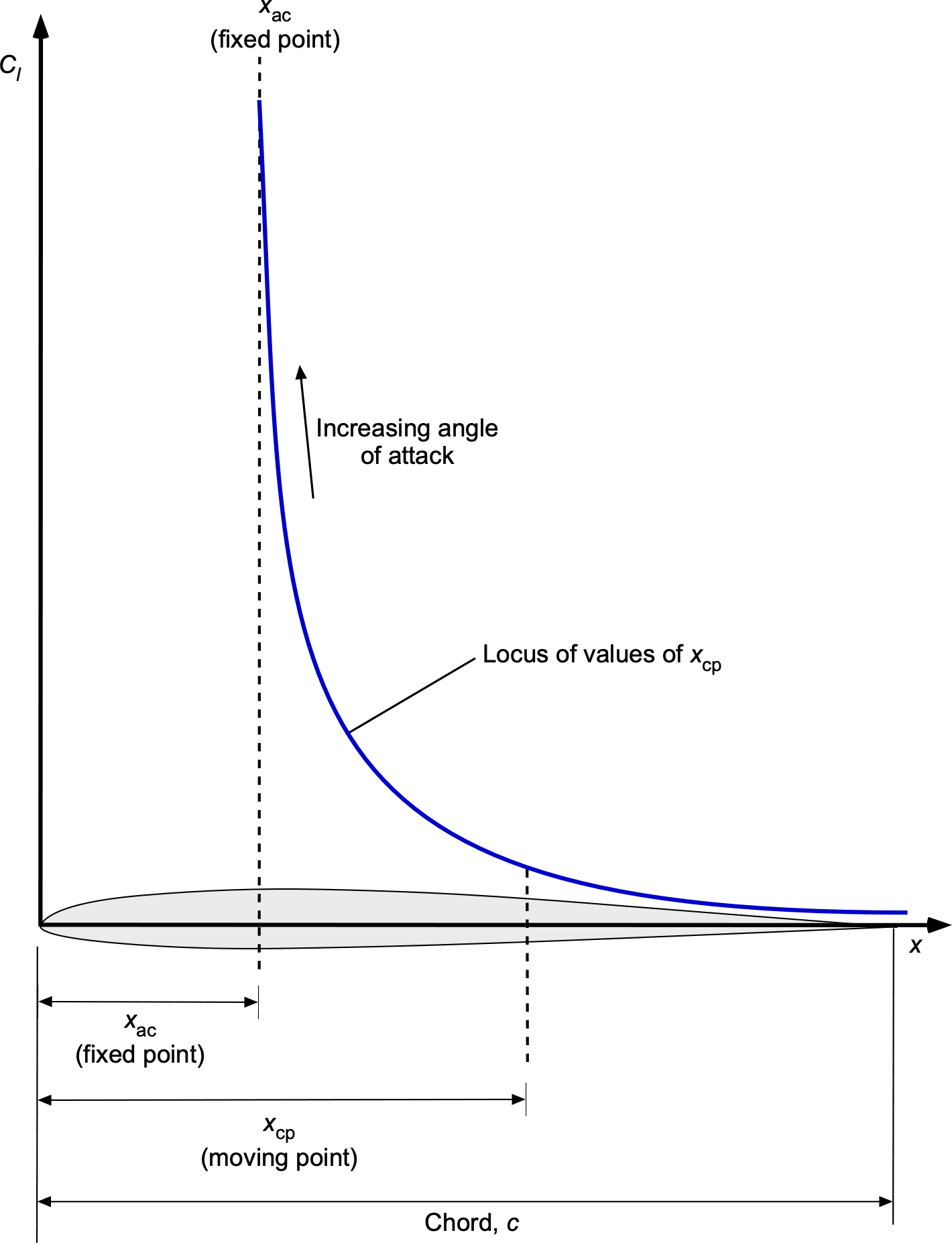
For a symmetric airfoil, then
(139) 
so the aerodynamic center and the center of pressure coincide. For a cambered airfoil, then
(140) 
which shows that the aerodynamic center remains fixed at the 1/4-chord. However, for a cambered airfoil varies with according to Eq. 138.
Comparison with Moment Measurements
Airfoil measurements are usually presented about the 1/4-chord. In this regard, the pitching moment about the 1/4-chord can be obtained using the principles of statics, i.e.,
(141) 
noting that moments are measured as positive nose-up. Therefore,
(142) 
which is plotted below. Notice that the thin airfoil results tend to follow a slightly positive slope.
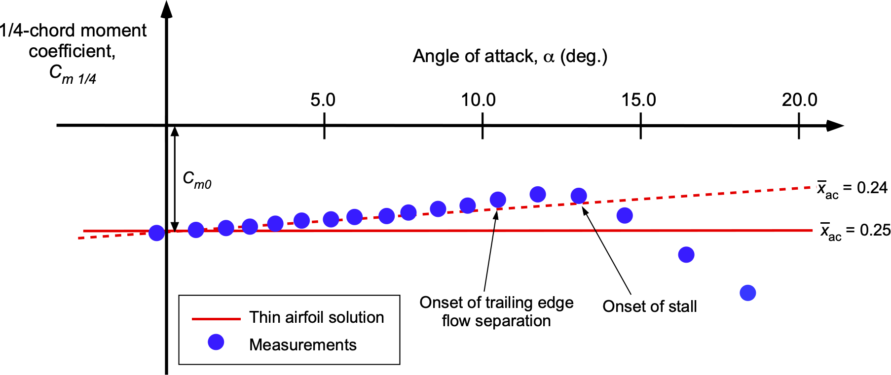
The pitching moment coefficient can also be written as
(143) 
where is the moment coefficient at zero-lift and  now becomes the actual position of the aerodynamic center other than at 1/4-chord. For these data, the actual aerodynamic center appears to be slightly forward of the 1/4-chord location. In general, the thin-airfoil theory aligns well with measurements of the zero-lift moment. However, minor deviations as a function of the angle of attack (or lift coefficient) indicate that the aerodynamic center is not perfectly at 1/4-chord for most airfoils. This outcome is because of the effects of viscosity and the formation of boundary layers on the upper and lower surfaces of the airfoil.
Check Your Understanding #1 – Aerodynamics of parabolic camberline
Determine the aerodynamic characteristics of a thin airfoil of unit chord, where the camberline is given by
![\[ y(x) = 4y_m x \left( 1 - x \right) \]](https://eaglepubs.erau.edu/app/uploads/quicklatex/quicklatex.com-321c66077b8cc1c50521048ced9d0df8_l3.svg "Rendered by QuickLaTeX.com")
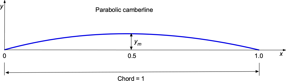
Show solution/hide solution.
The slope of the camberline is
![\[ \frac{dy}{dx} = 4y_m \left(1 - 2x\right) \]](https://eaglepubs.erau.edu/app/uploads/quicklatex/quicklatex.com-0e015883cebe80b0a9549d858ff55eed_l3.svg "Rendered by QuickLaTeX.com")
Substituting  gives
gives
![\[ \frac{dy}{dx} = 4y_m \left( 1 - 2\left(\frac{1}{2}(1 - \cos\theta)\right) \right) = 4y_m \cos\theta \]](https://eaglepubs.erau.edu/app/uploads/quicklatex/quicklatex.com-8df7bb1ceb92a59aade228837fd43f19_l3.svg "Rendered by QuickLaTeX.com")
The term is given by
![\[ A_0 = \alpha - \frac{1}{\pi} \int_0^\pi \frac{dy}{dx} \, d\theta = \alpha - \frac{1}{\pi} \int_0^\pi 4y_m \cos\theta \, d\theta = \alpha \]](https://eaglepubs.erau.edu/app/uploads/quicklatex/quicklatex.com-1315d50108652a7fe33cb46a43dc5916_l3.svg "Rendered by QuickLaTeX.com")
The term is given by
![\[ A_1 = \frac{2}{\pi} \int_0^\pi \frac{dy}{dx} \cos\theta \, d\theta = \frac{2}{\pi} \int_0^\pi 4y_m \cos^2\theta \, d\theta = \frac{2}{\pi} 4y_m \int_0^\pi \frac{1 + \cos(2\theta)}{2} \, d\theta \]](https://eaglepubs.erau.edu/app/uploads/quicklatex/quicklatex.com-9b66e5f9e7aa9f4856a7a534337c7ce2_l3.svg "Rendered by QuickLaTeX.com")
Separating the integral gives
![\[ A_1 = \frac{2}{\pi} 4y_m \left( \int_0^\pi \frac{1}{2} \, d\theta + \int_0^\pi \frac{\cos(2\theta)}{2} \, d\theta \right) \]](https://eaglepubs.erau.edu/app/uploads/quicklatex/quicklatex.com-27abfc89bad716e7cf236b7113a6a5fa_l3.svg "Rendered by QuickLaTeX.com")
Because  , it simplifies to
![\[ A_1 = \frac{2}{\pi} 4y_m \left( \frac{\pi}{2} \right) = 4y_m \]](https://eaglepubs.erau.edu/app/uploads/quicklatex/quicklatex.com-a204fcb0666b5d5aa36beefb86566a28_l3.svg "Rendered by QuickLaTeX.com")
The lift coefficient is given by
![\[ C_l = 2\pi \left( A_0 + \dfrac{A_1}{2} \right) = 2\pi \left( \alpha + 2y_m \right) \]](https://eaglepubs.erau.edu/app/uploads/quicklatex/quicklatex.com-49795112b174f01ea942206d29eeb7a7_l3.svg "Rendered by QuickLaTeX.com")
The moment about the leading edge (LE) is given by
![\[ C_{m,\text{LE}} = -\frac{\pi}{2} \left( A_0 + A_1 \right) = -\frac{\pi}{2} \left( \alpha + 4y_m \right) = -\frac{\pi}{2} \alpha - 2\pi y_m \]](https://eaglepubs.erau.edu/app/uploads/quicklatex/quicklatex.com-24bfcf848a24921f161a1818a754ce73_l3.svg "Rendered by QuickLaTeX.com")
The moment about the quarter-chord ( ) is given by
![\[ C_{m,\frac{c}{4}} = -\frac{\pi}{4} A_1 = -\frac{\pi}{4} 4y_m = -\pi y_m \]](https://eaglepubs.erau.edu/app/uploads/quicklatex/quicklatex.com-5d586e7499c7064e65a72baff2954671_l3.svg "Rendered by QuickLaTeX.com")
Check Your Understanding #2 – Analysis of a two-part camberline
Consider a NACA 2415 airfoil two-part camberline given by
![\[ \frac{y_c}{c} = \begin{cases} \dfrac{2m}{p^2} \left(p - \dfrac{x}{c}\right) \dfrac{x}{c}, & 0 \leq \dfrac{x}{c} \leq p \\[16pt] \dfrac{2m}{(1-p)^2} \left(\dfrac{x}{c} - p\right) \left(1 - \dfrac{x}{c}\right), & p \leq \dfrac{x}{c} \leq 1 \end{cases} \]](https://eaglepubs.erau.edu/app/uploads/quicklatex/quicklatex.com-9f78de347a8b615dc755444ec9bbdc29_l3.svg "Rendered by QuickLaTeX.com")
where  (maximum camber),
  (location of maximum camber as a fraction of chord),
  (chord length). The airfoil operates at an angle of attack
  . Using the thin airfoil theory:
- Calculate the lift coefficient, .
- Determine the moment coefficient about the aerodynamic center,
 .
. - Find the moment coefficient about the leading edge, .
Show solution/hide solution.
The slope of the camberline is obtained by differentiating  with respect to . For the two segments:
![\begin{align*} \text{\small For } 0 \leq \frac{x}{c} \leq p: & \quad \frac{dy_c}{dx} = \frac{2m}{p^2} \left(p - 2\frac{x}{c}\right), \\[12pt] \text{\small For } p \leq \frac{x}{c} \leq 1: & \quad \frac{dy_c}{dx} = \frac{2m}{(1-p)^2} \left(2\frac{x}{c} - p - 1\right). \end{align*}](https://eaglepubs.erau.edu/app/uploads/quicklatex/quicklatex.com-3996d0dab3ddbe00e35242b6c9d7f6e2_l3.svg "Rendered by QuickLaTeX.com")
Substituting and , gives
![\begin{align*} \text{\small First segment: } & \quad \frac{dy_c}{dx} = 0.25 \left(0.4 - 2\frac{x}{c}\right) \\[12pt] \text{\small Second segment: } & \quad \frac{dy_c}{dx} = 0.555 \left(2\frac{x}{c} - 1.4\right) \end{align*}](https://eaglepubs.erau.edu/app/uploads/quicklatex/quicklatex.com-8e96ea67c5b2823a252fcf8a46475098_l3.svg "Rendered by QuickLaTeX.com")
The lift coefficient is given by
![\[ C_l = 2\pi \alpha + 2\pi \left(\frac{m}{p} - \frac{m}{1-p}\right) \]](https://eaglepubs.erau.edu/app/uploads/quicklatex/quicklatex.com-2ea7ef8683f693e3ad0823d0756ff4a5_l3.svg "Rendered by QuickLaTeX.com")
Substituting the known values gives
![\[ C_l = 2\pi (0.0873) + 2\pi \left( \frac{0.02}{0.4} - \frac{0.02}{0.6}\right) = 0.653 \]](https://eaglepubs.erau.edu/app/uploads/quicklatex/quicklatex.com-cfdd344cfb8ce52245e9be44e185706d_l3.svg "Rendered by QuickLaTeX.com")
The moment coefficient about the aerodynamic center is
![\[ C_{m,\text{ac}} = -\pi \left( \frac{m}{p} - \frac{m}{1-p} \right) = -\pi \left( 0.05 - 0.0333 \right) = -0.0524 \]](https://eaglepubs.erau.edu/app/uploads/quicklatex/quicklatex.com-36a59e9008dec3769aa007bb2cd828f9_l3.svg "Rendered by QuickLaTeX.com")
The moment coefficient about the leading edge is
![\[ C_{m,\text{LE}} = C_{m,\text{ac}} + \frac{1}{4}C_l = -0.0524 + \frac{1}{4}(0.653) = 0.1106 \]](https://eaglepubs.erau.edu/app/uploads/quicklatex/quicklatex.com-b33189ee6c81c7b2fe2b4481bea81107_l3.svg "Rendered by QuickLaTeX.com")
Zero-Lift Angle of Attack
The lift coefficient of a cambered airfoil is given by
(144) 
where is called the zero-lift angle of attack. For a symmetric airfoil,  , and for a cambered airfoil the thin airfoil theory gives
(145) 
The zero-lift angle is usually a small negative number for most airfoils, as shown in the figure below. The camber shifts the lift curve upward on the plot, meaning that a cambered airfoil must have its angle of attack depressed to a lower value for no lift generation.
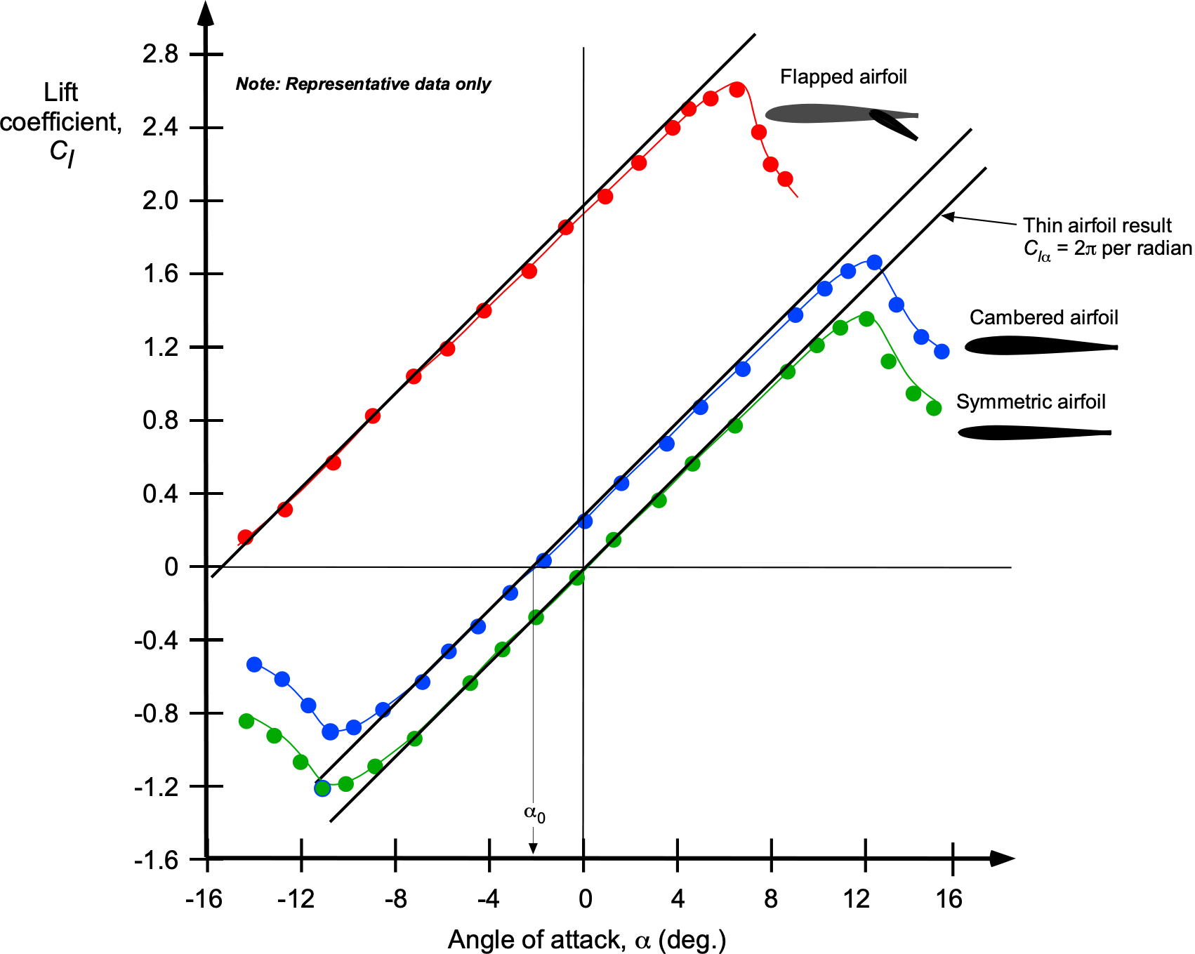
Airfoil with a Flap
An airfoil with a flap is a standard aerodynamic configuration that controls lift and pitching moments. The geometry of this configuration is shown in the figure below. The value of  represents the non-dimensional hinge point of the flap. It is the location along the chord line, measured as a fraction of the chord length, where the flap is hinged. The flap deflection angle,
  , is small and measured in radians. Positive values of indicate a downward deflection of the flap, increasing the camber of the airfoil.
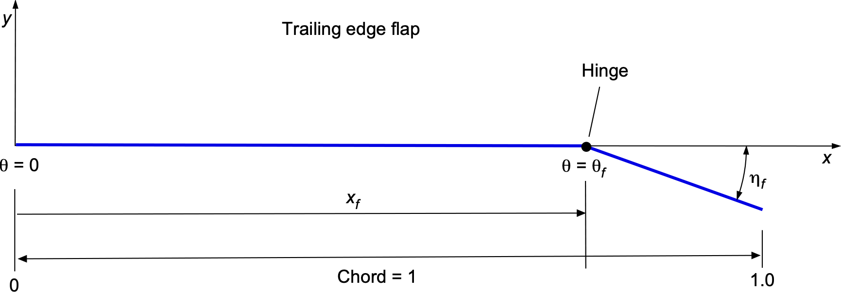
The slope of the camberline, which describes the shape of the airfoil’s mean camber, is
(146) ![\begin{equation*} \frac{dy}{dx} = \begin{cases} 0 & \text{for } 0 \leq x \leq x_f \\[9pt] \eta_f & \text{for } x_f \leq x \leq 1 \end{cases} \end{equation*}](https://eaglepubs.erau.edu/app/uploads/quicklatex/quicklatex.com-9e458b5e04b215335402d251caf3bd2a_l3.svg "Rendered by QuickLaTeX.com")
The camberline is flat, i.e.,  , from the leading edge to the flap hinge point, , and then it has a constant slope of from the hinge point to the trailing edge. Notice that
  is the angular location of the flap hinge, determined by the hinge location .
The Fourier coefficients for the camberline slope are found by integrating over the range ![[\theta_f, \pi]](https://eaglepubs.erau.edu/app/uploads/quicklatex/quicklatex.com-347ff21afb0b8b54dd25c1608d65a131_l3.svg "Rendered by QuickLaTeX.com") , giving
, giving
(147) 
and so for and  , then
(148) 
The lift coefficient is given by
(149) 
The moment coefficient about the leading edge is given by
(150) 
and the moment coefficient about the quarter-chord is given by
(151) 
Substituting the expressions for and  , gives
(152) 
This flap configuration is widely used in aircraft control surfaces, such as elevators, ailerons, and flaps, and can be optimized for specific flight conditions or performance goals. Notice that lift increases from the contributions from and , capturing the effect of flap deflection and hinge location  . The leading-edge moment reflects the influence of flap deflection. Smaller values of (hinge near trailing edge) increase flap effectiveness, while larger values of (hinge closer to the leading edge) reduce it.
Modeling Drag
In potential flow, which assumes an inviscid, irrotational, and steady fluid, drag is theoretically absent, which, as previously discussed, is known as d’Alembert’s paradox. This outcome occurs because the pressure distribution around a body in such a flow is chordwise symmetric, resulting in no net force opposing motion. Potential flow does not account for effects such as viscosity or flow separation, which contribute to drag. Consequently, while potential flow theory is insightful for understanding flow patterns and lift, it cannot predict drag. Therefore, according to the thin airfoil theory, the drag on an airfoil is zero.
Viscous effects must be considered to address this limitation. The problem has two aspects: 1. The effects of viscosity on pressure drag. 2. The production of shear (skin friction) drag. At a minimum, the boundary layer theory must be used to model the effects of viscosity near the surface to obtain the skin-friction drag and the pressure drag because of boundary-layer displacement effects.
For the pressure drag, consider the following approach by resolving the components of the normal force and axial chord force (or leading edge suction force) through the angle of attack, i.e., in the coefficient form, then
(153) 
where  is the normal force coefficient, and
  is the leading edge suction force, as shown in the figure below. Notice that the normal force acts normal or perpendicular to the airfoil’s chord, and the leading edge suction force acts parallel to the chord.
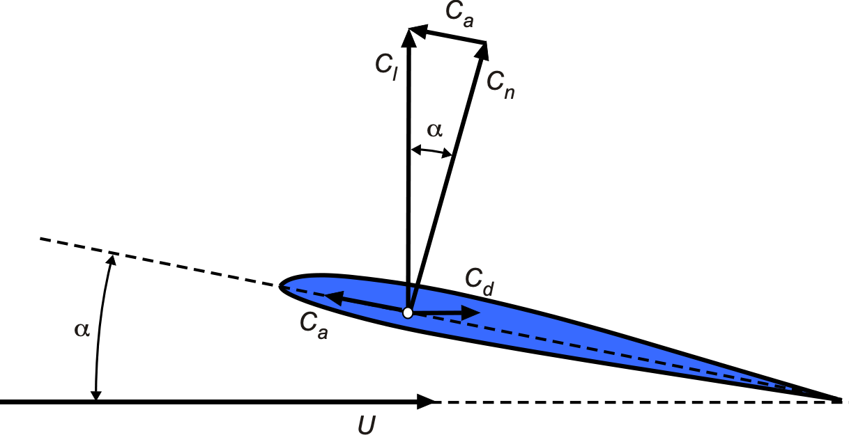
The general expression to determine the leading edge suction force is
(154) 
which is a limiting process because of the singular nature of the pressure at the sharp leading edge.[13] A formal theoretical derivation of this result involves the integration of the pressure singularity around the leading edge, which gives a finite suction force proportional to the square of the leading edge singularity. In essence, the term  arises in calculating the suction force because the suction force depends on the localized energy density contribution near the leading edge. Dynamic pressure is proportional to the square of the velocity, i.e.,
  . From Bernoulli’s equation, velocity differences in the flow correspond to pressure differences, i.e.,
  . Therefore, is proportional to the energy contribution per unit area (pressure difference squared).
The thin airfoil theory gives the chordwise pressure distribution as
(155) 
so the leading edge suction force is
(156) 
which gives
(157) 
The pressure drag can now be obtained by force resolution using
(158)
where to a small angle approximation  ,
,  , and
, and  . Therefore,
(159) 
which, as expected, is zero for a potential flow.
However, in a real flow, the effects of finite airfoil shape and viscosity are expected to limit the leading-edge suction pressure to a value below the theoretically achievable level, as shown in the figure below. This effect can be represented using a leading edge suction efficiency or recovery factor,  , such that
  . In this case, then
(160) 
Therefore, the pressure drag is non-zero in an actual flow, as expected, and increases proportionally with  , i.e., quadratically. Notice that if
  , then
  , thereby recovering the potential flow solution.
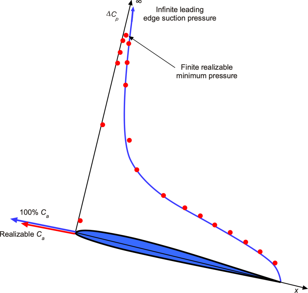
However, the limitation of this approach is that the value of is not known a priori and must be assumed or estimated. Experience with drag modeling on airfoils suggests that  0.95 for airfoils with low to moderate values of the thickness-to-chord ratio, i.e.,
  0.12, and lower for airfoils with greater thickness and/or a larger nose radius.
In general, for a cambered airfoil then  , so that the drag is
(161) 
and collecting the other terms gives
(162) 
(163) 
Equation 163 is a good approximation to the pressure drag behavior with the angle of attack of most airfoils in the low-speed flow regime, which is referred to as the “Modified thin airfoil theory” shown in the figure below.
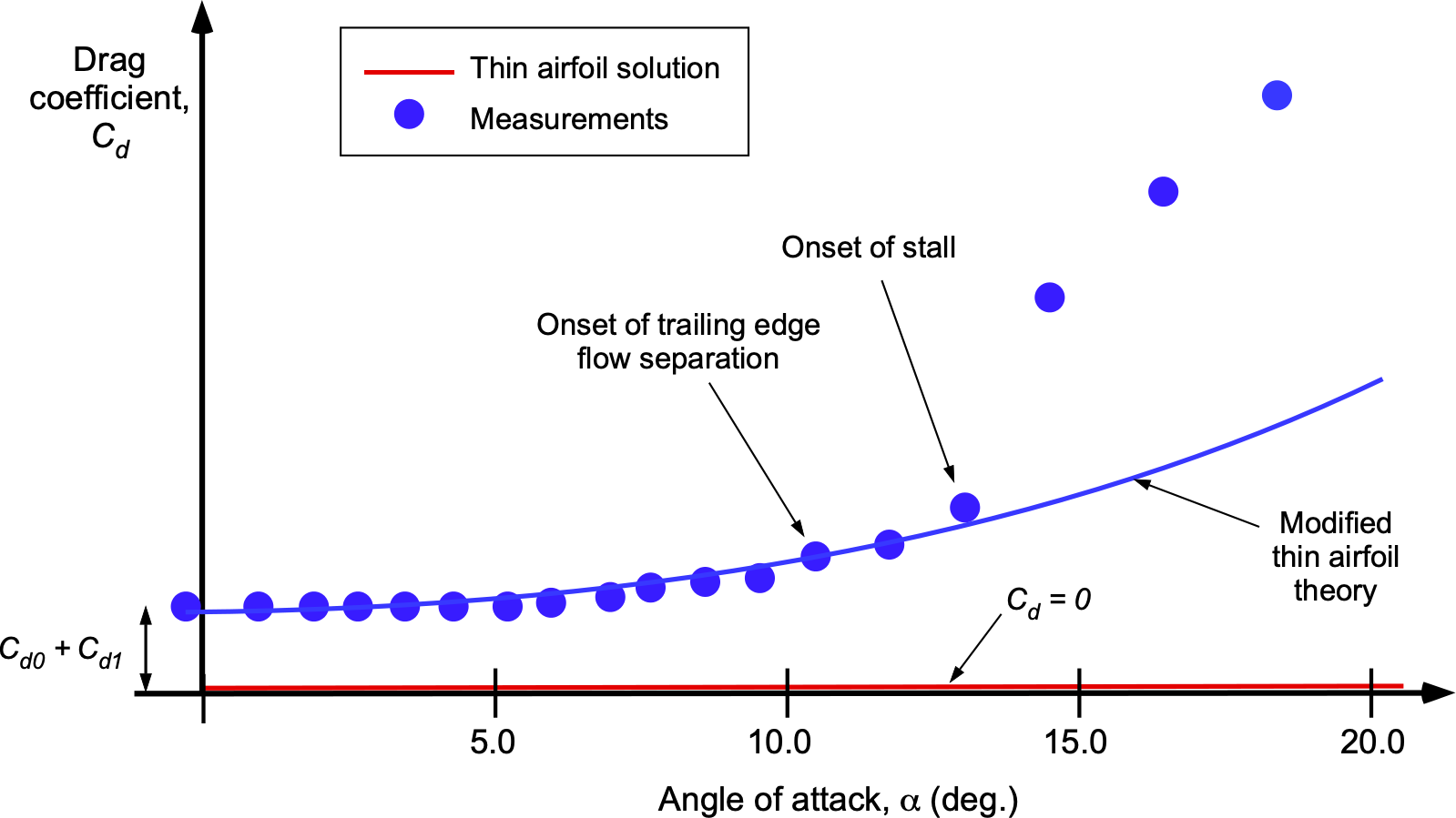
The effect of viscous shear drag (boundary layer drag) can be approximated by adding another (constant) term,  , i.e.,
(164) 
Equation 164 is valid only in the regimes where the flow is fully attached. This result also applies to higher chord Reynolds numbers, where the boundary layer is thinner and conforms closely to the airfoil surface. Notice that  for a symmetric airfoil because , so that
(165) 
It will be apparent that a drag model, such as Eq. 164, is not predictive but postdictive, i.e., it is an after-the-fact model. More advanced models, such as XFOIL, could be used to find the coefficients, including . These coefficients can also be found by fitting Eq. 164 from wind tunnel data. However, in terms of an initial predictive capability, it will be sufficient to assume that  0.95 for airfoils with low to moderate values of the thickness-to-chord ratio, i.e., 0.12.
Inverse Airfoil Design
Inverse airfoil design involves determining the shape of an airfoil based on a desired aerodynamic goal, such as a pressure distribution,  , the idea being outlined in the figure below. Constraints will also be imposed, both aerodynamic and geometric. For example, an aerodynamic constraint may limit the pitching moment about some axis. A geometric constraint may be the minimum or maximum camber or net thickness. The process is performed iteratively, and careful attention must be paid to convergence.
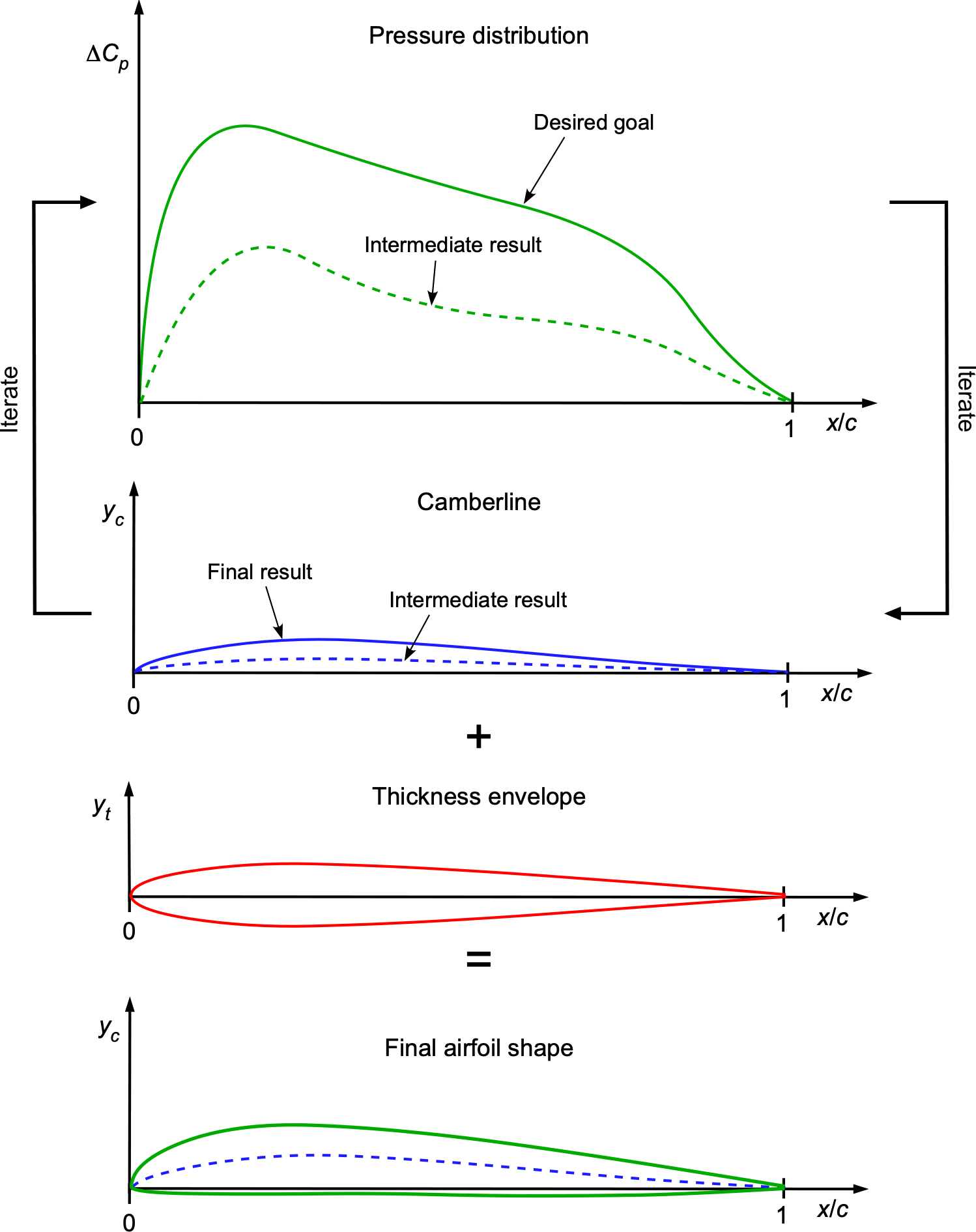
Starting from the fundamental equation of thin airfoil theory, i.e.,
(166) 
which can be written in terms of the pressure coefficient as
(167) 
The initial slope of the camberline,  , is determined from the desired differental pressure coefficient distribution about some reference angle of attack using the equation
(168) 
The process can be conducted numerically for discrete values of . Sometimes, a characteristic camberline may need to be specified, such as parabolic, cubic, or two-part, and the iteration is performed with the camberline coefficients rather than the camberline shape itself. Notice that in the thin airfoil theory, only the differential pressure, i.e., the difference in pressure between the lower and upper surfaces, can be predicted for the desired operating angle of attack.
Once a first approximation to the slope is obtained, the camberline,  , is obtained by integration using
(169) 
which can again be done numerically for each  value across the chord. These latter two steps are then repeated to achieve convergence.
The airfoil shape is then defined in terms of the upper and lower surfaces by adding the thickness envelope, i.e.,
(170) 
where  is the upper surface of the airfoil and
  is the lower surface. The thickness distribution,
  , is typically predefined or derived from airfoil thickness equations, such as the NACA 00XY thickness functions. While a thickness envelope is usually distributed normally (perpendicular) to the camber, when the camberline is thin, there is no practical difference in the resulting airfoil shape.
Of course, this thin-airfoil approach only approximates the required shape. The theory’s linearization assumptions lead to greater uncertainty in shape prediction as the camberline slope increases. Still, it often provides a good initial shape for further design optimization, such as using a surface singularity (panel) method or a computational fluid dynamics (CFD) method.
Summary & Closure
Conformal mapping offers a powerful approach to analyzing idealized aerodynamic flows. Using analytic functions, flows such as uniform flow around a circle can be mapped into flows around airfoil-like shapes. The Joukowsky and Kármán-Trefftz transformations enable the derivation of exact solutions for the flowfield. These methods account for circulation and enforce the Kutta condition at the trailing edge, yielding predictions of the flowfield and the forces and moments. Because the entire flow field is analytically described, conformal mapping provides considerable insight into how geometry affects the flow around an airfoil.
Thin airfoil theory, while limited to the evaluation of integrated quantities, offers a practical and elegant route to estimating the aerodynamic forces and moments on airfoils. The airfoil is represented as a bound vortex sheet whose strength is determined by satisfying the flow tangency condition along the camber line. This approach leads to closed-form expressions and predicts a lift slope of per radian of angle of attack, with the aerodynamic center being at the quarter-chord. However, the assumptions behind thin airfoil theory impose clear limitations, and it cannot predict drag, flow separation, or stall. Compressibility is also often ignored, although modest corrections, such as the Prandtl-Glauert transformation, can extend its usefulness to subsonic flows.
5-Question Self-Assessment Quickquiz
For Further Thought or Discussion
- How does the camberline shape affect the lift slope and moment coefficients in thin airfoil theory?
- What role does the camber distribution play in determining the zero-lift angle of attack for a cambered airfoil?
- How does thin airfoil theory account for pitching moments, and why is the moment coefficient about the leading edge different for symmetric and cambered airfoils?
- How does the thin airfoil theory lift slope of 2π per radian of the angle of attack compared with experimental data?
- What is the significance of the Kutta condition in thin airfoil theory, and how does it ensure a smooth trailing edge flow?
- How might the thin airfoil theory be applied to predict the aerodynamic performance of a multi-element airfoil system?
- Why does thin airfoil theory fail for thick or highly cambered airfoils, and what modifications might improve its applicability?
- According to Kelvin’s circulation theorem, circulation is a conserved quantity. Consider what happens to the flow at the trailing edge if an airfoil is set into impulsive motion and suddenly stops again.
Other Useful Online Resources
To understand more about the thin airfoil theory and how to apply it, explore some of these online resources:
- A nice, clear video on the thin airfoil theory by Prof. Van Bren.
- Airfoil analysis, thin airfoil theory, & fundamental equation. Video by AeroAcademy.
- Applying thin airfoil theory: Step-by-step exercises | Aerodynamics Lecture.
- Solutions to thin airfoil theory | Aerodynamics Lecture 1.
- Solutions to thin airfoil theory | Aerodynamics Lecture 2.
- Kutta, M. W., "Auftrieb von Flügeln in strömender Flüssigkeit," Il Nuovo Cimento, Vol. 3, 1902. ↵
- Zhukovsky, N. E., "Über die Konturen der Tragflächen der Drachenflieger," Trudy TsAGI, 1906–1910 (various parts). ↵
- Munk, Max M. (Max Michael), "Isoperimetrische Aufgaben aus der Theorie des Fluges." Göttingen, Dieterichsche Universitäts-Buchdruckerei, 1919, 31 pp. (Doctoral dissertation, Georg-August-Universität Göttingen). ↵
- Glauert, H., "The Elements of Aerofoil and Airscrew Theory," Cambridge University Press, 1926 ↵
- Notice that lowercase subscripts always indicate the application to a two-dimensional wing or airfoil section. ↵
- Other than the effects of viscosity, this flow is equivalent to a singularity in potential flow. ↵
- It cannot be ignored in an unsteady flow analysis, which opens up the field of unsteady aerodynamic theory. ↵
- Time is measured non-dimensionally in terms of chord lengths of airfoil travel, which must approach 10 to reach the steady state. ↵
- Theodorsen, T., & Garrick, I. E., " Theory of Airfoils of Arbitrary Shape," NACA Report No. 659. ↵
- . Theodorsen, T., "General Potential Theory of Arbitrary Wing Sections," NACA Report No. 411, 1931; also: "Theory of Aerodynamic Lift," NACA Report No. 496, 1935. ↵
- Schwarz, H. A., "Über einige Abbildungsaufgaben,'' Journal für die reine und angewandte Mathematik, Vol. 70, pp. 105–120, 1869; Christoffel, E. B., "Über die Transformation der elliptischen Integrale," ibid., pp. 46–70.} ↵
- Bairnbaum, W, "Die tragende Wirbelfläche als Hilfsmittel zur Behandlung des ebenen Problems der Tragflügeltheorie," ZAMM, 1923, 3, pp. 290–297. ↵
- Jones, R. T., "Leading-Edge Singularities in Thin-Airfoil Theory," Journal of the Aeronautical Sciences, Vol. 17, No. 5, May 1950. ↵
