33 Aerodynamics of Airfoil Sections
Introduction
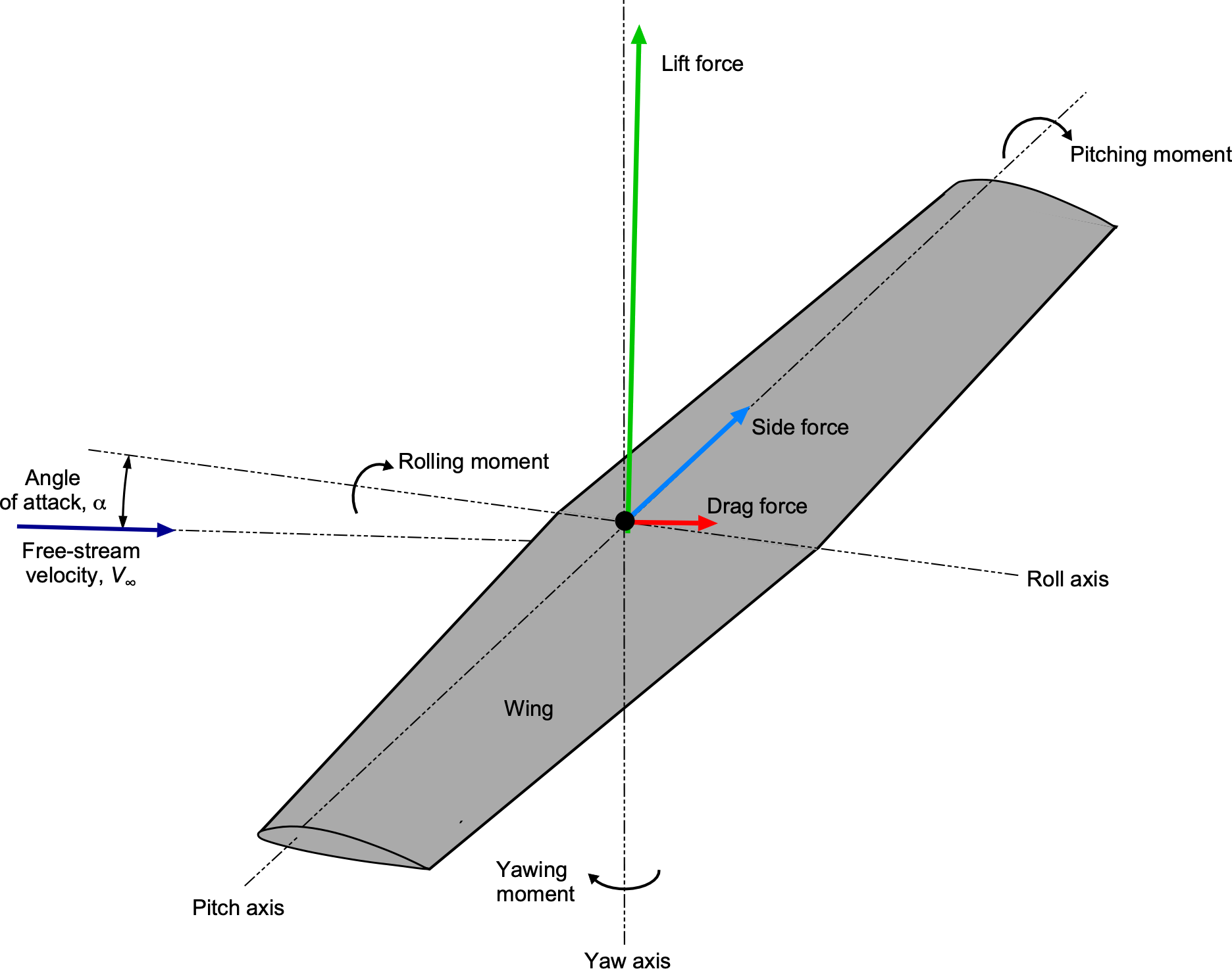
Understanding the aerodynamic behavior of airfoils and wings, often referred to as lifting surfaces, is a crucial aspect of aerospace engineering practice and essential for the successful design of all aircraft. Any lifting surface that moves through a fluid will experience some form of fluid-dynamic force. By definition, the component of this force that acts on the surface in a direction perpendicular to the relative freestream velocity,  , or “relative wind direction”[1] is called the lift, as shown in the figure below. The force component on the surface, acting in a direction parallel to the relative wind, is called drag. The magnitude of the lift and drag forces depends on several factors, including the size and shape of the lifting surface, its orientation to the flow, the flight Reynolds number (based on a characteristic length), and the freestream Mach number. Moments can also be produced on the lifting surface about each of the longitudinal, lateral, and vertical axes.
However, before examining the characteristics of finite wings, i.e., three-dimensional wings with finite span and perhaps with twist, planform taper, and thickness variations, it is prudent to investigate the aerodynamic characteristics of two-dimensional airfoil sections. Such two-dimensional or “2-D” airfoils are equivalent to wings with infinite span and aspect ratio, where the aspect ratio indicates the slenderness of the wing. While the concept of a 2-D wing section may initially sound somewhat artificial, it is possible to mimic a wing of infinite aspect ratio, both experimentally and theoretically, and obtain aerodynamic results that pertain only to the shape of the airfoil section itself. Furthermore, this approach enables the isolation of other, more complex and interrelated effects associated with the finite span of a wing, including the impact of wing tip vortices and other aerodynamic effects caused by sweepback, twist, planform (chord) variations, and potentially other factors such as winglets.
Learning Objectives
- Be aware of the various definitions of aerodynamic forces and moments, as well as lift coefficient, drag coefficient, lift-curve slope, maximum lift coefficient, aerodynamic center, and center of pressure.
- Appreciate the effects of flaps and other high-lift devices on airfoil performance.
- Understand how to calculate the lift and other integrated quantities from the pressure and shear stress distributions about an airfoil.
- Know about the aerodynamic characteristics of airfoil sections, both in attached flow and with flow separation, and how these characteristics change at different Reynolds and Mach numbers.
Origin of Aerodynamic Forces
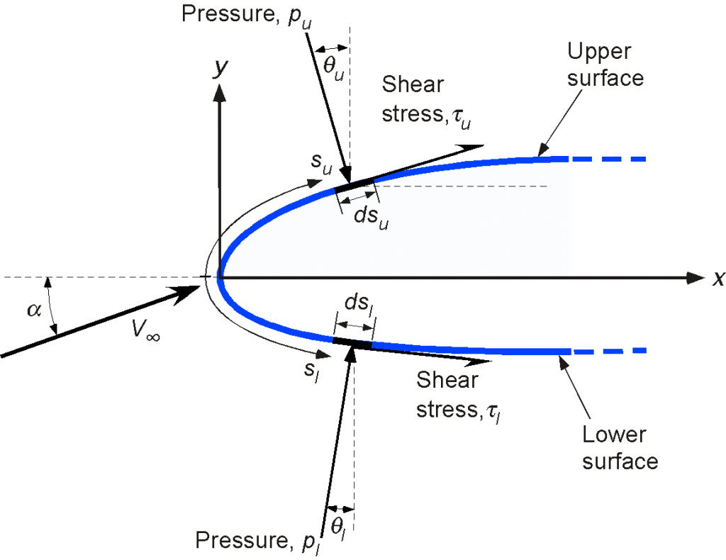
The origin of the net aerodynamic forces on an airfoil or wing, such as lift and drag, stems from the integrated effects of the pressure and boundary layer shear stress distributions acting over its surface, as illustrated in the figure below. These distributions, produced as the flow moves over the upper and lower surfaces, are nonuniform and can be either positive or negative. For example, higher pressure pushes inward toward the surface (as shown in red), while lower pressure pulls outward from the surface (as shown in green). Additionally, boundary-layer-induced shear stresses can be either positive (when the flow moves downstream) or negative (e.g., when the flow reverses).
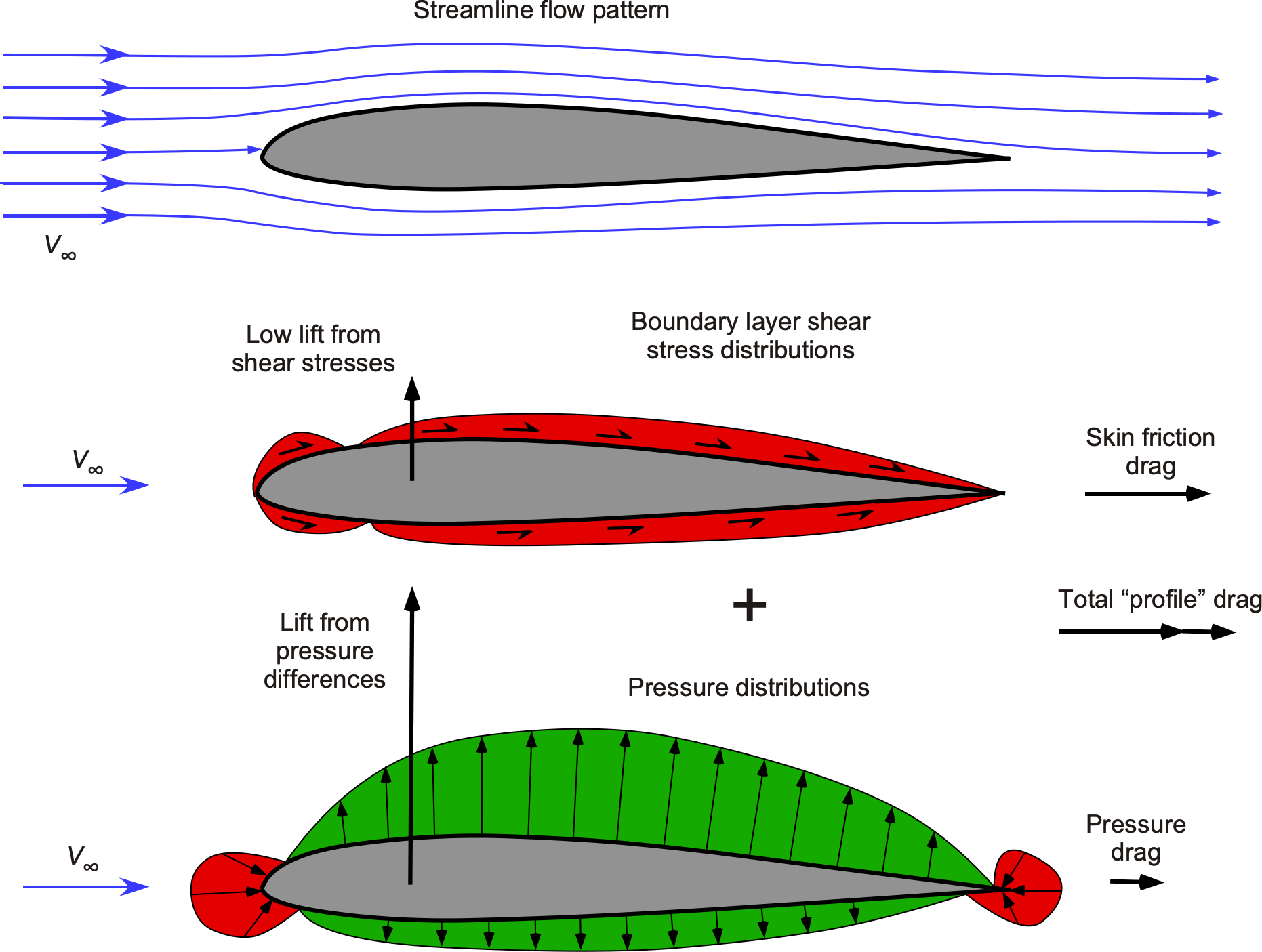
The figure above shows that the shear stresses in the aggregate act downstream, primarily parallel to the chord line. Hence, the net shear contributes significantly to the drag force on the airfoil section. Likewise, the differences in the pressure distribution between the upper and lower surfaces primarily contribute to the lift force and pitching moment on the airfoil, with shear stresses making a minor net contribution in the vertical direction.
In practice, the net forces and moments can be measured with a balance (e.g., a scale) or calculated by integrating the effects of the pressures and stresses acting on the surfaces. In the meantime, it is possible to proceed on the assumption that either measurement or calculation can be used to obtain these integrated results, with a particular approach detailed at the end of this chapter.
Two-Dimensional Flow
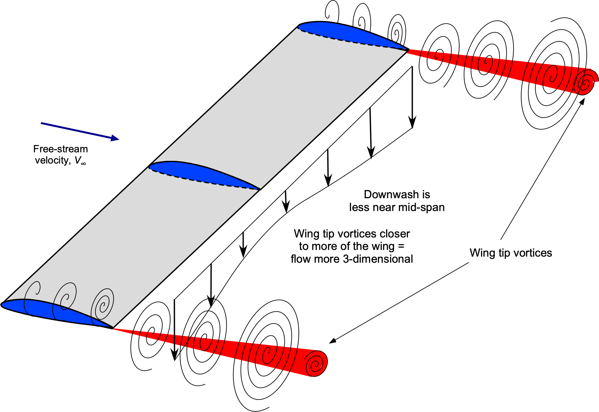
It should be appreciated that the flow over any wing of finite span will be inherently three-dimensional and further complicated by the effects of the vortices that trail behind the wing, as shown in the figure below. The presence of these vortices produces a downwash flow over the wing, affecting the local angles of attack over the entire wing and, therefore, its lift and overall aerodynamic characteristics. The flow can be assumed to be nominally two-dimensional (2-D) only at sections well away from the wingtip vortices, which would be at the mid-span.
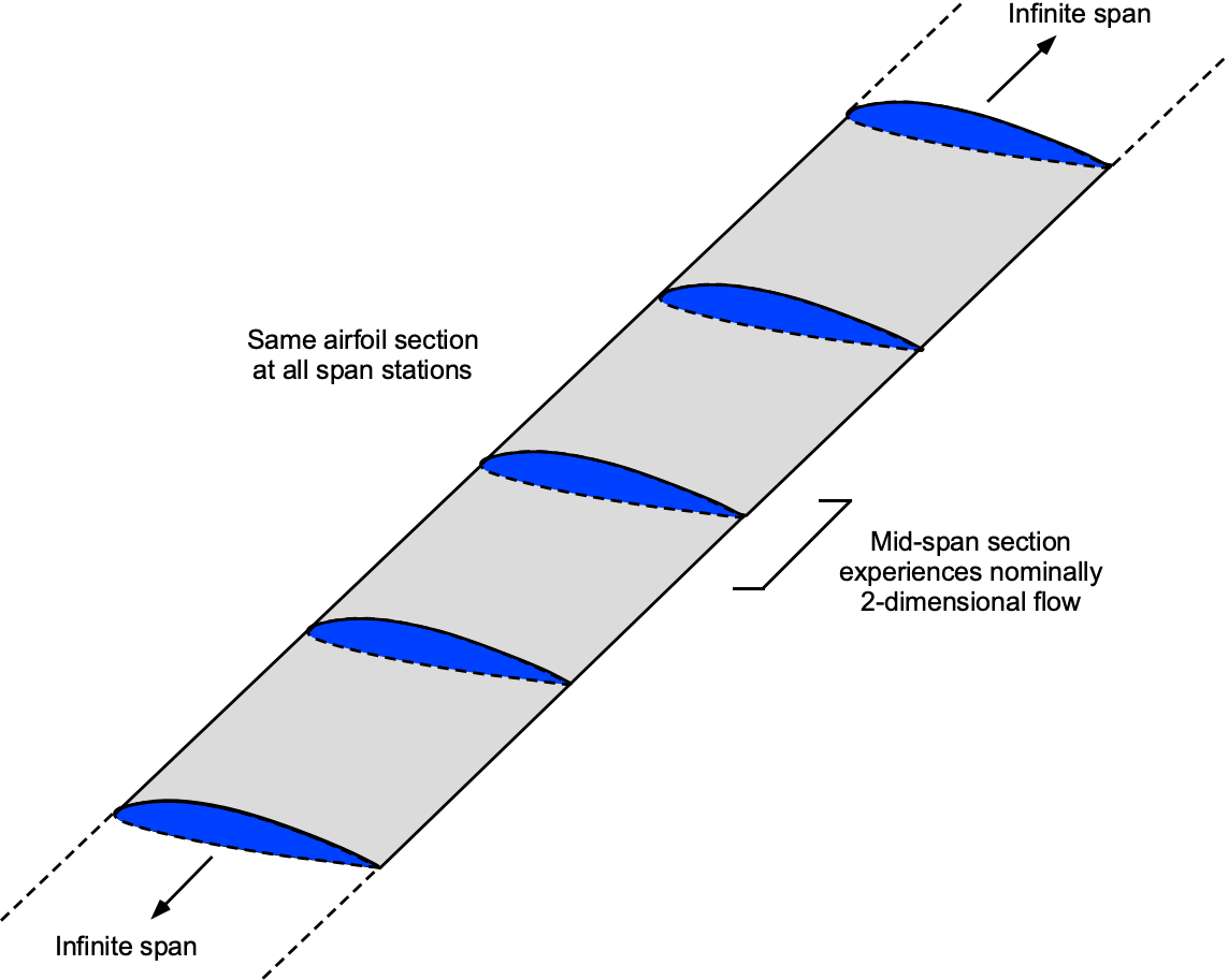
Initially, it is conceptually straightforward to understand the aerodynamic behavior of a wing by imagining the span and corresponding aspect ratio increasing without bound. In this idealized limit, the wingtip vortices are displaced so far from the central region that their influence becomes negligible, as shown in the figure below. Consequently, the flow over the mid-span can be treated as nominally two-dimensional. In this manner, it is possible to theoretically and experimentally mimic the behavior of 2-D wings, thereby deriving a better understanding of the aerodynamics of the airfoil section itself in isolation.
The term “nominally” must be used with caution, as a real flow can never be perfectly 2-D, regardless of how large the aspect ratio becomes. Still, the residual three-dimensional effects are reduced to a level that, for all practical purposes, can be regarded as insignificant. This approximation provides a sound foundation for further analysis of isolated airfoil aerodynamics.
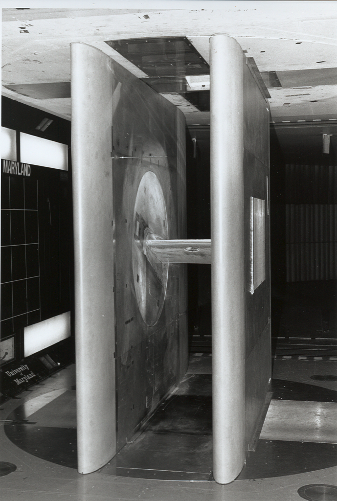
It is also possible to mimic an infinite span and aspect ratio in the wind tunnel. One approach is to span the wing from wall to wall, thereby preventing wake rollup at the tips and effectively eliminating the tip vortices. However, this approach not only requires a large wing but also promotes three-dimensional flow separation and the local formation of “stall cells” before stall onset. Another common practice is to test a short-span wing between two “false” walls, as shown in the photograph below. In wind tunnel terminology, this is referred to as a “2-D insert.” This particular approach has seen widespread use for testing 2-D airfoils, and flow visualization has confirmed the validity of the nominally 2-D flow development over the wing section at mid-span, at least up to the onset of stall. Post-stall, the flow always tends to become inherently more three-dimensional on any lifting surface, regardless of the test method used.
A key metric in two-dimensional airfoil performance is the maximum attainable lift coefficient,  . Despite advances in computational fluid dynamics (CFD), accurately predicting remains challenging, making wind-tunnel measurements indispensable. However, 2-D values of for the same airfoil section can vary significantly from one wind tunnel to another because of differences in their design, turbulence intensity, model aspect ratio, and wall interference effects. As previously mentioned, near the stall, three-dimensional flow phenomena frequently occur even in nominally 2-D tests, especially with longer-span airfoils. Hysteresis in stall behavior is also typical and often depends on whether the angle of attack is set before or after the wind tunnel is turned on. These factors underscore the importance of consistency in test methodology and adherence to standardized procedures when measuring 2-D airfoil characteristics.
Dynamic Pressure
The aerodynamic forces acting on a body are directly proportional to the dynamic pressure in the flow, which is the pressure associated with the fluid’s kinetic energy. Given the symbol  , dynamic pressure comes into most (if not all) aerodynamic problems. In general, the dynamic pressure is given by
(1) 
where  is the flow density, and
  is its velocity. Notice that dynamic pressure depends on the squared value of the flow speed. It can be easily confirmed that dynamic pressure has units of pressure, i.e., force per unit area, so that it will be expressed in base units of Nm
 (Pa) in the SI system or lb ft in the USC system.
In particular, the freestream dynamic pressure is defined as
(2) 
where  means conditions at “infinity” or just far away from the wing, where there is an undisturbed “freestream” flow. In practice, this point will be at least one chord length upstream of the airfoil. As will be shown, the freestream dynamic pressure
  is often used as the reference pressure in the definitions of most of the non-dimensional coefficients used in airfoil and wing aerodynamics.
Airfoil Forces and Moments
The resulting forces acting on an airfoil section from the integrated effects of the pressure and shear can be resolved into a wind-axis system (i.e., in terms of lift  and drag
  ) or a chord-axis system (i.e., in terms of normal force
  and a chord force
  ), as shown in the figure below. As previously discussed, an airfoil section can be considered a “2-D” wing. Therefore, for airfoils, dimensional force and moment quantities per unit span are used; i.e., the lift per unit span is written as
  /unit span = . This represents the lift force acting over a span of one unit. Furthermore, when force and moment coefficients are defined for airfoils, a reference length is needed, which is usually the chord length. In some cases, the semi-chord,
  , may be used as a reference length; however, this is less common, except in some advanced applications.
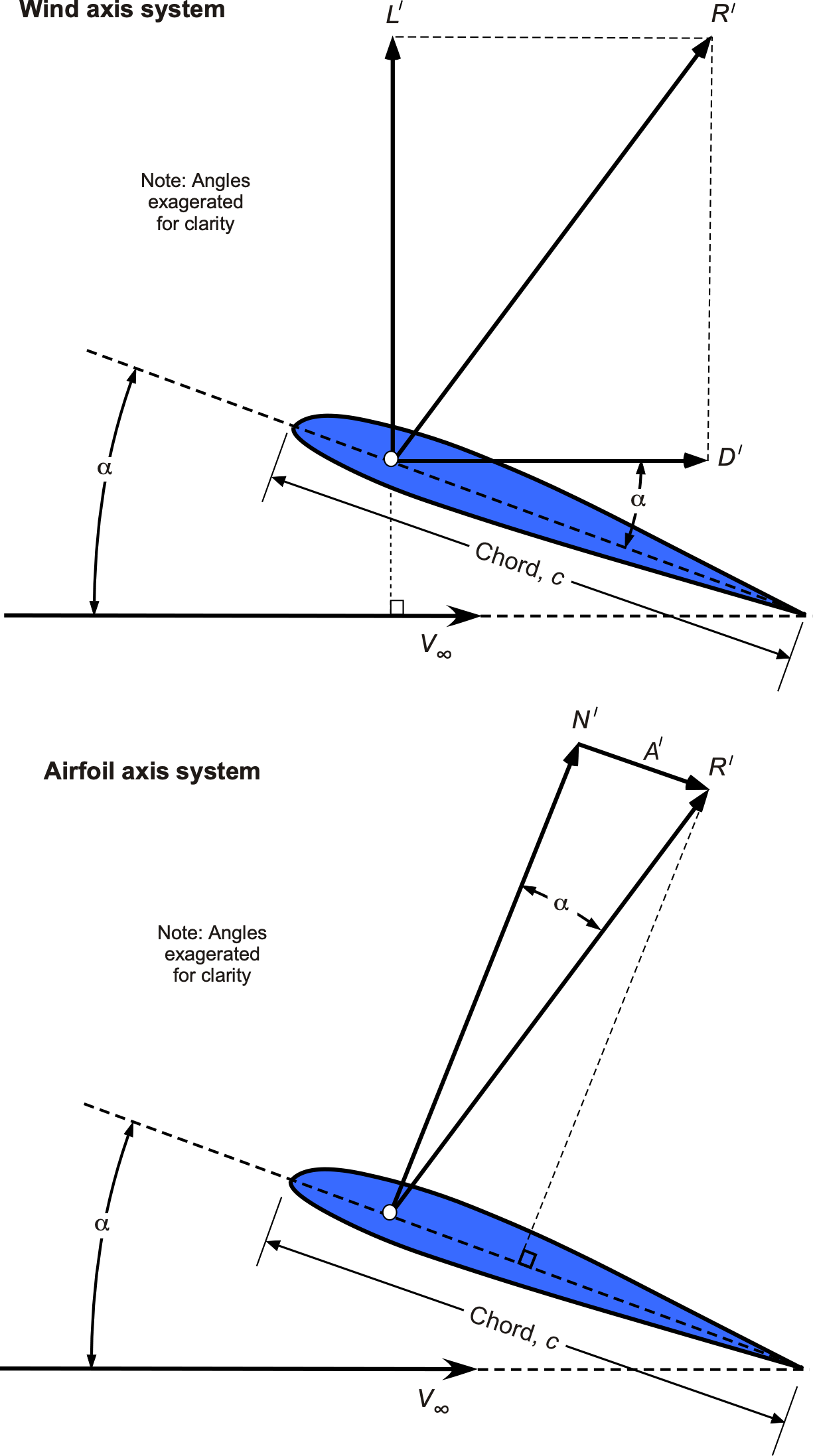
 . Two statically equivalent axis systems may be used.
By definition, the lift force or lift force per unit length, , acts in a direction that is perpendicular to the freestream velocity, . The corresponding drag  or drag per unit span, , is in a direction parallel to . Alternatively, the forces can be decomposed into the sum of two other forces, i.e., the normal force per unit span, , which acts normal (perpendicular) to the airfoil chord, and the leading-edge suction force or axial chord force per unit span, , which points toward the trailing-edge and acts parallel to the chord. Notice, however, that in some cases, the axial or chord force may be defined as positive when pointing toward the leading edge, so it is essential to know the sign convention being used.
Both of these latter force systems are useful in various analyses, although there is usually a preference for using lift and drag. It will be apparent from the preceding that the wind axis and body axis systems are statically equivalent, and one force system can be derived from the other through resolution using the angle of attack . For example, to transform from a body axis system ( and ) to a wind axis system ( and ), then
(3) ![\begin{eqnarray*} L' & = & N' \cos \alpha - A' \sin \alpha \\[8pt] D' & = & N' \sin \alpha + A' \cos \alpha \end{eqnarray*}](https://eaglepubs.erau.edu/app/uploads/quicklatex/quicklatex.com-4f81cad34be0a08eded83e9d9fbb41b8_l3.svg "Rendered by QuickLaTeX.com")
Alternatively, with the use of some trigonometry, transforming from a wind axis system ( and ) to a body axis system ( and ) gives
(4) ![\begin{eqnarray*} N' & = & L' \cos \alpha + D'' \sin \alpha \\[8pt] A' & = & D' \cos \alpha - L ' \sin \alpha \end{eqnarray*}](https://eaglepubs.erau.edu/app/uploads/quicklatex/quicklatex.com-0a9a3231be9ce669e4bb7acb35f0cdc9_l3.svg "Rendered by QuickLaTeX.com")
Aerodynamic Coefficients
Engineers must become familiar with how non-dimensional force and moment quantities are defined and applied to airfoils, wings, and other body shapes, as well as the specific values of these coefficients that have particular meanings. While dimensional forces (lb or N) and moments (ft-lb or N-m) are helpful in many forms of analysis, it is far more convenient to work with non-dimensional aerodynamic quantities, such as lift and drag coefficients.
For example, suppose the lift on a given wing is 900 N, and the corresponding drag is 30 N; these values are undoubtedly helpful to know. However, consider if the wing’s corresponding lift coefficient is 0.6 and its drag coefficient is 0.02. In that case, these values reveal much about the aerodynamic operating state of the airfoil, and the coefficients also allow comparisons of the effects of wings of different shapes and sizes. For this reason, airfoil data (measured or computed) are generally presented in terms of non-dimensional force and moment coefficients.
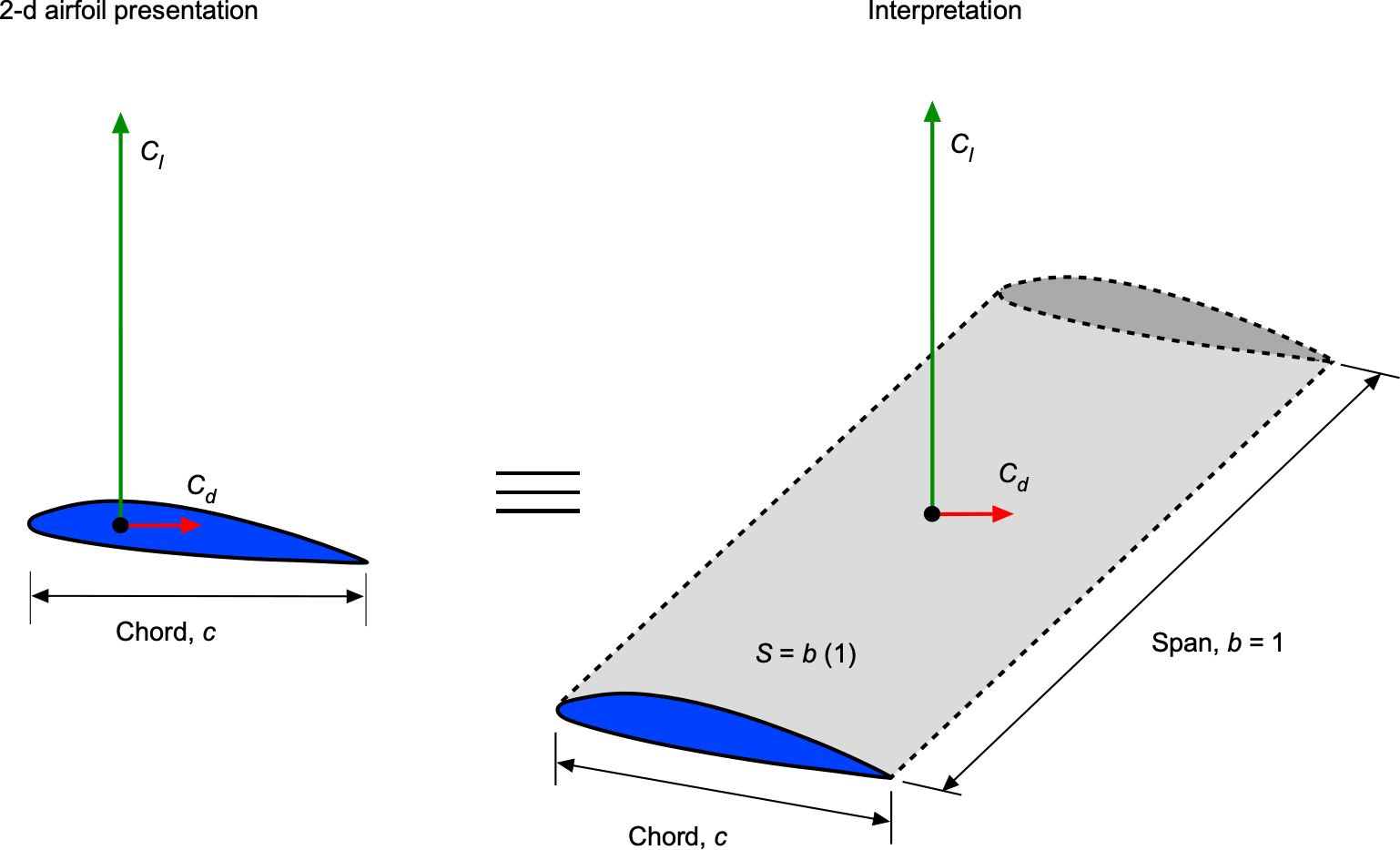
The airfoil section’s non-dimensional or dimensionless force coefficients are defined using the freestream dynamic pressure and chord  as a reference length. The span of a 2-D wing is infinite, so the aerodynamic forces and moments are referred to as per unit length or unit span of the wing, i.e., span = 1 unit, as illustrated in the figure below. A force is pressure times area, so the reference area of a force per unit span will be
  .
.
Therefore, the 2-D lift coefficient can be defined as
(5) 
where is the chord of the wing section or the airfoil, which is the distance from its leading edge to its trailing edge. Furthermore, it is assumed that the spanwise lift is uniform across the span, consistent with the 2-D assumption.
In summary, the 2-D force and moment coefficients can be written as:
Lift coefficient, 
 Drag coefficient,
Normal force coefficient, 
Axial (chord) force coefficient, 
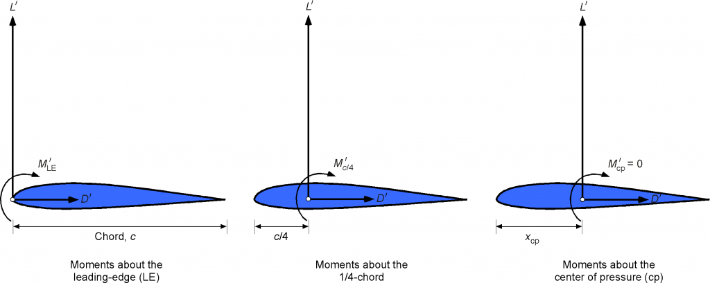
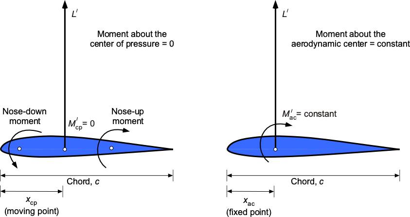
Pitching moments are defined as positive when they tend to increase the angle of attack of the airfoil section; thus, positive pitching moments are equivalent to nose-up moments. Again, the convention is that a moment  would represent a moment per unit span. Also, there are several convenient points about which the moments can be conveniently calculated, namely the leading edge (
 ), 1/4-chord (
 ), and the center of pressure
  , as shown in the figure below. Notice that when the reference point is moved to different locations on the chord, the values of the moments will change, but the forces acting at that point remain the same. i.e., there is no change in static force equilibrium.
The dimensionless moment coefficients for an airfoil section are defined as:
Moment coefficient at the leading-edge, 
Moment coefficient at some point  ,
, 
Moment coefficient at 1/4-chord, 
Moment coefficient at center of pressure, 
Notice the use of lower-case subscripts on all coefficients (e.g.,  , not
, not  , and
, and  , not
, not  ) when applied to a “2-dimensional” airfoil section. When applied to a finite-span wing, capital letter subscripts are used, as discussed later; this standard notation distinguishes the finite-span aerodynamic coefficients from those of 2-D airfoils.
Representative Aerodynamic Coefficients
The data shown in the plots below (indicated by the symbols) show measured values of the lift coefficient, , the drag coefficient, , and the 1/4-chord moment coefficient  as functions of the angle of attack for a NACA 23012 airfoil section in a low-speed flow. In this latter regard, a low-speed flow is at low Mach numbers where compressibility effects are relatively small. These results cover an angle-of-attack range from fully attached flow to the stalled flow condition. They are typical of the airfoil characteristics found in various standard catalogs, such as those from Abbott & Von Doenhoff. The results are often presented in relation to variations of the chord-based Reynolds number and/or the freestream Mach number.
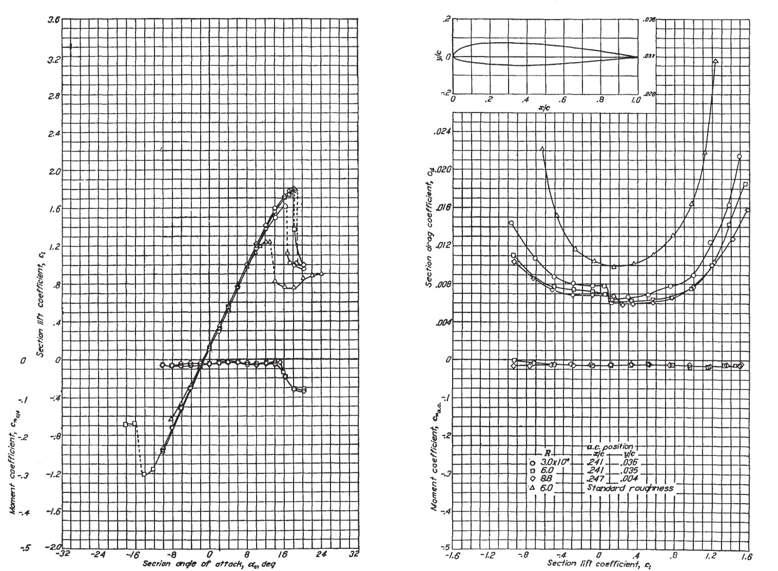 and 1/4-chord moment coefficient, versus angle of attack for a NACA 23012 airfoil, including the effects of surface roughness. The drag coefficient measurements, , are shown as a “polar” with respect to the values of the lift coefficient, .
Quantities such as maximum lift coefficient, minimum drag coefficient, maximum lift-to-drag ratio, pitching moments, and other metrics can all be significant in quantifying the aerodynamic characteristics of airfoils. These parameters can also be a basis for airfoil selection. However, interpreting the results from these preceding graphs and identifying relevant quantities requires some practice, as the overlap of many points and curves can be confusing. To this end, a more straightforward presentation is shown in the figure below, in which the lift coefficient , the moment coefficient about the 1/4-chord, , and the drag coefficient, , versus the angle of attack of the airfoil to the freestream flow, are more clearly delineated.
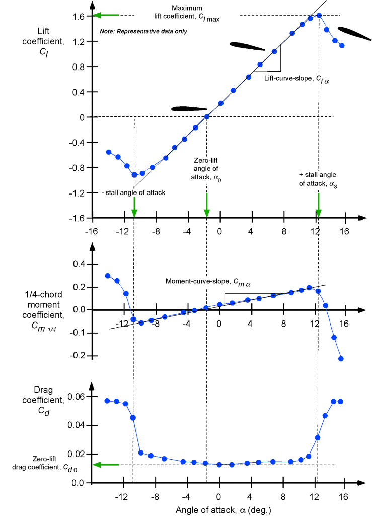 , the moment coefficient about the 1/4-chord, , and the drag coefficient, , versus the angle of attack.
At low angles of attack, the lifting characteristics of an airfoil are not significantly influenced by viscosity or the presence of boundary layers. Recall that boundary layers are thin, viscous-dominated regions near the surface. Notice that in this region, the lift coefficient increases almost in proportion to the angle of attack. The parameter  is the angle of attack for zero lift, or what is usually known as the zero-lift angle of attack. For a symmetric airfoil,
  ; for positively cambered airfoils, is usually a slight negative angle.
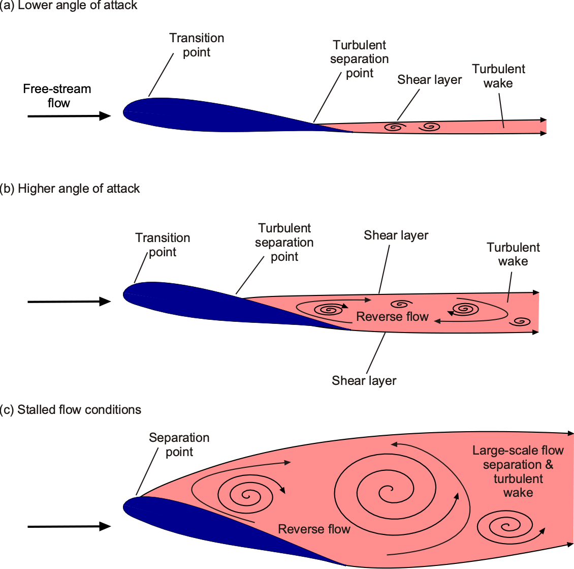
As the angle of attack increases, the boundary layer thickens, and the aerodynamic characteristics begin to exhibit nonlinear behavior. The airfoil will soon reach its maximum lift coefficient,  . A further increase in angle of attack leads to flow separation on the upper surface, a sudden loss of lift, and a significant increase in drag; this process is known as a stall. The flow also becomes unsteady at stall, as turbulence and vortices are shed from the airfoil’s upper surface, resulting in fluctuating aerodynamic forces.
The essential flow physics of the stall has been previously discussed and is illustrated schematically in the figure below. At low subsonic Mach numbers, the onset of stall usually occurs at an angle of attack between 12 and 15, depending on the airfoil section and the Reynolds number. Higher Reynolds numbers inevitably delay the onset of flow separation and stall, increasing the value of . Higher Mach numbers generally reduce the values of because of the higher adverse pressure gradients over the upper surface.
Pitching moments about the 1/4-chord are usually relatively low on most airfoils, but for a significantly cambered airfoil, as in the case shown, the moments will be non-zero. Often, the moment curve has a shallow positive slope because the aerodynamic center (defined later) is located close to, but just forward of, the 1/4-chord.
Check Your Understanding #1 – Obtaining airfoil characteristics from graphs
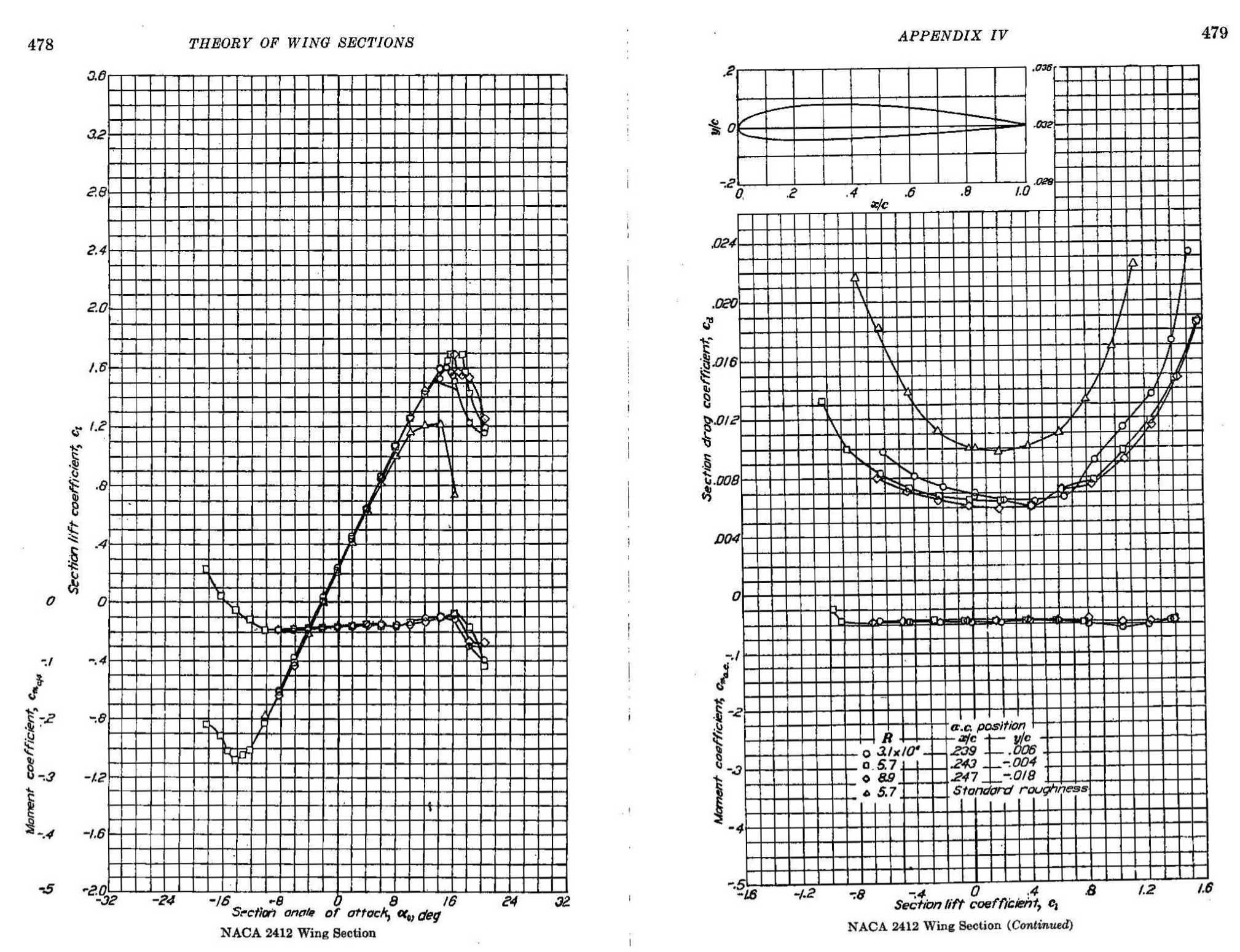
The graphs below show the aerodynamic characteristics of a NACA 2412 airfoil section directly from Abbott & Von Doenhoff, i.e., the lift coefficient , the drag coefficient , and the pitching moment coefficient about the 1/4-chord axis . Use these graphs to find for a Reynolds number of 5.7 x 10⁶ for both the smooth and rough surface cases:
- The zero-lift angle of attack, .
- The maximum lift coefficient, .
- The stall angle of attack,
 .
. - The minimum drag coefficient
 and the lift coefficient at which it occurs.
Show solution/hide solution.
For the smooth airfoil at a Reynolds number of 5.7 x 10⁶:
- The legend on the graphs shows that for a Reynolds number of 5.7 × 10⁶, the results are marked by square symbols. Referring to the left-side plot, the zero-lift angle for the smooth airfoil is approximately -2.1 °.
- The maximum lift coefficient is about 1.68 for the smooth airfoil.
- For the smooth airfoil, the corresponding stall angle of attack is about 17.6o.
- These values can be found from the right-side plot; the minimum drag coefficient for the smooth airfoil is approximately 0.06 at a lift coefficient of 0.4.
For the rough airfoil at a Reynolds number of 5.7 x 10⁶:
- The legend shows that triangular symbols mark the results in this case, so referring to the left-side plot, this zero-lift angle for the rough airfoil is unchanged at about -2.1o.
- The maximum lift coefficient is lower, at approximately 1.21, for the rough airfoil.
- The corresponding stall angle of attack is about 15.1o for the rough airfoil.
- These values can be found in the right-hand plot, where the minimum drag coefficient is higher than for the smooth airfoil and is approximately 0.098 at a lift coefficient of 0.18.
The drag curves show that an airfoil’s drag coefficient remains relatively low and reasonably constant below the onset of the stall. However, the effects of surface roughness are different when the airfoil’s leading edge is roughened up to represent the in-service degradation of a wing’s surface. Roughness causes a boundary layer to become turbulent almost immediately after it forms, resulting in higher average drag and a more rapid increase in drag as the angle of attack increases.
Lift Characteristics
At lower angles of attack below the stall, it has been noted that the lift coefficient on the airfoil section is nearly proportional to its angle of attack and the local dynamic pressure. This linear relationship is exact within the framework of linearized inviscid aerodynamic theory. The lift per unit span can be written as
(6) 
where  is called the lift-curve slope (i.e., of the slope of the lift curve in the linear part of the graph) and is measured in units per degree or radian angle of attack. It is a common mistake to assume that the value of is dimensionless, but remember, it is measured in terms of per unit of angle of attack, i.e., per degree (
 ) or per radian (
 rad). At low Mach numbers,
  per radian or 0.11 per degree.
(7) 
Remember that the preceding relationship in Eq. 7 comes under the category of linearized aerodynamics. In fact, for most airfoils, it is found that the lift coefficient varies linearly to within about 10% of that given in Eq. 7 up to an angle of about 10o to 12o, depending on the Mach number and Reynolds number, i.e., up to the point of stall.
Check Your Understanding #2 – Calculating lift coefficients
Assuming a constant lift-curve slope of 6.1 per radian angle of attack for a two-dimensional airfoil, calculate the lift coefficients at 5o, 10o and 15o angle of attack for:
- A symmetric airfoil.
- A positively cambered airfoil with a zero lift angle of attack of -1.2o.
Show solution/hide solution.
The relevant equation for the lift coefficient is
![\[ C_l = C_{l_{\alpha}} \left( \alpha - \alpha_0 \right) \]](https://eaglepubs.erau.edu/app/uploads/quicklatex/quicklatex.com-8cded43c5a6e2296e870f97cee514169_l3.svg "Rendered by QuickLaTeX.com")
The lift-curve slope  is given as 6.1 per radian angle of attack. Notice that 360
 radians so 1
 radians, i.e., = 6.1 per radian is equal to 0.1065 per degree.
 . For 5 then = 0.532, for 10 then = 1.065, and for 15 then = 1.597.
 . For 5 then = 0.660, for 10, then = 1.193, and for 15 then = 1.725.
The simplicity of the relationship in Eq. 7 is advantageous in various engineering analyses, although its limitations to airfoil operation below stall must be recognized. However, it should be noted that no simple equations can be used to represent the variation of the aerodynamic coefficients in the post-stall regime, as they vary non-linearly with the angle of attack.
Maximum Lift & Stall Types
As previously discussed, as the angle of attack increases, the adverse pressure gradient over the upper surface intensifies, thickening the boundary layer and disrupting the otherwise linear relationship between lift and angle of attack. As a critical angle is approached, flow separation occurs, and the airfoil stalls. The lift coefficient at which the airfoil stalls is called the maximum lift coefficient, denoted by .
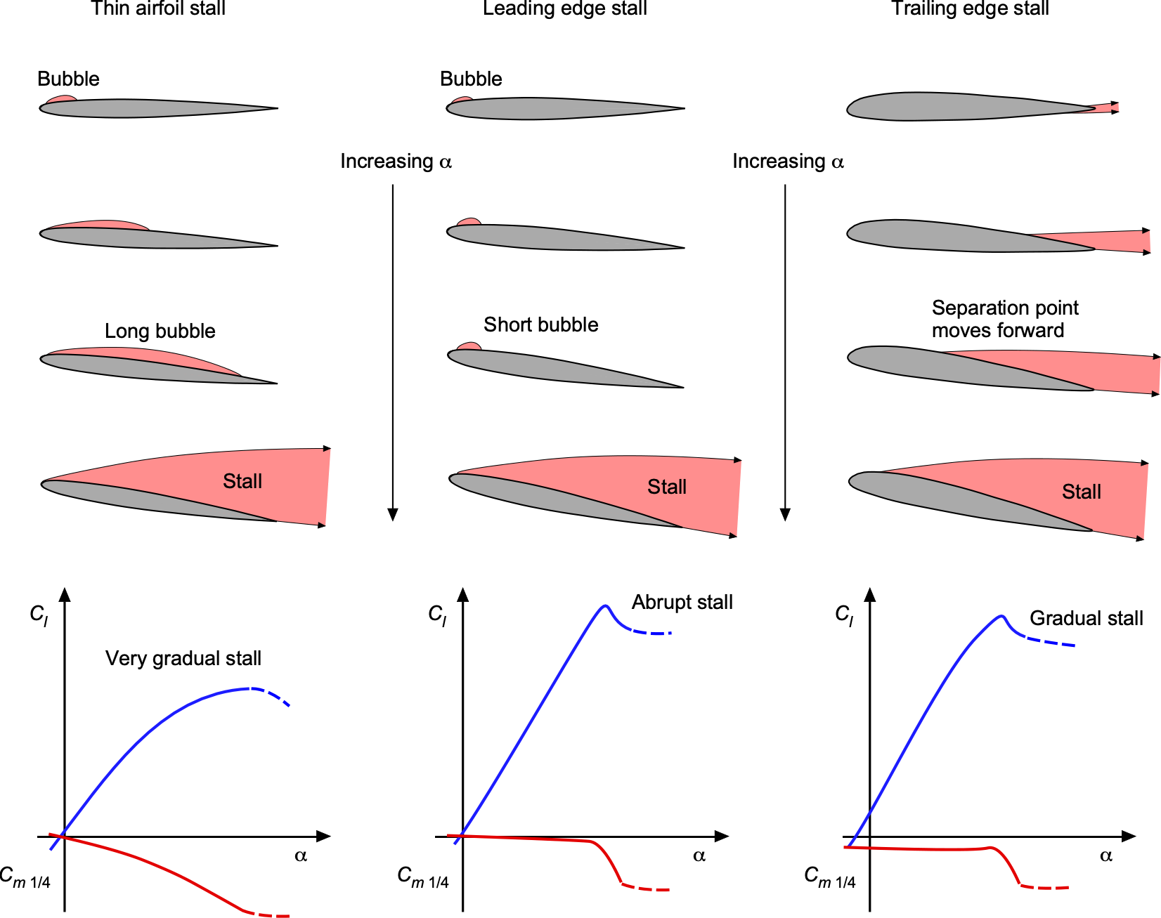
The stall process and the achievable value of will depend on both airfoil shape and its operating conditions, i.e., Reynolds and Mach numbers. Some airfoils, particularly those with greater thickness and camber, exhibit a gradual onset of stall, whereas others with sharp leading edges stall abruptly. Under subsonic flow conditions, airfoils generally fall into three primary categories of stall: thin-airfoil stall, leading-edge stall, and trailing-edge stall. These classifications are based on the location and movement of the point of flow separation on the airfoil’s upper surface, as well as its effect on lift and pitching moment.
Representative examples of the lift and moment curves illustrating the three types of stall are shown in the figure below for a NACA 63-series airfoil with varying thickness-to-chord ratios. As the name implies, thin-airfoil stall occurs on airfoils with low thickness-to-chord ratios and sharp leading edges. High adverse pressure near the nose leads to laminar separation and the formation of a long separation bubble. As the angle of attack increases, the reattachment point moves rearward until reattachment fails. The lift curve displays a gradual break, and the moment curve shows a nose-down trend at relatively low angles. In the stalled condition, the upper surface experiences nearly constant static pressure, leading to reduced lift and a significant increase in pressure drag. The center of pressure shifts aft, resulting in a more decisive nose-down pitching moment about the quarter-chord. Airfoils that exhibit thin-airfoil stall tend to produce relatively low values of .
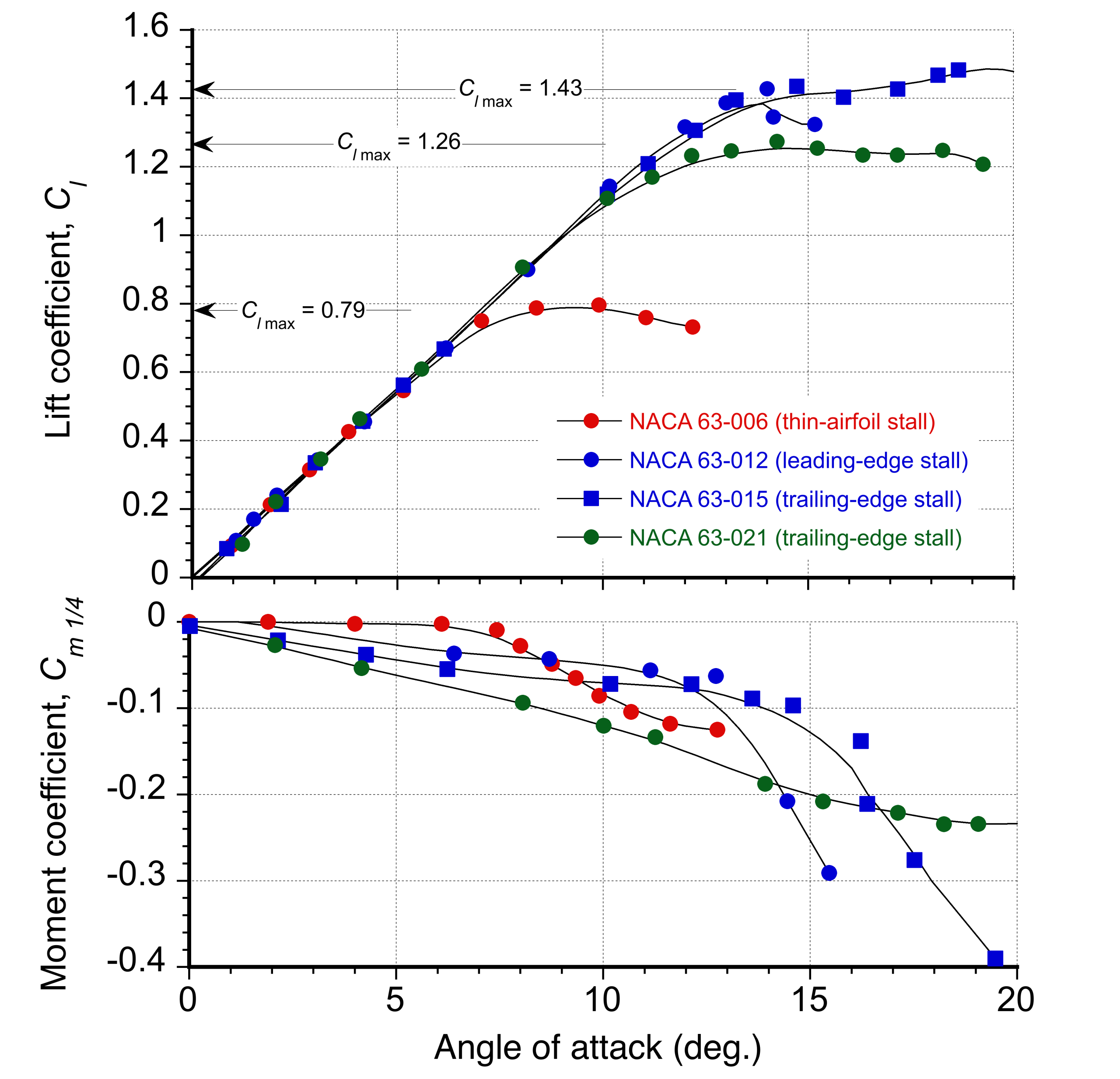
Leading-edge stall occurs on airfoils with moderate thickness and pronounced camber. A small laminar separation bubble typically forms near the leading edge of the airfoil section. As the angle of attack increases, this bubble may either burst when the boundary layer fails to reattach or the flow may undergo turbulent reseparation just downstream of the bubble. The latter is the more common mechanism at higher Reynolds numbers. Both processes lead to an abrupt stall onset, marked by a sharp loss of lift and a rapid change in pitching moment. Airfoils that exhibit leading-edge stall generally achieve the highest values of .
Trailing-edge stall is more gradual and typically occurs on thicker or more highly cambered airfoils. The turbulent boundary layer separates near the trailing edge and shifts forward as the angle of attack increases. This results in a rounded peak in the lift curve and a relatively modest nose-down change in pitching moment. Trailing-edge stall is generally less sensitive to airfoil shape and Reynolds number and tends to be more predictable. However, at higher Reynolds numbers, it can still occur abruptly and may resemble a leading-edge stall if detailed flow diagnostics are unavailable. Airfoils that exhibit trailing-edge stall generally achieve high values of . A schematic summary of the three stall mechanisms is shown in the figure below.
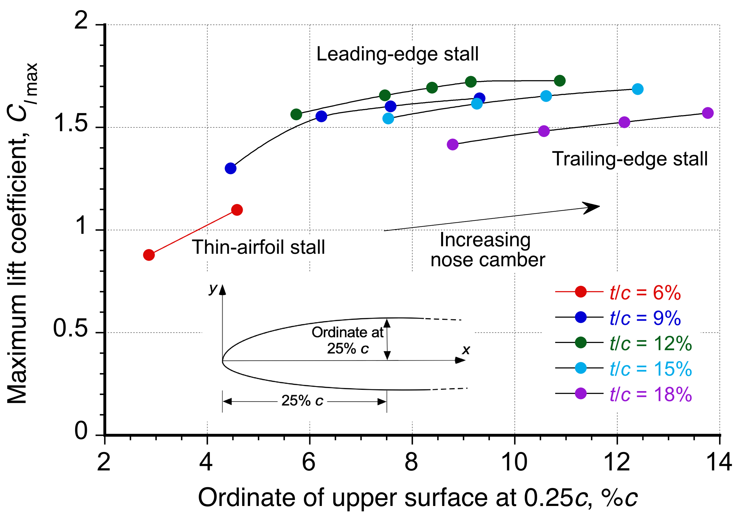
Airfoil geometry, including thickness-to-chord ratio and camber, strongly influences the maximum lift coefficient, . A summary of these effects is shown in the figure below, with the ordinate at 25% representing a combined geometric metric of the thickness-to-chord ratio,  , and camber. Increasing the of the airfoil up to about 15% generally improves the value of , although further increases yield diminishing returns unless needed for structural considerations. Forward camber increases to a point by reducing the pressure gradient at the leading edge and delaying flow separation. Cambered airfoils typically achieve higher values of than symmetric ones. However, this often comes with a more negative nose-down pitching moment, which may be a consideration in specific applications.
Effect of Flaps
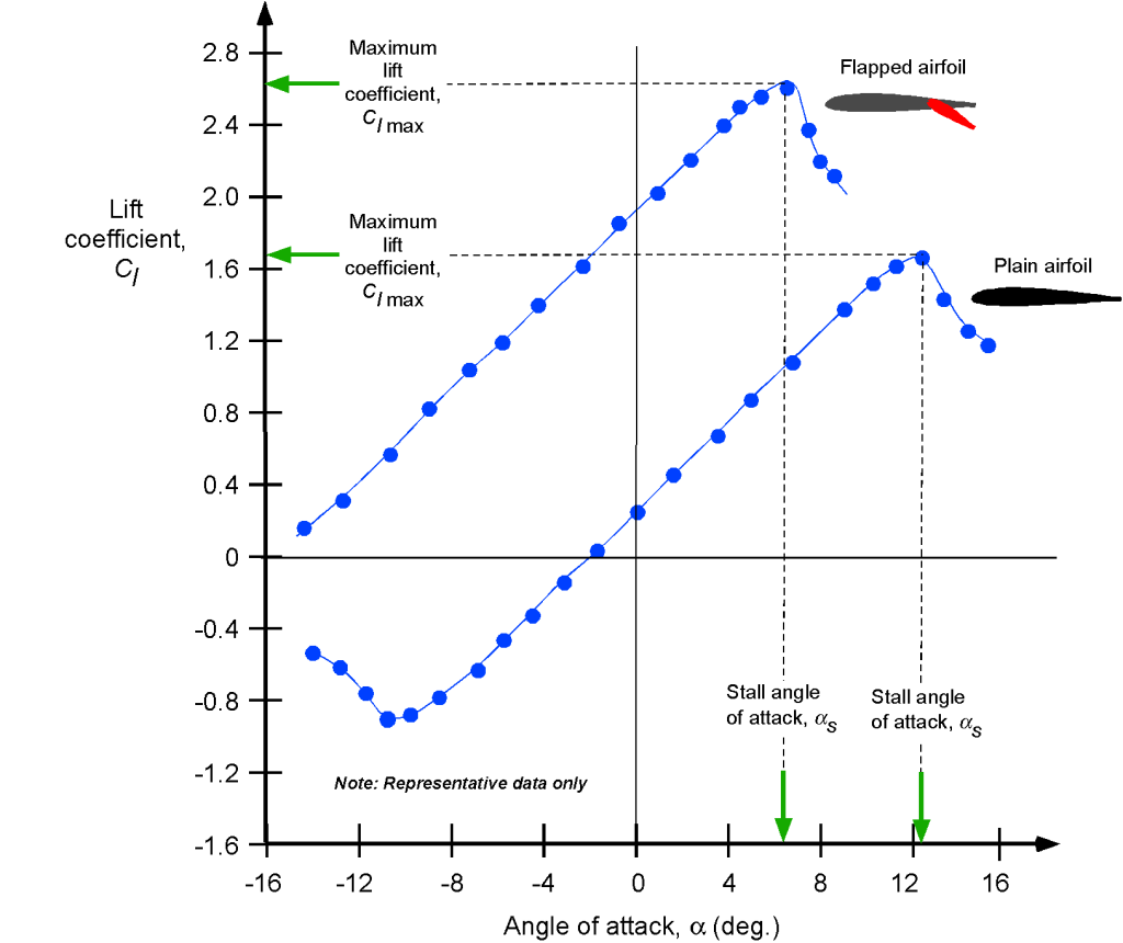
The figure below shows the effects of a flap on the lift characteristics of an airfoil. First, notice that the flap deflection introduces a form of trailing-edge camber, so the lift curve shifts to the left, giving a much lower zero lift angle of attack, changing from about -2o to nearly -16o. Second, notice the significant increase in the maximum lift coefficient from about 1.6 to 2.6 before the airfoil stalls. Such substantial increases before the onset of stall are beneficial because they will allow a wing to fly at a lower airspeed. Therefore, flaps will significantly decrease an aircraft’s takeoff and landing distances. Notice, however, that there is also a decrease in the stall angle of attack with flaps.
The increase in lift coefficient on an airfoil from a flap deflected by a small angle  (in radians) is given by
(8) 
where is the lift-curve slope of the airfoil (per radian),  is the ratio of the flap chord to the airfoil chord,
  is the flap effectiveness factor, and is the flap deflection in radians. For a simple (plain) flap, as shown in the figure above, the effectiveness factor is often approximated by
(9) 
which can be established from thin airfoil theory, so that the incremental lift coefficient becomes
(10) 
For example, for a trailing edge flap that is 25% of the chord, then = = 0.875 and  where is in radians or
  where is in degrees. Trailing edge flaps are very effective in increasing lift, with only a 10o flap deflection giving a
  of about 0.24
Further increases in the maximum lift coefficient may be achievable with different types of flaps, such as slotted, Fowler, or double- or triple-slotted. Typical values of for common flap types are:
(11) ![\begin{equation*} \begin{aligned} \text{\small Plain flap: } \eta_f &\approx 1 - \dfrac{c_f}{2c} \\[4pt] \text{\small Split flap: } \eta_f &\approx 0.8 \\[6pt] \text{\small Slotted flap: } \eta_f &\approx 1.2 \text{ to } 1.3 \\[6pt] \text{\small Fowler flap: } \eta_f &\approx 1.3 \text{ to } 1.4 \end{aligned} \end{equation*}](https://eaglepubs.erau.edu/app/uploads/quicklatex/quicklatex.com-cdb9dd1e1db4e6114dccd1fd35f92058_l3.svg "Rendered by QuickLaTeX.com")
In conjunction with leading-edge slats, significant stall speed reductions can be achieved with larger airliner types of airplanes. For an airplane, however, the penalties for using more complicated flap systems include increased airframe weight, higher costs, and increased maintenance.
Drag Characteristics
The variation in drag with angle of attack and/or lift coefficient is of great interest due to its significant effects on aircraft performance. Specifically, drag generally reduces the aircraft’s performance. Some representative results are shown in the figure below, illustrating the drag coefficient versus the lift coefficient for both a conventional airfoil (in this case, the NACA 23012) and a so-called “laminar flow” airfoil (a NACA 63-series airfoil). The variation of the drag coefficient for the NACA 23012 airfoil is typical. The drag remains low until the angle of attack and the corresponding lift coefficient increase to the point at which significant boundary-layer thickening occurs. Then, the drag grows rapidly when a stall occurs.
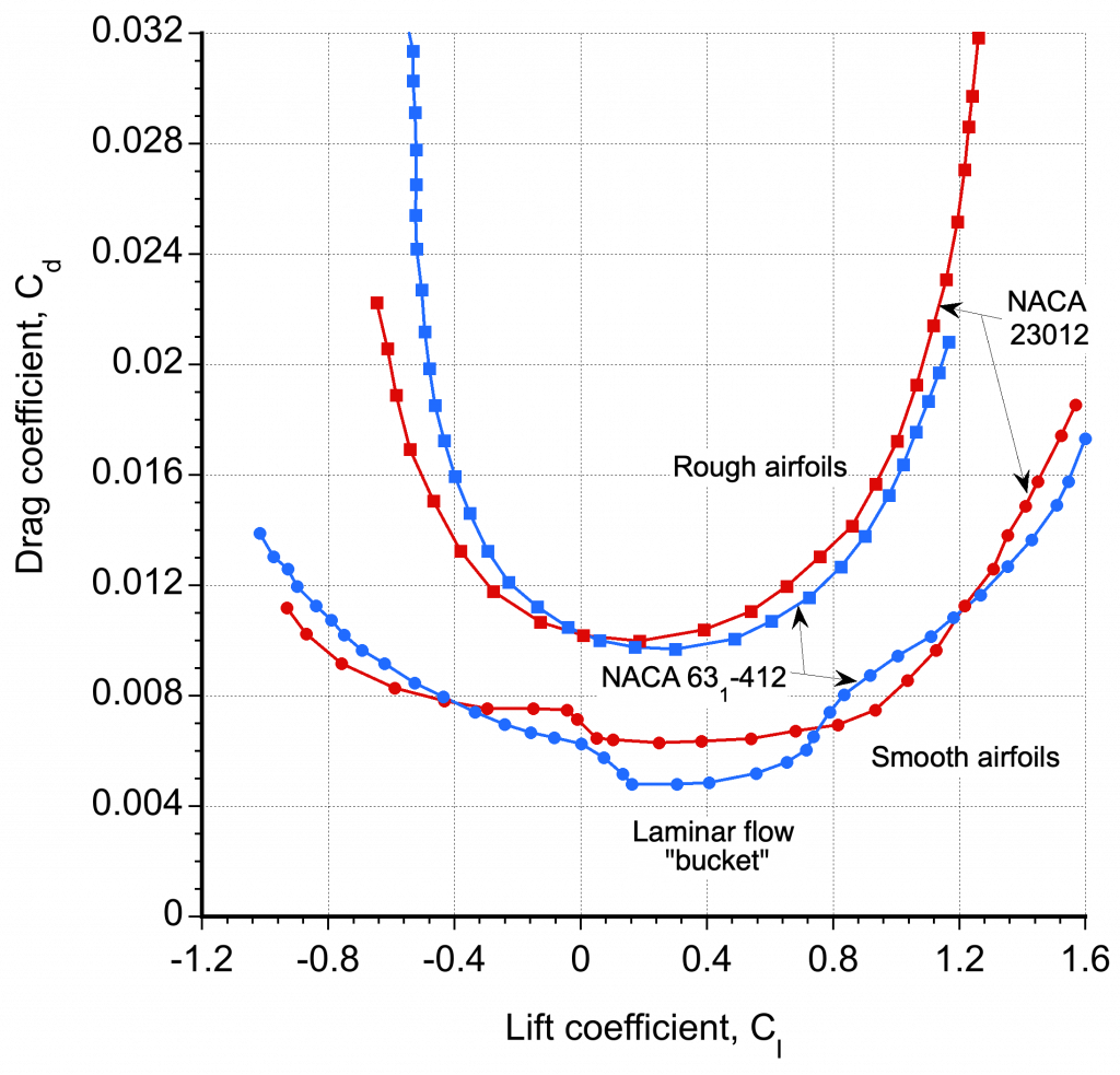
Notice that the effects of surface roughness substantially increase the values of drag. Although these results are from wind tunnel tests, the effects of roughness can simulate the typical “in-service” abrasion of the leading edges of wings compared to when they were new from the factory (and thus initially smoother). The effects of roughness are significant. In airplane design, it is necessary to account for surface roughness to avoid overestimating the aircraft’s potential performance by assuming a perfectly smooth airfoil, which is unlikely to be achievable in practical flight operations.
In the lower angle of attack regime, the drag coefficient on an airfoil can be represented by the equation
(12) 
where ,  , and
, and  are empirically derived coefficients (obtained through curve fitting) to drag measurements for a specific airfoil at a given Mach number and Reynolds number. Because in the linear regime then
  , then it is also possible to write that
(13) 
Again, it is essential to recognize that the preceding equation can only represent airfoil characteristics below stall; it is invalid in the presence of significant flow separation or the stalled flow regime. In the case of a symmetric airfoil (where  then and
  will be zero.
The figure above also shows results for a NACA 63-series laminar-flow airfoil, a design that maximizes the extent of the laminar boundary layer along the leading edge, thereby reducing skin friction drag. These airfoils, with very smooth surfaces, tend to produce low-drag “buckets” where the drag is relatively lower, but typically only over a limited range when the airfoil operates at low angles of attack and low lift coefficients.
The geometric shapes of these laminar flow airfoils tend to have a point of maximum thickness much closer to the 1/2-chord than more conventional airfoils, which will have a maximum thickness nearer to the 1/4-chord, as shown in the figure below. This geometric feature produces a favorable pressure gradient over a larger portion of the leading edge, thereby encouraging the boundary layer to remain laminar for a longer downstream distance. The downside is that such airfoils typically produce lower maximum lift coefficients, i.e., stall occurs at lower angles of attack.

The previous discussion also suggests that surface roughness encourages turbulent mixing, quickly destroying the laminar boundary layer. The resulting increase in skin friction drag makes the airfoil perform comparably (or sometimes worse) than a conventional airfoil. This latter reason is why laminar-flow airfoil sections are challenging to use effectively in practice: some surface roughness on the wing is inevitable.
However, such airfoils have seen better success for us on the smooth, almost glass-like wings of sailplanes, although the wings must be polished and kept completely clean and free of debris for laminar flow to prevail. Nevertheless, obtaining an extensive laminar flow region on an airfoil can significantly reduce its drag, at least over a specific range of angles of attack and lift coefficients. Unfortunately, a practical and robust means of achieving extensive laminar flow regions on an airplane wing remains a research challenge, although specific surface coatings are helpful.
Drag Polars
Types of graphical presentations of versus or versus are often referred to as a “drag polar” or simply a “polar,” as shown in the figure below. Polars are a helpful way to present airfoil section characteristics because results for different operating conditions (e.g., Reynolds or Mach numbers) or different airfoils can be readily compared and contrasted on a single plot.
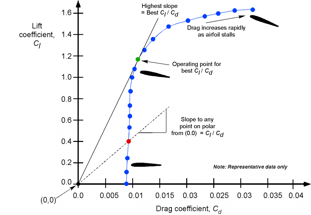
One advantage of the versus form of the presentation shown above is that the slope of a straight line running from the origin (0, 0) of the graph to any point on the polar is a measure of the lift-to-drag ratio and hence is a quantitative measure of the airfoil’s aerodynamic efficiency. Notice that the tangent to the polar gives the highest slope. This point represents the best lift-to-drag ratio, i.e., the operating conditions at which the airfoil achieves its highest aerodynamic efficiency. Notice also that there is only one angle of attack and operating lift coefficient for best efficiency, which depends on the particular airfoil shape, its operating Reynolds number, and Mach number.
Effects of Reynolds Number
The classic NACA airfoil measurements also indicate some effect of the Reynolds number, at least over a limited range, but all the results are above one million. Remember that for an airfoil, the Reynolds number will be based on the chord, , so
(14) 
The “c” subscript on the Reynolds number is often dropped, so  is used instead. Flight vehicles typically experience higher chord Reynolds numbers, usually as high as
  , or approximately one hundred million. Notice that the Reynolds number is often quoted in millions. For example, for
  , the value of the Reynolds number is usually referred to as “a Reynolds number of three million.”
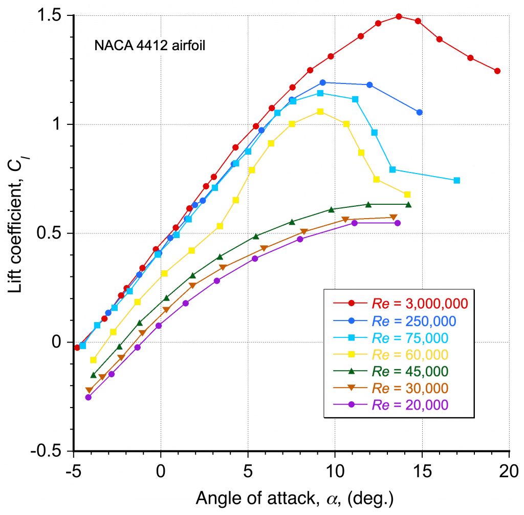
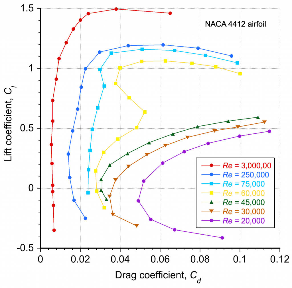
As the Reynolds number decreases below one million ( ) and viscosity begins to outweigh inertia in the flow, the lift and drag characteristics undergo profound changes. The aerodynamic characteristics of airfoils at lower chord Reynolds numbers are important because they affect the performance of many smaller-scale flight vehicles, such as UAVs and drones, which often have chord-based Reynolds numbers well below a million. The data in the figure below show the profound effects of operating airfoils at lower Reynolds numbers, ranging from 20,000 to 3,000,000 (three million).
 with the angle of attack for a NACA 4412 airfoil when operating at different Reynolds numbers.
At the highest Reynolds number of  , the lift coefficient varies almost linearly with the angle of attack, and the drag is nominally constant, which is typical of airfoil behavior at higher Reynolds numbers, as previously discussed. However, as the Reynolds number decreases below a million, the lift and drag curves become significantly more rounded and eventually become nonlinear for variations in the angle of attack. Indeed, these effects start to become pronounced even at Reynolds numbers of 500,000.
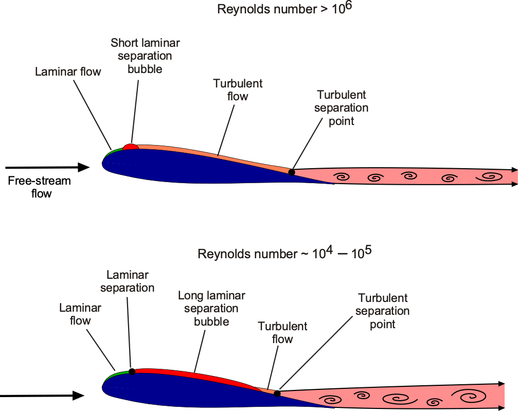
This latter behavior directly results from the relatively thicker boundary layers on the airfoil surfaces at these lower Reynolds numbers. Furthermore, the development of a long laminar separation bubble (LSB) on the airfoil is often a source of these nonlinear characteristics, as shown in the figure below. In these cases, the airfoil’s lift (and drag) behavior becomes much more challenging to generalize as a function of the angle of attack, i.e., the relationship in Eq. 7, for example, is no longer applicable. In general, at lower Reynolds numbers where  , the lower momentum in the boundary layer flow leads to thicker boundary layers and higher drag. Naturally, this type of flow physics presents challenges in measuring lift and drag in a wind tunnel, where careful ensemble averaging is required.
The corresponding drag polar for these conditions is shown in the plot below, providing another helpful way to summarize the effects of Reynolds number on the aerodynamic characteristics. Notice again the profound effects of reducing the Reynolds number below 500,000, which deleteriously affect the lift-to-drag ratio, especially below 50,000. For extremely low Reynolds numbers of less than  , lift-to-drag ratios of less than 5 are expected, at least with “conventional” airfoil sections.
At this point, a natural question arises: do better airfoil shapes exist for use at low Reynolds numbers? The answer is yes, but identifying optimal shapes requires a detailed understanding of boundary layer behavior under these conditions. Michael Selig provides an in-depth discussion of these aerodynamic issues in his lecture notes on low-Reynolds-number designs. More recently, the use of CFD has enabled confident prediction of airfoil performance at low Reynolds numbers. Because the aerodynamic forces and moments involved are small, experimental measurements at these scales can be complex and prone to error. CFD therefore plays a valuable role in supplementing wind-tunnel data and revealing systematic trends that may not be readily observed experimentally.
As shown in the figure below, one notable effect is the sharp increase in drag at lower lift coefficients as the Reynolds number decreases, a trend previously discussed. Another observation is the historical performance of legacy airfoils such as the NACA 0012 and the Clark Y. The latter, designed by Virginius E. Clark in 1922, was derived from the Göttingen 398 airfoil. The Clark Y has a maximum thickness-to-chord ratio of 11.7% and is flat on its lower surface aft of 30% chord. While it offers reasonable aerodynamic performance, it is rarely used in modern designs. Contemporary airfoils exhibit much greater sensitivity to Reynolds number than older plate-type shapes. For example, the maximum lift coefficient of a simple 6% cambered plate increases from approximately 1.15 at a Reynolds number of 200,000 to about 1.32 at a Reynolds number of 10 .
.
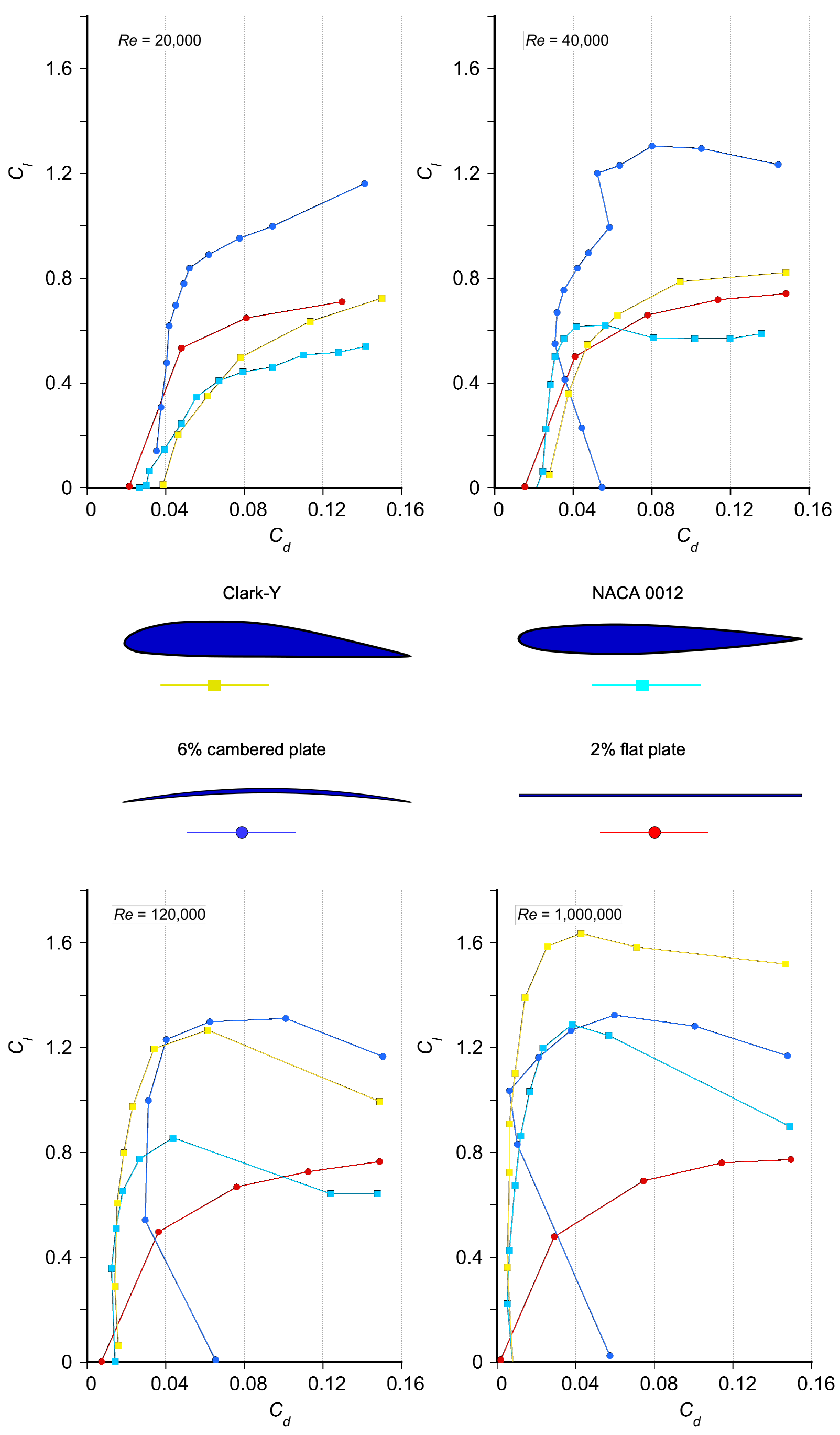
However, notice that the peak lift coefficient of the flat plate is virtually unchanged. Over the same Reynolds number range, the peak lift coefficient more than doubles for the NACA 0012 and Clark-Y. Clearly, at the lowest Reynolds numbers, the thinner airfoils outperform the thicker ones in terms of aerodynamic efficiency, contrary to conventional wisdom. For example, the cambered plate exhibits a maximum lift-to-drag ratio of approximately 23 at a lift coefficient of 0.8. In contrast, the Clark-Y has a lift-to-drag ratio of about half that of the Clark-Y at a significantly lower lift coefficient.
Effects of Mach Number
During the 1950s, the field of aeronautics continued to advance quickly, and with the advent of the turbojet engine, airplanes began to fly much faster. Soon, the effects of compressibility on their performance became increasingly apparent, including higher drag and phenomena such as wave drag, shock-induced flow separation, and buffeting from flow separation. The significant increase in drag and buffeting on an aircraft as it approached the speed of sound (Mach 1) was initially referred to as the sound barrier. Still, it is now known that there is no intrinsic aerodynamic barrier to attaining supersonic flight if sufficient thrust is available to overcome the associated aerodynamic drag.
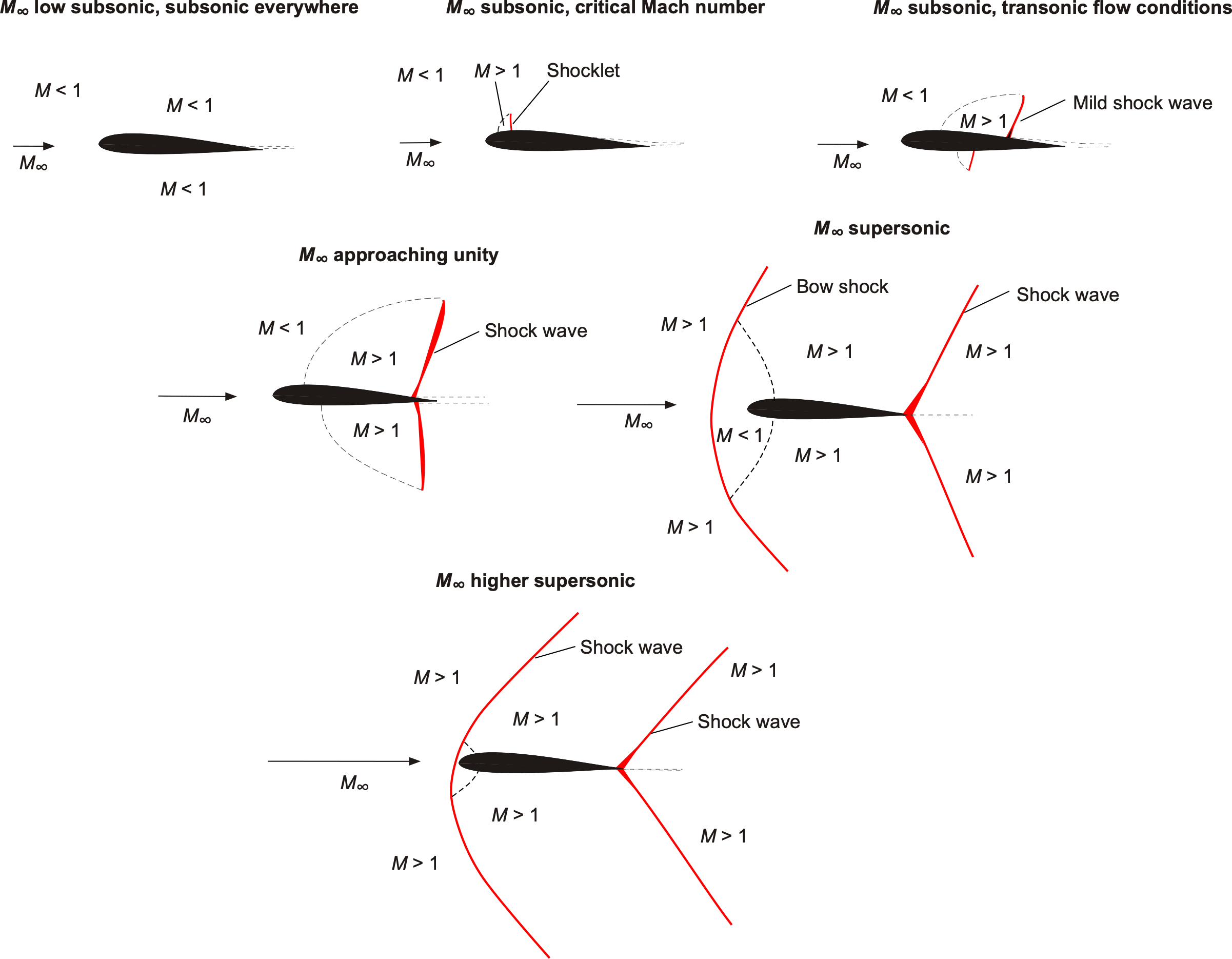
A significant amount of research has been devoted to understanding the effects of compressibility on airfoils and wings, as well as to developing suitable airfoil sections and wing shapes that mitigate its adverse effects at higher flight Mach numbers. The figure below shows schlieren images of the compressible flow around a 10% thickness-to-chord ratio symmetric airfoil set at an angle of attack of 2o in the wind tunnel. The refraction of light rays produces the schlieren effect as they pass through the regions of different flow densities. (Note: The lower dark vertical line in these images is a model support in the optical path but not in the flow.) Furthermore, it is worth noting that these circular images arise because the schlieren flow visualization system utilizes spherical or parabolic concave mirrors.
This sequence of images shows what happens to the flow about the airfoil as the freestream Mach number  (notice that
  is used to denote the freestream Mach number in the captions to these images) is gradually increased from a subsonic flow just below the critical Mach number through transonic conditions and until the flow becomes supersonic. The differences delineate the developments of the shock waves and other compressible flow patterns; the shock waves are the darker zones produced by the schlieren effects.
No strong shock waves appear on the airfoil at = 0.7. Nevertheless, a close inspection of the image reveals a small, dark line near the 25% chord, indicating a weak shock wave and suggesting that the critical Mach number,  , is being reached, i.e., the flow around the airfoil becomes locally supersonic. By = 0.75, a series of small shocklets (which are mild shock waves) can be seen between 10% and 30% of the chord, confirming the existence of a supersonic pocket, and by = 0.775, a weak shock wave has formed. However, no shocks have yet formed on the lower surface.
By = 0.82, a more substantial shock wave has formed on the upper surface and moved aft on the chord, and by = 0.84, a shock develops on the lower surface almost directly below the one on the upper surface. In addition, there is clear evidence of boundary layer thickening at the bottom of the upper shock at the airfoil’s surface, resulting from the adverse pressure gradient produced there (see also the pressure distributions about airfoils discussed later in this chapter). Recall that an adverse pressure gradient is one in which the pressure increases with downstream distance, thereby slowing or retarding the flow’s development.
At = 0.88, both the upper and lower surface shock waves continue to grow in strength. The upper-surface shock bifurcates at the airfoil surface as it interacts with the boundary layer. Flow visualization suggests that the downstream boundary layer is now relatively thick. At = 0.90, the boundary layer has separated downstream of the shock on the upper surface, a phenomenon known as shock wave-induced flow separation, commonly referred to as shock-induced separation. By = 0.95, both shocks have reached the trailing edge and become significantly bifurcated from their interaction with the relatively thick boundary layer. After that, the flow becomes entirely supersonic. A summary of the preceding observations is presented below as a schematic for clarity.
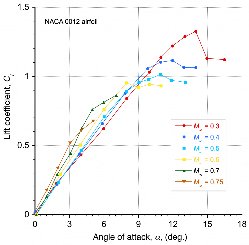
While the preceding flow visualization images are interesting and valuable, the resulting forces and moments on the airfoil are also important. The effects of the Mach number and, hence, the compressibility of the flow on the lift curve are shown in the figure below. Typically, flow with a Mach number lower than 0.3 is considered incompressible, and an airfoil will have a lift-curve slope of about  per radian or 0.11 per degree. Nevertheless, it can be seen that the lift-curve slope increases rapidly at higher Mach numbers because of the effects of compressibility. Notice also that the airfoil’s maximum lift decreases as the Mach number increases. As the Mach number approaches the critical Mach number and the onset of the transonic region (approximately 0.7), the attainable maximum lift coefficient without producing flow separation and stall is seen to be relatively low.
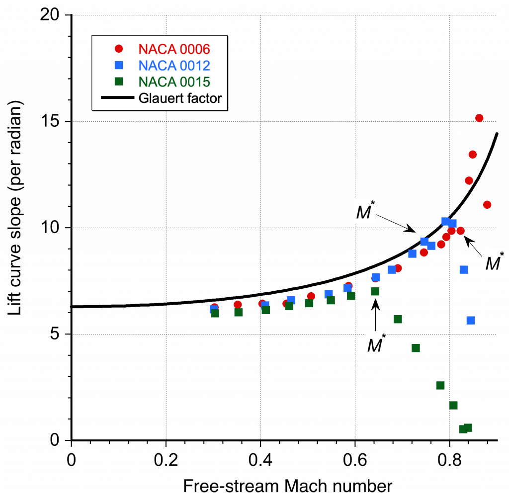
The theoretical relationship representing this latter behavior on the lift-curve slope is called the Glauert rule, summarized in the figure below and compared with measurements from three NACA symmetric airfoil sections. The Glauert rule states that the lift-curve slope increases according to
(15) 
which is theoretically exact for a thin airfoil in subsonic flow. A generalization of this result is to correct the low Mach number value of the lift coefficient using
(16) 
These latter relationships hold for many airfoils of practical interest. Still, there are exceptions, especially for airfoils with higher thickness-to-chord ratios or significant nose camber. The validity of the Glauert rule generally extends up to the critical Mach number for the airfoil section, , i.e., the onset of supercritical flow.
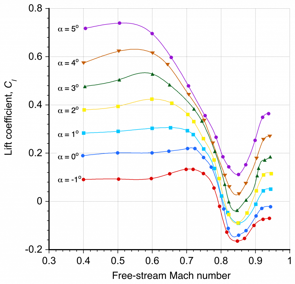
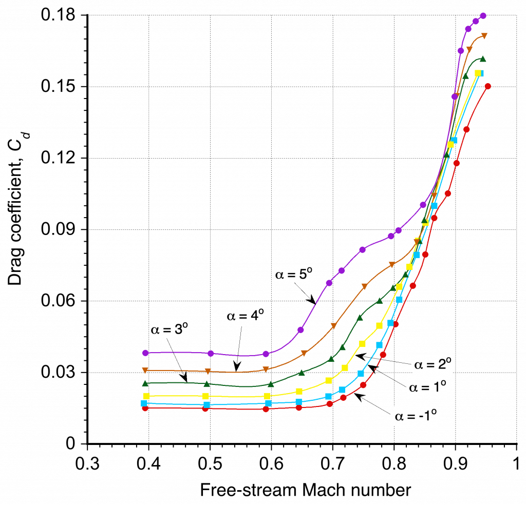
Further examples of the effects of compressibility on the lift and drag characteristics of an airfoil are shown in the two figures below. Notice the increase in the lift coefficient for a given angle of attack with increasing Mach number, but to a point. This outcome means that the lift is higher for a given dynamic pressure. However, it is also worth noting that for a given angle of attack, reductions in lift coefficient and increases in drag coefficient occur when the Mach number exceeds a critical value; i.e., the stall angle of attack of the airfoil decreases as the Mach number increases.
What airfoil section should be used?
Selecting an airfoil for a specific purpose is a deliberate process that requires careful consideration and often considerable time. If done correctly, the process will involve both computational methods (for iterative design) and wind tunnel testing (to verify the final airfoil), but this is only ideal. Today, many airfoils can be confidently designed solely with computational methods, though this carries some risk. Airfoils tend to be “point” designs, so they often perform optimally only at one specific combination of angle of attack (or lift coefficient), Reynolds number, and Mach number. Trade studies will inevitably focus on the minimum drag coefficient, the maximum lift-to-drag ratio, the lift-to-drag ratio at the design point, the maximum lift coefficient, and the overall pitching moment behavior. The most important aircraft performance criteria will inevitably define the most suitable airfoil shape. However, the success of the airfoil section also depends on its performance in off-design conditions. It is generally advisable to allow sufficient robustness in the design to ensure acceptable operation throughout the operational flight envelope. The consideration of maneuvers and gusts may also dictate the aerodynamic margins that need to be built into the airfoil design to prevent premature stall or other adverse aerodynamic behavior.
Pitching Moments
The behavior of the pitching moment on an airfoil is also important. It is always convenient to place the integrated forces at some convenient point on the airfoil, but the question is: At what point? The answer is that the forces can be located at any point if the corresponding moment about that same point is also defined.
In many aerodynamic applications, the 1/4-chord point is used as a reference point, i.e.,  . The 1/4-chord has theoretical significance, as it is the aerodynamic center for a thin airfoil in an incompressible flow. However, even if another reference point was selected, converting from one to another is easy because it just requires applying the rules of statics, as shown in the figure below.
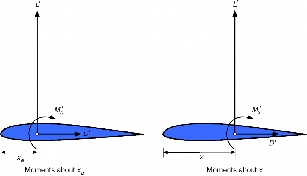
For example, assume the lift force (or normal force) and pitching moment per unit span are known at a point at a distance  from the leading edge of the airfoil, and it is desired to find the pitching moment about another point, say at a distance
  behind the leading edge. Taking moments about the leading edge in each case gives
(17) 
Converting to coefficient form by dividing by  gives
gives
(18) 
where the overbar means that the length scale has now been non-dimensionalized with respect to the chord, i.e.,  . For example, if the known pitching moment is about the leading edge,
  , then
 and the above equation becomes
(19) 
Center of Pressure & Aerodynamic Center
The concepts of center of pressure and aerodynamic center are used routinely in aerodynamic analysis, and it is essential to understand their differences. They are frequently confused in practice, though they are distinctly different.
Center of Pressure
By definition, the center of pressure is a point about which the moments are zero, i.e., a point where the resultant forces can be assumed to act. The principle is illustrated in the figure below, where the center of pressure location,  , effectively serves as the balance point (or fulcrum) of the aerodynamic forces.
The center and pressure (as well as the aerodynamic center) can be determined if the lift and moment coefficients are known about any other point, the 1/4-chord often being used as a reference point, i.e., the values of and are available. The best way for the reader to understand the process is to work through an example using actual airfoil measurements, which are provided in the table below for a NACA 0012 (symmetric) airfoil.
| Angle of attack | Lift coefficient | Drag coefficient | Moment coefficient |
|---|---|---|---|
| 0 | 0 | 0.00662 | 0 |
| 1 | 0.1096 | 0.0067 | 0.0006 |
| 2 | 0.2182 | 0.00693 | 0.0013 |
| 3 | 0.3254 | 0.00736 | 0.0024 |
| 4 | 0.4309 | 0.008 | 0.0038 |
| 5 | 0.5365 | 0.00881 | 0.0054 |
| 6 | 0.6509 | 0.00976 | 0.0057 |
| 7 | 0.7743 | 0.01085 | 0.0057 |
| 8 | 0.9006 | 0.01203 | 0.0041 |
| 9 | 0.9957 | 0.01328 | 0.0046 |
| 10 | 1.0836 | 0.01466 | 0.0046 |
| 11 | 1.1729 | 0.01627 | 0.0079 |
| 12 | 1.2585 | 0.01817 | 0.0113 |
| 13 | 1.3343 | 0.02057 | 0.0157 |
| 14 | 1.3928 | 0.02328 | 0.0221 |
| 15 | 1.4322 | 0.02739 | 0.0284 |
| 16 | 1.4511 | 0.0345 | 0.0315 |
| 17 | 1.4508 | 0.04615 | 0.0287 |
| 18 | 1.4004 | 0.06732 | 0.0186 |
| 19 | 1.2739 | 0.10324 | 0.0001 |
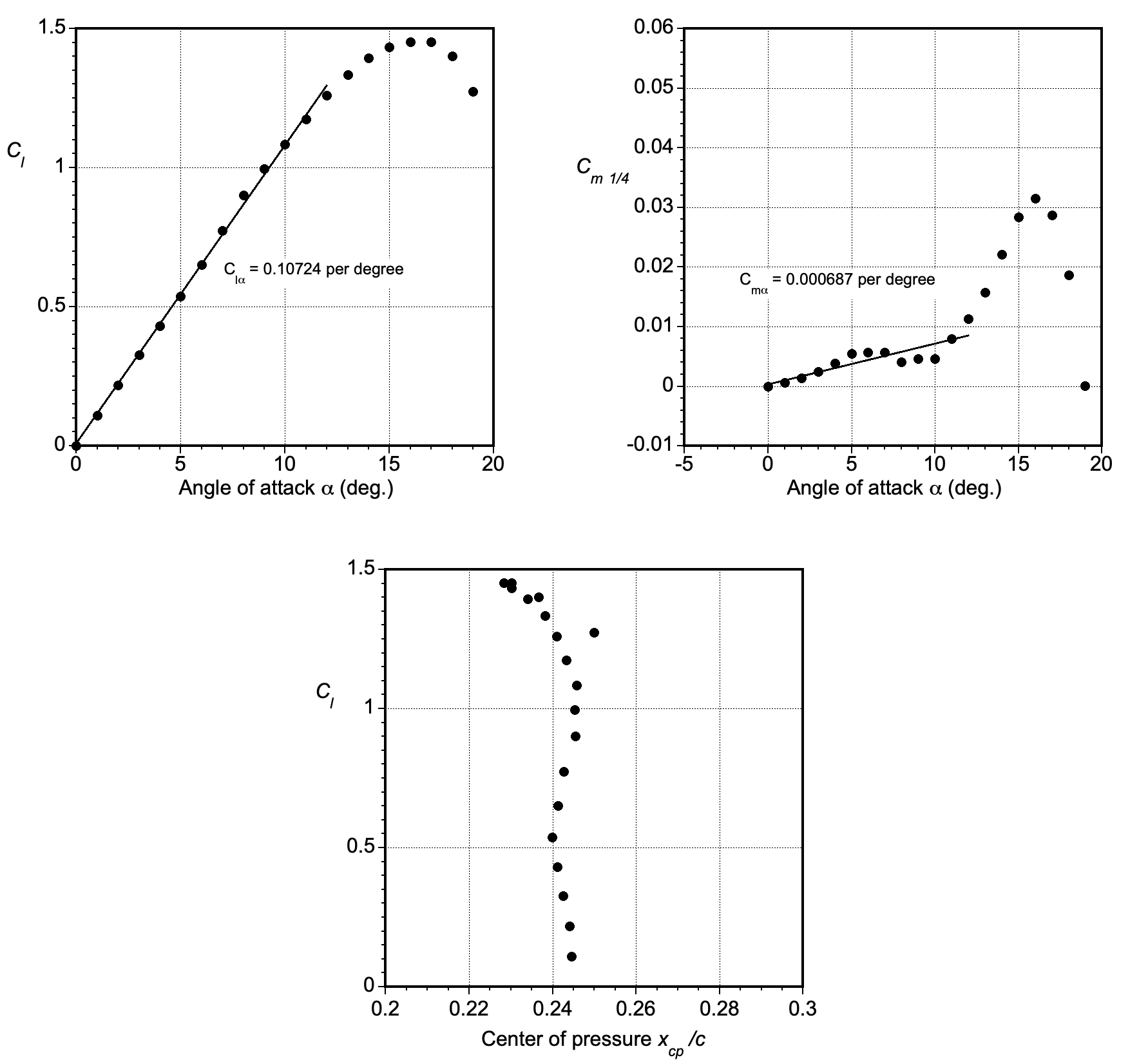
These data are shown in the figure below in the form of lift coefficient, , versus angle of attack, , the pitching moment coefficient about the 1/4-chord versus , and the center of pressure location versus . The slope of the lift curve (i.e., the lift-curve slope, ) and the slope of the moment curve (i.e., .
To find the position of the center of pressure, say downstream of the leading edge (LE) where the pitching moment would be zero, this is done by first taking moments about the leading edge, i.e., the application of statics gives
(20) 
In coefficient form (divide by  ), this result becomes
(21) 
so that the center of pressure (as a fraction of the chord) is given by
(22) 
For most airfoils with positive camber, the value of  is negative, indicating that the center of pressure is generally located behind the 1/4-chord. In particular, notice that the center of pressure will be a function of the lift coefficient (and hence also the angle of attack), so it is not a fixed point, as shown in the above figure. Because the center of pressure is a moving point and may not even be located on the airfoil’s chord, the concept of center of pressure is only sometimes a convenient one to use in aerodynamics. Hence, the center of pressure to resolve the forces and moments is used sparingly in practice, even though the pitching moment here is zero by definition.
Aerodynamic Center
By definition, the aerodynamic center is a point where the moment is constant and independent of the angle of attack. The procedure for finding the aerodynamic center, similar to that for the center of pressure, requires values of the lift and moment coefficients at any point, such as a distance from the leading edge.
If the aerodynamic center is at a distance  behind the leading edge, then the application of statics (as explained previously) gives
(23) 
The objective is to find the location of such that the value of the pitching moment at that point is constant. Differentiating the above equation with respect to  gives
gives
(24) 
The value of  can be obtained by using
(25) 
Therefore, to calculate the aerodynamic center location, the slope of the lift curve (in the linear range) and the slope of the moment curve (also in the linear range) are needed. Remember that the linear range corresponds to conditions where the flow is fully attached to the airfoil surface. This process involves finding the slopes of the best straight line fits to the values of versus and then versus in the linear range (attached flow).
Following on with the previous example, a least-squares fit to the measurements below the stall gives
(26) 
and
(27) 
Therefore, because the 1/4-chord is being used as a moment reference, the aerodynamic center, in this case, is
given by
(28) 
It can be seen that, for the particular airfoil used here, the aerodynamic center is located at 24.25% chord. The location of the aerodynamic center depends on the airfoil section and the Mach number at which it operates. Because the value of the lift-curve slope is always positive, the slope of the moment curve defines the sign of the position of the aerodynamic center relative to the 1/4-chord. Therefore, if this slope is positive, the aerodynamic center is located ahead of the 1/4-chord; if it is negative, the aerodynamic center is located behind the 1/4-chord. For thin airfoils, the value of is almost constant, so the aerodynamic center is generally always close to 1/4-chord at low freestream Mach numbers.
It can be concluded that the advantage of using the aerodynamic center to resolve the forces and moments is convenience. It is a fixed point that remains unchanged with the angle of attack. However, determining the aerodynamic center location requires more effort, as the slopes of the lift and moment curves must be calculated.
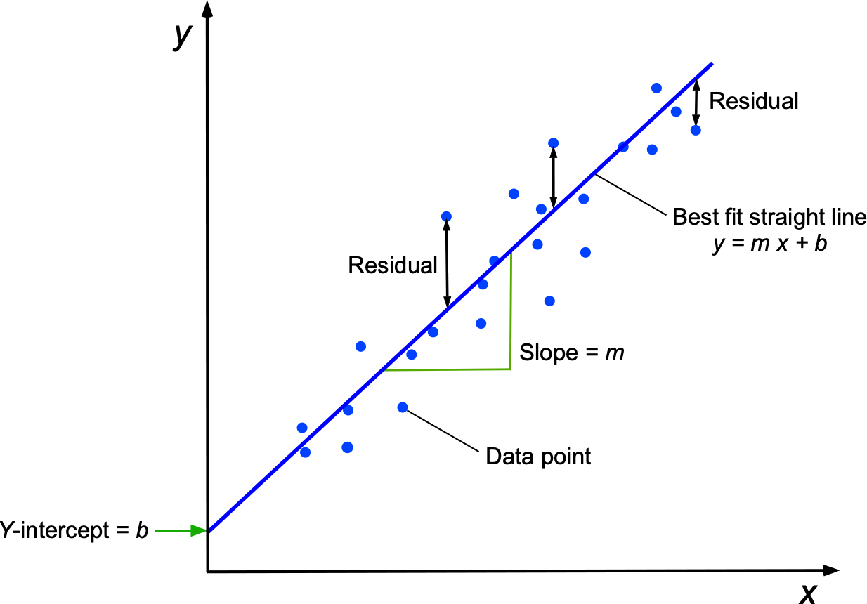
What is a least-squares linear fit?
The linear least-squares method is a numerical method for finding a straight line that best fits the trends in a given data set. The main objective is to reduce as much as possible the sum of the squares of the differences or residuals between the fitted straight line and all of the data points, as shown in the figure below.
It can be assumed that the given data points are  ,
,  ,
,  , ….,
, ….,  , where
  is the number of data points. A straight line is
  , where
  is the slope, and
  is the intercept on the
  axis. The formulas to calculate the slope and intercept of the best straight-line fit are given by
![\[ m = \frac{N \sum x y - \sum x \sum y}{N \sum x^2 - (\sum x)^2} \]](https://eaglepubs.erau.edu/app/uploads/quicklatex/quicklatex.com-12d276a13c8333eac5b222e38e8ec47c_l3.svg "Rendered by QuickLaTeX.com")
and
![\[ b = \frac{\sum y - m \sum x}{N} \]](https://eaglepubs.erau.edu/app/uploads/quicklatex/quicklatex.com-94f2bf9f151b8cd49cf9c692ecbbe424_l3.svg "Rendered by QuickLaTeX.com")
The process can also be performed in MATLAB by using the polyfit function.
Pressure & Shear Stress Coefficients
Pressure coefficients (i.e., non-dimensional pressures) are commonly used to present pressure distributions around body shapes and airfoil sections. The pressure coefficient,  , is defined as
(29) 
where  is the local static pressure and
  is the freestream static pressure. Again, notice the use of freestream dynamic pressure as a reference pressure.
Suppose the local pressure equals the freestream static pressure , then  . If the local pressure is less than the freestream static pressure , then
  . At a stagnation point (where the flow velocity is brought to zero), then
  , at least if the flow is assumed incompressible and the Bernoulli equation is being applied.
The shear stress or local skin friction coefficient is defined as
(30) 
where  is the boundary layer shear stress, which is proportional to the velocity gradient at the surface.
The total skin friction coefficient, denoted by  , is obtained by integrating the local skin friction coefficient over the surface. For example, if the surface exposed to the flow has a length , then the total shear stress coefficient is
(31) 
If two surfaces are exposed to the flow, such as the upper (u) and lower (l) surfaces of an airfoil, then the total skin friction coefficient would be equivalent to the skin friction drag coefficient, i.e.,
(32) 
Of course, these principles can be applied to any body shape and extended to three dimensions.
Integration of Pressures & Shear Stresses
Calculating or measuring pressure distributions over body shapes, such as on airfoil sections, is possible. The integration process around the body contour can then be used to determine quantities such as lift, drag, and pitching moment coefficients. The pressure values are typically two orders of magnitude greater than the shear stress, so adequate results for the lift can often (but not always) be obtained by considering only the pressures. However, for drag, shear stress must be accounted for, as it is the dominant contributor at low angles of attack.
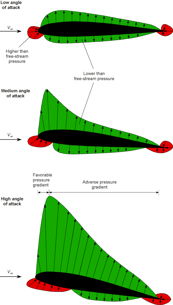
The pressure distributions around airfoil sections are non-uniform, with higher and lower pressure regions relative to ambient pressure, typical variations being shown in the figure below. While pressure is a scalar, in this presentation, the local pressure, , is plotted as a vector directed perpendicular to the local surface slope of the airfoil, i.e., in terms of  where
where  is the unit normal vector. The green zones represent lower-than-ambient pressure, and the red zones are higher-than-ambient pressure. Airfoil sections also produce substantial pressure gradients, especially near the leading edge at higher angles of attack. Therefore, the challenge is to determine the integrated quantities, which requires knowledge of the pressures and their detailed distributions.
The principle behind the integration process to find the lift can be explained with reference to the figure below. On the upper surface, the per unit span force components acting on an elemental area of width  are
are
(33) ![\begin{eqnarray*} dN'_u & = & (p_u \cos \theta_u - \tau_u \sin \theta_u ) ds_u \\[10pt] dA'_u & = & (p_u \sin \theta_u + \tau_u \cos \theta_u ) ds_u \end{eqnarray*}](https://eaglepubs.erau.edu/app/uploads/quicklatex/quicklatex.com-bd41cae9722434495a1300e3a85553a1_l3.svg "Rendered by QuickLaTeX.com")
and on the lower surface, they are
(34) ![\begin{eqnarray*} dN'_l & = & (p_l \cos \theta_l - \sin \theta_l ) ds_l \\[10pt] dA'_l & = & (p_l \sin \theta_l + \tau_l \cos \theta_l ) ds_l \end{eqnarray*}](https://eaglepubs.erau.edu/app/uploads/quicklatex/quicklatex.com-303d0532ffbffe8fef58bf3af2de1970_l3.svg "Rendered by QuickLaTeX.com")
Integration from the leading edge to the trailing edge produces the total per unit span forces, i.e.,
(35) ![\begin{eqnarray*} N' & = & \int_{\rm LE}^{\rm TE} dN'_u + \int_{\rm LE}^{\rm TE} dN'_l \\[10pt] A' & = & \int_{\rm LE}^{\rm TE} dA'_u + \int_{\rm LE}^{\rm TE} dA'_l \end{eqnarray*}](https://eaglepubs.erau.edu/app/uploads/quicklatex/quicklatex.com-e46dddb5e58c798ded5415644f75c98e_l3.svg "Rendered by QuickLaTeX.com")
After and have been determined then and can be found using
(36) ![\begin{eqnarray*} {L' } & = & N' \cos \alpha - A' \sin \alpha \\[10pt] {D'} & = & N' \sin \alpha + A' \cos \alpha \end{eqnarray*}](https://eaglepubs.erau.edu/app/uploads/quicklatex/quicklatex.com-47243456f62935f1a242d2dfbf2ebffb_l3.svg "Rendered by QuickLaTeX.com")
The pitching moment about the leading edge is the integral of these forces weighted by their moment arms and with appropriate signs, remembering the moments are positive nose-up, i.e.,
(37) 
From the geometry, then  ,
,  , which allows all the above integrals to be performed in terms of by using the upper and lower shapes of the airfoil, i.e.,
  and
and  as well as the slopes
  and
and  , respectively.
Typical Pressure Distributions
The standard practice is to calculate (or measure) the pressure distributions around airfoils and plot the results in terms of the pressure coefficient, , as a function of a non-dimensional distance or chord,  . As previously discussed, the freestream dynamic pressure is required to determine the pressure coefficient, which necessitates the calculation of air density from measurements of ambient pressure and temperature.
An example of a measured (discrete) pressure distribution around an airfoil at subsonic conditions is shown below. Notice that the values are plotted by convention in such a way that the upper surface of the airfoil is on the upper surface of the plot and the lower surface of the airfoil is on the lower surface of the plot, i.e., the negative values are on the top half of the plot.
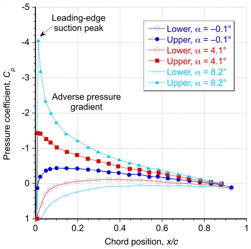
The NACA 0012 is a symmetric airfoil; therefore, at zero angle of attack (or almost at  0.1o in this case), the upper surface pressure distribution is identical to that of the lower surface. Increasing the angle of attack produces significant suction (negative) pressures on the upper surface, the lowest at the leading edge. At an angle of attack of 8.1, the negative pressures reach a peak value of about
  .
.
A representative pressure coefficient distribution around an airfoil in transonic flow is shown in the figure below. Notice in this case that the region of supersonic flow over the leading edge region produces a more uniform low pressure, terminated by an abrupt pressure recovery, a classic signature indicative of the presence of a shock wave. This outcome contrasts with subsonic flow, where the lowest pressure is much closer to the leading edge, resulting in an adverse pressure gradient over most of the chord. The steep adverse pressure gradient near the shock wave makes the boundary layer much more prone to local thickening and often produces flow separation, i.e., the onset of shock-induced separation.
Check Your Understanding #3 – Integrating a pressure distribution
Calculate the lift coefficient and the center of pressure on a two-dimensional body where the pressure coefficient distribution at low angles of attack is described by
![\[ C_{p_{u}} = 1 - A \left( \frac{x}{c} \right)^2 \quad \mbox{for $0 \le x/c \le 0.1$} \]](https://eaglepubs.erau.edu/app/uploads/quicklatex/quicklatex.com-ab41b8472feb1513b662fc90f5b37d95_l3.svg "Rendered by QuickLaTeX.com")
![\[ C_{p_{u}} = B \left( \frac{x}{c} -1 \right) \quad \mbox{for $0.1 < x/c \le 1.0$} \]](https://eaglepubs.erau.edu/app/uploads/quicklatex/quicklatex.com-61d67ce30388dc77291fb16835ecd7c9_l3.svg "Rendered by QuickLaTeX.com")
![\[ C_{p_{l}} = 1 - C \left( \frac{x}{c} \right) \quad \mbox{for $0.0 \le x/c \le 1.0$} \]](https://eaglepubs.erau.edu/app/uploads/quicklatex/quicklatex.com-da7999c4b0d01b17f3cea29068f1c3cd_l3.svg "Rendered by QuickLaTeX.com")
where  = 300,
  = 2.2277 and
  = 0.95.
Show solution/hide solution.
The lift coefficient is given by
![\[ C_l = \int_0^1 \Delta C_p \, d(x/c) = \int_0^1 (C_{p_{l}} - C_{p_{u}}) \, d \overline{x} \]](https://eaglepubs.erau.edu/app/uploads/quicklatex/quicklatex.com-d941d8fcb06572930054990176a9f2ca_l3.svg "Rendered by QuickLaTeX.com")
For this problem, it can be split into two integrals, i.e.,
![\[ C_l = \int_0^{0.1} (C_{p_{l}} - C_{p_{u}}) d \overline{x} + \int_{0.1}^1 (C_{p_{l}} - C_{p_{u}}) d \overline{x} = C_{l_{1}} + C_{l_{2}} \]](https://eaglepubs.erau.edu/app/uploads/quicklatex/quicklatex.com-81663f09a2d9aa0e345c63202769d297_l3.svg "Rendered by QuickLaTeX.com")
Taking the first integral gives
![\[ C_{l_{1}} = \int_0^{0.1} (C_{p_{l}} - C_{p_{u}}) d \overline{x} = \int_0^{0.1} \big( \left( 1 - 0.95 \overline{x} \right) - \left( 1 - 300 \overline{x} ^2 \right) \big) d \overline{x} \]](https://eaglepubs.erau.edu/app/uploads/quicklatex/quicklatex.com-4953d9efe18a6cb4ecfb1c72036005cc_l3.svg "Rendered by QuickLaTeX.com")
and so
![\[ C_{l_{1}} = \int_0^{0.1} \left( 300 \overline{x} ^2 - 0.95 \overline{x} \right) d \overline{x} = \Bigg[ 100 \overline{x}^3 - 0.475 \overline{x}^2 \Bigg]_{0}^{0.1} = 0.09525 \]](https://eaglepubs.erau.edu/app/uploads/quicklatex/quicklatex.com-9ffe9b90333243dfe6117db653a015ab_l3.svg "Rendered by QuickLaTeX.com")
Taking the second integral gives
![\[ { C_{l_{2}} = \int_{0.1}^{1} (C_{p_{l}} - C_{p_{u}}) d \overline{x} = \int_{0.1}^{1} \big( \left( 1 - 0.95 \overline{x} \right) - \left( -2.2277 + 2.2777 \overline{x} \right) \big) d \overline{x} } \]](https://eaglepubs.erau.edu/app/uploads/quicklatex/quicklatex.com-dc712eced4ede324efc0402b46fc71e4_l3.svg "Rendered by QuickLaTeX.com")
and so
![\[ C_{l_{2}} = \int_{0.1}^{1} 3.2277 \left( 1- \overline{x} \right) d \overline{x} = \Bigg[ 3.2277 \left( \overline{x} - \frac{\overline{x}^2}{2} \right) \Bigg]_{0.1}^{1} = 1.307 \]](https://eaglepubs.erau.edu/app/uploads/quicklatex/quicklatex.com-c1584335e3ad4a66095f52538b68d868_l3.svg "Rendered by QuickLaTeX.com")
Therefore, adding the two parts of the integral gives
![\[ C_{l} = C_{l_{1}} + C_{l_{2}} = 0.09525 + 1.307 = 1.4025 \]](https://eaglepubs.erau.edu/app/uploads/quicklatex/quicklatex.com-ca9813b0174cb5fafe40b9b1952cbe02_l3.svg "Rendered by QuickLaTeX.com")
The center of pressure location is obtained from the first moment of the pressure difference about the leading edge, i.e.,
![\[ \frac{x_{cp}}{c} = \frac{\displaystyle{\int_0^1 (C_{p_{l}} - C_{p_{u}})\, \overline{x}\, d\overline{x}}}{C_l} \]](https://eaglepubs.erau.edu/app/uploads/quicklatex/quicklatex.com-8a44143815fc77719d51ea49b60b1408_l3.svg "Rendered by QuickLaTeX.com")
For the first interval, then
![\[ \int_0^{0.1} (C_{p_{l}} - C_{p_{u}})\, \overline{x}\, d\overline{x} = \int_0^{0.1} \left( 300 \overline{x}^3 - 0.95 \overline{x}^2 \right) d\overline{x} = \Bigg[ 75 \overline{x}^4 - \dfrac{0.95}{3}\overline{x}^3 \Bigg]_0^{0.1} = 0.00718 \]](https://eaglepubs.erau.edu/app/uploads/quicklatex/quicklatex.com-1f600c57ebd29e9da83513439055512b_l3.svg "Rendered by QuickLaTeX.com")
For the second interval, then
![\[ \int_{0.1}^{1} (C_{p_{l}} - C_{p_{u}})\, \overline{x}\, d\overline{x} = \int_{0.1}^{1} 3.2277(\overline{x} - \overline{x}^2) d\overline{x} = 3.2277 \Bigg[ \dfrac{1}{2}\overline{x}^2 - \dfrac{1}{3}\overline{x}^3 \Bigg]_{0.1}^{1} = 0.52289 \]](https://eaglepubs.erau.edu/app/uploads/quicklatex/quicklatex.com-2c2914d851c0d9bff77cfa08012d9c47_l3.svg "Rendered by QuickLaTeX.com")
Therefore, the total moment is
![\[ \int_0^1 (C_{p_{l}} - C_{p_{u}})\, \overline{x}\, d\overline{x} = 0.00718 + 0.52289 = 0.53007 \]](https://eaglepubs.erau.edu/app/uploads/quicklatex/quicklatex.com-4544ad14548da52bc538a7893d7794c9_l3.svg "Rendered by QuickLaTeX.com")
and so
![\[ \frac{x_{cp}}{c} = \frac{0.53007}{1.4025} \approx 0.378 \]](https://eaglepubs.erau.edu/app/uploads/quicklatex/quicklatex.com-4c3473b2818494c07641336bd445e259_l3.svg "Rendered by QuickLaTeX.com")
Numerical Integration of Pressure
Rarely are analytic (continuous) pressure distributions available about a body, as in the preceding example. Pressure values are typically known at discrete points, such as those obtained from measurements on a wing in a wind tunnel or from computational fluid dynamics (CFD) calculations. Therefore, if the lift and moment coefficients are to be obtained from the pressure distributions, then a numerical integration approach must be adopted. It is generally impossible to determine the drag this way; however, using measurements, a momentum-deficiency approach is usually employed.
The lift force coefficient, , can be determined by evaluating the integral
(38) 
which will be apparent as just the area under the versus the curve.
The easiest numerical integration method to find an area (which also has good accuracy) is to use the trapezoidal rule, where the integral is written as a numerical summation, i.e.,
(39) 
where is the number of discrete points for which or  is known. The process is shown in the figure below. Notice that
  is an index, i.e.,
  , and that for points, there would be
  incremental area contributions to the integral. The more points available with pressure values, the more accurate the numerical integration will be.
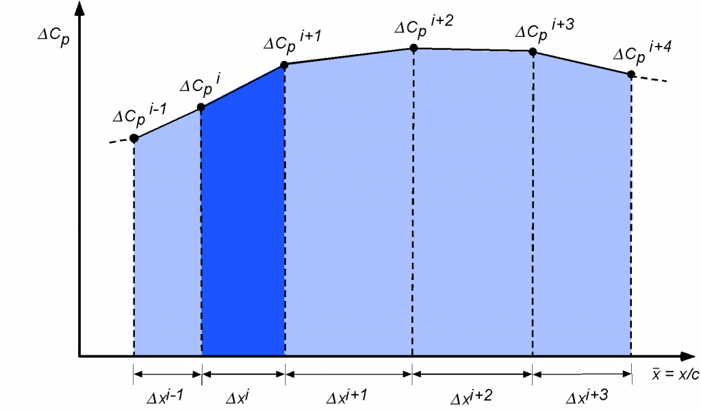
The preceding is a satisfactory approach if the values of  are known along the chord at all discrete points (both on the upper and lower surfaces). The problem is that pressure points are available at different values of on the upper and lower surfaces. This means that the integral (area under the curve) must be found in two parts, i.e., a numerical summation of the like
(40) 
where  is the number of points on the upper surface and
  is the number of points on the lower surface, as shown in the figure below.
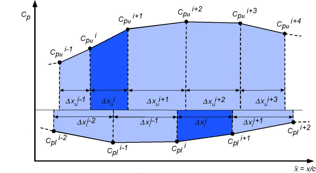
The corresponding pitching moment about the leading edge of the airfoil can be determined from
(41) 
An extra  term appears in the equation, representing the moment arm. Notice the sign on the pitching moment, which can be recalled as being positive in a nose-up sense. Again, this latter integral would be converted to a numerical summation where the moment arms will be included in the summation, which is calculated at the mid-point of each trapezoid, i.e., giving an equation of the form
(42) 
The pitching moment about the 1/4-chord can be determined from
(43) 
After that, the pitching moment about any other point can be found by using simple statics from the values of and , i.e., for the moment about a point that is a non-dimensional distance from the leading edge, then
(44) 
Finally, the axial force (or chord force) coefficient can be determined by evaluating
(45) 
where  . Again, this integral will be evaluated numerically using the trapezoidal rule, but this is not an easy one to integrate because not only is the shape of the airfoil needed (i.e., values and the slope of the surface) but a lot of points is needed around the nose of the airfoil (where there are steep pressure gradients and relatively high values of surface curvature) to get good accuracy, as shown in the figure below. Caution should also be exercised to ensure the correct signs (positive or negative) are used.
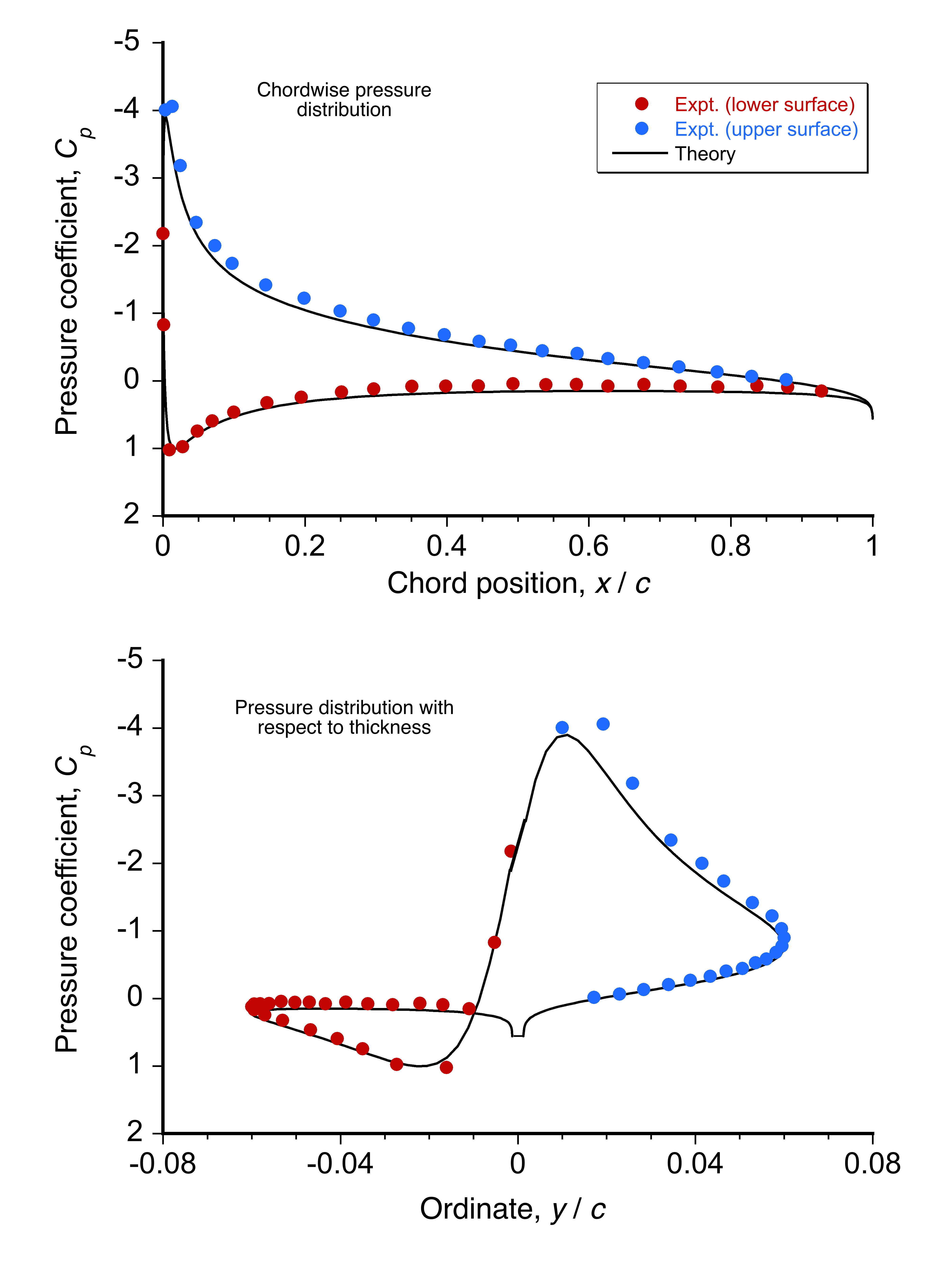
Check Your Understanding #4 – Numerically integrating a pressure distribution
Write some MATLAB code to plot the chordwise form of the pressure distribution in Example #3 and perform the integration numerically to find the lift. Hint: MATLAB has a handy function called “trapz” to do this.
Show solution/hide solution.
Some MATLAB code is provided below; you can copy and paste it into your version of MATLAB. Running the code gives = 1.4025, which agrees with the value from the analytic integration given in Worked Example #3. Of interest is varying the number of points used in the linspace function for numerical integration.
clc
figure
axis([0.0 1.0 1.0 5.0])
x1 = linspace(0,0.1,500);
x2 = linspace(0.1,1,500);
cpu_1 = 1.-300*x1.^2;
cpu_2 = -2.2277 + 2.2777.*x2;
x = [x1 x2];
cpu = [cpu_1 cpu_2];
cpl = (1.0-0.95*x);
dcp = cpl-cpu;
trapz(x,dcp) % to find the section cl using the trapezoidal rule
plot(x,cpu);hold on
plot(x,cpl)
xlabel(‘x/c’)
ylabel(‘C_P’)
legend(‘Upper surface’, ‘Lower surface’)
Supersonic Airfoils
A supersonic airfoil shape is designed to operate at Mach numbers greater than unity. Unlike subsonic airfoils, supersonic airfoils produce strong shock waves. These shock waves create significant pressure changes, which, in turn, affect the airflow and the aerodynamic performance of the airfoil.
The well-rounded, cambered airfoil sections, which are well-suited to subsonic flight speeds, are generally inappropriate for high-speed and supersonic flight. Supersonic airfoils are distinctive in their geometric shapes in that they are thin (i.e., have a lower thickness-to-chord ratio) with sharp leading edges. Supersonic airfoils generally have thinner sections constructed of angled planes called double-wedge airfoils or opposed circular arcs called biconvex airfoils, as shown in the figure below.
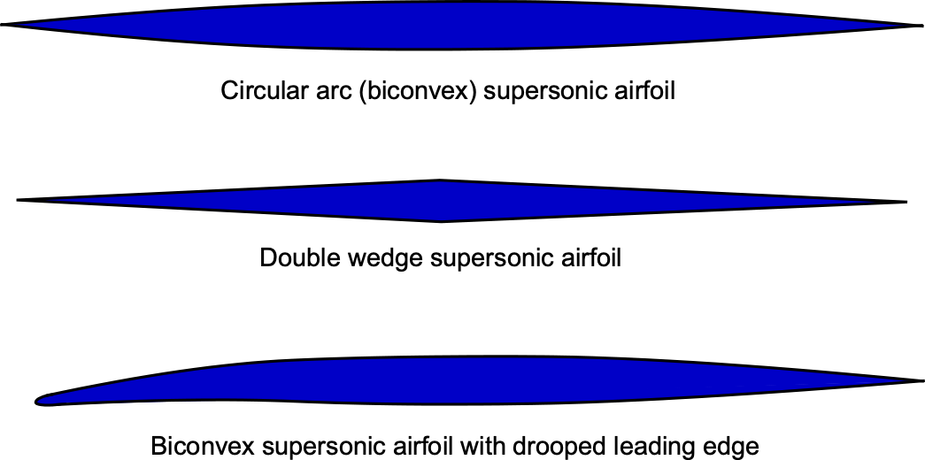
The sharp leading edges on supersonic airfoils prevent the formation of a detached bow shock in front of the airfoil, which is a significant source of drag called wave drag. For example, in the schlieren image below, the supersonic flow passes smoothly over the airfoil’s sharp nose, resulting in minimal drag. For a supersonic airfoil, the thickness and camber shapes are designed to minimize energy losses associated with the compression and expansion of the flow. However, this goal can often be achieved only over a small range of angles of attack.
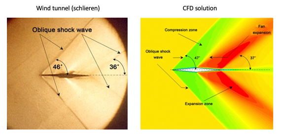
Consider the flow around an airfoil in the form of a double wedge (or diamond) in a supersonic flow, as shown below. Unlike a subsonic airfoil with smooth surface curvature, a double-wedge airfoil is ideal for supersonic flow. Notice that the upstream flow gets no warning of the approaching airfoil in a supersonic flow, so the streamlines have no curvature.
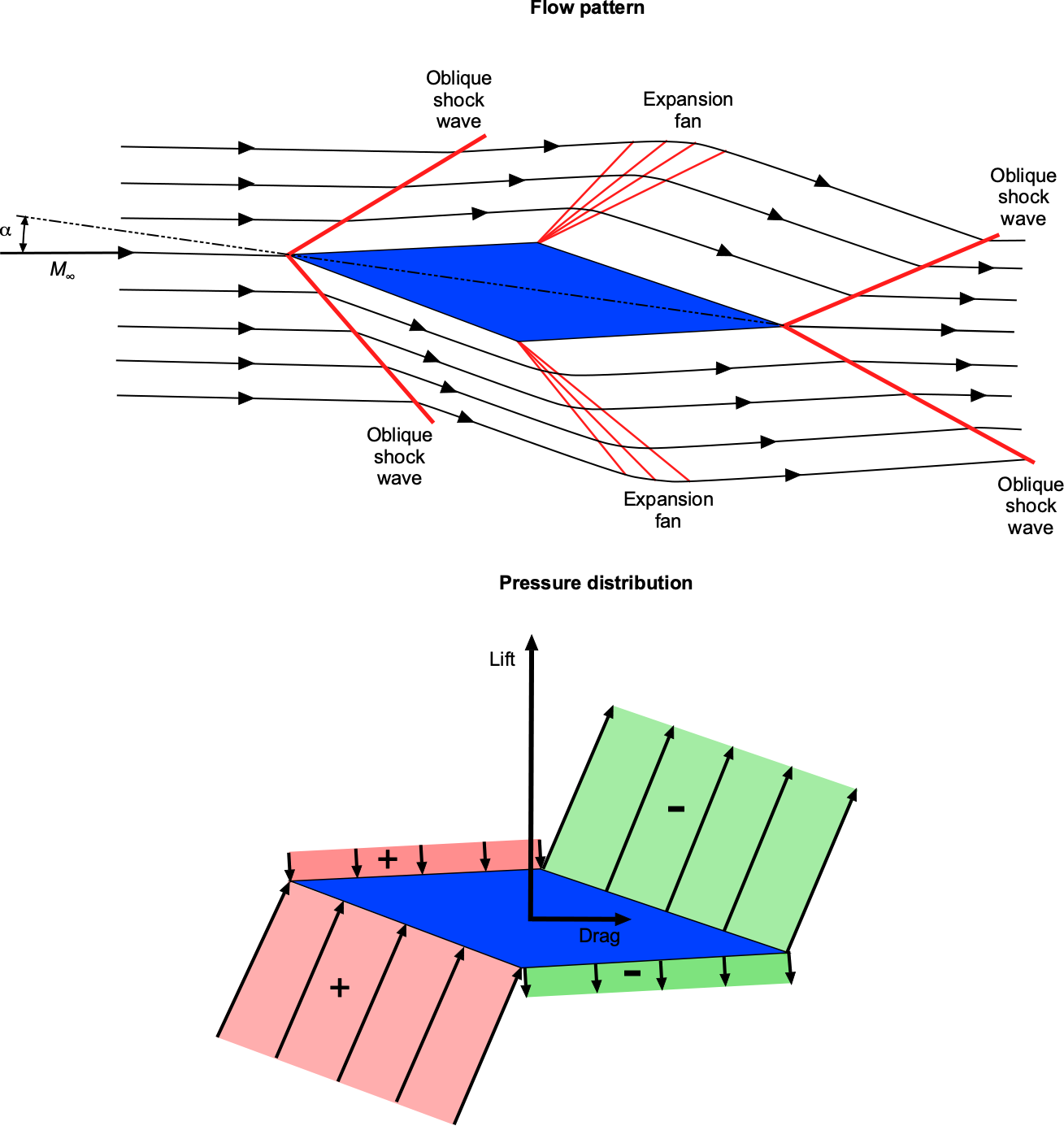
Oblique compression shock waves occur at the leading edge of the airfoil. The Mach number across the shocks decreases (but remains supersonic), and the static pressure increases over the freestream value. Notice the increased pressure on the lower surface, which significantly contributes to the lift. At the points of maximum thickness, expansion waves form, increasing the Mach number and decreasing the pressure after the expansion is complete. The upper surface of the airfoil now contributes to the lift. Rarefaction shock waves form at the trailing edge, increasing the Mach number and returning the pressure to the freestream value.
The linearized supersonic airfoil theory shows that the lift coefficient is independent of the airfoil shape but depends on the angle of attack, , as given by
(46) 
This latter result indicates that the lift-curve slope is lower in supersonic flight than in subsonic flight and decreases with increasing Mach number.
The results in Eq. 15 (subsonic) and Eq. 46 (supersonic) are classical solutions in the airfoil theory and allow the determination of the lift coefficients on airfoils at small angles of attack. These thin-airfoil approximations agree well with measurements of the lift-curve slope made on 2-D airfoils, as shown in the figure below. The linearized supersonic theory also retains good validity when extended to three dimensions, as seen in the prediction of the lift-curve slope of a finite wing with a higher aspect ratio.
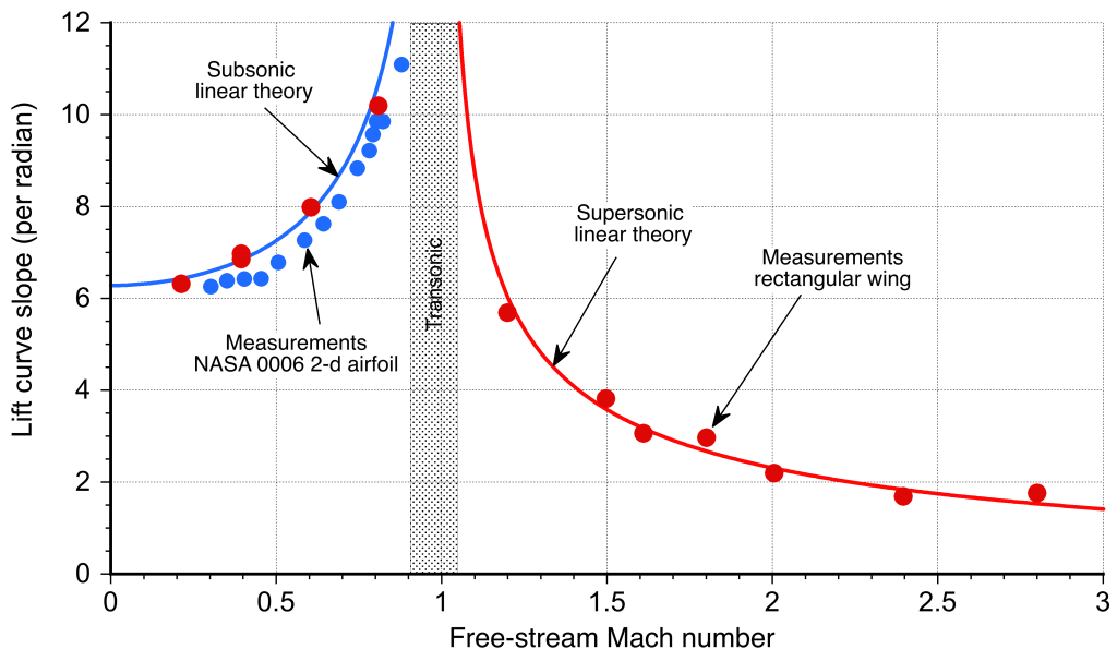
The linearized theory shows that the lift coefficient is independent of the airfoil shape. For example, the lift coefficient produced by a supersonic airfoil at a given angle of attack is the same for a flat plate, a diamond-wedge airfoil, or a biconvex airfoil. The drag, however, is different because the dominant source of drag in supersonic flight is wave drag, which depends strongly on the airfoil shape.
For example, for a diamond-wedge airfoil, the drag coefficient is
(47) 
which shows that wave drag increases with the square of the airfoil’s maximum thickness-to-chord ratio, . In general, the wave drag of a supersonic airfoil can be expressed as
(48) 
where is its maximum thickness-to-chord ratio and  is its maximum camber. The values of the constants
  and
and  depend on the exact shape of the airfoil. Therefore, it becomes clear why the airfoils used on the wings of supersonic airplanes must be very thin and mildly cambered compared to those used on subsonic airplanes.
Check Your Understanding #5 – Calculating the lift & drag coefficients on a supersonic airfoil
A supersonic double-wedge airfoil with a thickness-to-chord ratio of 8% is operated at an angle of attack of 5.0o at a Mach number of 3.5. Calculate the lift-to-drag ratio.
Show solution/hide solution.
In this case, the values given lead to
![\[ \sqrt{M_{\infty}^2 - 1} = \sqrt{3.5^2 - 1} = 3.35 \]](https://eaglepubs.erau.edu/app/uploads/quicklatex/quicklatex.com-4da83a7c439e80fa5fab294e43184fda_l3.svg "Rendered by QuickLaTeX.com")
and
![\[ \alpha = 5.0 \times \frac{\pi}{180} = 0.0873~\mbox{rads} \]](https://eaglepubs.erau.edu/app/uploads/quicklatex/quicklatex.com-21b29021709f4e9a651524a6031f7be4_l3.svg "Rendered by QuickLaTeX.com")
The lift coefficient is
![\[ C_l = \frac{4 \, \alpha }{\sqrt{M_{\infty}^2 - 1}} = \frac{ 4 \times 0.0873}{3.35} = 0.104 \]](https://eaglepubs.erau.edu/app/uploads/quicklatex/quicklatex.com-0edfd0a559516f043e6d57d4a7a36be4_l3.svg "Rendered by QuickLaTeX.com")
The wave drag coefficient is
![\[ C_{d_{w}} = \frac{4}{\sqrt{M_{\infty}^2 - 1}} \bigg( \alpha^2 + \left( \frac{t}{c} \right)^2 \bigg) = \frac{4.0}{3.35} \left( 0.0873^2 + 0.08^2 \right) = 0.0167 \]](https://eaglepubs.erau.edu/app/uploads/quicklatex/quicklatex.com-0b5e05743e70887a0f705dd2b1c06a9b_l3.svg "Rendered by QuickLaTeX.com")
Therefore, the lift-to-drag ratio is
![\[ \frac{C_l}{C_{d_{w}} } = \frac{0.104}{0.0167} = 6.23 \]](https://eaglepubs.erau.edu/app/uploads/quicklatex/quicklatex.com-91c5775dacf77c91689050589f1ccd74_l3.svg "Rendered by QuickLaTeX.com")
A significant problem with thin supersonic airfoils is that at low (subsonic) flight speeds, they tend to produce leading-edge flow separation and stall even at moderate angles of attack. Therefore, many aircraft that employ supersonic airfoils must use high-lift devices for takeoff and landing, such as large leading-edge slats along the entire wing. Another method is to droop the leading edge using camber, which maintains supersonic performance while markedly improving low-speed characteristics. Nevertheless, supersonic aircraft have relatively high takeoff and landing speeds and may require drogue parachutes to reduce landing distance.
Supercritical Airfoils
Because commercial jet airliners need to reach increasingly higher cruise speeds approaching the speed of sound, i.e., for flight at transonic Mach numbers, this requirement has led to the design of unique wing shapes called supercritical wings. A supercritical wing also uses a supercritical airfoil shape to reduce the strength of shock waves, thereby reducing wave drag and increasing the drag divergence Mach number. The principle of this airfoil is illustrated in the figure below, where the upper surface is relatively flat at the leading edge compared to a conventional airfoil.
The classic approach to increasing the drag divergence Mach number is reducing wing thickness, i.e., the maximum thickness-to-chord ratio. However, this has several other disadvantages, including a reduced fuel tank capacity and increased structural weight for the same strength and stiffness. Supercritical airfoils were initially studied in the 1950s by Herbert Pearcey at NPL in England and refined during the 1960s by Richard Whitcomb at NACA. Today, supercritical airfoils are used on nearly all commercial jet aircraft, enabling them to cruise at higher flight Mach numbers, typically between 0.8 and 0.85.
A supercritical airfoil shape is notably distinctive. It has a point of maximum thickness fairly aft on the chord, with a relatively flat upper surface with a slight camber. The aerodynamic principle used in transonic wing and airfoil design is to control the flow’s expansion to supersonic speed and its subsequent recompression, thereby making the leading-edge pressure distribution less “peaky” and more uniform. The small amount of leading-edge camber helps limit the strength of the shock waves at the expense of some loss of lift at a given angle of attack. However, such transonic airfoils have significant camber at their trailing edges, which helps recover the lost lift.
The net effect is a significant increase in the critical Mach number and drag divergence Mach number, as shown in the figure below. Increasing the critical Mach number allows the aircraft to operate at higher speeds without encountering excessive drag or other aerodynamic issues associated with transonic flight. However, the drag divergence Mach number can vary with various design factors, including the thickness-to-chord ratio, . A supercritical airfoil generally limits the onset of drag divergence to a higher freestream Mach number. It improves the aerodynamic performance of aircraft that operate near the speed of sound.
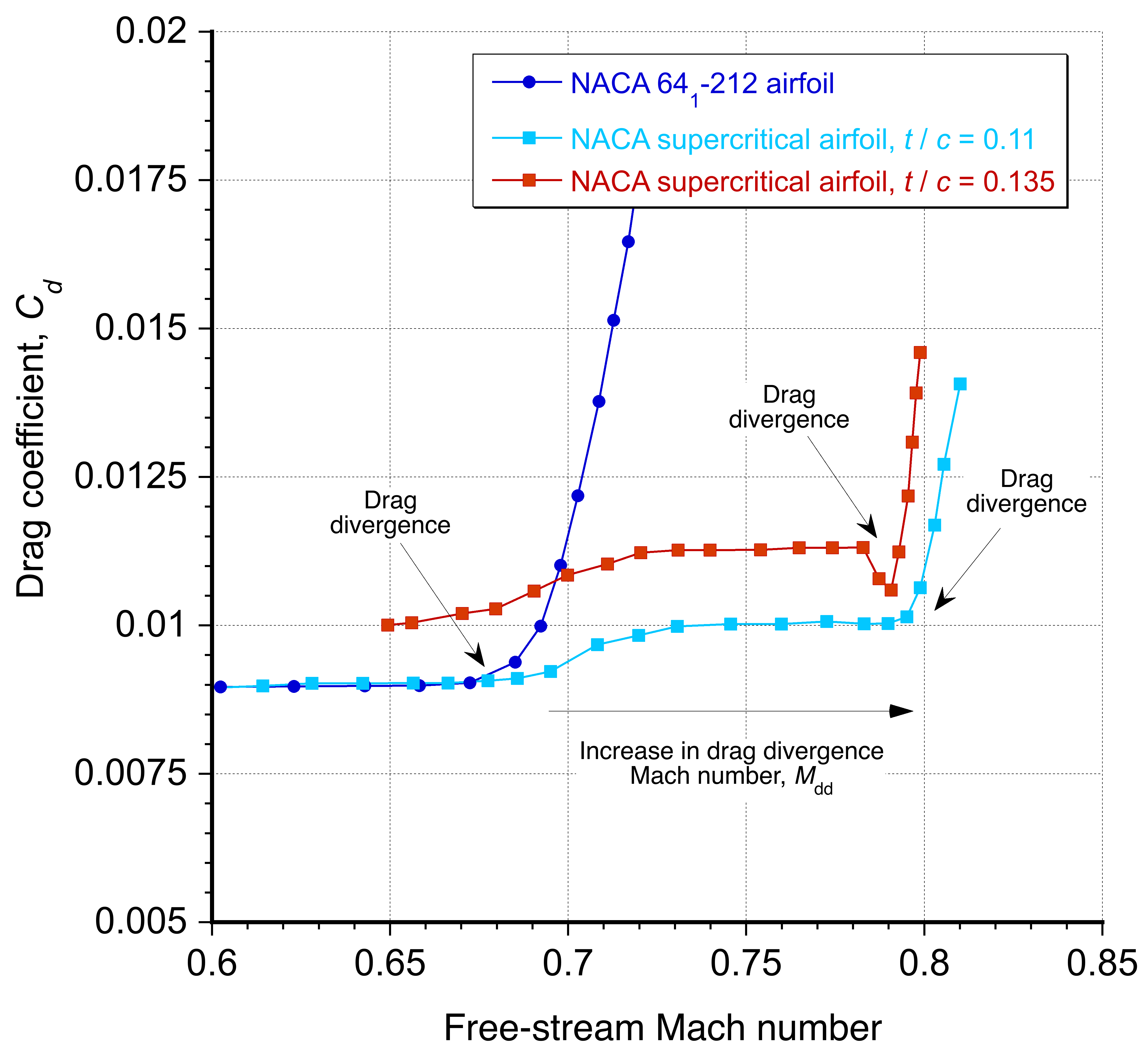
Observing a Shockwave on an Airliner’s Wing
When cruising in an airliner at Mach 0.8 and looking out of the window, a faint shadow or shimmering band on the wing may be visible, as shown in the figure below. What is seen here is the optical effect of the upper-surface shock wave. For a transonic supercritical wing, this shockwave is located quite far back from the leading edge, often near the mid-chord. The physics behind this observed effect can be explained by the changes in air density and the refraction of light rays as they travel through regions of varying flow density.
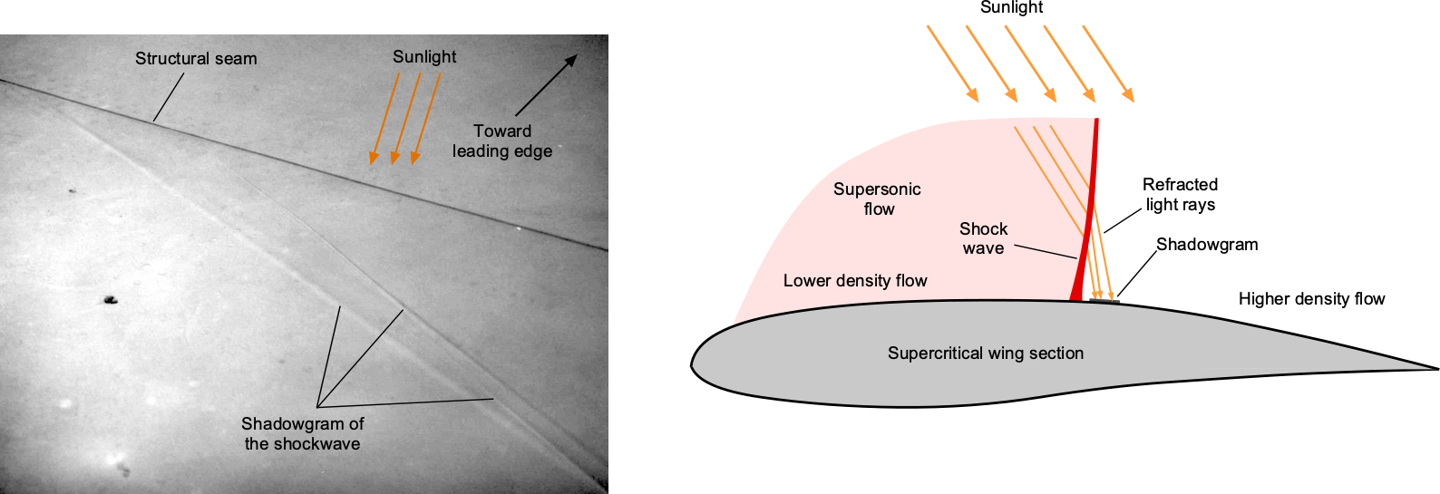
At cruise, the flow over the upper surface of the wing accelerates to supersonic speeds and then returns to subsonic speed as it passes through a shock wave. Across this thin shock, the air density increases abruptly, say from  to
to  . Because the refractive index of air depends on its density according to the Gladstone-Dale relation, i.e.,
(49) 
then there is an associated jump in the refractive index of the air, i.e.,
(50) 
Whenever light passes through a region where the refractive index changes according to Snell’s law, i.e.,
(51) 
where  and
and  are the refractive indices on either side of the shock wave, and
  and
and  are the angles of the ray before and after refraction. For small angles, the deflection angle can be approximated by
(52) 
Sunlight streaming past the airplane is, therefore, bent by small angles where it crosses the shock wave, and it also incurs a small change in optical path. Along each ray, the optical path length is
(53) 
where  is the local refractive index and
  is an element of distance along the ray, so the shock wave introduces an optical-path difference given by
(54) 
where  is the effective thickness of the shock wave along the line of sight. The transverse gradient of refractive index bends the rays so that, before reaching the wing surface and the observer’s eye, neighboring rays diverge or converge slightly. The recorded brightness variation
  scales with the second derivative of the refractive index, i.e.,
(55) 
where  is the transverse coordinate normal to the shock and
  is the line-of-sight coordinate. This quantity is relatively large even in the presence of a weak shock. Where the bundle of rays diverges, the surface appears darker, and where it converges, it appears brighter. The result is a visible spanwise stripe across the wing that shifts as the shock position changes with changes in airspeed or wing angle of attack.
This shadow should not be mistaken for a surface feature of the wing, such as a structural seam or joint, but the direct manifestation of the refraction of light across the shock wave. It constitutes a natural shadowgraph, in which the Sun serves as the light source, the shock acts as the optical interface that bends the rays, and the human eye functions as the detector along the optical path. In this way, the physics of a compressible flow can be observed directly, using nothing more than sunlight and access to a passenger window.
Inverse Airfoil Design and Shape Optimization
Inverse airfoil design aims to determine the shape of an airfoil that achieves the desired level of aerodynamic performance. By using inverse design,[2] airfoil shapes can be tailored to achieve specific aerodynamic goals, such as minimizing drag, maximizing lift, minimizing pitching moments, maximizing lift-to-drag ratios, achieving a desired pressure distribution, or maximizing the critical Mach number. This optimization process of the lifting surface(s) may have multiple aerodynamic design goals and can lead to more efficient aircraft or other aerodynamic components.
General Approach
The aerodynamic shape optimization process requires defining an objective function, parameterizing the airfoil’s shape mathematically, applying formal optimization algorithms, and then iterating (carefully!) until an optimal airfoil design shape is achieved. The process combines aerodynamic solutions, optimization techniques, and sensitivity analysis to refine the airfoil shape, ensuring it meets the specified performance goals. Airfoil shape optimization is often conducted at a given angle of attack or lift coefficient. Airfoil sections are very much “point designs,” but shape optimization must also account for off-design aerodynamic performance. In this regard, off-design operation is often referred to as “robustness.” Some level of robustness is desired because an aircraft can never operate precisely at the design point.
The shape optimization process involves:
- Establish the desired aerodynamic characteristics, such as the pressure distribution
 , lift coefficient, and/or drag coefficient, and/or pitching moment.
 - Specify the boundary and flow conditions, including freestream velocity, angle of attack, Mach number, and Reynolds number. These parameters have a significant impact on aerodynamic performance and must be considered in the design process.
- Use a panel method to solve for aerodynamics, in which the airfoil shape is discretized into panels, and integral equations are solved to find the resulting pressure distribution. Alternatively, consider using computational fluid dynamics (CFD), although this approach will be significantly more time-consuming.
- Implement optimization algorithms to adjust the airfoil shape based on performance goals. This typically involves iterative algorithms that adjust shape parameters based on performance criteria.
- Adjust the airfoil shape to minimize the difference between the desired and actual performance.
- Validate the design using wind tunnel testing to ensure the airfoil meets the desired performance levels.
Shape optimization involves finding the airfoil shape that meets the performance goals. In this regard, an objective function  is used to quantify the difference between the desired and actual performance. For a pressure distribution, say
  , this can be expressed as
(56) 
where  is the desired or “design” pressure distribution, and
  is the actual or current pressure distribution for the given shape. Any constraints that the shape must satisfy, such as geometric and aerodynamic constraints, can now be introduced. For example, constraints may be placed on the maximum or minimum thickness-to-chord ratio, e.g., for structural reasons, the amount of camber, or both. The feasibility of manufacturing the shape may also be considered a design constraint, especially when different airfoils are used along the span of a wing or other lifting surface, such as a propeller, helicopter rotor, or wind turbine blade.
Typically, the airfoil’s shape must be parameterized mathematically using a set of shape variables. If control points or coefficients describe the shape, it can be expressed in the form
(57) 
where  is the modified shape of the airfoil,
  is the initial or baseline shape of the airfoil,
  are shape parameters that control the contribution of each basis function, and
  are basis functions that describe how the shape is modified. For example, in the case of using a standard Fourier series
(58) 
where  represents the location of the upper and lower surfaces of the airfoil,
  ,
,  , and
, and  are coefficients of the Fourier modes of frequency that can be used to adjust the shape of the airfoil, and
  and
and  are referred to as the basis functions used to represent the shape.
Well-established gradient-based optimization methods can then be used to compute the gradient of the objective function with respect to the shape parameters that describe the airfoil. The shape parameters can then be updated using
(59) 
where  is a coefficient, often called a relaxation parameter, which is used to define the new shape of the airfoil to meet the specific aerodynamic requirements. Typically, the relaxation parameter should be kept relatively small, e.g., less than 0.05, to prevent significant shape changes to the airfoil during any design iteration, which could cause the method to fail. As part of the process, changes in shape parameters can be explored to see how they affect the objective function, with sensitivity determined by
  .
.
Finally, the shape parameters are updated using the optimization algorithm, allowing the objective function to be recalculated. This process can be continued until the convergence criteria are met, i.e.,  , where
  is an acceptable tolerance level based on the design goals. If the process runs smoothly, the numerical approach and shape changes must be carefully monitored to obtain the new airfoil shape.
The figure below shows representative outcomes of this process for a transonic airfoil section. The initial “conventional” airfoil shape exhibits a strong shock wave and a relatively low drag-divergence Mach number. The optimization goal is to maximize the drag divergence Mach number while maintaining a thickness-to-chord ratio of at least 13% for structural purposes. The optimization process results in an airfoil with a flatter upper surface. This design modification results in a weaker shock wave and a higher drag divergence Mach number, thereby enhancing the airfoil’s performance at transonic speeds. Additionally, the trailing edge of the optimized airfoil exhibits increased camber, improving aerodynamic efficiency while satisfying the structural constraint.
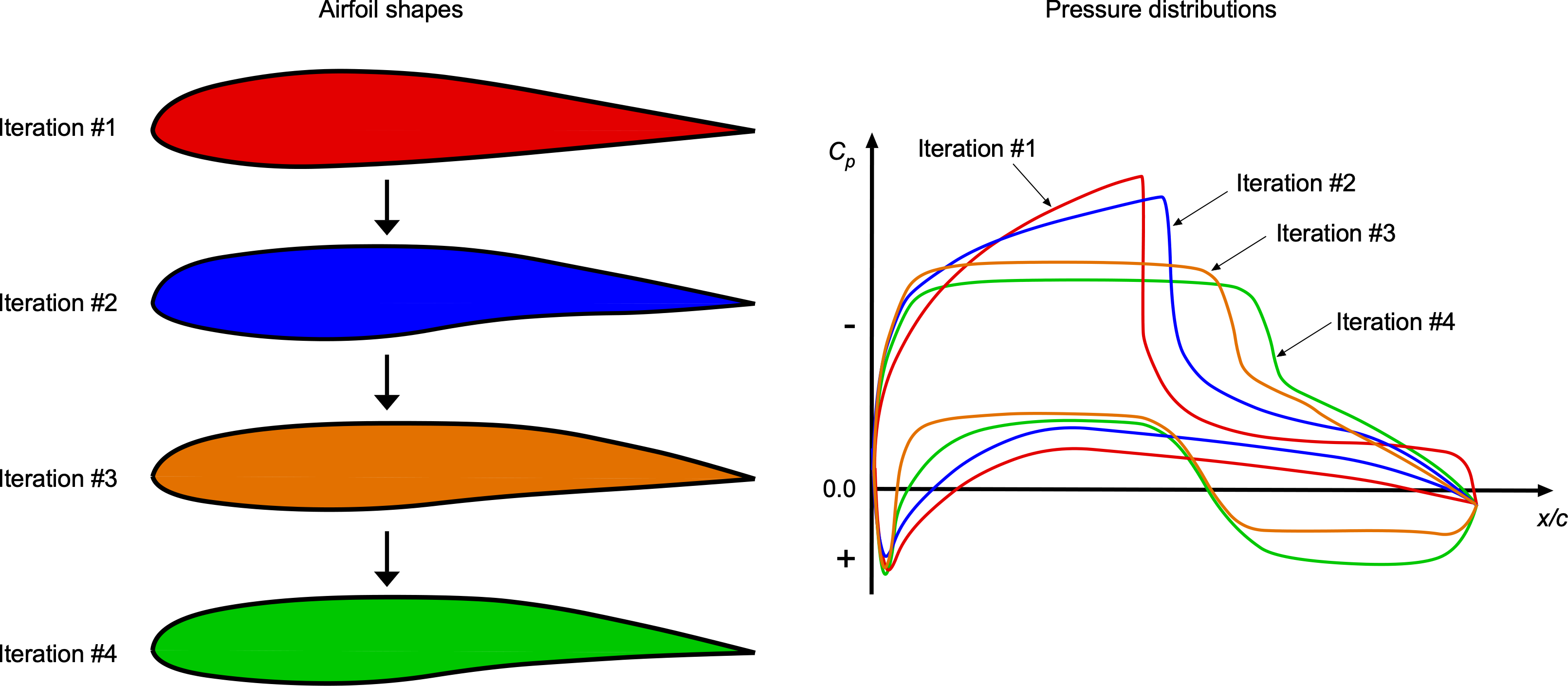
Successful outcomes for the optimized airfoil shape depend on the fidelity of the optimization process, the accuracy of the aerodynamic simulations, and the practical feasibility of the optimized airfoil design. Wind tunnel testing, if available, can verify the aerodynamic performance by placing a scaled or full-sized wing section model in a controlled airflow environment. Pressure measurements over the surface of the airfoil can be compared with the predictions made, and any aerodynamic improvements can be quantified against the original baseline airfoil. While the method for optimizing the airfoil shape is well-established and relatively quick, the wind-tunnel verification process may be much longer.
Rooftop & Stratford Pressure Distributions
The upper surface or suction-side pressure distribution governs the state of the boundary layer and, therefore, the attainable lift of an airfoil. A design principle useful for both laminar and turbulent boundary layers is to allow the boundary layer to develop such that it is always just below the conditions for the onset of flow separation. In this way, the suction pressure can be maximized over a larger portion of the surface, thereby generating the maximum possible lift from the airfoil.
Two canonical design conditions are of interest. The first condition is the laminar “rooftop” constant-pressure condition, which maintains the laminar boundary layer for as long as possible to minimize skin friction. The second condition is the Stratford turbulent recovery, which prescribes the steepest adverse pressure gradient that a turbulent boundary layer can withstand without separating. Inverse design methods for airfoil shapes typically allow combining the two conditions in sequence. Hence, the suction side maintains nearly constant suction pressure upstream of the transition point and then recovers according to Stratford’s recovery criterion downstream.
Stratford’s turbulent separation criterion[3] was derived using the boundary layer equations in conjunction with turbulent boundary layer measurements in adverse pressure gradients, and it remains one of the most useful results in practical aerodynamics. Starting from the suction peak at  , where the velocity has reached its maximum and the pressure its minimum, the criterion states that subsequent recovery must satisfy
(60) 
where  is an empirical constant, for which
  is used for most applications. Equation 60 expresses the combination of pressure and pressure gradient that will lead to the onset of flow separation. Once and the overall recovery endpoint are specified, the criterion states that there exists only one pressure distribution that keeps the turbulent boundary layer attached. If the pressure recovery is more adverse, the flow separation will occur, resulting in a loss of lift and an increase in drag.
A reparameterization of the Stratford criterion is useful for inverse airfoil design methods, which is obtained by defining
(61) 
where  is the local flow velocity at the edge of the boundary layer, together with an effective length
  measured from the leading edge suction peak. The Stratford criterion then takes the form
(62) 
where  is a Reynolds number based on the peak velocity, and
  is an empirical constant of order unity that depends on the surface curvature. Another formulation, attributed to Cebeci and Smith,[4] incorporates the effective development length of the turbulent boundary layer, which accounts for the accumulated history of the adverse environment, i.e.,
(63) 
This refined criterion is relevant when the transition occurs just upstream of the recovery because it adjusts the separation limit to reflect the relatively short development of the turbulent layer. In practice, Stratford’s criterion has been found to be conservative, i.e., predicting separation slightly earlier than it occurs. By shaping the suction-side pressure recovery to follow this criterion, inverse design methods[5] produce airfoil shapes that can generate high lift coefficients before flow separation occurs.
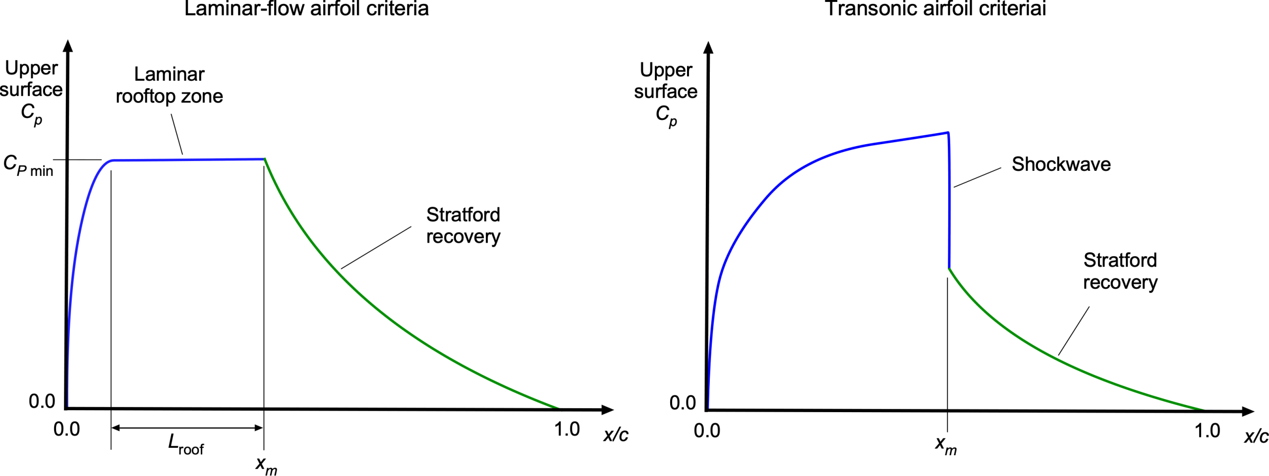
A laminar boundary layer cannot withstand a strong pressure recovery. Therefore, to encourage the development of a laminar boundary layer, the suction side is shaped into a constant pressure of “rooftop” distribution, as shown in the figure below. After the leading-edge acceleration has produced a suction peak at , the external velocity is held nearly constant downstream, i.e.,  and
and  constant so that the laminar boundary layer is just on the verge of separation. Any attempt to recover too early causes laminar separation, so the flat plateau is the ideal form.
The extent of the rooftop region, defined by  , and its length
  are the key design variables. At typical Reynolds numbers, the suction peak occurs at
  0.07–0.15, with a stable rooftop region extending to 0.15–0.60 to the transition point. Lower suction pressures result in higher lift coefficients but induce earlier transition and may also increase the airfoil’s sensitivity to surface roughness. Shallower rooftops extend the laminar flow and reduce drag, but limit the attainable maximum lift coefficient. The design of a laminar-flow airfoil is therefore a composite exercise: the suction side is given a rooftop plateau extending from to a thw transition point
  , beyond which the recovery follows Stratford’s law, prescribing the steepest pressure rise a turbulent boundary layer can withstand before separating.
Compressibility effects impose further limits on airfoil design. At transonic Mach numbers ( 0.75–0.85), a deep rooftop produces a supersonic pocket that terminates in a shock, and shock-boundary-layer interaction often triggers flow separation before Stratford’s criterion is even reached. The suction-side sequence then consists of rapid acceleration to the rooftop pocket, a terminating shock, and a turbulent recovery downstream. Upstream, the rooftop must be moderated to keep the shock weak and attached, while downstream, the Stratford recovery must be relaxed to account for compressibility and the thickened boundary layer. The ultimate limit on lift in this regime is therefore set by both the onset of turbulent separation and shock-induced flow effects.
Summary & Closure
Understanding the aerodynamic characteristics of two-dimensional (2-D) airfoil sections is a prerequisite for understanding those of finite wings. While airfoil characteristics can be predicted, the most reliable results still come from wind-tunnel measurements, especially near the maximum lift coefficient or during stall. Naturally, the importance of testing techniques in this context must be acknowledged, and airfoil measurements must be made carefully using established methods. Nevertheless, most of the understanding of airfoil section characteristics, including the effects of geometric shape, has come from measurements.
Engineers need to know how to interpret and use 2-D airfoil characteristics. To this end, the ability to access, analyze, and use graphs from catalogs of airfoil characteristics is critical. For example, in a design problem, it may be necessary to select an airfoil shape to meet a set of aerodynamic requirements. Quantities such as the maximum lift coefficient, minimum drag coefficient, and maximum lift-to-drag ratio are necessary for quantifying the aerodynamic characteristics of airfoils. They can also serve as a basis for airfoil selection. In some cases, the characteristics of candidate airfoils may need to be compared, which should always be done on a non-dimensional basis using force and moment coefficients, as well as in the form of drag polars.
5-Question Self-Assessment Quickquiz
For Further Thought or Discussion
- Research how lift and drag measurements of a “two-dimensional” airfoil section could be best performed in a wind tunnel environment.
- Explain why the aerodynamic center for an airfoil moves aft on the airfoil with increasing freestream Mach number. Hint: Consider the nature of the pressure distributions in subsonic, transonic, and supersonic flow.
- What is the role of the angle of attack in determining the characteristics of an airfoil section?
- Can you explain the terms “stall” and “critical angle of attack” in the context of airfoil sections?
- How do airfoil sections contribute to the efficiency and performance of aircraft wings?
- What factors affect the lift-to-drag ratio of an airfoil section?
- Describe the phenomenon of boundary layer separation and explain its impact on airfoil performance.
- Research shadowgraph and schlieren flow visualization systems for use in the wind tunnel. What are their relative advantages, and which one may be preferred?
- The integration of pressure to find lift is usually numerically accurate and successful, but what is the most reliable method for finding drag?
Other Useful Online Resources
Check out some of these additional online resources about the aerodynamics of airfoil sections:
- Smoke flow visualization video of wing stall.
- Aerodynamics – pressure profile around airfoil – a video by the NACA.
- Video: Wind tunnel pressure data for a NACA 0012 symmetric airfoil
- Video on understanding aerodynamic lift.
- With this simulation, you can investigate how a wing produces lift and drag.
- Prandtl-Glauert rule video from GaTech.
- Video: Wind tunnel pressure data for a NACA 0012 symmetric airfoil.
- Where
 means conditions at "infinity" or just far away from the wing where there is an undisturbed "freestream" flow. ↵
 - See: "Robust Aerodynamic Shape Optimization—From a Circle to an Airfoil," X. He, J. Li, C. A. Mader, A. Yildirim, and J. R. R. A. Martins, Aerospace Science and Technology, 8748–61, 2019, doi:10.1016/j.ast.2019.01.051 ↵
- Stratford, B. S., "The Prediction of Separation of the Turbulent Boundary Layer," Journal of Fluid Mechanics, Vol. 5, 1959, pp. 1–16. ↵
- Cebeci, T., & Smith, A. M. O., Analysis of Turbulent Boundary Layers, Academic Press, New York, NY, 974, pp. 341–349. ↵
- See: Eppler, R., Airfoil Design and Data. Springer-Verlag, Berlin, 1990. (Provides comprehensive use of rooftop distributions and Stratford recoveries in inverse airfoil design). ↵
