30 Viscous-Dominated Flows
Introduction
Viscous-dominated flows, often referred to as “creeping” or “Stokes” flows, occur when viscous forces rather than inertial forces predominantly govern fluid motion. These flows are characterized by smooth (laminar), steady, and highly predictable fluid motion. This flow regime is quantified by Reynolds numbers ( ) based on a length dimension,
  , of much less than one (
 ), where the effects of inertia in the flow are negligible compared to viscous forces. Such conditions often arise in scenarios involving very slow flow velocities, small characteristic length scales, or highly viscous fluids.
At very low values of the Reynolds numbers, the inertial term in the Navier-Stokes equation for fluid motion becomes negligible, and the equations simplify to what is known as the Stokes equation, i.e.,
(1) 
where  is the pressure,
  is the velocity vector, and the term
  represents the viscous terms from the velocity gradients. The Stokes equation defines a balance between the flow’s pressure forces and viscous forces. The absence of nonlinear inertial terms in the Navier-Stokes equation implies that the flow is steady and linear, with any external forces being immediately transmitted through the entire fluid without inducing transient or time-history effects.
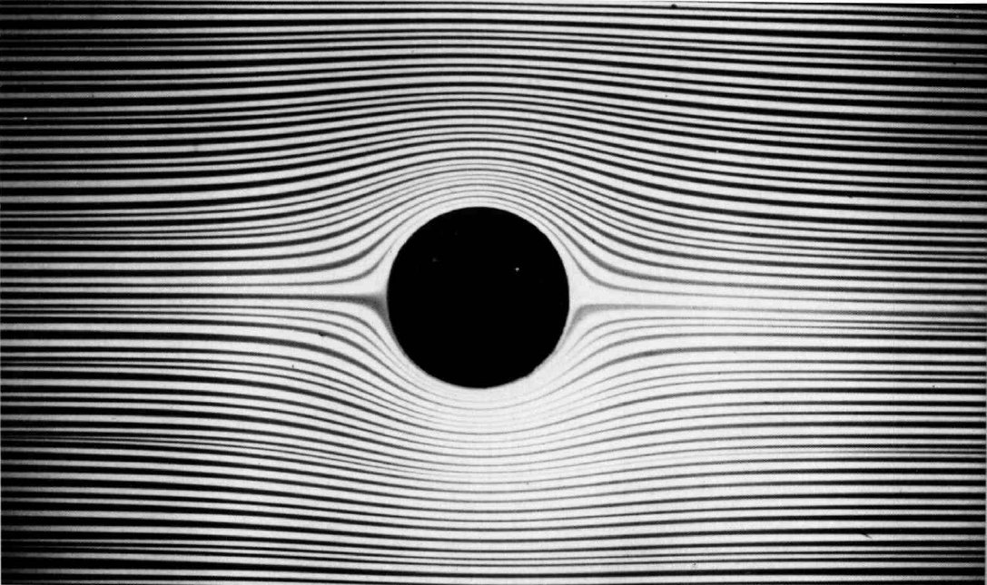
Mathematical models in this flow regime can be used to find closed-form solutions in some cases and allow for easier[1] numerical simulations. One of the defining features of creeping flows is their reversibility. In the absence of inertial effects, reversing the driving force or boundary motion results in the fluid flow that initially developed and then retraces its path exactly. This particular flow behavior contrasts distinctly with higher Reynolds-number flows, where turbulence introduces irreversible flow dynamics. Observations and measurements of creeping flows are abundant in the published scientific literature. [2] highlighting the importance of this type of flow within the framework of the field of fluid mechanics. An example of precise flow visualization of the Stokes flow around the cross-section of a circular cylinder, situated between two glass plates (known as a Hele-Shaw flow), is shown below.
In engineering, creeping flows play a critical role in the study of lubrication, particularly in machinery. Bearings and hydraulic systems rely on these flows to ensure smooth and reliable operation. Highly viscous or creeping flows are also prevalent in natural, biological, and engineering systems. The principles of Stokes flow are also essential in analyzing particle behavior in colloidal suspensions, with applications in pharmaceuticals, food processing, and other industries. Microfluidics represents a modern application of creeping flow, where small fluid volumes are manipulated for various purposes, including the fabrication of microchips for control devices. In aerospace applications, microfluidic systems are increasingly used for thermal management of sensitive electronics, where the dominance of viscous forces ensures precise, stable fluid motion. Applications in biomedical engineering rely on understanding highly viscous flows to analyze blood flow in capillaries and mucus transport in the respiratory system. Similar principles governing creeping flow also apply to various geophysical phenomena, such as the slow movement of glaciers and lava flows.
Learning Objectives
- Develop an understanding of highly viscous creeping flows and the physical conditions under which they occur.
- Reduce the full Navier-Stokes equations to the Stokes equation appropriate for viscous-dominated flow regimes.
- Derive and analyze analytical solutions to the Stokes equations for simple viscous-dominated flow problems.
- Study a class of creeping flow problems called Couette-Poiseuille flows.
- Examine selected aspects of creeping flows in both Newtonian and non-Newtonian fluids.
- Gain an understanding of the fundamental principles of microfluidics and their applications.
Reynolds Number
Recall that the Reynolds number assesses the relative significance of inertial to viscous forces in a fluid. The Reynolds number is expressed as
(2) 
where  is the fluid density,
  is a characteristic velocity, is a characteristic length scale, and
  is the fluid’s viscosity. On the numerator, the grouping
  has units of force (pressure times an area), so in this case, it represents an inertial force, i.e., after the flow is moving, it has the propensity to keep moving. The coefficient of viscosity, , is the shear force per unit area per unit velocity gradient, so the ratio
  has dimensions of a velocity gradient, which is expected based on Newton’s law of viscosity. Therefore, the grouping in the denominator represents a viscous force that acts to retard its motion.
The Reynolds number, therefore, represents a relative measure of inertial to viscous effects in a flow. This dimensionless parameter is widely used in fluid mechanics to classify and analyze flow behavior and predict the transition between laminar and turbulent regimes. In particular, inertial forces are more dominant for  , viscous forces are more dominant, and the flow is steady and laminar.
Low Reynolds Number Flow Around a Sphere
It is instructive to introduce the characteristics of viscous-dominated Stokes flows or creeping flows by considering the Reynolds number-dependent flow around a sphere. The creeping flow around a sphere can also be analyzed using pure mathematics, providing a basis for a general understanding of creeping flows. For a sphere, the characteristic length scale is taken as the sphere’s diameter  , which is a key parameter in determining the flow regime around the body.
At very low Reynolds numbers (), which is usually referred to as the Stokes flow regime, the flow is dominated by viscous forces, where the flow field around the sphere becomes smooth (laminar) and steady, as shown in the figure below. Both spheres and circular cylinders in the low-Reynolds-number regime ( 5) exhibit a unique flow regime in which inertial effects are weak and viscous forces dominate, leading to laminar, predictable flow patterns. In this regime, the flow is characterized by symmetric streamlines around the sphere, with no wake formation or flow separation. At low Reynolds numbers, even as high as = 5, the flow retains Stokes-like characteristics, remaining laminar, with viscous forces shaping the flow patterns, and the streamlines exhibit smooth, symmetric curvature around the sphere. In this range, viscous effects dominate the drag on the sphere, which can be calculated theoretically, leading to Stokes’ drag law.
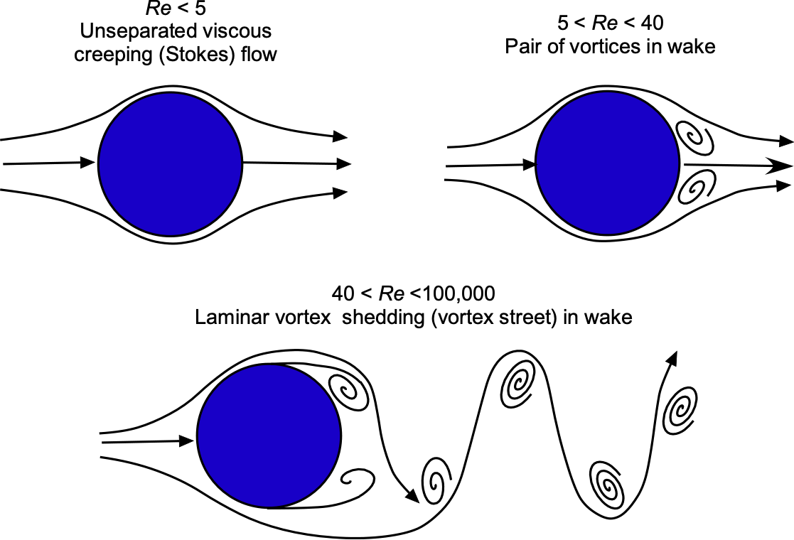
As the Reynolds number increases, the balance of forces shifts, and inertial effects begin to influence the flow. For spheres and circular cylinders, the onset of flow separation occurs at moderate Reynolds numbers ( 5), where a small, symmetric recirculating wake forms behind the sphere, breaking the fore-and-aft flow symmetry observed in the Stokes regime. This new flow becomes increasingly unstable with the onset of periodic vortex shedding at even modestly higher Reynolds numbers. It eventually transitions to a more turbulent flow beyond a critical Reynolds number, typically around
  40, depending on the specific conditions. The distinction between spheres and cylinders lies in their three-dimensional versus two-dimensional geometry, which subtly alters the drag forces and flow patterns but follows the same fundamental principles dictated by the magnitude of the Reynolds number.
Who was George Stokes?
George Gabriel Stokes (1819–1903) was a renowned mathematician and physicist who made significant contributions to fluid dynamics and other fields of science. In 1851, he derived a fluid law, now known as Stokes’ Law, which describes the drag force experienced by a spherical particle moving through a viscous fluid at low Reynolds numbers. Stokes’ contributions laid the groundwork for understanding lubrication, sedimentation, microfluidics, and bioengineering. Stokes held the Lucasian Professorship of Mathematics at the University of Cambridge, where he made significant contributions to fluid mechanics.
Stokes Equation
The Stokes equation is derived by reducing the Navier-Stokes (N-S) equation to exclude the inertia and time-dependent terms. The N-S equation for incompressible flow is given in vector form as
(3) 
where is the fluid density,  is the velocity vector of the fluid, is the pressure field, is the viscosity of the fluid, and
  accounts for external body forces such as gravity. The term
  represents the unsteady or time-dependent change in velocity. In contrast,
  is the nonlinear convective term describing the effects of fluid inertia. The term
  corresponds to pressure-driven forces,
  represents the viscous forces, and introduces any additional external forces acting per unit volume. In addition, for incompressible flows, the density of the fluid remains constant, leading to the incompressible form of the continuity equation, i.e.,
(4) 
This form of the N-S and continuity equations forms the pair of governing equations to describe the motion of incompressible, viscous fluids.
Steady Flow
In the Stokes flow regime, the N-S equation can be simplified. Assume first that the flow is steady. This condition mathematically translates to  , eliminating the unsteady terms from the N-S equation. The second assumption neglects inertial terms, which is valid in the low-Reynolds-number regime. At such small Reynolds numbers, the inertial terms
  become insignificant compared to viscous forces, effectively reducing this term to zero. Under these two assumptions, the N-S equation simplifies significantly to
(5) 
where represents the pressure gradient, accounts for viscous forces, and denotes body forces such as gravity. This equation is usually referred to as Stokes’ equation. If body forces are negligible ( ), the equation further simplifies to
(6)
where the component scalar equations are
(7) ![\begin{align*} \frac{\partial p}{\partial x} &= \mu \left( \frac{\partial^2 u}{\partial x^2} + \frac{\partial^2 u}{\partial y^2} + \frac{\partial^2 u}{\partial z^2} \right) \\[6pt] \frac{\partial p}{\partial y} &= \mu \left( \frac{\partial^2 v}{\partial x^2} + \frac{\partial^2 v}{\partial y^2} + \frac{\partial^2 v}{\partial z^2} \right) \\[6pt] \frac{\partial p}{\partial z} &= \mu \left( \frac{\partial^2 w}{\partial x^2} + \frac{\partial^2 w}{\partial y^2} + \frac{\partial^2 w}{\partial z^2} \right) \end{align*}](https://eaglepubs.erau.edu/app/uploads/quicklatex/quicklatex.com-06e7f95067189a073aea70e6ba5242e4_l3.svg "Rendered by QuickLaTeX.com")
This reduced form of the governing equations highlights a direct balance between pressure gradients and viscous forces, which is the essence of viscous-dominated or creeping flows. The absence of inertial terms ensures that the flow is entirely dominated by viscosity, resulting in a laminar, predictable motion. The incompressible form of the continuity equation, given by  , remains valid for Stokes flow as it does for all incompressible flows.
Unsteady Flow
If the flow is unsteady while still neglecting inertial terms, the time derivative must be retained. The unsteady form of Stokes’ equation is
(8) 
and in terms of the scalar components, then
(9) ![\begin{align*} \frac{\partial p}{\partial x} &= \mu \left( \frac{\partial^{2} u}{\partial x^{2}} + \frac{\partial^{2} u}{\partial y^{2}} + \frac{\partial^{2} u}{\partial z^{2}} \right) - \varrho \, \frac{\partial u}{\partial t} \\[6pt] \frac{\partial p}{\partial y} &= \mu \left( \frac{\partial^{2} v}{\partial x^{2}} + \frac{\partial^{2} v}{\partial y^{2}} + \frac{\partial^{2} v}{\partial z^{2}} \right) - \varrho \, \frac{\partial v}{\partial t} \\[6pt] \frac{\partial p}{\partial z} &= \mu \left( \frac{\partial^{2} w}{\partial x^{2}} + \frac{\partial^{2} w}{\partial y^{2}} + \frac{\partial^{2} w}{\partial z^{2}} \right) - \varrho \, \frac{\partial w}{\partial t} \end{align*}](https://eaglepubs.erau.edu/app/uploads/quicklatex/quicklatex.com-049b8048e76fe5354f1b15c9e29e9632_l3.svg "Rendered by QuickLaTeX.com")
The incompressible form of the continuity equation remains valid in an unsteady flow. In this form, Stokes’ equation describes the balance between pressure gradients, viscous diffusion, and inertial accelerations. This regime is referred to as unsteady Stokes flow or transient creeping flow.
Linearity of Stokes Flow
In Stokes flow, the governing equation is linear because the nonlinear inertial term  is absent. This linearity arises because only the viscous and pressure terms remain in the governing equation. The linear nature of these equations permits the use of the superposition principle, allowing complex flow solutions to be constructed by combining simpler ones, akin to the process used in potential flows. For example, if
  and
and  are solutions to the Stokes equations, their sum
  is also a valid solution.
A classic formulation for two-dimensional incompressible Stokes flow uses the stream function  . The velocity components
  and
and  are expressed as
(10) 
By definition, this stream function automatically satisfies the continuity equation, i.e.,
(11) 
While Stokes flow is linear and laminar, it is not irrotational.[3] Viscosity introduces vorticity into the flow, even at arbitrarily low Reynolds numbers. The vorticity  is defined as
(12) 
Substituting  and
and  into the vorticity definition gives
(13) 
where  is the Laplacian operator, which is defined as
(14) 
In the Stokes flow regime, where viscous forces dominate and in the absence of external forces, the vorticity satisfies the equation
(15) 
Substituting  into this equation leads to
(16) 
where  is the biharmonic operator, defined as
(17) 
The preceding result underscores the tractability of Stokes flow. In principle, using the stream function formulation provides a systematic way to analyze more complex flow configurations.
The consequence is that Stokes equations are linear in both the velocity and the pressure . To demonstrate this, let  and
and  be two solutions of the Stokes equations. Then, for any constants
  and
and  , define a linear combination of
(18) 
Substituting into the governing equations gives
![\begin{align*} - \nabla p + \mu \nabla^2 \vec{V} &= -a \, \nabla p_1 - b \, \nabla p_2 + \mu \, a \, \nabla^2 \vec{V}_1 + \mu \, b \, \nabla^2 \vec{V}_2 \\[6pt] &= a \left( - \nabla p_1 + \mu \, \nabla^2 \vec{V}_1 \right) + b \left( - \nabla p_2 + \mu \, \nabla^2 \vec{V}_2 \right) \\[6pt] &= \vec{0} \quad \text{(the zero vector)} \end{align*}](https://eaglepubs.erau.edu/app/uploads/quicklatex/quicklatex.com-4aa6a2565d43087695b559a33a0d873e_l3.svg "Rendered by QuickLaTeX.com")
Similarly, for the continuity equation
(19) 
Therefore, the foregoing demonstrates that Stokes equations permit the superposition of solutions, confirming their linearity and the ability to combine solutions to construct more complex flows. Also, because there are no inertial terms, reversing the boundary conditions (e.g., wall motion) reverses the velocity field.
Stokes Flow Between Parallel Plates
Stokes flow between parallel plates is one of the most useful exemplars when learning about viscous-dominated flow. It represents situations where inertia can be neglected, such as in lubrication layers. Because the governing equations are linear, the total flow can be understood as a combination of pressure-driven (called a Poiseuille flow after Jean Poiseuille) and wall-driven (called a Couette flow after Maurice Couette) components. The results combine a class of problems known as Couette-Poiseuille flows, which are exact solutions that clearly demonstrate how viscosity controls the flow in the absence of inertia. They also form a basis for validating numerical solutions of viscous flows, which are typically used for more complex problems.
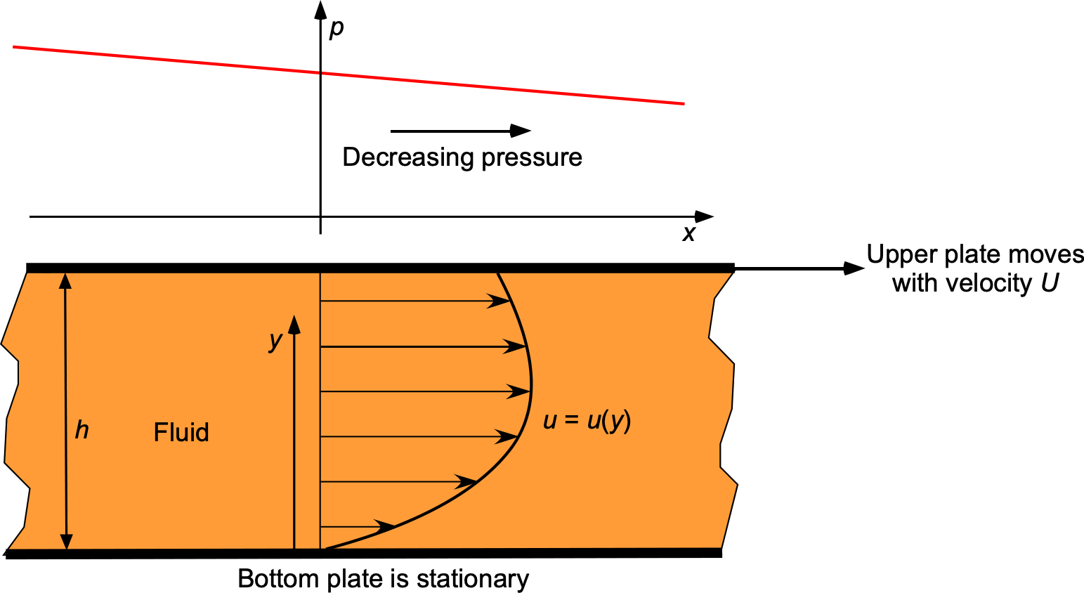
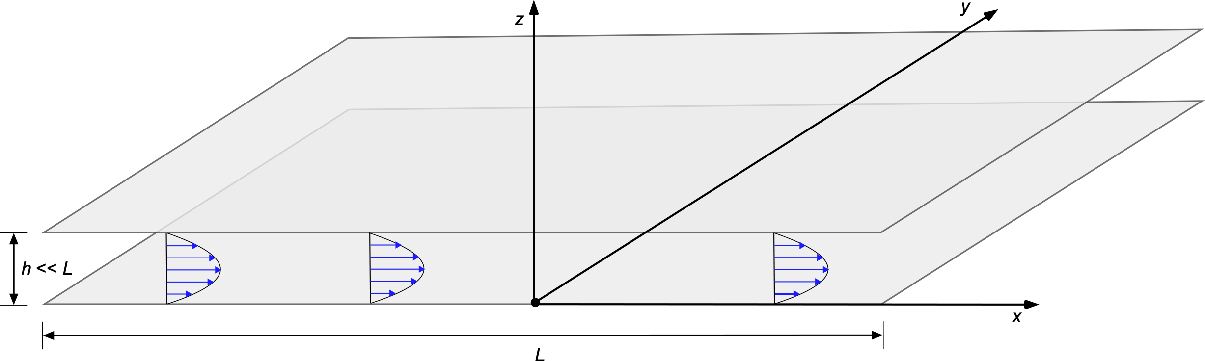
Consider a two-dimensional Stokes flow between two infinite, parallel plates located at  and
and  , as shown in the figure below. The lower plate at is stationary, while the upper plate at moves with a constant velocity
  in the
  -direction. A constant pressure gradient
  drives the flow along the -axis. The fluid is incompressible and viscous, and the Reynolds number is sufficiently low that inertial effects can be neglected.
 -direction; this gives a class of solutions known as Couette-Poiseuille flows.
The governing equations for steady, incompressible, two-dimensional flow in the – plane are the continuity and Navier-Stokes (momentum) equations. The continuity equation is
(20)
where and are the velocity components in the – and -directions, respectively. The momentum equations in the – and -directions are
(21) 
(22) 
Because the Reynolds number is small, the inertial terms involving can be neglected. The resulting Stokes equations are
(23) 
(24) 
If the flow is fully developed and unidirectional in the -direction, then  ,
,  , and
, and
(25) 
so the continuity equation is automatically satisfied. The -momentum equation simplifies to
(26) 
which leads to the second-order ordinary differential equation
(27) 
Integrating twice with respect to , the general solution is
(28) 
The boundary conditions are  and
and  . Applying gives
  , and applying gives
(29) 
so
(30) 
Substituting back into the general solution gives the final velocity profile as
(31) 
which may be rearranged as
(32) 
and this simplifies to
(33) 
showing explicitly the linear shear and parabolic pressure-driven contributions, i.e.,
(34) 
This is the velocity distribution for a combined pressure-driven and shear-driven (also called Couette-Poiseuille) flow between two parallel plates. Special cases include: 2. Pure Couette flow where  , resulting in a linear velocity profile. 2. Pure Poiseuille pressure-driven flow with
  , resulting in a parabolic profile symmetric about
  . Representative examples are shown in the figure below, which illustrate the behavior of Stokes flow between two infinite parallel plates under combined shear and pressure-driven conditions.
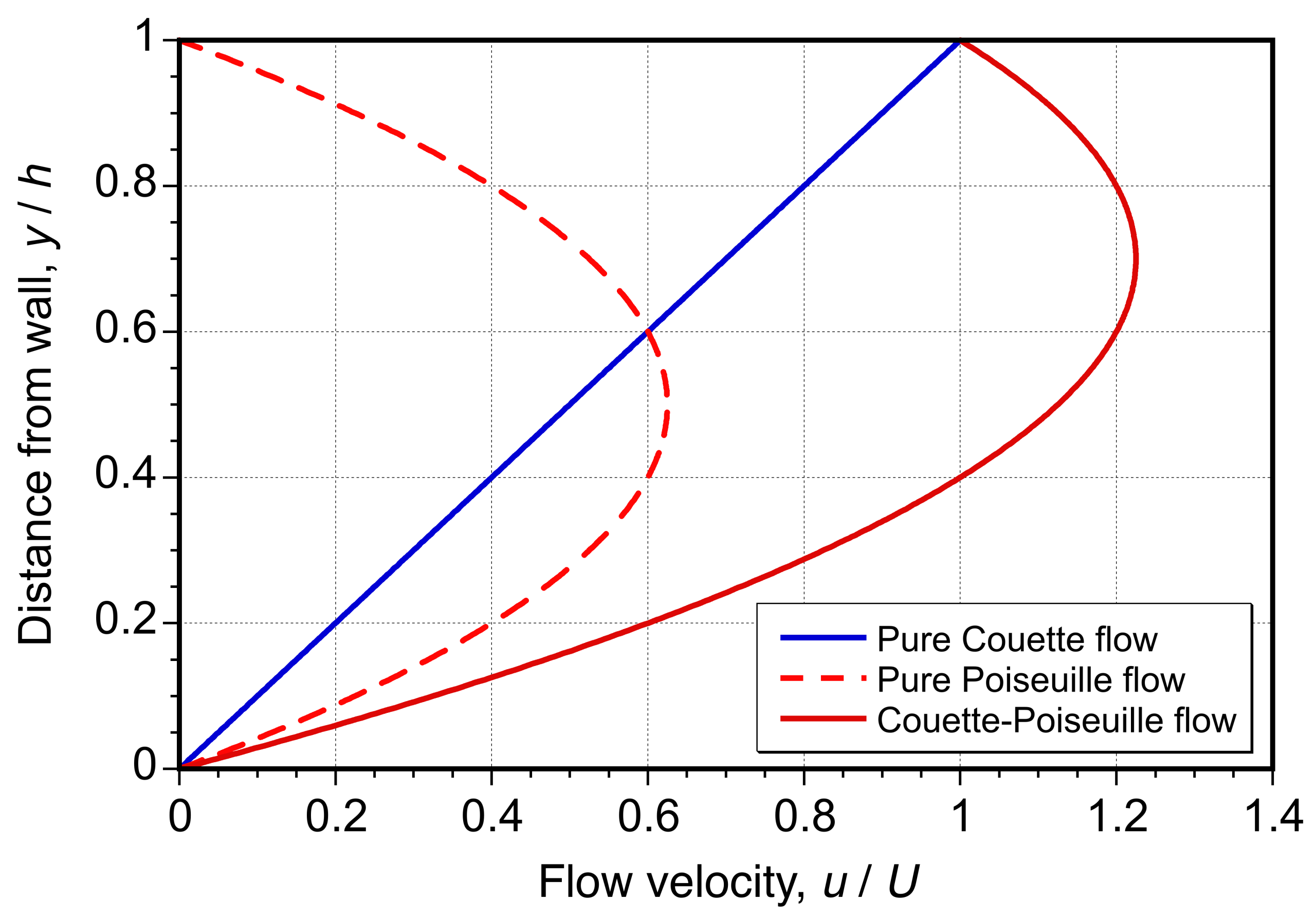
In pure Couette flow, which is driven solely by the motion of the upper plate, the velocity varies linearly across the gap. In contrast, pure Poiseuille flow, driven by a pressure gradient, exhibits a symmetric parabolic profile with the maximum velocity at the midplane. The combined Couette-Poiseuille flow is a linear superposition of these two effects, a valid process in any Stokes flow, resulting in a profile that combines the parabolic curvature of pressure-driven flow with the shear imposed by the moving wall. The maximum velocity shifts upward from the midplane because of the plate motion, and the profile illustrates how viscous forces distribute momentum across the space in low Reynolds number conditions.
Check Your Understanding #1 – Couette-Poiseuille flows
A viscous fluid flows steadily between two infinite, horizontal plates separated by a distance of  =1 cm. The bottom plate is stationary, while the top plate moves to the right with speed = 1 m/s. A constant pressure gradient
  is also applied to drive the flow. The dynamic viscosity is = 1 Pa s. Determine the value of that would cause the fluid velocity at the midplane
  2 to be zero. What does this result tell you about the balance of shear and pressure effects?
Show solution/hide solution.
The velocity profile for a combined Couette-Poiseuille flow is
![\[ u(y) = \underbrace{\frac{U}{h} y}_{\text{linear shear}} + \underbrace{\frac{1}{2\mu} \left( \frac{dp}{dx} \right) y(y - h)}_{\text{adverse pressure term}} \]](https://eaglepubs.erau.edu/app/uploads/quicklatex/quicklatex.com-1b0d46cf1c8231cd9b5f646e077f971a_l3.svg "Rendered by QuickLaTeX.com")
The required condition is that  , which means that the net velocity vanishes at mid-height, indicating a balance between wall-driven shear and pressure-driven flow reversal. Substituting gives
![\[ 0 = \frac{U}{h} \, \frac{h}{2} + \frac{1}{2\mu} \left( \frac{dp}{dx} \right) \, \frac{h}{2} \left( \frac{h}{2} - h \right) \]](https://eaglepubs.erau.edu/app/uploads/quicklatex/quicklatex.com-7d1c3fe50bcaba87c5534d015d0e1e26_l3.svg "Rendered by QuickLaTeX.com")
and on rearrangement then
![\[ 0 = \frac{U h}{2} - \frac{1}{8\mu} \left( \frac{dp}{dx} \right) h^2 \]](https://eaglepubs.erau.edu/app/uploads/quicklatex/quicklatex.com-c35f81f7d5c5fe199cb4c9ca9ef6efe2_l3.svg "Rendered by QuickLaTeX.com")
Solving for gives
![\[ \frac{dp}{dx} = \frac{4\mu U}{h} \]](https://eaglepubs.erau.edu/app/uploads/quicklatex/quicklatex.com-055cc48c6cc40d30ff9d466a322ca679_l3.svg "Rendered by QuickLaTeX.com")
Substituting the given numerical values, i.e.,  ,
,  , and
, and  , gives
![\[ \frac{dp}{dx} = \frac{4 \times 1 \times 1}{0.01} = 40{,}000\,\text{Pa/m} \]](https://eaglepubs.erau.edu/app/uploads/quicklatex/quicklatex.com-6f009207a234920a7e14a1dcc7b6b09a_l3.svg "Rendered by QuickLaTeX.com")
This pressure gradient is adverse, meaning pressure increases in the flow direction. It precisely cancels the forward Couette flow at the midpoint , so the new velocity there becomes zero, indicating a flow reversal in the lower half. This example illustrates how viscous and pressure forces can balance in creeping flows to produce internal stagnation and reverse flow, even when one boundary condition favors forward motion.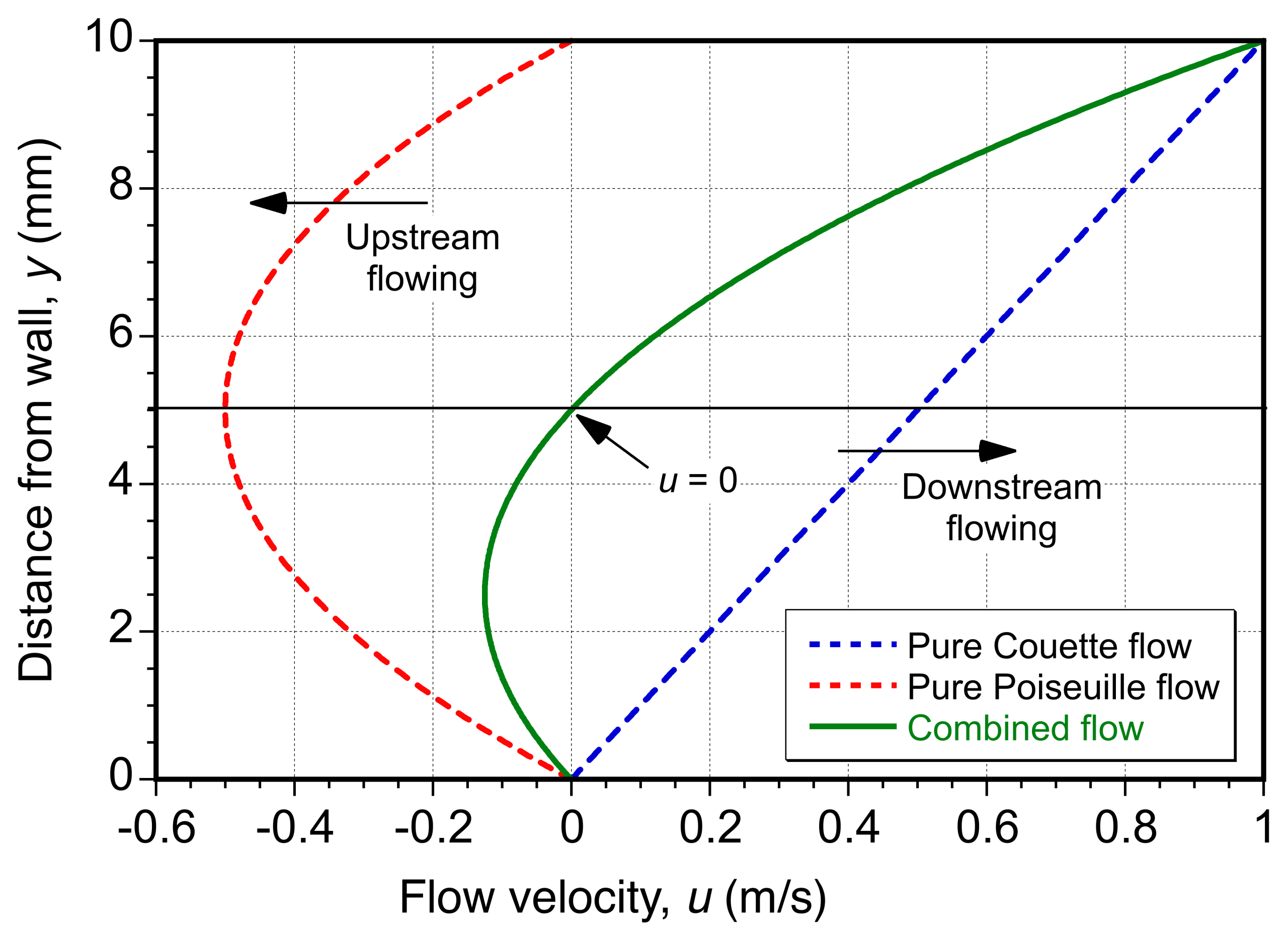
Poiseuille Flow in a Rectangular Channel
For internal flow through non-circular ducts, the concept of hydraulic diameter is often used for turbulent flows, but this approach does not accurately reproduce the laminar flow resistance and pressure drop through a rectangular channel. In this case, an analogous role is played by another correction factor that modifies the parallel-plate Poiseuille law to account for the additional viscous drag from the side walls.
As previously shown for infinitely long parallel plates of spacing and width  , the fully developed laminar volumetric flow rate for Poiseuille flow with a given pressure gradient is
(35) 
However, in a true rectangular channel, the viscous drag on the two side walls reduces the flow rate slightly. Solving Stokes’ equation with no-slip on all four walls gives the same equation structure but with a shape or aspect ratio correction factor  , i.e., now the flow rate is
(36) 
where the aspect ratio of the channel is  , and where for a uniform pressure gradient
  . This correction factor can be shown theoretically to be
(37) 
For practical use, however, the trigonometric  term is inconvenient, so an algebraic approximation is usually used, i.e.,
(38) 
Notice that for very wide channels where  , then
  and the classic Poiseuille parallel-plate formula for
  is recovered. For moderate aspect ratios,
  , reflecting the added viscous resistance of the side walls.
Hele-Shaw Flow
Hele-Shaw flow (after Henry Hele-Shaw) refers to the pressure-driven motion of a viscous fluid confined between two parallel flat plates that are separated by a narrow gap. Consider a steady, incompressible Newtonian flow in a thin gap between parallel plates located at  = 0 and
  , with
  as a characteristic in-plane length scale, as shown in the figure below. This geometry constrains fluid motion in the gap direction and produces a parabolic velocity distribution across the gap thickness. The Stokes equations apply to this flow, i.e.,
(39) 
together with no-slip and no-penetration on both plates. In a narrow gap, the pressure is uniform across the thickness to a leading order, so  , and the dominant viscous terms in the in-plane balances come from the second derivatives in . Retaining the dominant terms gives the pressure/shear component balances as
(40) 
where  are the in-plane velocity components, is the pressure, and is the coordinate normal to the plates. Because only in-plane pressure gradients drive the motion, the hydrostatic pressure in the direction can be neglected. The third relation above, therefore, shows that the pressure is independent of .
Integrating the first two equations twice with respect to and applying the no-slip boundary conditions at = 0 and gives
(41) 
This result shows that there is a parabolic velocity distribution across the gap, closely analogous to Poiseuille flow between two flat plates. The depth-averaged in-plane velocity is then obtained by integrating across the gap thickness and dividing by , i.e.,
(42) 
This latter relation shows that the average velocity is directly proportional to the pressure gradient, with a factor  , which is analogous to Darcy’s law[4] for flow through a porous medium; see the chapter on fluid properties. Therefore, the factor is equivalent to. permeability factor.
Conservation of mass requires that the averaged velocity field be divergence-free, i.e.,
(43)
Substituting the depth-averaged relation for shows that the pressure must satisfy Laplace’s equation, i.e.,
(44) 
when the spacing between the plates is uniform. Therefore, the pressure field in a Hele-Shaw flow is harmonic. The averaged velocity can also be expressed as the gradient of a potential, i.e.,
(45) 
so the flow is mathematically identical to two-dimensional potential flow, even though it arises from viscosity and is not irrotational. This correspondence seems contradictory and, in some sense, a paradox, but it provides a powerful analogy and explains the widespread use of Hele-Shaw flows as canonical models in fluid mechanics, including applications in flows through porous media and as approximations for shallow microfluidic channels.
It is important, however, to distinguish between the averaged two-dimensional description and the actual three-dimensional viscous flow in the gap. The velocity components of the full three-dimensional gap flow are
(46) 
so the vorticity is  , i.e., in terms of the components
(47) ![\begin{eqnarray*} \gamma_{x} & = & \frac{\partial w}{\partial y} - \frac{\partial v}{\partial z} = 0 - \left( -\frac{1}{2\mu}\,\frac{\partial p}{\partial y}\,(2 z - h) \right) = \frac{1}{2\mu}\,\frac{\partial p}{\partial y}\,(2 z - h) \\[6pt] \gamma_{y} & = & \frac{\partial u}{\partial z} - \frac{\partial w}{\partial x} = 0 -\frac{1}{2\mu}\,\frac{\partial p}{\partial x}\,(2 z - h) = -\frac{1}{2\mu}\,\frac{\partial p}{\partial x}\,(2 z - h) \\[6pt] \gamma_{z} & = & \frac{\partial v}{\partial x} - \frac{\partial u}{\partial y} = -\frac{1}{2\mu}(z^{2}-h z)\left(\frac{\partial^{2}p}{\partial y \partial x} - \frac{\partial^{2}p}{\partial x \partial y}\right) = 0 \end{eqnarray*}](https://eaglepubs.erau.edu/app/uploads/quicklatex/quicklatex.com-52a2ac63cbe36bed796228a427317c62_l3.svg "Rendered by QuickLaTeX.com")
noting that for any smooth pressure field then  , and so
  = 0. Therefore, the actual three-dimensional Hele-Shaw flow is viscous and rotational with nonzero
  and
and  (except at
  ), while vanishes identically. The depth-averaged in-plane vorticity components satisfy
(48) 
so the averaged in-plane flow is irrotational, and it allows the use of the potential function,  , as given above. The mathematical equivalence is therefore to two-dimensional potential flow for the depth-averaged field, even though the underlying three-dimensional motion is viscous and rotating. Therefore, Hele-Shaw’s method gives experimentalists a means of simulating a diffusive flow without the burden of using real porous materials, as well as a practical method of demonstrating potential flows in a laboratory setting; see here for a demonstration.
Stokes’ First and Second Problems
Stokes’ First Problem (impulsively started flat plate) was formulated as a canonical case of how momentum diffuses into a quiescent viscous fluid. Stokes’ Second Problem (oscillating plate) arose from Stokes’ interest in the fluid damping of pendulums and precision instruments. For this problem, the velocity disturbance was shown to be confined to a viscous penetration zone adjacent to the wall (the Stokes layer). Both problems allow exact analytical solutions, making them standard test cases in fluid mechanics and valuable tools for validating CFD solutions.
Stokes’ First Problem
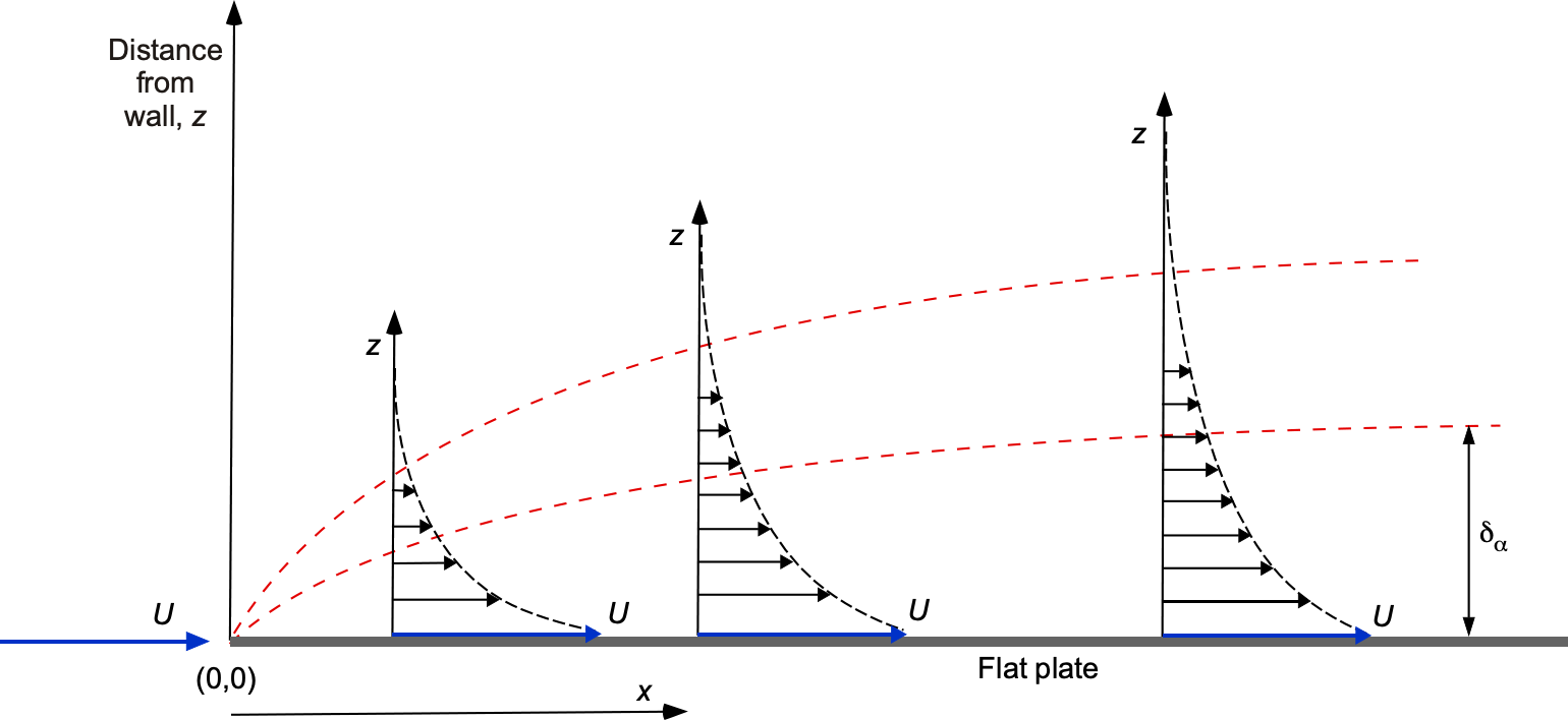
Consider a viscous, incompressible fluid occupying the half-space  . At
. At  , an infinite plate at
  is impulsively set into motion with constant speed in the -direction, as shown in the figure below. The initial and boundary conditions are
(49) 
The unsteady form of Stokes’ equation is
(50) 
Because the motion is unidirectional and there is no pressure gradient, the governing equation reduces to
(51) 
where  is the kinematic viscosity. Stokes assumed a dimensionless similarity variable of the form
(52) 
Notice that
(53) 
and
(54) 
Therefore, the governing partial differential equation in Eq. 51 now becomes an ODE in terms of the similarity variable, i.e.,
(55) 
which has the solution
(56) 
where  is the error function and
  and are constants. From the boundary condition
  then
then  and hence
  . Also, because
  then
then  and because
  , then
  . Therefore,
(57) 
where  is the complementary error function, and the velocity profile in the flow above the plate becomes
(58) 
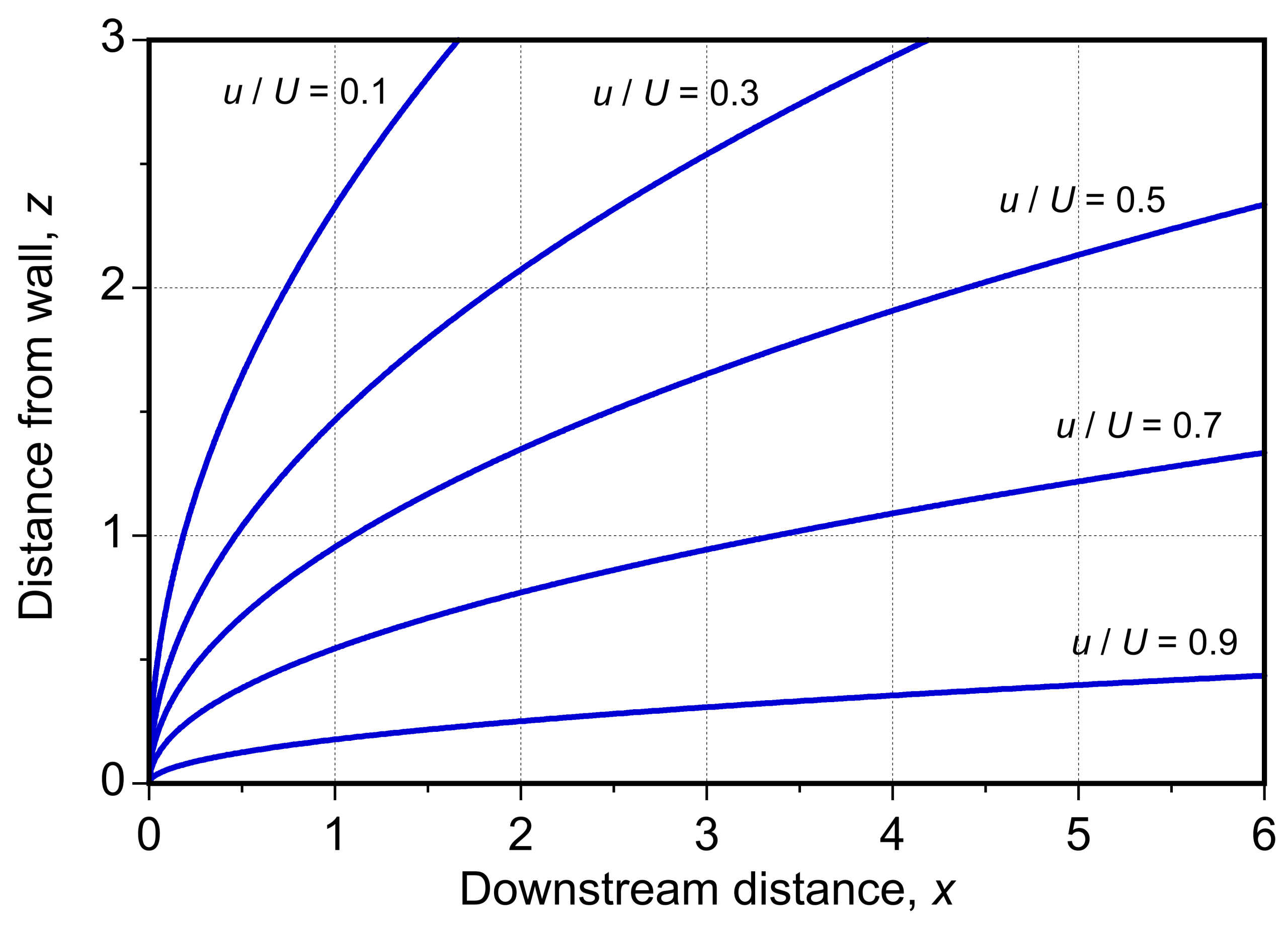
 is plotted versus downstream distance.
This solution shows that the disturbed layer thickness away from the plate grows diffusively, i.e.,  . A precise thickness may be defined by using a velocity threshold
  at
at  (
( ), i.e.,
(59) 
giving
(60) 
For example, with  then
then  .
.
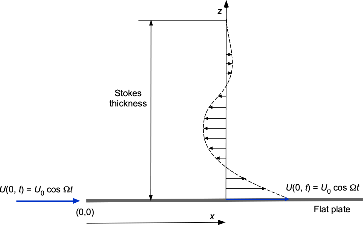
Stokes’ Second Problem
Now consider a related unsteady flow problem where the plate at  oscillates harmonically with velocity
  while the fluid at infinity remains at rest, i.e.,
  , as shown in the figure below.
Again, the governing flow equation is
(61) 
Because the forcing is periodic in time, Stokes used a harmonic solution of the form
(62) 
Differentiating gives
(63) 
and substitute into the governing equation to obtain
(64) 
which gives an ODE in terms of the complex amplitude, i.e.,
(65) 
Solving this constant coefficient ODE and selecting the decaying branch gives
(66) 
with the disturbed layer thickness, or Stokes layer, as it is called, being given by
(67) 
The boundary condition at the plate fixes the amplitude, i.e.,
(68) 
Taking the real part gives the velocity field as
(69) 
which decays exponentially above the surface and where the phase angle is  .
.
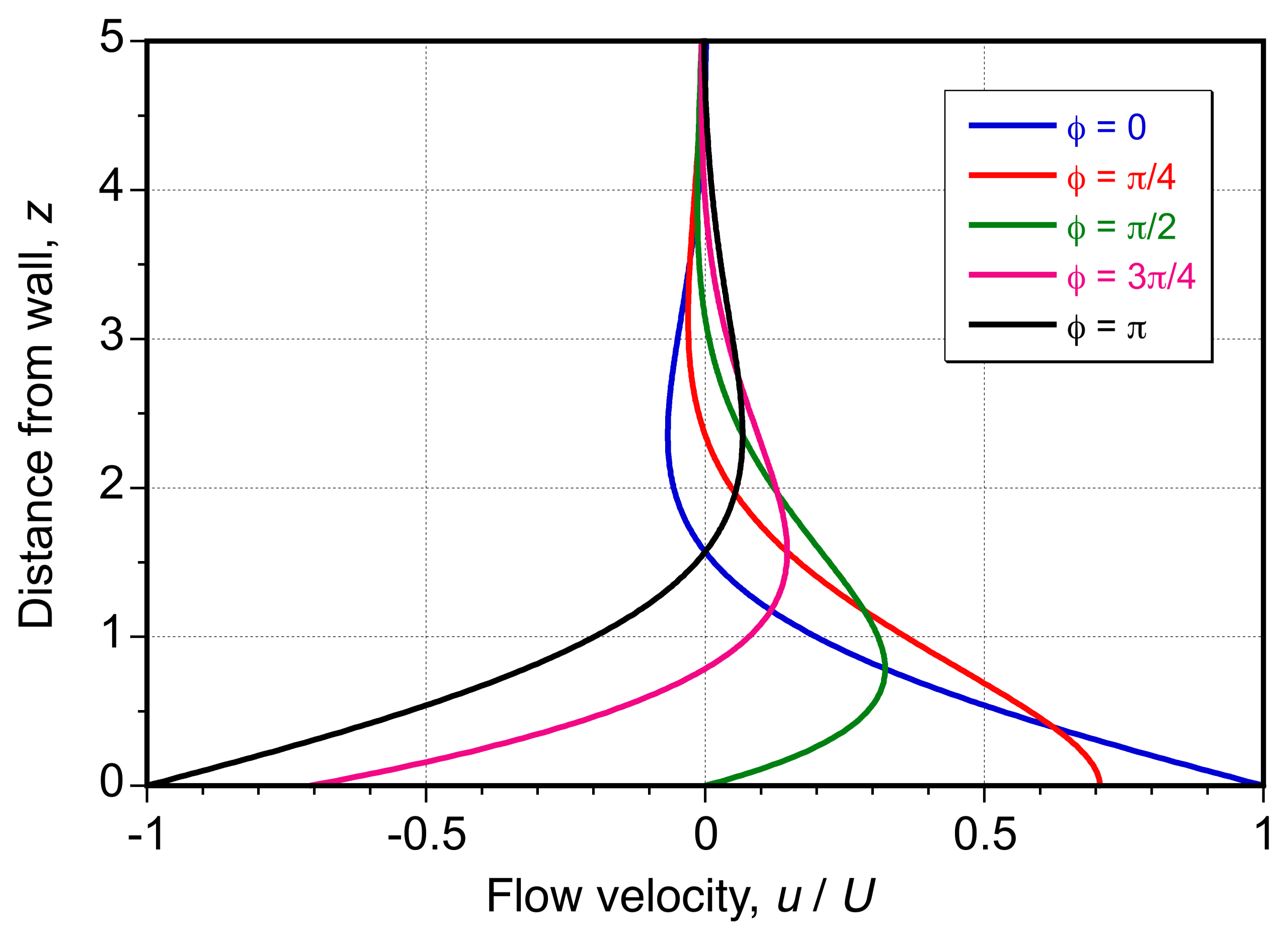 , while the flow lags the plate in terms of phase angle by
  .
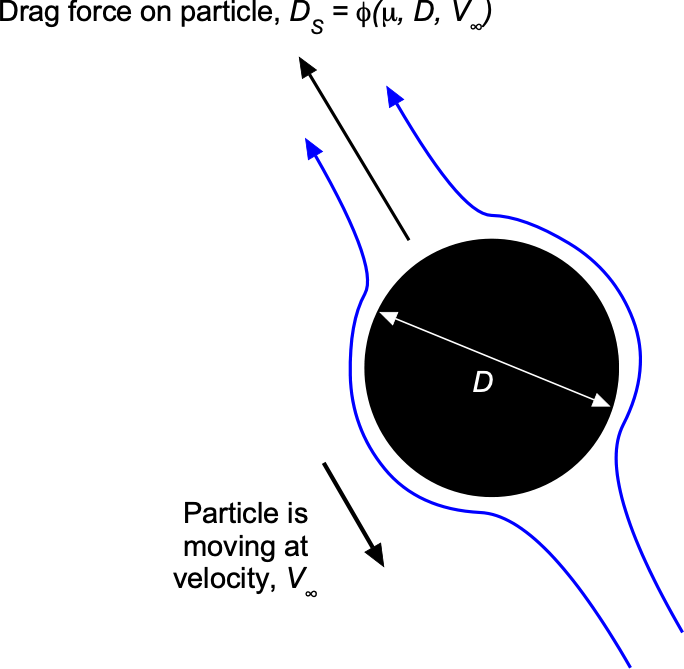
.Stokes’ Drag Law for Spheres
George Stokes established a foundational result for the drag force  on a spherical particle moving through a viscous fluid at a constant velocity
  in the Stokes flow regime. For very low Reynolds numbers, where inertial effects are negligible, the drag force is given by
(70) 
where is the viscosity,  is the sphere’s radius (
 ), and is the velocity of the particle relative to the fluid. This relationship, known as Stokes’ drag law, is derived based on the balance of viscous forces acting on the sphere and has been experimentally validated.
Using the Buckingham Pi method, the drag force can be expressed as
(71) 
In this case, represents the drag force with dimensions of  , has dimension
  , has dimensions
  , and is the velocity of the sphere with dimensions
  . The number of variables is
  , and the number of fundamental dimensions (
 , , and
  ) is
) is  . Therefore, using the Buckingham
  method, the number of dimensionless groups is
  .
.
This dimensionless group is formed as
(72) 
To make dimensionless, the dimensions of each variable are substituted, giving
(73) ![\begin{equation*} [\Pi] = 1 = \rm M^0 L^0 T^0 = (\rm M L T^{-2}) (\rm M L^{-1} T^{-1})^\alpha (\rm L)^\beta (\rm L T^{-1})^\gamma \end{equation*}](https://eaglepubs.erau.edu/app/uploads/quicklatex/quicklatex.com-5c66500320dba11153bdb708388041f0_l3.svg "Rendered by QuickLaTeX.com")
Equating the exponents of , , and on both sides yields  ,
,  , and
, and  . Solving these simultaneous algebraic equations gives
  ,
,  , and
, and  . Substituting these numerical values into Eq. 73 gives
(74) 
Because is dimensionless, the drag force can be expressed as  , where
  is a dimensionless constant. Experiments and other theories have determined that
  for a sphere, leading to Stokes’ drag law, i.e.,
(75) 
This latter result is valid for very low Reynolds numbers (), where viscous forces dominate over inertial forces, although its limits of applicability seem to extend to  . In general, for any body shape of characteristic length in Stokes flow, the drag can be written as
(76) 
where depends on the body shape.
Drag Coefficient
The drag coefficient  for a sphere in Stokes flow can be derived from the conventional drag force expression by normalizing the drag force by the freestream dynamic pressure and the sphere’s cross-sectional area, i.e.,
  . This drag coefficient is defined as
(77) 
Substituting Stokes’ drag law into this definition yields
(78) 
where  is the Reynolds number for the sphere. This latter relationship illustrates that the drag coefficient increases as the Reynolds number decreases, emphasizing the dominance of viscous forces at low Reynolds numbers. Alternatively, another form of the drag coefficient for Stokes flow can be written as
(79) 
and so using Eq. 75 then  for a sphere.
Theoretical Derivation of Stokes’ Drag Law
It has been shown that for low Reynolds numbers (creeping flow), the N-S equation simplifies to
(80)
which represents a balance between pressure forces and viscous forces. In spherical coordinates  centered on the spherical particle, the velocity field is expressed as
(81) 
where  and
and  are the radial and tangential velocity components, respectively. This problem has azimuthal symmetry, so the dependency on is removed.
The boundary conditions for the flow are:
- At the surface of the sphere where
 , then
  , where is the velocity of the particle through the flow.
 - Far from the surface where
 , then
  .
.
By solving the Stokes flow equations under these boundary conditions, the velocity field components are found to be
(82) 
(83) 
These results show that the velocity field does not depend on the viscosity, , even though the drag depends on because the shear stresses depend on the velocity gradients.
Notice that by substituting into Eq. 82, then
(84) 
i.e., the radial velocity is zero, satisfying the surface’s flow tangency (no-penetration) condition. Also, is substituted for the tangential flow component in Eq. 83 gives
(85) 
So, the tangential velocity is also zero at , i.e., the no-slip condition is satisfied.
The stress tensor components are required to compute the drag force on the sphere. The pressure, , acts inward and normal to the surface so that the total stress at the sphere’s surface is given by
(86) 
where  is the radial velocitiy gradient. If the velocity field at is substituted into the radial derivative, then
(87) 
The total drag force (pressure plus viscous) is obtained by integrating the stresses over the sphere’s surface. Therefore, the drag force is expressed as
(88) 
where  is the elemental surface area on the sphere. Substituting
  and integrating over
  (from 0 to
  ) and (from 0 to
  ) yields
(89) 
The surface integral can be separated into two parts:
- The azimuthal integral over from
 to , i.e.,
(90)

- The polar integral over from to , i.e.,
(91)

Using the trigonometric identity  , and the symmetry of the pressure term, the polar integral simplifies to
(92) 
because the pressure distribution is symmetric for and aft, as well as side to side, about the equators. For the viscous stress term, then
(93) 
and using the substitution  and so
  , gives
(94) 
Combining the results gives
(95) 
or in coefficient form
(96) 
This latter expression is called Stokes’ drag law. Once again, it applies only to a sphere moving through a viscous fluid at very low Reynolds numbers (), where inertial forces are negligible and viscous forces dominate.
Oseen Equations
The Oseen equations are an extension of the Stokes equations for creeping flows, which include minor inertial effects while remaining linear. They are particularly useful for analyzing flows around objects such as spheres or cylinders at low but finite Reynolds numbers.
The starting point is again the incompressible N-S equation, i.e.,
(97) 
For Oseen flow, it is assumed that the flow is steady, just as in Stokes flow, so . At low Reynolds numbers, inertial effects are minor compared to the viscous impacts. Additionally, a uniform far-field velocity  is assumed, where the flow has a constant velocity far from the object.
To simplify the convective term , the velocity can be re-expressed as
(98) 
where  is the disturbance velocity from the object. Substituting this expression into the N-S equation and linearizing the convective term results in the inertial term
  . The final Oseen equations then take the form
(99) 
Unlike the Stokes equations, which neglect all inertial terms and assume  , the Oseen equations include the linearized inertial term
  , extending their validity to Reynolds numbers of about 10.
For example, in the flow around a sphere, the Oseen solution for the velocity field becomes
(100) 
which can be compared with Eq. 82 for pure Stokes flow. For the radial component, then
(101) 
which can be compared with Eq. 83 for Stokes flow. At larger distances, i.e., , the velocity approaches the uniform far-field flow of , decaying as  , as opposed to the
  decay of the Stokes solution.
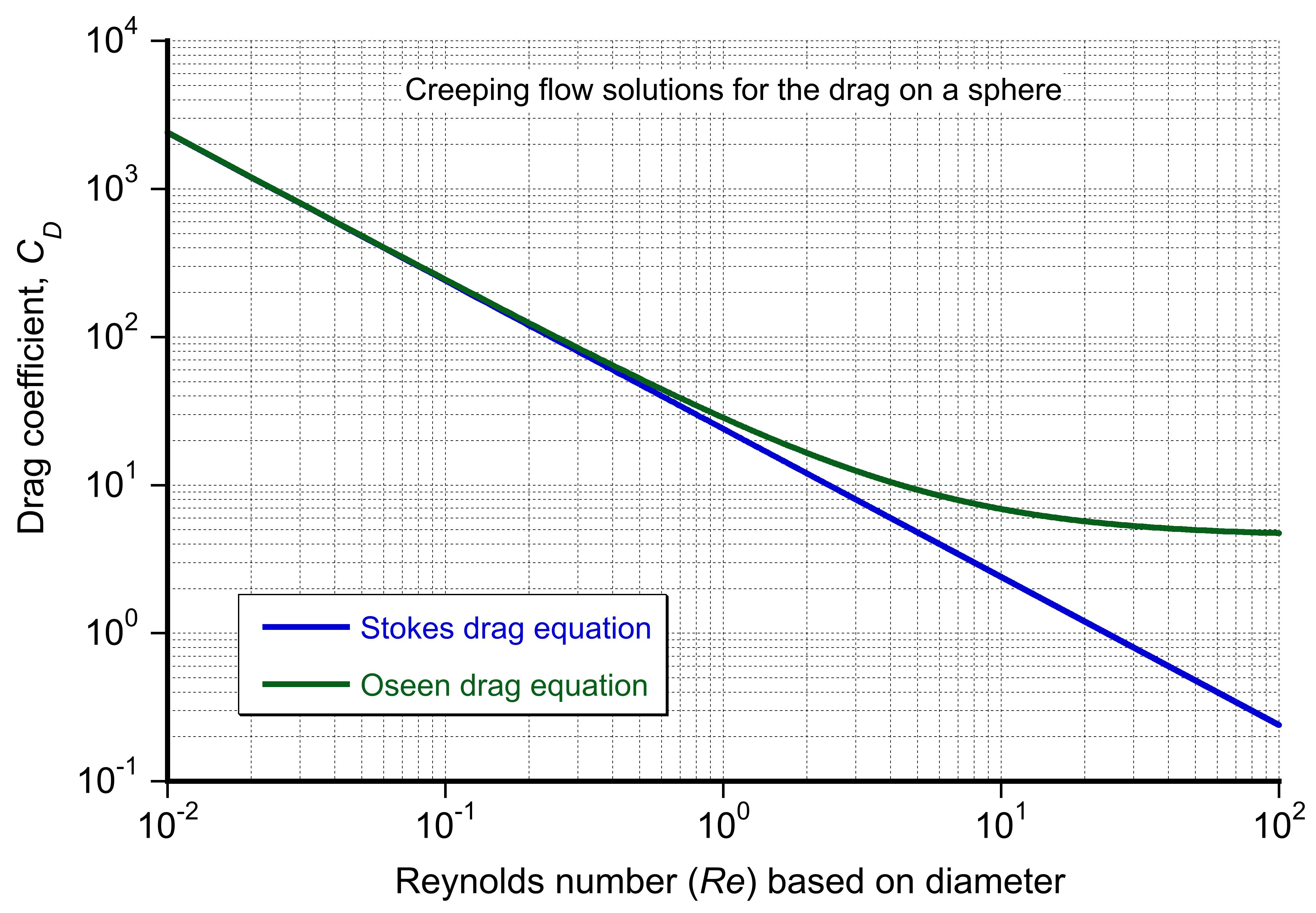
The resulting correction to Stokes’ drag law is given by
(102) 
where is the sphere’s radius, and the  term is the Reynolds number correction for weak inertial effects. In this case, the Stokes drag coefficient,
  for a sphere in creeping flow is
(103) 
The conventional drag coefficient, including the Oseen correction, is
(104) 
This latter result aligns with the creeping-flow behavior at low and includes the inertial correction. The results for both the Stokes and Oseen drag coefficients are shown in the plot below. The Oseen correction accounts for weak inertial effects, providing a more physically representative solution for slightly higher Reynolds numbers.
 , which the Oseen model can then replace.
The Oseen equations provide improved predictions for the flow and drag behavior at low but finite Reynolds numbers, typically below 100. They are especially useful for studying flows around objects, wake formation, and flow through porous media. For example, Oseen’s analysis shows that inertial effects lead to streamlines that deviate slightly from those in purely viscous Stokes flow. However, the Oseen equations are limited to low Reynolds numbers where linear inertial effects can be linearized. At higher Reynolds numbers, the solutions to the N-S equation are more difficult because of the need to solve for both nonlinear inertial and viscous effects.
Check Your Understanding #2 – Why does a ball bearing fall so slowly in glycerin?
In Dr. Leishman’s classes, he does a demonstration where he drops a tiny steel ball bearing into a test tube filled with glycerin. He says it’s a demonstration of Stokes’ flow. You first expect the ball bearing to fall quickly because it’s made of steel, but to your surprise, it drifts slowly downward in the tube, almost hovering in place. How slow is it really, and can you predict the speed using Stokes’ flow fluid mechanics? The ball has a radius of = 0.5 mm. Assume the density of steel is  = 7,850 kg/m
 , the density of glycerin is
  = 1,260 kg/m, and the viscosity of glycerin at room temperature is = 1.5 Pa s. What might happen if Dr. Leishman used ketchup instead of glycerin?
Show solution/hide solution.
This example shows how dramatically viscosity can dominate over inertia at specific scales. Assuming the motion is slow enough that inertial effects are negligible, you decide that the classic Stokes flow result gives the terminal settling velocity. In equilibrium, the downward force from the weight of the ball,  , less the buoyancy force,
  , is balanced by the viscous drag on the ball,
  , i.e.,
![\[ W_b - B_b = D_{\mu} \]](https://eaglepubs.erau.edu/app/uploads/quicklatex/quicklatex.com-7db68705cc0b4d0e1137732a54b8f538_l3.svg "Rendered by QuickLaTeX.com")
The weight of the ball is
![\[ W_b = \varrho_s \left( \frac{4}{3} \pi \, a^3 \right) g \]](https://eaglepubs.erau.edu/app/uploads/quicklatex/quicklatex.com-38abf5201d03b5a21f5d005d4c12aff9_l3.svg "Rendered by QuickLaTeX.com")
and the upward buoyancy force is
![\[ B_b = \varrho_f \left( \frac{4}{3} \pi \, a^3 \right) g \]](https://eaglepubs.erau.edu/app/uploads/quicklatex/quicklatex.com-93c6a54cd438665d29ebc3e729e7d231_l3.svg "Rendered by QuickLaTeX.com")
Therefore, the net downward force is
![\[ W_b - B_b = \frac{4}{3} \pi \, a^3 \, g (\varrho_s - \varrho_f) \]](https://eaglepubs.erau.edu/app/uploads/quicklatex/quicklatex.com-2c69ab10a8ba3c8b913ae885fd71b5bb_l3.svg "Rendered by QuickLaTeX.com")
The Stokes drag on a sphere is given by
![\[ D_{\mu} = 6 \pi \, \mu \, a \, V_d \]](https://eaglepubs.erau.edu/app/uploads/quicklatex/quicklatex.com-6514e2681a2d8f447c31f91ce0275c3d_l3.svg "Rendered by QuickLaTeX.com")
so balancing forces gives
![\[ \frac{4}{3} \pi \, a^3 \, g (\varrho_s - \varrho_f) = 6 \pi \, \mu \, a \, V_d \]](https://eaglepubs.erau.edu/app/uploads/quicklatex/quicklatex.com-3b88c3a4f57e2d35864ced118c9ec1f7_l3.svg "Rendered by QuickLaTeX.com")
and solving for  gives
gives
![\[ V_d = \frac{2 a^2 \, g (\varrho_s - \varrho_f)}{9 \mu} \]](https://eaglepubs.erau.edu/app/uploads/quicklatex/quicklatex.com-21e5de9cbeb2c0d854ad393f6da4be51_l3.svg "Rendered by QuickLaTeX.com")
Substituting the known values gives
![\[ V_d = \frac{2 \times 0.0005^2 \times (7,850 - 1,260) \times 9.81}{9 \times 1.5} = 2.39 \times 10^{-3} \ \text{m/s}. \]](https://eaglepubs.erau.edu/app/uploads/quicklatex/quicklatex.com-327a44f7902afdc3fd88fd605940c9be_l3.svg "Rendered by QuickLaTeX.com")
This is a very low velocity of only 2.4 mm/s. At this rate, it would take about 60 seconds for the ball to fall to the bottom of the test tube, as observed in Dr. Leishman’s demonstration.
To check the assumption of Stokes flow, compute the Reynolds number, i.e.,
![\[ Re = \frac{\varrho_f \, V_d \, 2 a}{\mu} = \frac{1,260 \times 2.39 \times 10^{-3} \times 0.001}{1.5} = \frac{3.011 \times 10^{-3}}{1.5} \approx 2.0 \]](https://eaglepubs.erau.edu/app/uploads/quicklatex/quicklatex.com-d1c1b5afa92c05c1e0d3b46d32765b28_l3.svg "Rendered by QuickLaTeX.com")
Although slightly above the strict criterion, the Stokes solution is still valid. However, for improved accuracy, Oseen’s correction may be applied to the drag law, i.e.,
![\[ D_{\mu} = 6 \pi \, \mu \, a \, V_d \left( 1 + \frac{3}{8} Re \right) \]](https://eaglepubs.erau.edu/app/uploads/quicklatex/quicklatex.com-a964ec806ebac73ac558f0888ec8752d_l3.svg "Rendered by QuickLaTeX.com")
Substituting this into the force balance gives
![\[ \frac{4}{3} \pi \, a^3 \, g (\varrho_s - \varrho_f) = 6 \pi \, \mu \, a \, V_d + \frac{9}{2} \pi \, a^2 \varrho_f \, V_d^2 \]](https://eaglepubs.erau.edu/app/uploads/quicklatex/quicklatex.com-0e148b7e8ce343d4c6082131fa428526_l3.svg "Rendered by QuickLaTeX.com")
This is a quadratic equation in , which can be solved iteratively, starting with the Stokes value. The Oseen correction gives a new estimate, and repeating the process gives convergence to an improved value of
(105) 
This result shows that the original Stokes prediction slightly overestimated the descent velocity. The corrected Reynolds number is now
(106) 
indicating that nominally the flow remains in the Stokes regime.
What might happen if the glycerine is replaced by ketchup? Ketchup behaves as a yield-stress fluid, meaning it will not flow unless the applied stress exceeds a particular critical value. In practical terms, this means that a small steel ball placed in ketchup may not sink at all if its weight is insufficient to overcome this resistance. If the ball does move, its settling speed will not be uniform because it is a non-Newtonian fluid. With a larger ball, it may move slowly at first, then accelerate as the shear stress in the fluid around the ball increases. Try it!
Comparison of Stokes Flow & Potential Flow
Stokes (creeping) and potential flows may appear superficially similar, but they are distinct flow conditions that describe fluid behavior around bodies under different physical assumptions and conditions. Indeed, their characteristics, mathematical descriptions, and physical implications differ significantly. Creeping flow occurs at very low Reynolds numbers, i.e., , where viscous forces dominate and inertial effects are negligible. In contrast, potential flow represents an idealized, inviscid, and irrotational flow regime, where inertial forces dominate and viscous effects are ignored, i.e.,  . Potential flow solutions apply to high-Reynolds-number flows outside boundary layers.
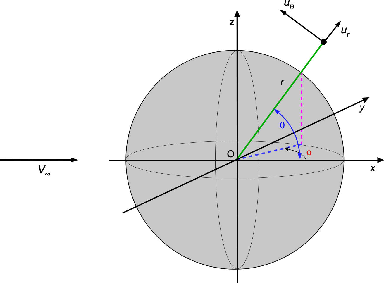
On the one hand, as previously shown, creeping flow is derived from the Stokes equations, which simplify the N-S equation by neglecting inertial terms. The velocity components for creeping flow are axisymmetric, so they depend only on the  and coordinates, i.e., referring to the figure below, then
(107) 
(108) 
Notice that these latter equations include terms proportional to  and
and  , reflecting the rapid reduction in viscous effects away from the surface.
On the other hand, potential flow is governed by the Laplace equation and is an inviscid, irrotational flow. In this case, the velocity components for potential flow are
(109) 
(110) 
In this case, the velocity components decay faster overall at a rate proportional to compared to creeping flow because of the absence of viscosity.
Streamlines About a Sphere
The figure below shows the predicted streamline patterns for Stokes flow (left) and potential flow (right) around a sphere. Not every streamline can be continuously solved on a finite grid, resulting in a few gaps in the solution, although these should not detract from the overall patterns. Comparing the results highlights several differences. While the streamline patterns may look qualitatively similar, the far-field effects differ markedly. Notice that in creeping flow, the inclusion of terms proportional to reflects the slower decay of viscous effects, which dominate at intermediate distances. However, that effect may not be visually apparent in the plots below.
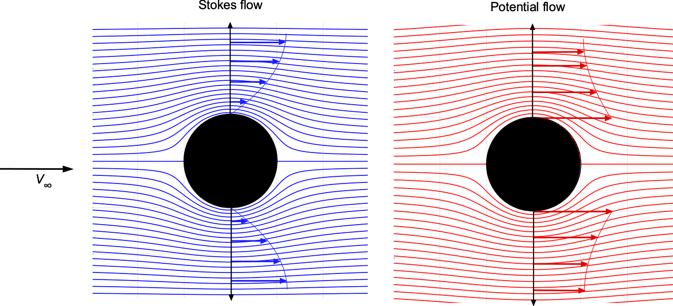
In potential flow, all velocity terms decay as , showing a faster reduction of the flow disturbance with distance. The absence of viscosity limits the spatial extent of the disturbance. The velocity near the sphere is slower than the freestream velocity everywhere, unlike potential flow, where velocities can exceed the freestream velocity in some locations. The velocity profile in potential flow is also distinct. Substituting into Eq. 109 gives
(111) 
Therefore, the radial velocity satisfied the flow tangency (no-penetration) condition. For the tangential velocity, then substituting into Eq. 110 gives
(112) 
Therefore, in potential flow at the sphere’s surface, the local velocity is  at its equator. In contrast, the velocity is zero everywhere on the surface in Stokes flow because of the no-slip condition.
Drag is also where the two flows differ. Potential flow predicts zero drag (d’Alembert’s paradox), i.e., no pressure drag and no viscous drag, so  , while creeping flow exhibits significant viscous drag, as given by
(113) 
As previously discussed, an alternative drag coefficient can be defined for creeping flow. The Stokes drag coefficient, for a sphere in creeping flow is
(114) 
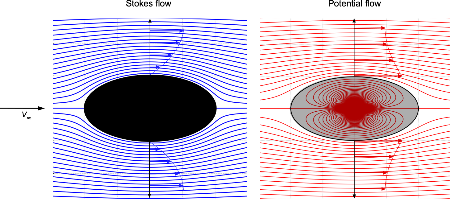
Flow Around a Two-Dimensional Ellipse
Unlike the sphere, solutions to Stokes flows around other bodies must be computed numerically. Consider the flow about a unit ellipse[5] as given by
(115) 
where and are the length fractions of the semi-major and semi-minor axes, respectively. The stream function  for Stokes flow satisfies the biharmonic equation
(116) 
The velocity components are
(117) 
The boundary conditions are:
- The flow tangency (no-penetration) boundary condition on the ellipse, i.e.,
 on the surface of the ellipse.
 - No-slip boundary condition on the ellipse, i.e.,
 .
. - Uniform flow is the far-field boundary condition, i.e.,
 , where is the freestream velocity.
The computational domain can be discretized using a uniform Cartesian grid for the numerical solution. The values of are initialized with the far-field condition . A finite-difference relaxation method can then be used to solve the biharmonic equation iteratively, i.e., using a centered-averaged stencil of the form
(118) 
where the index i runs in the x direction and j runs in the y direction. The boundary condition that is enforced on the ellipse at each iteration number  , and the process continues iterating until the solution converges to some acceptable numerical tolerance.
The results shown in the figure below appear reasonable, even though they were generated on a Cartesian grid, to illustrate the nature of this creeping flow. Again, notice how the effects of viscosity diminish away from the body, causing the streamlines to become more parallel to each other. The potential flow solution was also calculated numerically, with the interior of the ellipse’s surface (a dividing streamline) appearing as a doublet.
Particle Motion
It is essential to understand the fundamental principles governing particle motion in a fluid medium, which is a Stokes flow problem. When a solid particle is immersed in a flow, its movement is determined by the balance of drag, gravity, buoyancy, and inertia. A critical factor in this interaction is the time required for the particle motion to respond and adjust its velocity in response to changes in the surrounding fluid flow. This response time depends on the particle’s size, density, and the viscosity of the carrier fluid. Gaining insight into how particles respond to flow fluctuations is vital for accurately predicting their trajectories and behaviors in various applications.
Stokes Number
The Stokes number,  , is a dimensionless parameter that characterizes a solid particle’s behavior in a carrier flow. It is defined as the ratio of the particle relaxation time to a characteristic flow time scale
  , such that
(119) 
Here, represents the time scale over which significant changes in fluid velocity occur. This timescale is often associated with the most significant flow structures in the system, such as vortices. The Stokes number determines how well particles follow the fluid flow, which is essential in many applications.
Particle Relaxation Time
Particle Image Velocimetry (PIV) is a widely used experimental technique for analyzing fluid flow by tracking the motion of small particles, known as “seed,” suspended in the fluid. These particles are assumed to follow the flow, accurately representing the velocity field; however, errors can occur. The ability of the seed particles to respond to changes in the fluid motion is usually measured by the particle relaxation time,  , which quantifies the time lag for a particle to catch up to the surrounding fluid’s velocity. The relaxation time is given by
(120) 
where  is the particle’s density. Smaller particles with lower densities or those in highly viscous fluids exhibit shorter relaxation times. The idea is shown in the figure below.
If  , the particle relaxation time is much smaller than the fluid time scale, allowing particles to follow the fluid motion closely. This is ideal for PIV applications because the particle trajectories faithfully represent the fluid’s velocity field. Conversely, when
  , the particle relaxation time is larger than the fluid time scale, causing the particles to lag behind rapid changes in the fluid velocity. In this case, the particles do not accurately track the fluid motion, leading to errors in the velocity field measurements.
Selecting appropriate particles for PIV experiments is critical to ensuring accurate flow analysis. The particles must be small enough to maintain but large enough to produce Mie scattering of the laser light illumination. Understanding the interplay between particle size, density, relaxation time, fluid time scales, and the Stokes number is crucial for optimizing PIV performance and accurately interpreting results in complex flow environments.
Particle Tracking
In new PIV experiments, prototypical flow problems can be used to estimate particle tracking errors for particles of different sizes and densities. The forces involved are weight, viscous drag, and buoyancy. In many cases, when using solid particles in a gas, the buoyancy force can be neglected. The equations governing the particle displacements,  , can be expressed as two first-order differential equations, i.e.,
(121) 
where is the flow velocity at a point and  is the particle velocity. In this equation, the particle response time can be expressed as
(122) 
where  is the Reynolds number of the particle and
  is its Stokes drag coefficient.
As given by Eq. 121, the particle equations of motion can be solved for a prescribed prototypical velocity field using numerical integration schemes. The discretized equations can be written as
(123) 
This discretized set of equations are “stiff” because the value of changes significantly with particle diameter, and higher-order backward difference methods must be used.
Brownout
While suspensions of solid or liquid particles in a carrier flow are often modeled as continuous media for practical purposes, they consist of discrete particles immersed in a continuous fluid, where interactions such as hydrodynamic forces and Brownian motion play a role. Depending on the scale and application, the dual-phase nature of the combined flow influences its behavior, requiring a balance between continuum approximations and discrete-particle modeling.
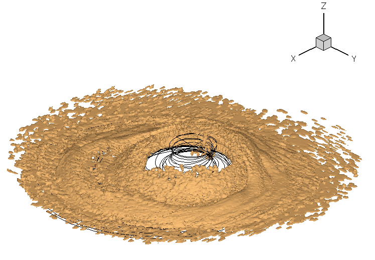
One relevant aerospace application involving Stokes flow is the problem of rotorcraft “brownout,” where a rotorcraft operating over loose sediment, such as sand, stirs up a large dust cloud, as illustrated in the figure below. This dust cloud causes numerous problems, including loss of visibility and spatial optical illusions for the pilot, as well as erosion of the rotor blades and turbine blades in the engines. Several interdependent particle mechanisms have been shown to affect brownout. Two-phase mechanisms such as saltation, particle bombardment, and sediment trapping by vortex flows are primary contributors to the overall formation of a brownout dust cloud. Particle motion can be described using the Stokes drag coefficient, which is typically calculated numerically to determine either individual particle trajectories or, more commonly, the trajectories of particle clusters.
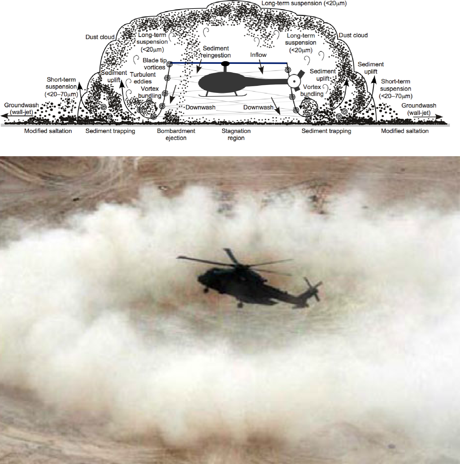
The many other interdependent factors involved in the brownout problem (including surface conditions, compactness, and moisture content, among others) suggest that modeling approaches can offer a way to gain physical insight into the fundamental parameters that influence the formation of these dust clouds. An example is shown in the figure below, which uses particle and particle-cluster tracking as previously described. Such models have value not only for their potential predictive capability but also for their ability to help understand the individual mechanisms contributing to sediment mobility and their significance in the brownout problem.
The difficulty in simulating brownout lies in the need for mathematical models to accurately resolve the detailed vortical structures and turbulent flow produced at the ground by the helicopter rotor’s wake, as well as the uplift and subsequent convection of billions of dust particles. It is essential to perform high-fidelity simulations to accurately predict the various particle mechanisms and the resulting optical characteristics and visibility within the dust cloud.
Particle Settling
Another classic application of Stokes flow is the steady settling of small, dispersed spherical particles in a carrier fluid, as shown in the schematic below. The theory of particle settling under Stokes flow provides critical insights into various sedimentation processes, particle dynamics in suspensions, and various industrial and environmental applications. An example would be settling the brownout dust cloud that was previously considered. Settling occurs under three primary forces acting on the particles, i.e., weight (gravitational force),  , the buoyancy force,
  , and the viscous drag force, . This is a problem in static force equilibrium, and the balance of these three forces collectively determines the settling rate of the particles.
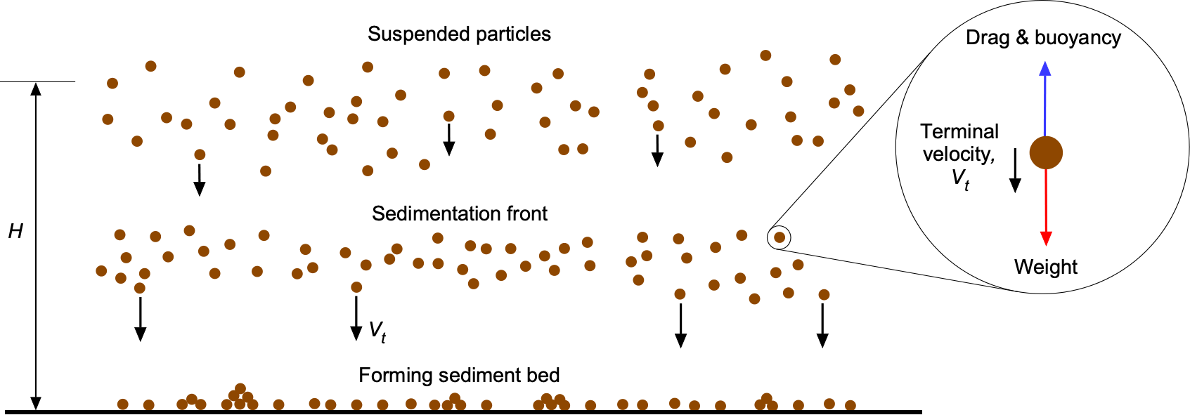
When any one particle reaches its terminal velocity  , the motion becomes steady, and the forces acting on the particle balance. This static force equilibrium can be expressed as
(124) 
Substituting the expressions for the individual forces, the gravitational force is given by the particle’s weight,  , where is the particle’s density, is its radius, and
  is the acceleration under gravity. The buoyancy force exerted by the displaced fluid is
  , where is the density of the fluid. Stokes’ drag law determines the viscous drag force, i.e.,
  . Combining these expressions, the force balance equation becomes
(125) 
Simplifying, the gravitational and buoyancy terms can be grouped, leading to
(126) 
Solving for the terminal velocity gives
(127) 
Notice that larger particles or more significant density differences lead to higher terminal velocities, while increased fluid viscosity reduces the settling rate. Tiny particles in the air have extremely low terminal velocities, meaning they can stay suspended almost indefinitely. The perpetual presence of volcanic dust in the atmosphere is a testament to this, as well as the time it takes for a brownout dust cloud to settle out.
Hindered Settling in Suspensions
The settling behavior of particles in suspensions depends significantly on the concentration of particles within the fluid. In dilute suspensions, where particle interactions are minimal, the settling time  for a particle to descend from an initial height
  can be described by the terminal velocity derived from Stokes’ flow. The settling time is given by
(128) 
where is the height, and and are the densities of the particle and fluid, respectively. In this scenario, each particle settles independently, and its individual properties and fluid characteristics govern the overall dynamics.
In concentrated suspensions, however, particle interactions significantly alter the settling behavior. These interactions include hydrodynamic effects, collisions, and disturbances in the local flow field, collectively hindering settling. As a result, the settling velocity decreases compared to the terminal velocity of a single particle in isolation. This phenomenon is known as hindered settling.
The hindered settling velocity  in concentrated suspensions can be described empirically as
(129) 
where is the particle volume fraction, representing the fraction of the suspension volume occupied by the particles, and is an empirical exponent that depends on the specific suspension system and the nature of particle interactions. The term  captures the reduction in velocity because of the increased particle concentration. As approaches 1, the velocity approaches zero, reflecting the complete suppression of settling in a densely packed system.
The relationship between hindered settling and particle concentration is critical in sedimentation, industrial slurry transport, and wastewater treatment applications. Understanding and modeling hindered settling provide insights into the behavior of particle-laden flows in both natural and engineered systems, helping to optimize processes involving suspensions of varying concentrations.
Taylor-Couette Flow
Taylor-Couette flow refers to the flow of a viscous fluid between two concentric cylinders, where one or both cylinders may rotate. This configuration is a classical problem in fluid mechanics, often studied to understand flow stability, transitions between flow regimes, and turbulence. The behavior of Taylor-Couette flow is determined by the geometry of the cylinders, their relative rotational speeds, and the properties of the fluid.
The radii of the inner and outer cylinders are denoted by  and
and  , respectively, while their rotational speeds are denoted by
  and
and  . Two dimensionless Reynolds numbers are defined to characterize the contributions of each cylinder to the flow, i.e.,
(130) 
where  is the kinematic viscosity of the fluid. These Reynolds numbers quantify the relative importance of inertial and viscous forces for each cylinder.
The Taylor number,  , is a dimensionless parameter that characterizes the onset of instability in the Taylor-Couette flow. It is defined as
(131) 
where  is an effective angular velocity that combines the rotational speeds of the two cylinders. The Taylor number represents the balance between the centrifugal forces that drive instability and the viscous forces that stabilize the flow.
At low Taylor numbers ( ), the flow is stable and laminar, characterized by a purely azimuthal velocity profile. The flow adheres to a steady, circular motion dictated by the boundary conditions at the cylinder surfaces. As the Taylor number increases and exceeds a critical value,
  , the flow becomes unstable from centrifugal forces, i.e., a body force effect. Axisymmetric vortices, known as Taylor vortices, emerge in the annular gap between the cylinders. These vortices appear as toroidal structures of alternating strengths stacked like donuts along the axis of the cylinders. Further increases in result in more complex flow patterns, including wavy vortices, modulated wavy vortices, and eventually, turbulent flow. These transitions depend on the relative rotational speeds of the cylinders and the gap width, i.e.,
  .
.
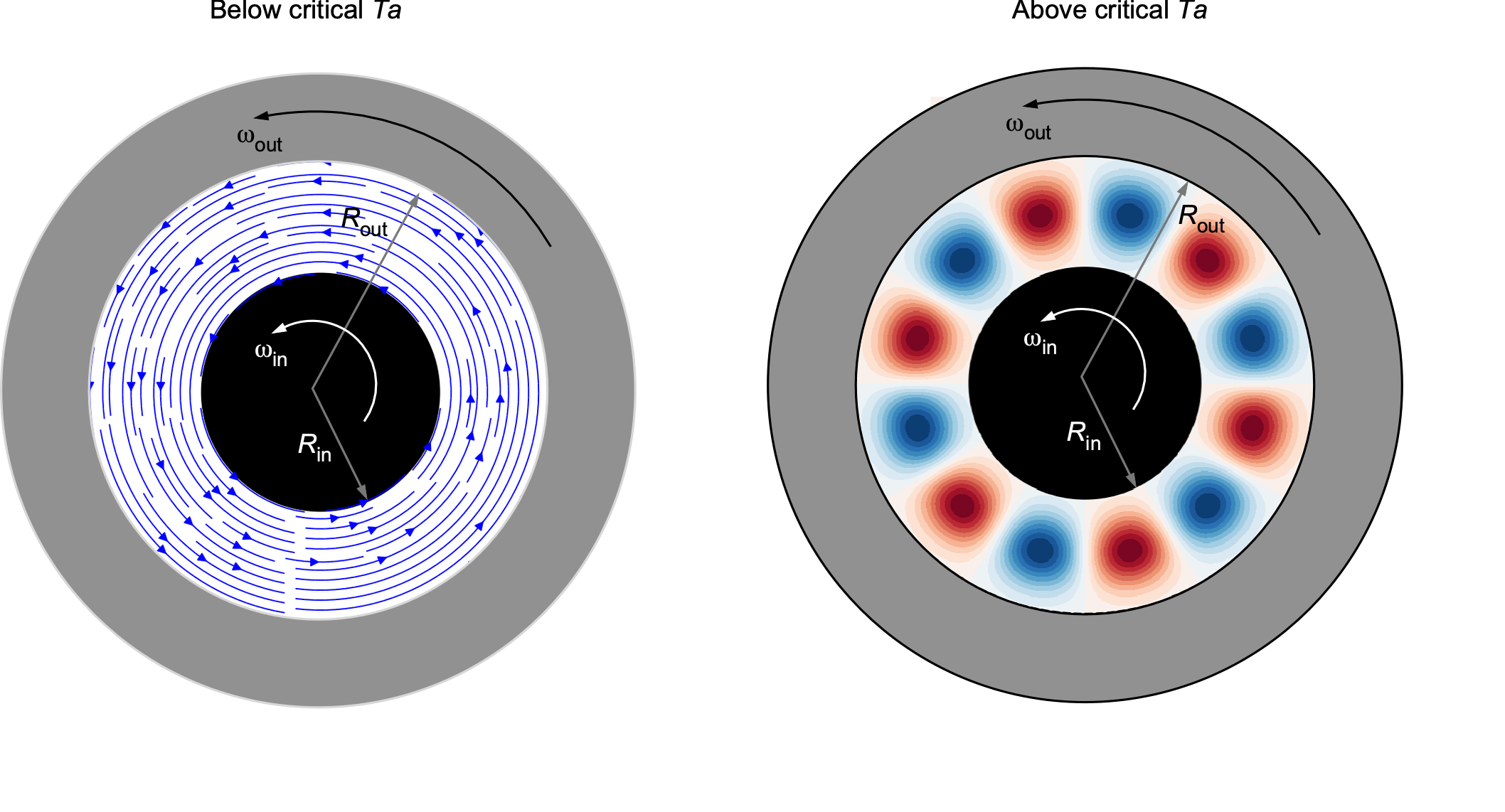
The study of Taylor-Couette flow remains integral to understanding fluid mechanics because of its well-defined geometry and the wide variety of flow phenomena it exhibits, from stable laminar motion to fully developed turbulence. However, Taylor-Couette flow has numerous applications in engineering, geophysics, and astrophysics in practice. It is relevant to mixing processes in chemical reactors, where controlled shear and turbulence enhance reaction rates. In turbulence and nonlinear dynamics research, Taylor-Couette flow provides a well-defined system for studying transitions between laminar flow, vortex structures, and chaotic behavior. In astrophysics, it models accretion disk dynamics, planetary formation, and other phenomena that are influenced by rotational flows.
Who were Taylor and Couette?
Maurice Couette (1858–1943) and Geoffrey Taylor (1886–1975) were pioneers in the field of fluid mechanics. Couette, a French physicist, is renowned for describing the motion of a viscous fluid between two concentric cylinders or parallel plates and inventing the Couette apparatus, a form of viscometer, to measure fluid viscosity. Taylor, a British physicist, extended the study to analyze the stability and transitions in fluid motion between rotating cylinders. Taylor’s discovery of Taylor vortices and his broader contributions to turbulence, instabilities, and wave propagation solidified his role as one of the most influential figures in the field of fluid dynamics. Specifically, their combined work laid the groundwork for a deeper understanding of complex shear-driven flows.
Non-Newtonian Viscous Fluids
Highly viscous non-Newtonian fluids exhibit shear-dependent viscosity, meaning their resistance to flow varies with the rate of deformation. Despite the complexity of their internal microstructures, many such non-Newtonian fluids can be effectively described using the empirical power-law model, i.e.,
(132) 
where  is the shear stress,
  is the shear rate,
  is the consistency index, and is the flow behavior index. This model generalizes the Newtonian behavior, which is recovered when
  and
and  . If
. If  , the fluid is shear thinning (pseudoplastic), with decreasing effective viscosity at higher shear rates. If
  , then the fluid is shear-thickening (dilatant), becoming more viscous as it is deformed more rapidly, as shown in the figure below.
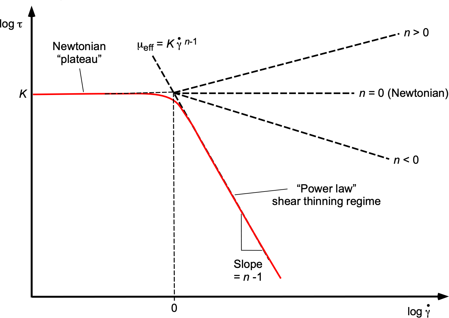
In the power-law model, the effective viscosity is given by
(133) 
The values of and are typically measured using rotational rheometers. While the power-law model breaks down at very low or very high shear rates, it is widely used to characterize creeping or slow viscous flows, where such nonlinearities are key to understanding fluid dynamics.
Non-Newtonian fluids arise in various applications of aerospace engineering, where the governing flows are typically viscous-dominated and controlled by rheology rather than inertia. For example, in propellant manufacturing, solid rocket grains are cast from concentrated suspensions of oxidizer in polymer binders, forming a shear-thinning slurry that can be represented by the power-law, where the viscous flow sets the distribution of particles and voids before curing. Gelled propellants, used in some missile and spacecraft systems, exhibit Bingham plastic behavior with a finite yield stress, described by
(134) 
where  is the yield stress and
  is the plastic (post-yield) viscosity, so their redistribution in tanks or under microgravity is controlled by viscous rather than inertial forces. During atmospheric re-entry, ablation of thermal protection materials produces the melting and movement of layers that are highly viscous and non-Newtonian in character; their slow flow is better captured by viscosity expressed in terms of a Carreau model, i.e.,
(135) 
where  is the zero-shear viscosity,
  is the infinite-shear viscosity, and
  is the characteristic relaxation time. In all three applications, the flow is viscous-dominated, and the non-Newtonian behavior arises from the material’s stress-dependent viscosity and yield behavior.
Kelvin’s Pitch Glacier Experiment
In 1887, Professor William Thompson (Lord Kelvin) conducted a demonstration to show that certain materials, though seemingly solid, can behave like fluids over long periods. He set a block of bitumen pitch into the top step of a desktop-scale wooden staircase. Although the pitch initially appeared solid at the top step, it slowly sagged under gravity and crept toward the lower steps, a process that has continued over many years. It still flows today and is known as Kelvin’s pitch glacier experiment. It is kept at the Hunterian Museum at the University of Glasgow, where Kelvin was the head of the Natural Philosophy Department.
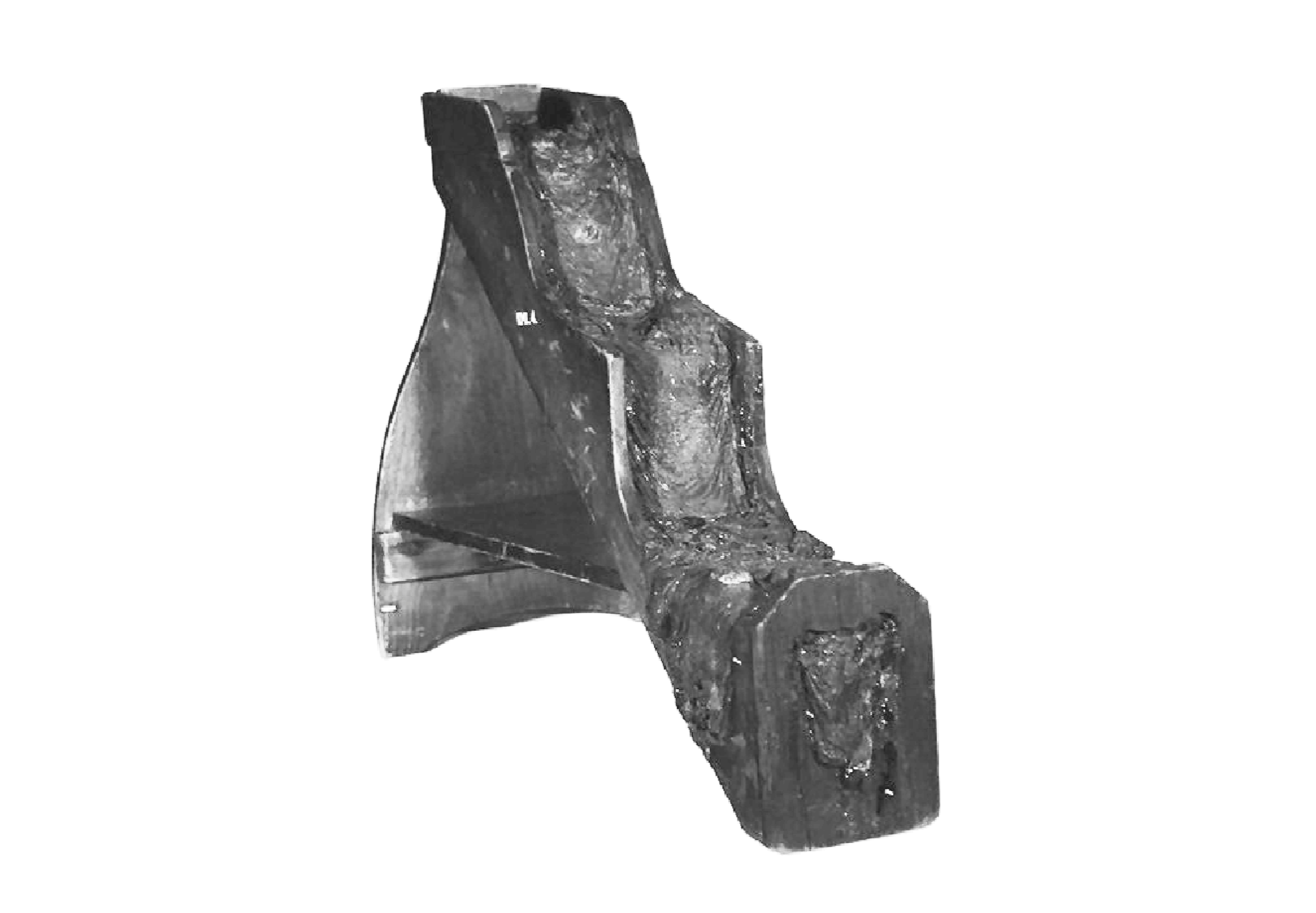
Pitch, often just referred to as tar or asphalt, is a highly viscous fluid, with a dynamic viscosity on the order of  to
to  Pa s. Kelvin used the behavior of pitch as an analogy for glacier flow, noting that glacial ice, though solid in appearance, also flows slowly downhill under its own weight. Kelvin’s experiment, therefore, serves as a physical demonstration of a driven shear flow in a highly viscous non-Newtonian medium.
The basic fluid mechanics can be described by assuming a block of pitch of thickness lying on a slope of angle  , as shown in the figure below. The block will eventually deform under gravity and flow very slowly downhill. Initially, nothing moves, but as gravity acts, shear stresses build up, causing the pitch to flow, with the top moving faster than the bottom. The leading edge rounds off and advances, while the trailing edge thins and lags behind, causing the overall shape to stretch and become asymmetric. Because of the no-slip condition at the wall, a layer of pitch is left behind.
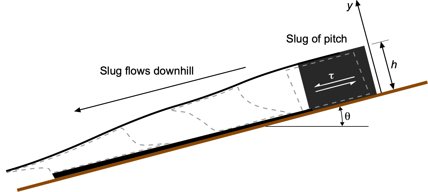
The local shear stress at a depth  below the free surface is
(136) 
and at the wall at , the shear stress becomes
(137) 
Newtonian Flow Assumption
Assume first a Newtonian fluid, where the shear strain rate is described by
(138) 
The velocity gradient in the slug is
(139) 
Integrating this equation gives the velocity profile, i.e.,
(140) 
and the corresponding maximum surface velocity is
(141) 
This is a parabolic velocity distribution, a well-known characteristic of viscous laminar flow.
It is also useful to express the velocity profile in non-dimensional form, i.e.,  . A non-dimensional vertical coordinate can be defined as
(142) 
and the corresponding dimensionless velocity is
(143) 
Substituting  into the expression for
  gives
gives
(144) 
Dividing by  gives the non-dimensional profile, i.e.,
(145) 
as shown in the figure below.
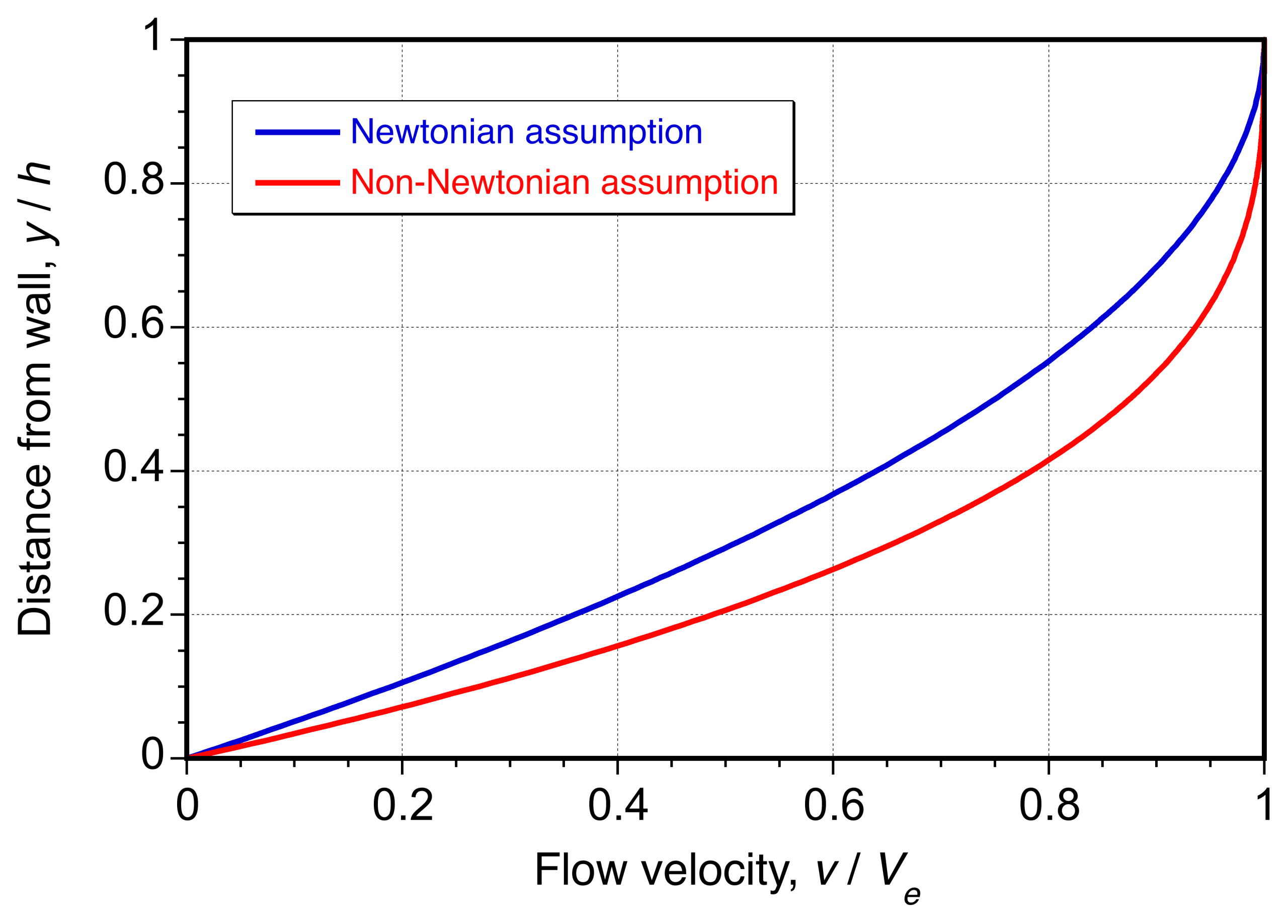
Non-Newtonian Flow Assumption
However, pitch generally follows a non-Newtonian law, where its effective viscosity depends on the shear rate. In this case, the power-law can be used as an approximation to the viscous behavior of pitch, i.e.,
(146) 
where  is a temperature-dependent coefficient and is the flow exponent. Inverting the relation gives the velocity gradient in terms of the local shear stress, i.e.,
(147) 
where  is the material consistency index. Integrating the velocity gradient gives the velocity profile, i.e.,
(148) 
At the free surface , the maximum velocity is
(149) 
In this case, the non-dimensional form of the velocity profile is
(150) 
as shown in the figure above for comparison. This solution reduces to the Newtonian case when , for which , and recovers the familiar parabolic velocity profile. While exact values of depend on temperature, composition, and aging, reported values for pitch and asphaltic materials consistently fall in the range  , depending on temperature, indicating a shear-thinning behavior. Regardless of the assumptions, the pitch will flow only very slowly under gravity and take a very long time to deform.
Kelvin’s pitch staircase vividly demonstrated the essential idea that whether a material behaves as a solid or a fluid depends not only on its composition, but also on the timescale of observation. Over the years, the original block of pitch, which initially appeared solid, slowly flowed down the wooden staircase, exemplifying a classic case of gravity-driven motion of a highly viscous fluid under conditions where inertial effects are negligible. In contrast, it is now known that glacier motion occurs through the slow deformation of ice, a crystalline solid, and Kelvin’s demonstration corrected the prevailing 19th-century belief that glaciers moved by rigid sliding.
Check Your Understanding #3 – Non-Newtonian flow of pitch down a slope
Consider a 1 cm thick slug of pitch on a  slope. The objective is to estimate the time required for the pitch to flow unswer gravity and reach a distance of 1 m down the slope. Assume a viscosity of
  Pa s and a density of
  kg/m, with = 0.85 for pitch. Consider both the Newtonian and non-Newtonian cases.
Show solution/hide solution.
For a Newtonian fluid, the surface velocity is given by
![\[ v_{\text{max}} = \frac{\varrho \, g \, h^2 \, \sin\theta}{2\mu} \]](https://eaglepubs.erau.edu/app/uploads/quicklatex/quicklatex.com-6737f721d2845ac8ed82babde565e51e_l3.svg "Rendered by QuickLaTeX.com")
Substituting the values gives
![\[ v_{\text{max}} = \frac{1000 \times 9.81 \times 0.01^2 \times \sin(10^\circ)}{2 \times 10^8} = 8.52 \times 10^{-10} \ \text{m/s} \]](https://eaglepubs.erau.edu/app/uploads/quicklatex/quicklatex.com-a0bf766851064473335a002b6ca69c99_l3.svg "Rendered by QuickLaTeX.com")
Therefore, the time required for the pitch to travel a distance of 1 m is
![\[ t = \frac{1}{v_{\text{max}}} = \frac{1}{8.52 \times 10^{-10}} = 1.174 \times 10^9 \ \text{s} \approx 37.2 \ \text{years} \]](https://eaglepubs.erau.edu/app/uploads/quicklatex/quicklatex.com-ca3b437125146f2bea809873ca260256_l3.svg "Rendered by QuickLaTeX.com")
For the non-Newtonian case, assume = 0.85 and = 10 Pa s
Pa s , where = 0.85. The surface velocity in this case is given by
![\[ v_{\text{max}} = \frac{n}{n + 1} \left( \frac{\varrho \, g \, \sin\theta}{K} \right)^{1/n} h^{\left(1 + \tfrac{1}{n}\right)} \]](https://eaglepubs.erau.edu/app/uploads/quicklatex/quicklatex.com-b16cf699c49921d8204dfc0b2c8b1e5c_l3.svg "Rendered by QuickLaTeX.com")
Substituting the given values gives
![\[ v_{\text{max}} = \frac{0.85}{1.85} \left( \frac{1,000 \times 9.81 \times \sin(10^\circ)}{10^8} \right)^{1/0.85} 0.01^{\left( 1 + \tfrac{1}{0.85}\right)} = 3.60 \times 10^{-12} \ \text{m/s} \]](https://eaglepubs.erau.edu/app/uploads/quicklatex/quicklatex.com-28817d76440ca8cd94df74cd44222df9_l3.svg "Rendered by QuickLaTeX.com")
and the corresponding travel time is
![\[ t = \frac{1}{v_{\text{max}}} = \frac{1}{3.60 \times 10^{-12}} = 2.78 \times 10^{11} \ \text{s} \approx 8,810 \ \text{years} \]](https://eaglepubs.erau.edu/app/uploads/quicklatex/quicklatex.com-032fe5f2cf93ff296aa471d1891d2884_l3.svg "Rendered by QuickLaTeX.com")
This dramatic difference arises not from a significant change in the nominal viscosity scale, but from the nonlinear dependence of the power-law model on both shear stress and film thickness, which strongly suppresses flow in low-shear conditions typical of shallow, slowly driven layers.
Microfluidics
Microfluidics is a field of fluid mechanics that is concerned with viscous-dominated fluid behavior at the microscale with characteristic dimensions of 1 to 1,000m (10 to 10
to 10 m). Unlike macroscale systems, where turbulence often plays a central role, microfluidic systems are characterized by smooth laminar, creeping (Stokes-like) flows with Reynolds numbers less than unity. Such flows often occur in combination with surface tension and capillary effects, as well as diffusion-driven flow mixing at the molecular level. As previously discussed in this chapter, creeping flows can be theoretically described by solutions to Stokes’ equation or its derived equations, providing a framework for understanding and designing effective microfluidic devices. Other related behaviors can be described semi-empirically in terms of well-established physical laws.
Applications
In aerodynamic research, microfluidic actuators may offer a promising approach toward achieving active flow control. For example, arrays of micro-flow actuators, supplied by microfluidic channels, could be pulsed or modulated to inject controlled momentum into the boundary layer. This approach may beneficially delay the onset of flow separation and delay stall, increasing lift and reducing drag. Likewise, microfluidic droplet generators can produce monodisperse tracer particles for particle image velocimetry (PIV). Unlike helium bubble generators, which release gas-filled bubbles into a flow, microfluidic droplet generators create liquid droplets with precise sub-micron size control. This improvement in seeding uniformity and measurement accuracy is especially beneficial in wind-tunnel testing for small-scale or transient flow features, where the particle time lag must be extremely short.
In the field of medicine and bioengineering, the high cost of many biological reagents provides a strong motivation to shrink down experiments to reduce the fluid volumes required. Fluid behavior at small scales also exhibits interesting and useful behaviors that can be exploited for precision control and fluid delivery. Experiments can be miniaturized to the point where flow channel sizes are of the order of micrometers and the working volumes are on the order of microlitres. In such systems, streams of fluid can be moved through tiny channels on a lab-on-a-chip device that is smaller than a postage stamp. These devices operate automatically and can complete processes much more rapidly than conventional laboratory methods.
A key function of microfluidics is distributing a sample to multiple points via capillary action, enabling different analytes to be quickly tested at each point. For example, as shown in the figure below, a chip-sized microfluidic device could distribute a tiny drop of blood to several testing regions. Each region can contain a different reagent or sensor, enabling rapid simultaneous detection of multiple biomarkers. Such devices already exist in commercial and research applications, offering the potential for reliable self-testing by patients at home, with minimal sample volume, fast turnaround time, and cost savings.
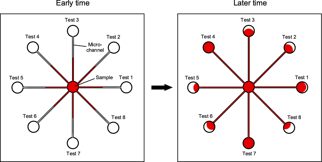
Theoretical Treatment
In microfluidic channels, the small dimensions result in very low Reynolds numbers, often much less than unity, where viscous forces govern the flow behavior. The use of this property is critical for the design of many microfluidic applications, where precise and predictable control of fluid movement is essential. Fluid motion in microchannels can be driven by a variety of mechanisms, including pressure gradients (producing Poiseuille-type flows), capillary action in pump-free designs, electro-osmotic effects under applied electric fields, and even centrifugal or acoustic forces in specialized devices. However, a pressure-driven flow is the most common mechanism in simple microchannel networks.
Pressure-Driven Flow
For a Newtonian fluid under steady, fully developed, laminar flow in a circular channel, the Hagen-Poiseuille relation is applicable, i.e.,
(151) 
where is the volumetric flow rate,  is the pressure drop, is the channel radius, is the dynamic viscosity, and is the channel length. The dependence of on
  highlights the sensitivity of microchannel flows to the geometric dimensions. For example, a reduction of just 10% in channel radius results in approximately a 35% decrease in flow rate for the same pressure drop. In practical microfluidic devices, these factors make fabrication accuracy and dimensional stability critical for consistent performance.
Many microfluidic channels are rectangular rather than circular, but it is incorrect to replace with an equivalent hydraulic radius in the Hagen-Poiseuille formula. Instead, the rectangular section Poiseuille relation must be used, i.e.,
(152) 
where the aspect-ratio correction  accounts for side-wall friction losses using Eq. 38. For example,
  for a square duct and
  .
.
However, in microfluidics, it is still conventional to define dimensionless groups that use a length scale as a reference, such as the Reynolds number, using the hydraulic diameter, i.e.,
(153) 
where is the cross-sectional area and  the wetted perimeter of the channel.
Diffusion & Mixing
Unlike macroscale systems, where turbulence facilitates mixing, microfluidic systems operate under laminar flow, so molecular diffusion becomes the primary mechanism of mixing. Fick’s first law of diffusion describes the diffusion flux,  , as
, as
(154) 
where is the diffusion coefficient and  is the concentration gradient; see the chapter on fluid properties. The characteristic time for a molecule to diffuse across a distance is given by
(155) 
In microchannels, the small values of reduce the values of  significantly, allowing relatively fast molecular transport even without turbulence. However, in many practical applications, this natural diffusion rate may still be insufficient. In such cases, the microchannel geometry can be engineered to enhance mixing using serpentine channels, which lengthen the flow path and allow natural diffusion to continue, as shown in the figure below.
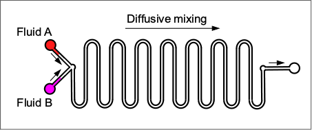
The efficiency or natural rapidity of molecular mixing in microfluidic systems is often quantified using the Péclet number ( ), which compares the relative importance of advection (bulk fluid motion) to diffusion (molecular transport), i.e.,
(156) 
where is the characteristic flow velocity, is a characteristic length scale, and is the molecular diffusion coefficient. Physically, the Péclet number can be interpreted as the ratio of two time scales, the time for a fluid particle to be advected by the flow a distance ( ) and the time for a molecule to diffuse the same distance (
 ). Therefore,
(157) 
When the value of  , diffusion is relatively fast compared to advection, and mixing occurs rapidly without the need for complex channel designs. When
  , then advection dominates and diffusion is relatively slow, so mixing is poor unless additional geometric features such as serpentines or other flow manipulations are introduced. In microfluidic systems, the Reynolds number is typically very low (), meaning that flows remain laminar throughout; however, the values of can vary widely depending on mixing performance and for determining whether passive diffusion or active mixing strategies will be required in device design.
Capillary Effects
Capillary forces play a significant role in microfluidics, particularly in systems that use narrow channels without external pumps. The driving mechanism is the pressure difference across the curved liquid-air interface (the meniscus), given by the Young-Laplace relation, i.e.,
(158) 
where is the liquid-air surface tension, is the contact angle with the channel wall, and is the channel radius; see the chapter on fluid properties. This pressure difference draws liquid into the channel until opposing forces balance it.
In the well-known case of a vertically oriented tube, gravity provides the opposing force. The liquid rises until hydrostatic pressure balances the capillary suction, yielding the classical capillary rise height, i.e.,
(159) 
where is the fluid density and the gravitational acceleration. In a horizontal tube, gravity does not oppose the motion, so the liquid advances along the channel until viscous drag balances the capillary pressure. The penetration length  is then governed by the Washburn equation, i.e.,
(160) 
where is the viscosity of the liquid. This equation shows that the liquid front advances with the square root of time. By carefully controlling the channel dimensions, surface chemistry, and wetting properties, capillary forces can be harnessed in both vertical and horizontal geometries to drive spontaneous fluid transport in microfluidic devices without external pumping.
The balance between viscous and capillary forces is commonly expressed by the capillary number, i.e.,
(161) 
where is the fluid viscosity, is a characteristic velocity of the advancing liquid, and is the surface tension. Small values of  indicate surface-tension-dominated motion, as in spontaneous capillary rise or imbibition, while large values of correspond to viscous-dominated regimes where capillary effects become negligible.
Electric-Fields
Electric fields can be used to manipulate fluids in microfluidic systems. Electro-osmotic flow (EOF) is a key mechanism for moving fluids in channels with charged walls. When an electric field is applied, the interaction between the field and the electric double layer at the channel surface generates fluid motion. The velocity of electro-osmotic flow,  , is given by
(162) 
where  is the permittivity of the fluid,
  is the zeta potential at the channel wall,
  is the electric field strength, and is the fluid’s dynamic viscosity. An electric field for electro-osmotic flow is created by placing electrodes in the inlet and outlet reservoirs of a microchannel and applying a voltage across them, producing
![\[ E \approx \frac{V}{L} \]](https://eaglepubs.erau.edu/app/uploads/quicklatex/quicklatex.com-23c66ee82c8286ab8b923b7c21fdffb0_l3.svg "Rendered by QuickLaTeX.com")
where is the applied voltage potential (do not confuse with velocity) and is the channel length. This field acts on the counterions in the electric double layer, dragging the bulk fluid and generating an EOF. An EOF is particularly advantageous for precise fluid control because it eliminates the need for mechanical pumps and enables the manipulation of tiny fluid volumes with high control.
Pumps
Microfluidic pumps drive fluid through microscale channels using various mechanisms. The most common approaches are pressure-driven pumps (syringes or regulators), electrokinetic pumps (electric fields inducing electro-osmotic flow), and micromechanical pumps (valves or membranes actuated by piezo, pneumatic, or thermal means). Simpler devices may also rely on passive methods such as capillary action or centrifugal forces for fluid transport without external equipment.
Droplets
In droplet-based microfluidics, droplet formation and manipulation are governed by surface tension, as described by the Young-Laplace equation. This equation relates the pressure difference across a curved liquid interface to the surface tension ) and the radii of curvature  and
and  , i.e.,
(163) 
This principle is essential for understanding how droplets form, merge, and break apart in microfluidic systems. By controlling the channel geometry and fluid flow rates, researchers can precisely manipulate droplet size and behavior, which is helpful for various applications.
A closely related phenomenon is bubble formation, which occurs when a gas thread enters a liquid-filled microchannel and pinches off into discrete bubbles. The same Laplace pressure governs the stability of the gas-liquid interface, resisting deformation and controlling bubble detachment. The capillary number quantifies the balance between viscous and capillary forces. As shown in the schematic below, at low values of , surface tension dominates and bubbles form in the squeezing regime, with bubble size mainly determined by channel geometry. At intermediate values, viscous shear promotes detachment in the dripping regime, and bubble size decreases with increasing liquid flow rate. At high , the gas forms a continuous jet that breaks into bubbles downstream in the jetting regime.
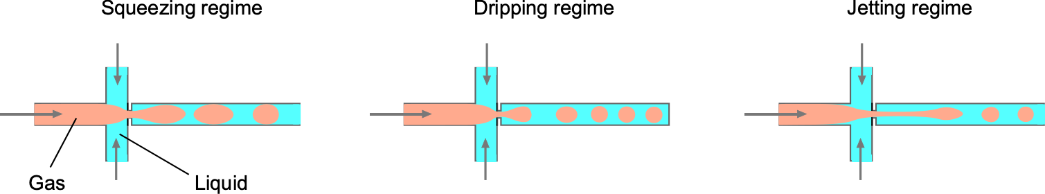
At low , the bubble length  often follows a simple scaling relation, i.e.,
(164) 
where  is the channel width,
  and
and  are the volumetric flow rates of the gas and liquid phases, respectively, and
  is an empirical constant of order unity. These relations show how channel design and flow conditions can be tuned to control droplet or bubble size, frequency, and stability.
Microfluidic Pressure Sensor
By applying the foregoing principles, engineers can design a wide range of devices that leverage the unique properties of microscale fluid dynamics to achieve precise control over fluid motion and mixing. Understanding the fundamental mathematical foundations of microfluidics is essential for advancing the field and unlocking its full potential across a multitude of applications. For example, one of the challenges aerospace engineers face is measuring various types of pressures, which are crucial in many contexts, including airspeed and altimetry. Conventional pressure transducers are based on resistive changes in strain on a piezo element, which is suitable for many applications. But microfluidics has enabled the design of other types of pressure sensors, including the one shown in the figure below.
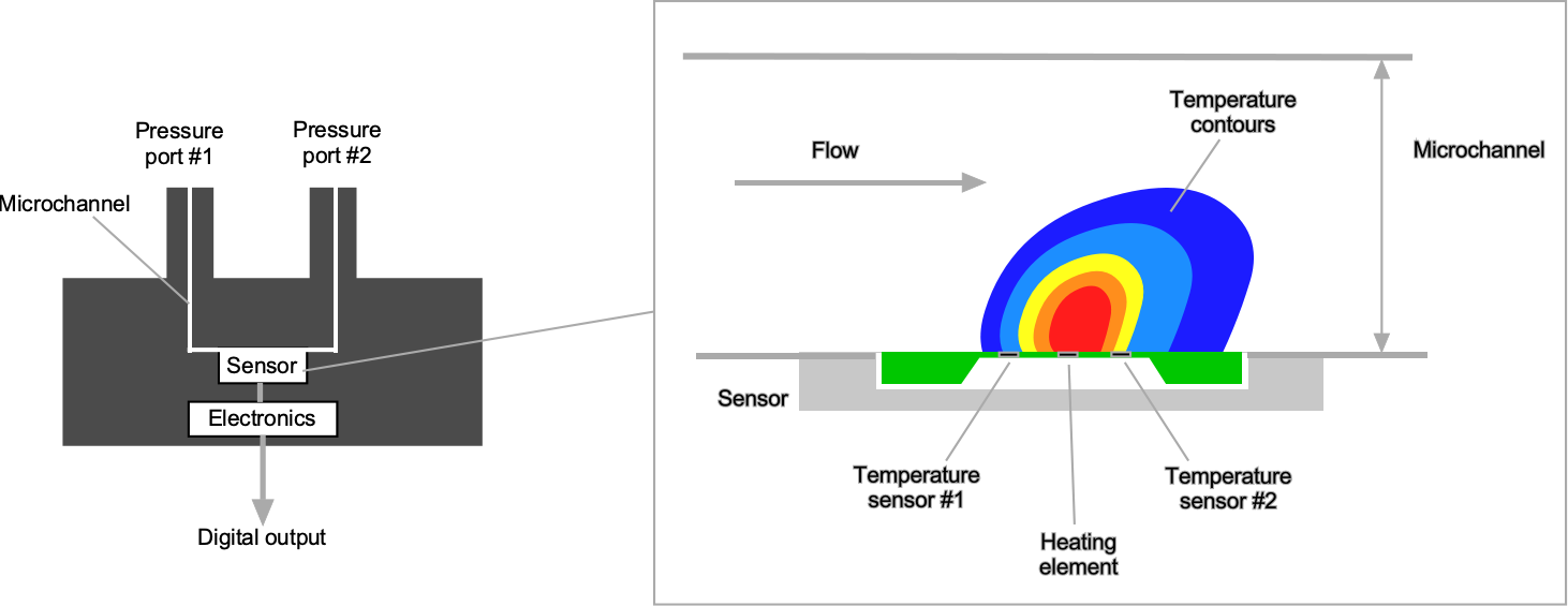
This sensor consists of a narrow internal microchannel connecting two external pressure ports. A tiny heater is located at the center of the channel, flanked by two temperature sensors on the upstream and downstream sides. When a pressure difference is applied across the ports, it drives a tiny amount of bleed flow through the microchannel. This flow convects heat from the heater downstream, creating a temperature differential between the two sensors. The magnitude and direction of this temperature difference are directly proportional to the mass flow rate through the channel, which can then be calibrated to measure the differential pressure across the ports. This thermal sensing approach enables extremely high sensitivity and the measurement of low-pressure differences.
Check Your Understanding #4 – Flow parameters in a microchannel
Water at  C, with viscosity = 1.0
 10 Pa s, density = 1.0 10
 kg/m, and surface tension = 0.072 N/m, flows through a microchannel of width = 200 m, height = 50 m, and length = 2 cm. At the entrance, a Y-junction merges two streams, with one containing a solute while the other is water. The solute has diffusivity = 1.0 10
 m
m /s. The volumetric flow rate is = 2 L/min. Determine the pressure drop along the channel length , the mean flow velocity in the channel, the numerical values of the relevant similarity parameters, and the downstream diffusive mixing lengths.
Show solution/hide solution.
To determine the pressure drop, the Poiseuille equation for a rectangular channel can be used, i.e.,
![\[ Q = \frac{\alpha (\lambda) \, w \, h^3}{12 \mu}\left( \frac{\Delta p}{L} \right), \quad \text{where} \quad \alpha( \lambda ) \approx 1 - 0.630 \left( \dfrac{h}{w} \right) + 0.053 \left(\dfrac{h}{w}\right)^5 \]](https://eaglepubs.erau.edu/app/uploads/quicklatex/quicklatex.com-65cb971ddb93786f68cb627930900de4_l3.svg "Rendered by QuickLaTeX.com")
Here  = 0.25 giving
  0.843. The volumetric flow rate is given, so converting to base units gives
![\[ Q = \frac{2\times 10^{-9}}{60} = 3.33\times 10^{-11}\ \text{m}^{3}/\text{s} \]](https://eaglepubs.erau.edu/app/uploads/quicklatex/quicklatex.com-d225e7785f3d74cafa51d53392b7034e_l3.svg "Rendered by QuickLaTeX.com")
Substituting the other numerical values yields
![\[ \Delta p=\frac{12\,\mu\,L\, Q}{\alpha\,w\,h^{3}} =\frac{12(1.0\times10^{-3})(0.020)\, (3.33\times10^{-11})}{0.843\,(200\times10^{-6})\,(50\times10^{-6})^{3}} = 3.8\times10^{2}\ \text{Pa} \]](https://eaglepubs.erau.edu/app/uploads/quicklatex/quicklatex.com-cddcf726a88a359e725800b15fa3ef26_l3.svg "Rendered by QuickLaTeX.com")
The cross-sectional area is  = 1.0 10
 m
m , so the average flow velocity is
![\[ U =\frac{Q}{A}=\frac{3.33\times10^{-11}}{1.0\times10^{-8}} = 3.33\times10^{-3}\ \text{m/s} \]](https://eaglepubs.erau.edu/app/uploads/quicklatex/quicklatex.com-44039ec11fca9979a7aa9bdb79e0a13d_l3.svg "Rendered by QuickLaTeX.com")
Using the hydraulic diameter  = 80 m (do not confuse
  with the diffusivity coefficient, ), the similarity parameters become
(165) 
For the Péclet number referenced to the channel height ( = 50 m = 5.0 10 m), then
(166) 
If needed, the diameter-based Péclet number is  .
.
For the capillary number, then
(167) 
The diffusion time across a distance  is
is  , giving a streamwise mixing length
  (here = 3.33 10 m s
 and = 1.0 10 m/s. Across half the height
  = 25m, so
![\[ t_{d,h}=\frac{(25\times10^{-6})^{2}}{1.0\times10^{-9}}= 0.625\ \text{s},\qquad L_{\text{mix},h} = U\,t_{d,h}=(3.33\times10^{-3})(0.625) = 2.1\ \text{mm}<L \]](https://eaglepubs.erau.edu/app/uploads/quicklatex/quicklatex.com-cbc0fa98631b21d5618a56b46241e12e_l3.svg "Rendered by QuickLaTeX.com")
with  , so the solute becomes nearly uniform vertically within the channel. Across half the width
  , then
![\[ t_{d,w} = \frac{(100\times10^{-6})^{2}}{1.0\times10^{-9}} = 10\ \text{s},\qquad L_{\text{mix},w} = U\,t_{d,w}=(3.33\times10^{-3})(10) = 3.3\ \text{cm}>L \]](https://eaglepubs.erau.edu/app/uploads/quicklatex/quicklatex.com-57b54bc17e815a1a315fe44c5882e730_l3.svg "Rendered by QuickLaTeX.com")
so lateral mixing is incomplete by the outlet. Therefore, the two inlet streams remain stratified in the lateral direction at the outlet unless a serpentine or active mixing is introduced. In summary, the flow is in the creeping-flow/low- regime ( ) with a slight pressure drop of
  380 Pa. Vertical mixing occurs within the channel, but lateral mixing is incomplete over its length.
Summary & Closure
Viscous-dominated (Stokes) flow arises when the Reynolds number is very small, such that inertia can be neglected and the Navier-Stokes equations reduce to the linear Stokes form. This regime, often termed creeping flow, is characterized by smooth, reversible motion and the ability to use superposition to construct solutions. Canonical examples include flow past a sphere, which leads to Stokes’ drag law, and confined flows such as planar Couette and Poiseuille flow. For slightly higher Reynolds numbers, the Oseen approximation extends the analysis by incorporating weak inertial effects.
The principles of Stokes flow provide the basis for understanding particle settling and sedimentation processes, lubrication theory, and viscous instabilities such as Taylor-Couette flow. They also extend to the behavior of non-Newtonian fluids, where viscosity depends on shear rate, broadening the range of physical applications. In modern practice, the governing equations underpin microfluidic technologies that exploit precise viscous control for diagnostics and research. Taken together, these ideas highlight the enduring importance of Stokes flow as both a theoretical framework and a practical tool. From classical drag laws to contemporary microfluidics, viscous-dominated flows illustrate how the simplest limit of fluid mechanics continues to shape innovations in aerospace, mechanical engineering, and the broader scientific community.
5-Question Self-Assessment Quickquiz
For Further Thought or Discussion
- Explain the significance of the Reynolds number in distinguishing flows around spheres.
- How do the characteristics of viscous-dominated flows differ from inertial-dominated flows?
- What are some real-world applications where viscous-dominated flows are found?
- How do the Stokes equations simplify the analysis of flows at low Reynolds numbers?
- Why is time reversibility a characteristic of viscous-dominated flows?
- How might non-Newtonian fluids behave in viscous-dominated flow regimes?
- How does energy dissipation differ in viscous-dominated versus inertial-dominated flows?
- What might happen if a small ball bearing is dropped into a container of ketchup?
Other Useful Online Resources
To learn more about viscous-dominated flows, take a look at some of these online resources:
- Graduate Fluid Mechanics Lesson Series – Stokes Flow Over a Sphere.
- Graduate Fluid Mechanics Lesson Series – Observations: Stokes Flow Over a Sphere
- A demonstration of the reversibility of Taylor-Couette flow.
- Low Reynolds number flows: Lecture on the derivation of the Stokes equation.
- Nothing in fluid mechanics is ever easy. ↵
- See: Happel, J., and Brenner, H. (1983). "Low Reynolds Number Hydrodynamics: With Special Applications to Particulate Media,'' Martinus Nijhoff Publishers, Leiden. ↵
- Irrotational flow is a feature only of ideal (non-viscous) fluid models. ↵
- Henry Hele-Shaw (1854–1941) introduced the Hele-Shaw cell in the late 19th century as a practical tool to study fluid motion in thin layers. Porous media were difficult to study directly, but the cell provided a controlled experimental setting in which flow patterns could be observed and photographed. He realized that the equations for depth-averaged viscous flow between two closely spaced plates reduce to the same form as Darcy’s law for porous media flow. ↵
- While ellipses have a strict geometric definition, ovals encompass a broader range of mathematically and visually rounded shapes. ↵
