Advanced computational methods continue to be developed to analyze challenging problems in aerospace engineering. Such methods include aerodynamics, structural analysis, and coupling disciplines such as aeroelasticity and flight dynamics. In particular, computational fluid dynamics, commonly referred to as “CFD,” and the finite element method, or “FEM,” have been revolutionary computational tools for predicting aerodynamics and structural loads, respectively. The intention of this chapter is not to review the details of such techniques and their associated numerical algorithms in themselves, but to provide an introduction and general overview of the foundational principles and how they are applied, along with a summary of their capabilities and some of their limitations. Nor is it meant to be an all-encompassing treatment, far from it.
Traditionally, the aircraft industry has relied on quicker and more economical computational methods for designing aircraft and predicting their flight performance, achieving success in doing so. One does not need CFD or the FEM to design and build a flight vehicle that works as intended; history speaks for itself. However, both tools can significantly help refine the aircraft design to extract its maximum performance at the lowest cost, with the added benefit of improving safety and reliability. Understanding why something works (or doesn’t) is crucial to achieving commercial success and driving continued technological advancement. Wind tunnel testing has always been a critical part of the flight vehicle design process and will continue to be essential for measurements used in CFD validation. Advances in computer technology, such as code execution speed, memory, data storage access speed, and the availability of inexpensive mass data storage systems, continue to encourage the development of more ambitious numerical methods for use during the design process.
Significant new fundamental research in modeling and algorithmic development has been conducted over the last two decades. Aerodynamics and structural problems, once relegated to the fastest available supercomputers at national centers, can now be solved using local computational resources. For example, most universities today have powerful computer clusters, allowing for research into new computational methods for use in various technical fields. As shown in the image below, the ability to predict flows about complete aircraft can open up opportunities in new design directions, such as the reconsideration of supersonic transports (SSTs). It has also inspired broader innovations in flight vehicle designs, allowing concepts outside the domain of conventional wisdom to be investigated with confidence. Thinking “out of the box” can now be quantified for the right reasons!
An advanced CFD solution around a proposed SST aircraft can be used to explore configurational changes at the design stage. (NASA public domain image.)
Continued advances in computer capabilities, which continue to accelerate,[1] has also played a large part in motivating and accelerating the development of more integrated computational techniques, encompassing several traditionally separate engineering disciplines. For example, the governing equations and solution methods used in one field are rarely the same as those used in another; therefore, some form of method coupling is required. Increasingly tighter mathematical, algorithmic, and numerical coupling has enabled, for example, the simultaneous solution of the coupling between aerodynamics and structural dynamics. If fully realized, this integration strategy will eventually enable the prediction of an entire flight vehicle’s behavior in arbitrary flight conditions, allowing for more capable and efficient vehicle designs. However, significant integration problems and more advanced numerical techniques are still required to further develop this technology, with the ultimate goal of predicting the vehicle’s characteristics before its first flight.
Learning Objectives
Understand the foundational elements of modern computational aerodynamic methods, starting from the governing Navier-Stokes equations.
Appreciate the hierarchy of such aerodynamic methods in terms of their relative predictive advantages and disadvantages.
Know about surface singularity methods and their capabilities and limitations for aerodynamic prediction.
Understand why boundary layers have a significant impact on aerodynamic behavior and why their modeling is crucial.
Appreciate the fundamentals of the structural finite element method and its uses.
Discover the field of aeroelasticity and its importance in the design of flight vehicles.
Aerodynamics
Over the past three decades, significant advances have been made in understanding challenging problems in aerodynamics through the use of computational fluid dynamics (CFD). Numerical methods, such as finite-difference methods (FDM) or finite-volume methods (FVM), are applied to the governing flow equations (e.g., the Navier-Stokes equations) to model the flow field around an aircraft. The choice of governing equations to use affects the level of physics that can be approximated by the CFD scheme, as well as the computational effort and time required to solve it. Not all numerical methods are created equally, and the choice of method has a significant impact on the accuracy, stability, and cost of the solution. The definition of “cost” comes down to how much time[2] and effort go into obtaining a solution, and most CFD methods are considered costly by any design standard.
Developing comprehensive CFD methods is typically considered the ultimate in aerodynamic modeling. So far, a wide range of numerical techniques has been used to solve a hierarchy of equations governing the flow, ranging from irrotational and inviscid potential flow approximations to the Euler and Navier-Stokes equations. The latter set of equations can resolve the effects of compressibility, thermodynamics, and turbulence. Each level in the hierarchy of governing equations increases physical modeling capability but also requires more computational effort and cost for the solution.
A key issue in using these numerical methods is the definition and creation of appropriate computational grids over which to solve the governing equations, requiring considerable skill and effort. Other problems include the difficulties in modeling flow turbulence, for which no single method exists. Furthermore, CFD methods must be validated against measurements to realize the high predictive confidence levels needed for aircraft design work. Commercially available tools, such as ANSYS Meshing and Pointwise, can aid in grid generation, while CFD solvers like ANSYS Fluent and OpenFOAM can perform the actual CFD simulations. However, there are also many other options for grid generation and CFD solvers.
History
The earliest numerical solutions to viscous flow problems about bodies go back almost a century. Alexander Thom, a Carnegie Fellow at the University of Glasgow, published a paper in the Proceedings of the Royal Society in 1933 titled: “The Flow Past Circular Cylinders at Low Speeds.”[3] In this work, the viscous flow was solved over a numerically defined grid by “arithmetical” means. Back then, there were no digital computers, so calculations were performed “by hand,” i.e., using a pencil, paper, a slide rule, and perhaps a mechanical calculator. Thom remarked in his paper that the “whole process is long,” but his computed results compared favorably with flow experiments.
The advent of digital computers in the 1950s provided the computational power to begin to tackle numerical solutions to the governing equations of fluid dynamics. Early work by pioneers such as John von Neumann and his collaborators laid the groundwork for numerical methods to solve partial differential equations. Von Neumann is often referred to as the “Father of Modern Computer Architectures.” During the 1960s, CFD began to evolve more rapidly in parallel with advances in computer technologies. Developing algorithms based on finite difference, finite element, and finite volume methods enabled more accurate and efficient solutions of the various forms of the governing equations of fluid dynamics. Finite-difference techniques were already well established by then, starting from Brook Taylor[4]in the early 1700s, with other contributions by Leonhard Euler and Carl Runge. There was also much new work in numerical methods, and the accuracy and stability of such schemes were increasingly crucial for solving aerospace problems.
The publication of many technical papers and essential textbooks during the 1960s helped to disseminate these numerical methods and apply them to fluid flow problems. Textbooks by Brian Spalding[5] and Suhas V. Patankar[6] were used to teach CFD to students as part of courses in fluids. NASA and other aerospace laboratories worldwide have played a crucial role in advancing CFD for practical applications in aerospace engineering. In 1987, NASA established the Advanced Supercomputing Division (ASD) at NASA Ames. Additionally, the U.S. Army Aeronautical Research Laboratory played a crucial role in advancing the CFD field. The first commercial CFD software packages emerged during this period, making the technology accessible to a broader range of engineers and researchers.
The 1980s and 1990s saw substantial improvements in numerical techniques, computational power, digital memory, and storage devices. Desktop computers were still somewhat limited in their capabilities, and most serious computational work was done on “mainframe” computers. Remotely accessible supercomputers, such as the CRAY, became available, and desktop computers also became increasingly capable, allowing for more complex CFD simulations at a local level. Advances in turbulence models, grid generation techniques, and numerical methods continued to contribute to more accurate and robust CFD solutions. During this period, CFD also started to find applications beyond the aerospace field, including automotive, chemical, and civil engineering.
CFD has continued to advance from the early 2000s to the present, with the development of more sophisticated algorithms, increased computational power, and the emergence of parallel computing. High-performance computing (HPC) and graphics processing units (GPUs) have become increasingly commonplace, enabling the simulation of more complex and larger-scale aerospace problems. Additionally, CFD has benefited from advancements in data visualization techniques, making it easier for engineers to interpret and analyze large quantities of data and understand complex flows. Today, CFD is an essential tool in engineering analysis, with applications ranging from designing flight vehicles to weather prediction, biomedical engineering, and environmental studies. The continuous development of software, increased accessibility of computational resources, and ongoing research mean that CFD will remain at the forefront of future scientific and engineering innovation.
Navier-Stokes Equations
Most aerodynamic problems with flight vehicles involve viscous effects and turbulence. These effects are significant in the turbulent boundary layers found on the wings and airframe, as well as in a host of component interaction phenomena, such as wing/fuselage interference and powerplant/wing interference. Modeling flow separation is also essential, as the onset can set boundaries for an aircraft’s operational flight envelope. The Navier-Stokes equations are the fundamental equations that govern fluid dynamic behavior. They encompass the principles of conserving mass, momentum, and energy, as well as the interchange of these within a fluid.
The Navier-Stokes equations are a set of coupled, highly nonlinear partial differential equations. This means they can only be solved by making simplifying assumptions, which in some cases may be rather sweeping. The most common practical simplification is to avoid treating turbulence and the associated viscous shearing effects by assuming a laminar flow. While this approach simplifies the Navier-Stokes equations, it is worth noting that flows will still be turbulent even at the lowest Reynolds numbers encountered on aircraft.
Tensor Form
The tensor form is often used to express the Navier-Stokes equations. The conservation of mass (continuity equation) is given by
(1)
and in tensor form by
(2)
where is the flow density and , , is the velocity vector. For an incompressible flow, where = 0, then
(3)
Conservation of momentum (momentum equation) gives
(4)
and in tensor form by
(5)
where is the pressure, is the stress tensor, and is a body force per unit mass, e.g., acceleration under gravity.
Modeling Viscous Effects
The Navier-Stokes equations are general and apply to all flows, including flows with turbulence. The flow about an aircraft, at least at lower Mach numbers, can be readily approximated as an isotropic Newtonian fluid, for which the relationship between stress and strain in the Navier-Stokes equations is given by
(6)
where is the Kronecker delta function, i.e., for , and otherwise, and is the coefficient of dynamic viscosity. The parameter is called the second coefficient of viscosity or bulk viscosity, usually given as , which is referred to as Stokes’s hypothesis.[7] The bulk viscosity, which can be measured, as can , is essential in describing the compression and energy dissipation in fluids, both gases and liquids, such as in sound wave propagation, shock waves, and other phenomena.
Notice from either Eq. 12, for an incompressible flow where , then the term involving vanishes, so the stress tensor depends only on the dynamic viscosity, . For a compressible flow, however, the term represents the rate at which the fluid’s density changes under compression or expansion. Therefore, the term in the stress tensor accounts for the viscous stresses arising from these volume changes.
Rounding out the conservation laws is the conservation of energy (energy equation), which can be expressed as
(7)
and in tensor notation
(8)
where is the internal energy per unit mass, is temperature, is the bulk thermal conductivity, and is the external heat per unit mass. Finally, the ideal gas equation (equation of state) can be used to relate the thermodynamic quantities, i.e.,
(9)
where is the gas constant. Recall that the equation of state is one of the few truly “handy” equations in aerodynamics.
Conservation Form
For practical use, the Navier-Stokes equations are usually rewritten more compactly in the so-called conservation form, compared to the tensor differential form given previously, i.e.,
(10)
where is the conserved variable vector and , , and are the flux vectors. The flux vectors express the rate at which mass, momentum, and energy are transported at any flow point. This latter equation is often expanded into a form with the viscous terms on the right-hand side to give
(11)
where , , and are the fluxes resulting from the viscosity of the flow.
This form of the governing equations allows a mathematical reduction to a simpler form called the thin-layer Navier-Stokes equations, where the viscous derivatives with respect to the and directions are neglected to give
(12)
for a suitably defined viscous flux, , that accounts for the neglected derivatives.
The thin-layer Navier-Stokes equations are particularly useful in scenarios where the flow can be approximated as two-dimensional or quasi-two-dimensional, simplifying computational efforts and modeling complexities. Engineers often apply these simplified equations in boundary layer analyses, fluid film lubrication, and other situations where the flow dynamics are primarily in the and directions.
Reynolds-Averaged Navier-Stokes (RANS) Form
The Reynolds-Averaged Navier-Stokes (RANS) equations are a form of the Navier-Stokes equations to describe the flow of incompressible fluids. These equations are particularly useful in the study of turbulent flows. The key idea behind the RANS equations is to decompose the instantaneous quantities (such as velocity and pressure) into their mean (time-averaged) and fluctuating components.
The Navier-Stokes equations for an incompressible fluid can be written as
(13)
and
(14)
where represents the external body forces per unit mass.
In the Reynolds decomposition, the instantaneous velocity and pressure are decomposed into mean and fluctuating components, e.g., for the component of velocity, then
(15)
and for the static pressure
(16)
Here, and are the mean (time-averaged) components, while and are the fluctuating components, as illustrated in the figure below.
The classic Reynolds decomposition splits the turbulent flow properties into a statistical mean (average) and a statistically fluctuating part.
When the Navier-Stokes equations are averaged over time, the nonlinear term introduces additional terms that account for the Reynolds stresses, which are the stresses created by the turbulent fluctuations. The averaged form of the continuity and momentum equations then becomes
(17)
and
(18)
The term represents the divergence of the Reynolds stress tensor, which arises from the turbulent fluctuations. This term is often modeled using various turbulence models, which will be discussed later, because it cannot be directly calculated from the mean flow variables.
The RANS equations give a CFD method that strikes a balance between computational cost and accuracy, making them a popular choice for many practical fluid dynamics problems. RANS methods are widely used in engineering and scientific applications to predict and analyze turbulent flows in various contexts, including aircraft and automobile design, ship hull design, water flow in pipes, weather forecasting, and environmental engineering, such as pollutant dispersion. Several CFD software packages are available to solve the RANS equations, including ANSYS Fluent, OpenFOAM, COMSOL Multiphysics, and STAR-CCM+.
Gridding of the Computational Domain
Numerous algorithmic developments have occurred in the numerical solution of the Navier-Stokes equations. A fundamental issue in any flow problem involving a body is generating a grid structure that represents the body’s geometry, on which to solve the governing equations. This means that the size of the computational domain should be as small as possible for economic reasons, yet large enough to avoid nonphysical issues within the domain, which can result in extensive computer memory requirements.
Several types of grid systems are appropriate for analyzing flow problems; a summary is shown in the figure below. Grids are typically categorized by their geometric shape, such as O-grids, C-grids, and H-type grids. The O-grids and C-grids are often used to analyze flows around wings, as they can conform to the curved airfoil shape of the surface, which are called body-fitted grids, as shown in the figure below. H-type grids are also used; they allow a compromise between the advantages of a Cartesian grid geometry and the ability to refine the grid near a surface to resolve the boundary layer. Nodes are the intersection points on the grid, and these nodes form a cell. The numerical solution to the flow properties is then based on finite-difference or finite-volume solutions applied over the nodes and cells.
Types of elementary grids used as a basis for solving problems in computational fluid dynamics.
As shown in the figure below, creating a CFD grid for a wing or other lifting surface involves defining its geometry accurately and refining the grid to capture the flow details. It must include fine surface meshes to resolve boundary layer flows, denser grids near the wing tip to accurately capture the formation and roll-up of the wing tip vortices, and smooth cell transitions to prevent any numerical discretization issues. Adaptive Mesh Refinement (AMR) may better capture transient (time-dependent) phenomena. This approach ensures an accurate representation of aerodynamic characteristics.
Creating CFD grids for a wing and wing tip requires considerable care to compute the flow correctly.
Overset or chimera grid systems are locally refined grids superimposed upon a primary or background grid, as shown in the figure below, which is like adding a grid patch where and when needed. These overlapping grids help resolve local flow phenomena without gridding the entire flow domain at high resolution, thereby saving computational effort. They can also be used to overcome specific difficulties in dealing with a domain that is most easily meshed using separate grids that move relative to each other, such as propellers and rotors relative to an airframe.
Chimera grids, which are overlapping “patch” grids, allow for local grids without requiring grid refinement of the entire CFD domain. (NASA image.)
With chimera grids, interpolation methods are required to transfer flow property information between the grids. The accuracy of these procedures needs to be carefully examined to ensure the overall accuracy of the numerical solution is maintained. Such grids can also be very labor-intensive to create. Unstructured grids, composed of irregularly distributed tetrahedral elements, as illustrated in the figure below, are being increasingly used. They have the advantage that semi-automatic mesh generation software can create this grid type around complex surface geometries. Such grids also have the advantage of reaching a more optimal number of grid points, thereby speeding up the numerical solution and reducing cost.
An unstructured “irregular” grid is composed of random tetrahedral elements.
Turbulence Modeling
Modeling turbulence in most flow problems requires introducing empirical “closure” models, of which many types have been developed. Indeed, resolving all turbulence scales requires extremely fine grids with precise numerical discretization, demanding large amounts of memory and the fastest computers. Calculating turbulence remains complex even for the most straightforward flows and is impractical for flows around complete aircraft.
The viscous stresses can be expressed in the form
(19)
where . This latter formulation implies that
(20)
Here, is known as the eddy viscosity, representing an effective viscosity resulting from the effects of turbulence. Therefore, turbulence models that aim to simulate variations in eddy viscosity in the flow are called eddy viscosity models. In these models, higher levels of turbulent stresses are simulated by augmenting the effects of molecular viscosity alone with a turbulent viscosity coefficient, i.e.,
(21)
This preceding result assumes that the turbulent stress tensor is proportional to the mean strain rate tensor multiplied by a constant, known as the Boussinesq hypothesis. It also assumes that the exchange of turbulent energy in the cascading process of eddies is analogous to the effects of molecular viscosity, as illustrated in the figure below. Many experiments and observations of turbulent flows support this behavior. Therefore, the Boussinesq hypothesis implies that turbulent flow can be modeled as an effective total viscosity that varies with local flow conditions.
The concept of an “eddy” viscosity is used to augment the laminar molecular viscosity from the effects of mixing caused by turbulence.
Therefore, with the addition of turbulence in the form of an eddy viscosity, the Navier-Stokes equations can be modified into the form
(22)
Eddy viscosity models belong to a class of so-called “turbulence models” or “turbulence closure models,” which provide a mathematical basis for solving the mean flow field and the turbulent flow quantities. Many different turbulent flow models are available, particularly for use in computational fluid dynamics (CFD), and selecting the most suitable turbulence model requires careful consideration of the specific problem. The best way to represent turbulent viscosity and decide on the most suitable turbulence model depends on several factors, including the specific flow application, the desired level of numerical accuracy, and the available computational resources.
Deciding on the types of turbulence models that can be expected to give good predictive capability depends on understanding the length and time scales of the specific flow problem at hand. It should be appreciated that turbulent flows exhibit a wide range of spatial scales, each of which plays a vital role in the overall behavior of the flow. The spatial scales of turbulence can be broadly classified into three categories: large, intermediate, and small eddies, as illustrated in the figure below. Therefore, there is no “one size fits all” turbulence model. The different scales of turbulence interact in a complex manner, and a wide range of phenomena, such as vorticity, turbulence intensity, and Reynolds stresses, characterize their behavior. Modeling these scales is crucial for predicting the overall behavior of turbulent flows, which remains a critical challenge in aerodynamic modeling.
Eddies of different scales and velocities will affect the local flow properties, causing positive and negative fluctuations.
Large-scale eddies are the most significant structures in a turbulent flow. They transport bulk momentum and energy, and can cause substantial fluctuations in the local flow properties.
Intermediate-scale eddies: These eddies are smaller than the large-scale eddies, but larger than the smallest scales. They are essential in transferring energy from the large-scale eddies to the smallest scales, which takes place through the “energy cascade” process.
Small-scale eddies are the smallest structures, with linear scales typically in the millimeters or less. They are responsible for energy dissipation and convert the kinetic energy in the flow into thermal energy through viscous shear.
The Boussinesq hypothesis is commonly employed to develop turbulence models for solving the Reynolds-averaged Navier-Stokes (RANS) equations and simulating turbulent flows in practical engineering applications. This hypothesis offers a computationally efficient method for incorporating the effects of turbulence into the Navier-Stokes equations, thereby enabling the prediction of the mean flow and its associated turbulence statistics. However, in more complex turbulent flows, the Boussinesq hypothesis may need to be modified or replaced by more advanced turbulence models, especially considering that turbulence is often anisotropic.
Various turbulence models are available, each with its own assumptions and levels of complexity. Some commonly used turbulence models for RANS simulations include:
The Spalart-Allmaras (SA) turbulence model is a one-equation model that directly solves for the eddy viscosity. It is known for its simplicity and computational efficiency and is widely used, especially as a benchmark.
k-epsilon or – models solve for two transport equations, one for the turbulent kinetic energy and another for the turbulent dissipation rate . Variations of this model include the RNG – and the Realizable – models.
k-omega or – models also solve for two equations but use different variables, turbulent kinetic energy, , and specific dissipation rate, . Variations include the SST – and BSL – models.
Reynolds Stress Models (RSMs) resolve the Reynolds stresses directly, providing more detailed information about the turbulence field. They are designed for use in flows with anisotropic turbulence, flow separation, and recirculation. However, RSMs are computationally more expensive than other models.
In addition, two other methods for solving the Navier-Stokes equations are worth mentioning: Large Eddy Simulation (LES) and Direct Numerical Simulation (DNS).
Large Eddy Simulation (LES) is not a RANS model, but it is worth mentioning. LES focuses on capturing the larger, energy-containing eddies while modeling the effects of the smaller, dissipative eddies. It is a computationally expensive method, but it provides more accurate results for complex flows.
DNS stands for Direct Numerical Simulation, a computational technique used in fluid dynamics to simulate turbulent flows. In DNS, all scales of turbulence are resolved numerically without the need for a turbulence closure model. This means that even the smallest eddies and fluctuations in the flow are explicitly simulated. However, these simulations are limited to elementary geometries and small geometric scales.
The choice of turbulence model depends on the specific characteristics of the simulated flow, the available computational resources, and the desired level of accuracy. However, the lack of generality in such models for all types of flows limits their ability to predict turbulent flow properties, especially the development of turbulent boundary layers. Developing better turbulence models remains a goal in modern fluid dynamics, although these models must always be considered postdictive (i.e., made after the fact) rather than predictive. It is common for engineers and researchers to perform a sensitivity analysis using different turbulence models to assess the impact on the CFD results and compare them to benchmark solutions if available. These benchmarks may encompass both experiments and other theoretical approaches.
Numerical Methods
The numerical techniques used to solve the Navier-Stokes equations can be based on either a finite-difference or a finite-volume approach, and numerous algorithms have been developed, each with its own relative advantages. Finite-difference methods are the most common. They approximate the time and space derivatives in the equations using Taylor series approximations at each node on the computational grid, which can be considered the intersection between grid lines.
Finite-Difference Methods
Leonhard Euler popularized the finite-difference method in the late 18th century. Consider some quantity, , representing a generic scalar field that varies with space and time. For example, could represent pressure, the velocity components, or temperature. One finite-difference approximation to the spatial derivatives can be written as
(23)
which is called a forward difference method. The value of is the spatial discretization. The best way to understand this form of discretization is to use a stencil, as shown in the figure below. The nodes shown represent the four values in Eq. 23, i.e., , , and .
Example of a computational stencil, which can be applied over a grid to determine the scalar field values.
A backward difference approximation to the derivative is given by
(24)
The backward and forward difference approximations are first-order accurate, i.e., the error is of the order . A central difference approximation to the derivative is
(25)
which is second-order accurate, i.e., the error is of order . Higher-order differencing schemes can improve accuracy at the expense of more arithmetic operations and higher computer costs.
Consider, for example, the numerical solution of a differential equation of the form
(26)
where is some constant. If = (temperature), then Eq. 26 is called the heat equation, and models the movement of heat energy through space and time. It forms a good test case for numerical methods because an exact solution can also be obtained, albeit expressed as a series approximation.
Using a forward difference scheme for the time derivative gives
(27)
where is the temporal discretization. Using a central difference scheme for the spatial derivative gives
(28)
Combining the terms leads to
(29)
and after rearrangement, then
(30)
Therefore, the new value of at the next time step is determined from the values at the previous time step .
The numerical process also requires specifying initial and boundary conditions (if any). After that, the stencil can be applied to obtain the values of over the entire grid. The idea is shown in the figure below. Applying the moving stencil to the first row of initial values will give the solution in step 1. These values can then be used to find more values in step 2. Moving the stencil to the left side of the grid, the values along the boundary condition, in this case = , can be populated. Applying the stencil further up the grid in time and across the physical space allows the values at step 4 to be obtained. The process can then be continued to cover the entire grid.
A relatively simple example illustrates the basic principles of how CFD methods operate by applying a computational stencil and advancing in time.
Finite Volume Methods
Finite volume methods operate on an integral form of the Navier-Stokes equations, derived from Eq. 10, and treat the computational domain as cells rather than nodes. The integral of the mass, momentum, and energy within each cell is divided by the cell volume to get an average conserved variable. The average fluxes are derived similarly by integrating over the boundary of the cell. This latter approach ensures the conservation laws are satisfied across each control volume or cell. Fluxes of the conserved quantities are calculated across the boundaries. The governing equations are converted into algebraic equations by integrating over each cell, and then the resulting system is solved to obtain the values of the flow variables.
Consider again the heat equation given in Eq. 26. Divide the domain into control volumes, each with width . Integrating over a control volume gives
(31)
Applying the divergence theorem to the spatial term gives
(32)
which in one dimension simplifies to
(33)
The gradient at the faces of the control volume can be obtained using central differences, i.e.,
(34)
Substituting the approximations into the integral form gives
(35)
which can be simplified to obtain
(36)
To solve for , this latter equation must be integrated in time. For example, using an explicit forward difference method gives
(37)
There are several compelling computational reasons to adopt a finite-volume approach rather than a finite-difference approach. One reason is that finite-difference methods can only operate on structured grids, whereas finite-volume methods can be used on both structured and unstructured grids. However, both approaches are ultimately equivalent in the mathematical sense.
Numerically Solving the RANS Equations
RANS methods are prevalent because they give good predictive accuracy at a reasonable cost. Solving the RANS equations numerically involves discretizing the governing equations into a set of algebraic equations. The RANS equations consist of the continuity and momentum equations, which are typically solved using finite volume or finite difference methods.
The first step is to divide the computational domain into a fine grid of finite volumes or cells. The Navier-Stokes equations are then discretized over these cells using numerical methods. The numerical method must also be discretized into time steps to resolve the flow’s temporal evolution.
Apply the conservation equations (continuity and momentum) to each control volume. This approach involves discretizing the spatial and temporal derivatives in the equations. Typical schemes for solving the flow velocities and pressures include explicit and implicit time-stepping methods.
The resulting discretized equations can be developed into a system of linear algebraic equations, such as the approach outlined previously with the FVM. This system is solved iteratively at each time step until convergence is achieved. Implicit methods involve solving a system of equations at each time step, while explicit methods update the solution based on the current values.
Implement the selected turbulence model within the selected numerical framework. As previously explained, this step involves solving additional equations for the turbulence quantities using a favorite turbulence model.
Apply appropriate boundary conditions to represent the physical boundaries of the problem. This approach may include specifying inlet, wall, and outlet conditions.
Iterate through the time steps until a steady state or a time-accurate solution is reached. Use a pressure-velocity coupling algorithm, such as the Semi-Implicit Method for Pressure-Linked Equations (SIMPLE), or its modified form, SIMPLEC.
Monitor convergence and adjust the solution until the changes between iterations are within acceptable tolerances or other criteria.
Analyze and post-process the numerical results to extract relevant information, such as flow velocities, pressure distributions, Reynolds stresses, turbulent kinetic energy (TKE), and other turbulence quantities.
The examples below illustrate RANS predictions of the wing tip vortex roll-up, generated using two different turbulence models. Although both solutions exhibit similar bulk flow properties, they yield different detailed quantitative properties and turbulence levels. Which one is “correct” can only be established with reference to experiments, assuming that measurements are available.
RANS predictions of the rollup and formation of the wing tip vortex using two different turbulence models. The differences may have to be reconciled with the results from experiments.
Converting the RANS equations into algebraic equations results from discretizing the partial differential equations. Consider, for example, a two-dimensional, steady, incompressible flow, i.e.,
(38)
Using forward or upwind differencing for the convective term gives
(39)
where , , , and represent the convective fluxes in the -direction at the eastern, western, northern, and southern faces of the control volume , respectively. The basic concept is shown in the figure below.
The concept of a finite-volume differencing scheme.
Using central differencing for the diffusive term gives
(40)
Using central differencing for the pressure gradient term gives
(41)
Combining these terms for the component of the momentum equation gives
(42)
Similar steps would be followed for the component of the momentum equation and other control volumes in the domain for three-dimensional flow problems.
This type of numerical process is typically implemented in commercial CFD software packages. These packages usually include preprocessing tools for mesh generation and turbulence model setup, as well as postprocessing tools for visualizing and analyzing the results. The choice of numerical method and solver depends on factors such as the complexity of the flow, the available computational resources, and the desired resolution and accuracy outcomes.
Flowfield Predictions
While the CFD prediction of the flow around an entire aircraft may still be beyond the state-of-the-art, as shown in the figure below, the confidence in such predictions in terms of lift and drag remains 90% or better. The resolution of local flow properties may not be as good, but it is undoubtedly of the fidelity required for design refinements, e.g., tailoring the wing’s shape in the presence of the engines. Remember also that the turbulence models used for CFD are postdictive, i.e., after-the-fact models, so they do not provide any additional understanding of the mechanisms of turbulence. Often, solving the flow field numerically using RANS yields solutions that closely resemble turbulence, but these solutions are still an artifact of the mathematical approach used in their simulation. Nevertheless, remarkable details of the flows around complete aircraft can now be computed. In the end, however, all CFD solutions must be considered tentative and must be validated against experiments or another benchmark, one way or another.
CFD solution for the flow around a complete aircraft. The confidence in the prediction may be as high as 90%. (DLR image.)
CFD predictions of the flows around rotating wing aircraft are much more challenging due to their higher complexity and the need to use simultaneously moving grids (for the rotors) and stationary grids (for the airframe). A CFD visualization of the flow of NASA’s six-passenger tilt-wing concept for urban air mobility in hover or “helicopter mode” and forward flight or “airplane mode” is shown in the images below. The results reveal the tip vortices from the rotor blades, which are characterized by their vorticity (spin). In hover, each rotor lays down intertwining helicoidal vortices with relatively low pitch, which convect below the rotor and quickly diffuse and break up to form a turbulent jet. The proximity of the wake vortices to the rotor leads to high induced power requirements to drive the rotors. In forward flight, the rotors produce helical wake vortices with a much greater pitch, resulting in lower induced effects and reduced power requirements for flight.
RANS calculation of the flow of NASA’s six-passenger tilt-wing concept for urban air mobility in hover. In this case, the confidence in the prediction may be only about 70%. (NASA public domain images/Patricia Ventura Diaz.)
These results reveal the complexity of the flow for a tilting multi-rotor configuration, where the flows from multiple rotors interact with each other, the wing, and the fuselage. Such RANS solutions can be beneficial, for example, in identifying issues with rotor/airframe aerodynamic interactions, which can produce highly variable aerodynamic forces and moments on the aircraft during transitions from hover to forward flight and vice versa.
Euler Equations
Suppose that turbulence and viscous effects do not need to be resolved, assuming these can be treated as weak in a given application. The problem of gridding the computational domain to extremely fine resolution is now prevented to some extent, allowing computational costs to be reduced by orders of magnitude. If the flow is assumed to be inviscid, the Navier-Stokes equations reduce to a simplified set known as the Euler equations.
By removing the viscous terms from the full Navier-Stokes equations, the Euler equations can be written in tensor differential form in Cartesian coordinates as
(43)
(44)
(45)
Alternatively, by explicitly dropping the viscous terms from Eq. 11, the Euler equations can be written in conservation form as
(46)
In practice, numerical solutions to the Euler equations have been found to provide excellent approximations to high Reynolds number flows around aircraft. Although the viscous terms are explicitly neglected, numerical solutions to the Euler equations can provide valuable insight into complex three-dimensional flows.
Vorticity in an inviscid flow, such as that governed by the Euler equations, should convect freely without any dissipation or diffusion. However, discretizing the Euler equations still leads to the creation of nonphysical numerical dissipation and diffusion of vorticity. This behavior is an artifact of discretizing the spatial derivatives using Taylor’s series approximations, which always results in some residual error that mimics the effects of viscosity. For instance, a wing modeled using the Euler equations should not generate lift because this process occurs through viscosity. In practice, however, the numerical solution of the Euler equations introduces an artificial source of viscosity, even a tiny amount of which will allow the essentially viscous flow problem over a wing to be modeled using an inviscid set of equations.
Despite the limitations of using the Euler equations, Euler-based CFD methods have helped the aircraft industry gain new insight into many complex flow problems and have allowed the limitations of simpler models to be better understood. Although Euler-based methods will eventually be adopted as the most straightforward set of equations for predicting the flow around an aircraft, the fundamental limitations of the approach should still be recognized.
Boundary Layer Equations
At the Reynolds numbers typical of many aircraft, the viscous terms in the Navier-Stokes equations are significant only in a thin shear layer, called the boundary layer, near the vehicle’s surface, as shown in the figure below. Indeed, in many engineering problems, the flow details away from the surface are of limited interest, and only the effects of the boundary layer are needed, for example, because it creates the majority of the drag experienced on the surface. To model the flow in this layer, a simplified subset of the Navier-Stokes equations can be derived, exploiting the fact that the length scale of the variation of the flow variables is much smaller in a direction normal to the surface than parallel to it.
The boundary layer is a region of reduced velocity near a surface profoundly affected by viscosity.
The advantage of a boundary layer modeling approach is that it allows an inviscid “outer” solution, calculated, for instance, using the Euler equations or a potential flow method, to be modified for the effects of viscosity near a surface. This approach leads to a class of numerical techniques known as zonal or viscous-inviscid interaction methods. Such methods have proved very useful in airfoil design, but can also help predict the aerodynamics of entire aircraft.
The basic principle first addresses the “outer” zone as a problem and then solves an inviscid flow in the “inner” zone using the boundary layer equations. The outer solution is then repeated after applying a correction to consider the effects of the boundary layer on the outer flow. The resulting solution yields, to first order, a high-Reynolds-number solution to the Navier-Stokes equations. Care must be taken when separated flows are encountered, as the assumption of the boundary layer approach becomes invalid under these conditions.
Consider this type of situation in two dimensions. If is in the direction parallel to the surface and is normal to the surface, then, as the Reynolds number of the flow becomes large, the Navier-Stokes equations for an incompressible flow reduce to
(47)
Because the gradients of the fluid properties in the direction become much smaller than those in the direction, then
(48)
Because the pressure across the boundary layer (i.e., normal to the surface) is constant (Eq. 48), the pressure at any point along the surface is taken to be the pressure just outside the boundary layer. Therefore, the momentum equation outside the boundary layer can be rewritten as
(49)
where is the “edge” velocity just outside the boundary layer. At the edge of the boundary layer , where is the boundary layer thickness[8]
The variation in pressure can now be eliminated, and the momentum equation within the boundary layer becomes
(50)
Along with the boundary layer equations is the concept of a displacement thickness, , which is defined as
(51)
This quantity allows the shape of the surface to be displaced away from the original surface by , yielding the same flow rate as in the viscous flow with the boundary layer present. This is equivalent to saying that the outer inviscid flow around the body can be obtained by solving the equations for a new shape obtained by adding the displacement thickness to the body’s actual shape. This approach is an example of a so-called weak interaction method. Although still an approximation, this approach yields more representative flow solutions than if the viscous effects were not included.
The shear stress on the surface may also be required to estimate the viscous drag. This quantity can be obtained from an integrated form of the boundary layer equations, called the momentum integral equation, usually attributed to von K\'{a}rm\'{a}n. In this case, the governing equation is
(52)
where is the shear stress on the wall (surface) and is the momentum thickness, given by
(53)
This equation is very general because it makes no assumptions about the relationship between and the velocity gradient, allowing it to apply to both laminar and turbulent boundary layer flows. The process is completed by choosing a suitable form for the velocity profile across the boundary layer, which allows the momentum integral equation to be solved to find the key variables describing the properties of the layer, i.e., the values of , , , and . While in some cases, solutions to the momentum integral equation can be found in closed form, numerical solutions are usually obtained in most cases.
Potential Flow Equations
A further simplification to the governing equations of the flow can be achieved by assuming that the flow is irrotational, i.e., the condition of irrotationality being . The irrotationality condition is a good assumption for external flows away from surfaces. In this case, the velocity field can be expressed as a gradient of a potential function, , such that
(54)
In potential flow theory, a fluid is considered inviscid and irrotational. However, irrotationality does not imply the absence of viscosity. The potential equations can be expressed in many ways, but one form commonly used to model compressible flows is
(55)
where . This form of the potential equation is usually called the full-potential equation because no terms have been neglected in its derivation from the Euler equation. For many flow problems, all the terms will be important if the characteristic nonlinear variation of the flow properties with Mach number is to be represented properly. However, other assumptions are possible.
If small disturbances can be assumed, some terms are of higher order and can be neglected. In this regard, the transonic small disturbance (TSD) equations are a subset of the full potential equations and can be written in the form
(56)
For steady flows, the TSD equation is
(57)
or in terms of the generalized coefficients , , and , then
(58)
where
(59)
Further simplifying by collecting and isolating the cross-terms and low-order derivatives, then
(60)
where represents a forcing term that refers to contributions that account for external influences or boundary conditions that modify the behavior of the flow.
The forcing terms can arise from the following factors:
The shape of the airfoil or body causes a disturbance to the freestream flow, generating a source of forcing in the equation. For a slender airfoil in transonic flow, the body surface imposes a boundary condition that relates the velocity potential to the body geometry. For example, the boundary condition on the surface of an airfoil can be written as
where represents the airfoil’s thickness as a function of .
If the body is in unsteady motion (e.g., pitching, plunging, or otherwise oscillating), these motions contribute additional time-dependent forcing terms to the TSD equation. For instance, for a body oscillating with frequency , the unsteady potential can include terms like
where accounts for the unsteady forcing because of the body’s motion.
In some cases, boundary conditions at infinity or disturbances propagating from other regions in the flow can introduce forcing terms.
Variations in the freestream flow (e.g., gusts, compressibility changes) can also act as a forcing term.
The Transonic Small Disturbance (TSD) equation is significant in the history of computational fluid dynamics (CFD). It was one of the first flow equations that researchers[9] solved numerically using finite-difference methods, which helped establish CFD as a practical field of study. Naturally, the TSD equation is fundamental in the study of transonic flows, where the flow speeds are around the speed of sound, causing unique challenges because of the presence of both subsonic and supersonic flow regions in the flow field. Solving the TSD equation numerically provided insights into these complex flow regimes and laid the groundwork for more advanced CFD techniques and software used today.
If all the higher-order terms are neglected, the TSD equation reduces to a wave equation of the form
(61)
where is the freestream speed of sound. In this simplified form, the equation describes the propagation of small disturbances in a compressible flow. This reduction to a wave equation is useful for understanding the basic characteristics of wave propagation in a fluid. It forms the basis for more complex analyses in transonic flow regimes. The full TSD equation includes additional nonlinear terms to account for the effects of transonic flow, but this simplified form captures the essence of wave propagation.
A final simplification is to assume steady, incompressible flow (), in which case Laplace’s equation governs the velocity potential, i.e.,
(62)
A feature of this latter equation is its linearity, which allows complex flows to be synthesized by combining two or more elementary flows. For example, if and are solutions to the Laplace equation, then is also a solution. This property enables the construction of complex flow patterns by combining simpler solutions, such as uniform flow, sources, sinks, and vortices. The Laplace equation is the governing equation for incompressible flows and underlies what are known as surface singularity or “panel” methods.
The Laplace equation also applies to unsteady incompressible flows because the incompressibility assumption implies an infinite speed of sound. The unsteady nature of the flow is accounted for in the potential function , which now depends on time . The instantaneous adaptation of the flow field to changes in boundary conditions results from the idealization of the infinite speed of sound in incompressible flow, meaning pressure disturbances propagate instantly to all parts of the flow field.
Surface Singularity Methods
Panel methods are widely used for calculating potential flows around bodies, especially in cases where the flow remains incompressible and inviscid. These methods offer valuable insights into aerodynamic characteristics, including lift and drag. They are particularly useful in preliminary design stages and in situations where the flow can be approximated as incompressible. Panel methods are based on the assumption of minor disturbances and incompressible irrotational flow, for which the governing equation is Laplace’s equation (Eq. 62) for the velocity potential. The idea is that surface singularities of unknown strength can be distributed over the body surface. After determining the strengths of the singularities by imposing a flow tangency condition on the surface, the surface velocities and, consequently, the aerodynamic loading on the body can be calculated.
Large computer codes that use panel methods are commercially available and widely used in the aerospace industry. Some well-known examples of codes that utilize panel methods for aerodynamic analysis include XFOIL, a popular tool for predicting flows around airfoils of arbitrary shape. VSAERO is used to analyze subsonic, transonic, and supersonic aerodynamics using panel methods. PANAIR, developed by NASA, is widely used to predict the aerodynamic characteristics of complex configurations. These codes typically provide comprehensive functionalities for setting up geometries, applying boundary conditions, running simulations, and analyzing results, making them indispensable tools in aerodynamic analysis and design in the aerospace industry.
To illustrate the principles, consider the flow of a two-dimensional airfoil. The airfoil surface is replaced by a distribution of discrete panels, and each panel contains a singularity distribution that can be described by a velocity potential function of unit strength . This means that the total potential induced by all the singularities in the flow is
(63)
where the constants must be found subject to the boundary condition that the flow must be tangential to the surface at discrete collocation points on the surface, i.e.,
(64)
where is the outward pointing normal unit vector at the th collocation point. Usually, the collocation points are selected as the midpoints of the panels.
A panel method solution based on a linear vorticity distribution over each panel.
Suppose the panels contain vortex singularities that vary linearly in strength over the panel length[10], then with panels, there are equations containing unknowns. The Kutta condition at the airfoil’s trailing edge provides the auxiliary equation required to solve the problem uniquely and define the airloads on the airfoil, i.e., , which is implemented by setting . Unless the Kutta condition is imposed in some form, the solution to the panel strengths becomes indeterminate. Therefore, the equations governing the problem can be expressed as
(65)
where is a matrix of influence coefficients. An influence coefficient is effectively the normal component of the velocity induced at the collocation point on panel by the unit strength singularity distribution of on panel ; it depends on the relative distance between and orientation of the two panels.
Notice that solving Eq. 65 involves finding the inverse of the matrix of influence coefficients, for which many efficient algorithms are available. Besides calculating the influence coefficients themselves, this inversion is the primary computational expense involved in the panel method. If the angle of attack, , is included in the vector on the right-hand side of Eqs. 65, the influence coefficients need only be calculated once. Once the singularity strengths are known, the airfoil loading immediately follows from the singularity strengths.
Panel methods have also been used to model the aerodynamics of non-lifting bodies. In such an application, the fuselage surface may be represented by small, flat quadrilateral panels onto which singularities, in the form of sources, sinks, and/or doublets, are placed. The principles are very similar to those in the two-dimensional case, but the size of the numerical problem becomes significantly larger. Assume that only source singularities are used for illustration. If the singularity strength on the th panel is , then the velocity induced by this panel at the control point on the th panel can be written as . At the th control point, the component normal to the surface of the velocity induced by all sources is then
(66)
The boundary condition of flow tangency is imposed at the control point of each panel, allowing the unknown singularity strengths, , to be evaluated. So, for instance, if is the velocity at panel as the component of normal to panel will be , where is the unit normal vector to panel . Therefore, at the th panel
(67)
One equation of this type applies to each of the panels.
When applied to all panels, this latter approach yields a set of linear simultaneous equations that can be used to solve for the singularity strengths, , using standard numerical methods in linear algebra. The governing equations can be written in matrix form as
(68)
which has the solution
(69)
Therefore, the solution involves finding the inverse of the influence coefficient matrix. Once the values of are obtained, the velocity components tangential to the panels can be determined. Hence, the pressure distribution over the fuselage can be calculated using Bernoulli’s equation.
Typically, thousands of panels are needed to accurately represent the complex shape of an entire aircraft. Care must be taken, for instance, to concentrate a sufficient number of panels in regions of higher surface curvature, as illustrated in the figure below. Because the numerical cost of panel methods is of order , their use is by no means inexpensive, even on a modern computer. However, they are considerably less computer-intensive than most CFD solutions based on Navier-Stokes or Euler methods. One of the advantages of panel methods is that they do not suffer from the numerical diffusion and dissipation associated with finite-difference methods. This means that the downstream wake, as shown in the image below, is self-preserving, despite its relatively coarse and approximated form. Suppose care is taken to make a suitable distribution of panels on the surface of the fuselage, with more panels being assigned in regions of expected higher pressure gradients. In that case, a three-dimensional surface singularity method can be used to obtain entirely credible predictions of the loading on an airframe, which is certainly sufficient for preliminary design.
A panel method solution for an entire aircraft, including the downstream wake developments.
As an enhancement to the primary panel method, the solution of the momentum integral equation from boundary layer theory allows for displacement corrections to solutions obtained from the panel method, thereby modeling viscous effects (but not flow separation). However, the effects of flow separation can be approximately accounted for by extending the surface singularities off the airframe as free shear layers.
Displacement thickness corrections can enhance the primary panel method, improving its predictive ability.
Including boundary layer displacements in lift predictions for an airfoil enhances accuracy by accounting for viscous effects and flow separation. Classic potential flow methods, which ignore these factors, often overpredict lift. By incorporating boundary layer displacements, the impact of viscous drag on overall aerodynamic performance is considered, resulting in more precise lift predictions. Additionally, the boundary layer can influence the onset and extent of flow separation, significantly reducing lift at higher angles of attack.
Corrections for boundary layer displacement effects enable aerodynamic predictions to be extended to higher angles of attack.
Moreover, the boundary layer, resulting from displacement thickness, affects the pressure distribution over the airfoil and alters its effective shape. These changes influence the flow field and, consequently, the lift generated. Including boundary layer displacements modifies the predicted lift to better match experiments by reflecting the actual pressure distribution and flow characteristics around the airfoil. This approach also considers the transition effects between laminar and turbulent flows, further refining the lift calculations for more representative predictions of aerodynamic performance.
Rarefied Gas Flows
Detailed information about low-density or rarefied flow environments is crucial for spacecraft, spanning from design to mission operations. Models of such environments must be developed for various applications, including assessing orbital decay and aerodynamic heating during re-entry to the Earth’s atmosphere or atmospheric entry on other planets. A rarefied gas, characteristic of the Earth’s outer atmosphere near space, consists of molecules that are relatively far apart and collide infrequently. The continuum hypothesis becomes invalid in these conditions, necessitating alternative flow descriptions based on statistical mechanics. Rarefied gas behavior typically occurs at very low pressures or high temperatures, where the mean free path of the molecules is significantly larger than the dimensions of the interacting body, as illustrated in the schematic below. The value of the Knudsen number, , helps determine if a gas is rarefied or not, i.e.,
(70)
where is the mean free path, and is a characteristic length for the problem. If the value of exceeds 1.0, the gas can be considered rarefied.
Key concepts used to understand the behavior of molecules in a rarefied gas.
Over time, if there are no external forces, the distribution of these rarefied gas molecules will settle into a predictable pattern, i.e., a form of equilibrium. In equilibrium, the velocities of gas molecules are described by the Maxwell-Boltzmann distribution, an idealized yet realistic probability distribution, as illustrated in the figure below. This model describes the likelihood of finding an individual molecule with a particular speed at a given temperature. The speed most molecules have is given by
(71)
where is the Boltzmann constant, is the absolute temperature, and is the mass of the gas molecule.
The Maxwell-Boltzmann distribution gives the probability density of finding molecules at different speeds at a given temperature.
The Boltzmann constant relates the average kinetic energy of particles in a gas to the temperature of the gas; its value is approximately Joules per Kelvin (J/K). At lower temperatures, the molecules have less energy. Therefore, the molecular speeds are lower, and the distribution is over a smaller range. As the temperature of the molecules increases, the probability distribution becomes more uniform because the molecules have greater energy at higher temperatures. So more of the molecules, on average, are moving faster. The average speed of all molecules is
(72)
and the corresponding root mean square (rms) speed, a measure of the typical speed of the molecules, is
(73)
In thermal equilibrium, the velocities of gas molecules follow the Maxwell-Boltzmann distribution, characterized by the most probable, average, and root-mean-square speeds. The distribution changes when the gas is not in equilibrium, such as when it is flowing or experiencing external forces. The Boltzmann equation describes how this distribution evolves and can be written as
(74)
where is the distribution function of molecules, is their velocity, is the equilibrium distribution, and is the relaxation time, i.e., the average time between molecular collisions. In a rarefied gas, this time is longer because the molecules are farther apart. Collisions between molecules drive the gas toward an equilibrium state, and models help account for these effects.
Rarefied gas models are often used to predict the aerodynamics and kinetic heating generated by spacecraft during atmospheric entry, which differs from what would be expected with a continuum model. An example of their application is shown below.[11] These models are essential for understanding the behavior of gases in low-density environments where traditional continuum-based descriptions of fluid dynamics are inapplicable.
An atmospheric entry simulation of a spacecraft using a rarefied gas model. (NASA image.)
In general, rarefied gas models provide insights into the complex interactions between the gas molecules and the spacecraft. These are critical for accurately predicting aerodynamic forces, heat transfer rates, and the resulting thermal protection requirements. For instance, during the Mars Science Laboratory mission, rarefied gas models were employed to simulate the Martian atmosphere’s effect on the spacecraft as it descended and landed on the surface. Such models have enabled engineers to design effective heat shields and aerodynamic surfaces, ensuring a safe landing.
Aerospace Structures
The Finite Element Method (FEM) is a numerical technique widely used in engineering to analyze structures and predict their response to various physical forces, including aerodynamic forces. It involves discretizing complex structures into smaller, discrete elements connected at nodes. Depending on the geometry and complexity of the problem, elements like beams, trusses, triangles, or hexahedra are employed. Similar to the process of CFD, the FEM utilizes grids, such as O-grids and H-grids, which are particularly useful in areas where grid refinement is crucial, like around structural cutouts such as windows or access panels, as shown in the example below. This approach ensures an accurate representation of stress concentrations and stress deformation patterns.
A mesh (grid) for use in an FEM, which will involve grid refinement in regions of higher structural loads and stress.
In practice, the FEM formulates the governing equations of the structure based on principles of energy minimization or virtual work, which is used to derive the element stiffness matrix and the system of equations to be solved. These equations are then solved numerically by assembling a global system of equations from the contributions of individual elements, taking into account boundary conditions and applied loads. The versatility of the FEM enables engineers to optimize designs, assess structural integrity, and simulate real-world conditions without the need for physical prototyping. This makes it indispensable in aerospace engineering due to its accuracy, efficiency, and ability to handle complex geometries and different materials. The success in maximizing the strength-to-weight ratio of aerospace structures is primarily a result of the use of the FEM in the design process.
History
The origins of FEM can be traced back to the work done in the field of structural analysis during the 1940s. The work of Richard Courant in 1943 is often cited as one of the earliest instances where methods of the Finite Element Method (FEM) were employed. Courant used piecewise linear approximations over triangular subregions to solve torsion problems, which laid the groundwork for the method. The technique later gained traction through the efforts of engineers and mathematicians. Ray Clough, a structural engineer, is credited with coining the term “finite element method” in a 1956 paper. However, his significant contributions began in the late 1950s. Along with John Argyris and other researchers, the method was extended for more complex structural analysis problems.
FEM was extended beyond structural mechanics to other fields like heat transfer, fluid mechanics, and electromagnetics. The development of general-purpose FEM software, such as NASTRAN (NASA Structural Analysis), also began in this era, and it became one of the most widely used FEM tools in aerospace engineering. The method continued to evolve, improving theoretical understanding and computational techniques. Commercial FEM software packages, such as ANSYS and ABAQUS, emerged and gained popularity across various engineering disciplines.
However, there are many other types of FEM, including research codes developed at universities. The overarching objective of the FEM is to incorporate efficient algorithms that handle large-scale problems, which inevitably requires the use of different methods optimized for various types of analyses. Today, FEM methods use parallel processing and advanced numerical techniques to enhance computational efficiency. Many can handle linear and nonlinear problems, as well as dynamic analysis, thermal analysis, and other complex tasks.
General Approach
The structural domain is divided into elements with nodes, as illustrated in the figure below. The displacement within each element is approximated using shape functions and nodal displacements , i.e.,
(75)
For each element, the stiffness matrix is given by
(76)
where is the strain-displacement matrix, is the material property matrix (e.g., containing Young’s modulus, , and Poisson’s ratio, ), and is the element’s spatial domain. The use of matrix multiplication in Eq. 76 is implied.
The concept of the FEM is to discretize the structure into basic elements and combine material properties, forces, and displacements to represent the entire structure.
The global stiffness matrix is then assembled from the element stiffness matrices, i.e.,
(77)
The global force-displacement relationship is given by
(78)
where is the global displacement vector and is the global force vector. Boundary conditions are then applied to this system of equations. For an assembly of such elements, the global stiffness matrix is constructed by linear superposition of the element stiffness matrices. Solving the global system of equations efficiently, especially for large-scale problems, involves the use of various numerical methods.
2-D Triangular Element
A simple triangular element offers an opportunity to gain a deeper understanding of the FEM. It will become apparent that the systematic, discretized nature of the method lends itself naturally to computer implementation, allowing the steps to be readily programmed. The shape functions are linear for a triangular element with three nodes. Let the coordinates of the nodes be , , and , as shown in the figure below.
Triangular finite element.
The shape functions, in this case,
(79)
(80)
(81)
where is the area of the triangle given by
(82)
The constants , , and are determined by the coordinates of the nodes, i.e.,
(83)
(84)
(85)
The strain-displacement matrix relates the nodal displacements to the strains within the element. For this triangular element, is given by
(86)
Because the shape functions are linear, their derivatives are constant over the element, i.e.,
(87)
Therefore, the matrix can be written as
(88)
For plane stress conditions (although plane strain is an option), the material property matrix is
(89)
where is Young’s modulus and is Poisson’s ratio. Poisson’s ratio[12] is a material property that describes the ratio of the transverse strain to the axial strain when a material is stretched.
The element stiffness matrix is given by
(90)
For a linear triangular element, this integral simplifies because and are constant over the element, i.e.,
(91)
Substituting and gives
(92)
Multiplying out these matrices and integrating them over the area gives
(93)
Finally, as previously described, the global stiffness matrix is assembled by summing the contributions of all element stiffness matrices based on the connectivity of the nodes. Boundary conditions are also applied to ensure that the constraints (e.g., fixed supports or prescribed displacements) are correctly imposed.
Total Structure Mesh Generation
Creating a mesh for complex problems, such as a complete wing or airplane structure, involves several steps. First, the geometry of the structure is carefully defined. The appropriate type of finite element (e.g., rectangular, triangular, tetrahedral, hexahedral) is then selected, and the geometry is discretized into these finite elements. The mesh is refined, particularly in areas of stress concentration, such as between the wing and the fuselage or around engine intakes, as illustrated in the figure below. The mesh quality is verified to ensure accurate results, and boundary conditions and loads are applied accordingly. Finally, the mesh is exported for use in finite element method (FEM) simulations.
A structural FEM model of an aircraft. Like cockpit windows, regions with cutouts require special attention to prevent local stress concentrations.
Various software tools and libraries provide functionalities to create high-quality meshes for accurate FEM simulations. The meshing process for FEM differs from that required for CFD, although both require careful consideration of grid resolution to predict structural loads and aerodynamic behavior accurately.
Predictions from the FEM
The FEM has become a standard tool for predicting structural loads in engineering; an example of a solution from a FEM is shown below for a wing and the spar connected to the fuselage. NASTRAN is a widely used FEM software, which includes pre-processing (meshing and boundary conditions), solving (numerical methods), and post-processing (visualization of results). Advances in computer technology have significantly enhanced its capabilities, allowing for the simulation of increasingly complex systems.
Structural analysis involves calculating stresses on components and the entire aircraft; in this case, a FEM analysis is performed on the critical attachment points of an airplane’s wing spar.
The FEM has also been integrated with other computational techniques, including optimization algorithms and multiphysics simulations. Ongoing research focuses on improving the accuracy and efficiency of FEM, developing adaptive methods, and integrating FEM with machine learning and artificial intelligence for predictive modeling and data-driven simulations.
Summary & Closure
This chapter summarizes various advanced computational methods for analyzing flight vehicles, focusing on the critical role of computational fluid dynamics (CFD), primarily through the use of the Navier-Stokes equations, in understanding their aerodynamics. Despite advances, significant numerical and practical issues remain, particularly in efficiently coupling CFD with the dynamic and elastic structural motion of airframe components. Developing adaptable turbulence closure models is also crucial for a deeper understanding of practical flight problems.
The extensive computational resources and algorithmic challenges posed by modern CFD methods, especially Navier-Stokes and Euler-based approaches, have limited their practical application in aircraft design. Modeling the flow around a complete aircraft is daunting, and validating these models requires extensive work. This challenges experimentalists to provide high-quality measurements of both surface and off-surface flow fields. Proper validation is crucial for assigning the confidence levels necessary for using CFD in design.
The Finite Element Method (FEM) is employed to analyze the structural integrity of mechanical components, utilizing structured or unstructured grids to simulate stress distribution, deformation, and potential failure. An acceptable mesh resolution is required around stress concentration areas to accurately predict structural responses under various loads. Boundary conditions in FEM involve applying constraints, loads, and material properties to simulate realistic structural behavior, optimizing designs, and ensuring adequate strength, durability, and margins of safety.
5-Question Self-Assessment Quickquiz
For Further Thought or Discussion
To some, developing advanced CFD methods is considered the apotheosis of aerodynamicists and designers. Discuss why this perspective is misleading and hinders shorter-term research using other viable approaches.
Starting from the Euler equations in two-dimensional steady flow, show that for an irrotational isentropic flow, the governing equation for the flow can be written as
where is a velocity potential. Explain why this equation is still challenging to solve.
If the flow is assumed to be incompressible, the vorticity transport equation can be derived directly by taking the curl of the Navier-Stokes momentum equation.
Laplace’s equation is the underlying governing equation for surface singularity (or panel) methods. Show that a solution to Laplace’s equation allows velocity potentials and velocity components to be added, but not pressures.
Explain the types of computational grids that could be used for finite-difference solutions to the Navier-Stokes equations. What grids and resolutions would be preferable near the rotor instead of in the far wake? Justify your answer.
What is meant by a “chimera” grid?
Use a web search to find out about currently used grid generation methods for CFD applications to helicopter aerodynamics problems.
Explain the differences between a structured grid and an unstructured grid. Why might using unstructured grids be viewed as a beneficial approach in some types of problems found in helicopter aerodynamics?
Other Useful Online Resources
Visit the following websites to learn more about advanced computational methods for the aerospace field:
Moore's Law, observed by Gordon E. Moore in 1965, states that the number of transistors on a microchip doubles approximately every two years, leading to exponential increases in computing power and cost reductions. ↵
Time = money. In this regard, wall clock time equals money plus compute time, which equals more money. ↵
"Numerical Solution of Convection-Diffusion Problems" by D. Brian Spalding (1972) ↵
"Numerical Heat Transfer and Fluid Flow" by Suhas V. Patankar (1980) ↵
Stokes assumed that , although later research suggests it is not always accurate. ↵
By definition, this is where the local velocity approaches 99% of the external flow (or edge) velocity . ↵
Jameson, A., "Transonic Potential Flow Calculation using Surface Transpiration Boundary Conditions," AIAA Journal, 13(7), 1975, pp. 826–833. ↵
In that case, there is no reason to use any "higher-order" distribution of vorticity as the numerical cost of the solution (order ) exceeds that of an increase in the number of panels (order ). ↵
"Modeling the Flow of Rarefied Gases at NASA," Forrest E. Lumpkin, NASA Johnson Space Center, 9/21/2012. ↵
A dimensionless constant typically between 0 and 0.5 for most engineering materials. ↵
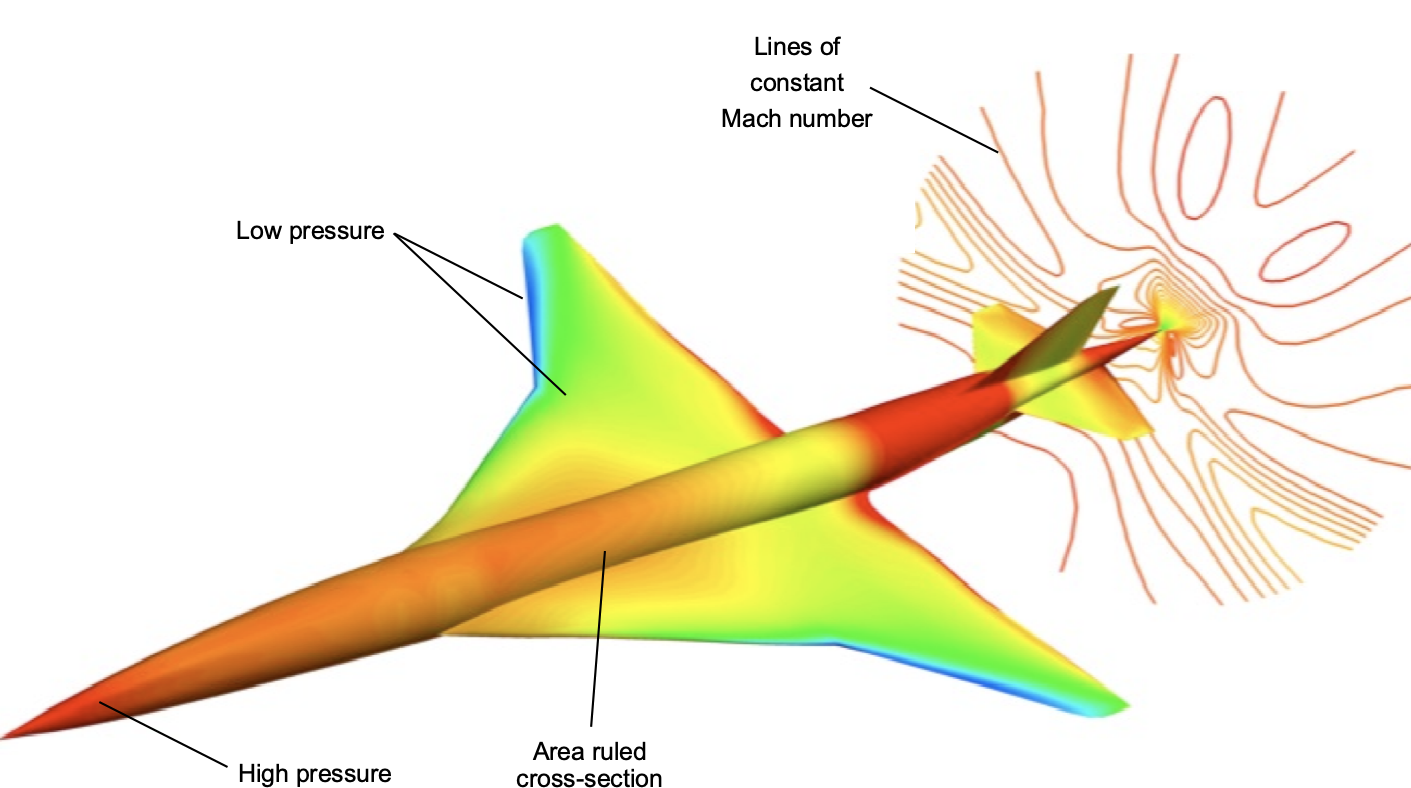


 is the flow density and
  ,
,  , is the velocity vector. For an incompressible flow, where


 is the pressure,
  is the stress tensor, and
  is a body force per unit mass, e.g., acceleration under gravity.
 is the Kronecker delta function, i.e.,
  for
for  , and
, and  otherwise, and
  is the coefficient of dynamic viscosity. The parameter
  is called the second coefficient of viscosity or bulk viscosity, usually given as
  , which is referred to as Stokes’s hypothesis.[7] The bulk viscosity, which can be measured, as can
  , then the term involving
  represents the rate at which the fluid’s density changes under compression or expansion. Therefore, the term
  in the stress tensor accounts for the viscous stresses arising from these volume changes.

 is the internal energy per unit mass,
  is temperature,
  is the bulk thermal conductivity, and
  is the external heat per unit mass. Finally, the ideal gas equation (equation of state) can be used to relate the thermodynamic quantities, i.e.,
 is the gas constant. Recall that the equation of state is one of the few truly “handy” equations in aerodynamics.
 is the conserved variable vector and
  ,
,  , and
, and  are the flux vectors. The flux vectors express the rate at which mass, momentum, and energy are transported at any flow point. This latter equation is often expanded into a form with the viscous terms on the right-hand side to give
 ,
,  , and
, and  are the fluxes resulting from the viscosity of the flow.
 and
and  directions are neglected to give
 , that accounts for the neglected
  derivatives.

 represents the external body forces per unit mass.

 and
and  are the mean (time-averaged) components, while
  and
and  are the fluctuating components, as illustrated in the figure below.
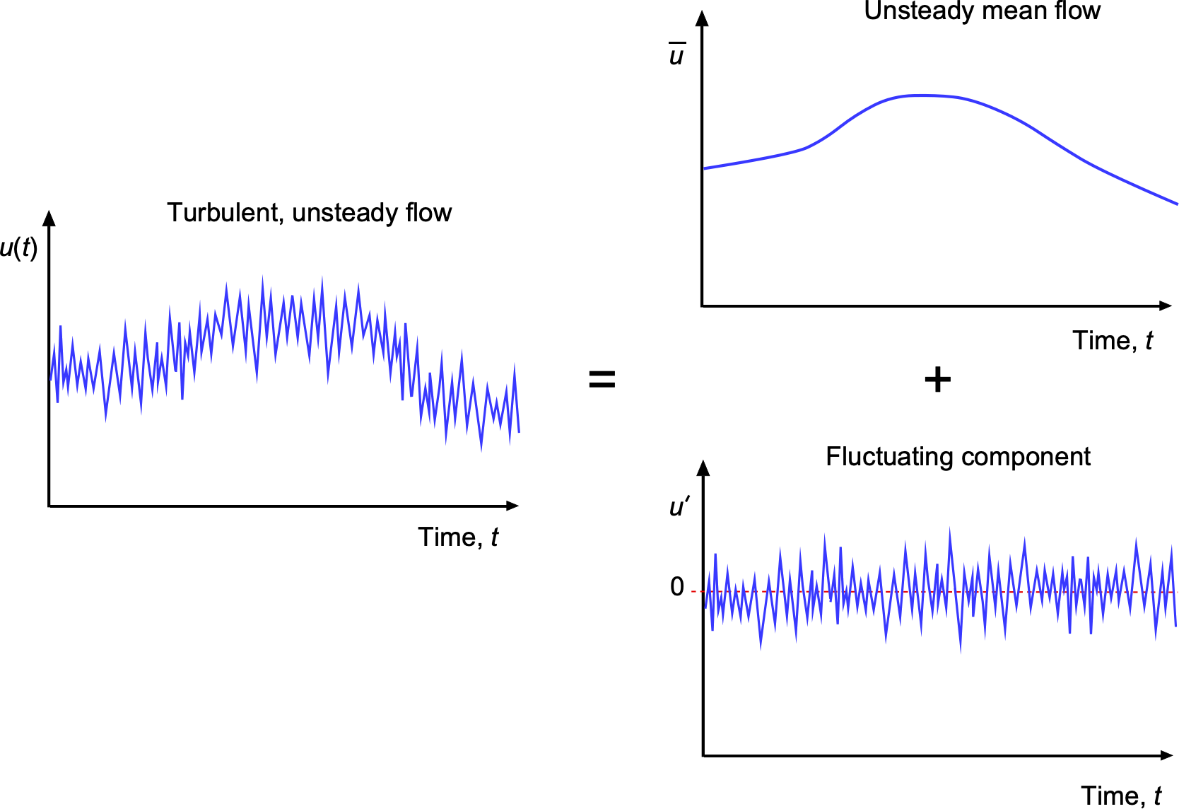
 introduces additional terms that account for the Reynolds stresses, which are the stresses created by the turbulent fluctuations. The averaged form of the continuity and momentum equations then becomes
 represents the divergence of the Reynolds stress tensor, which arises from the turbulent fluctuations. This term is often modeled using various turbulence models, which will be discussed later, because it cannot be directly calculated from the mean flow variables.
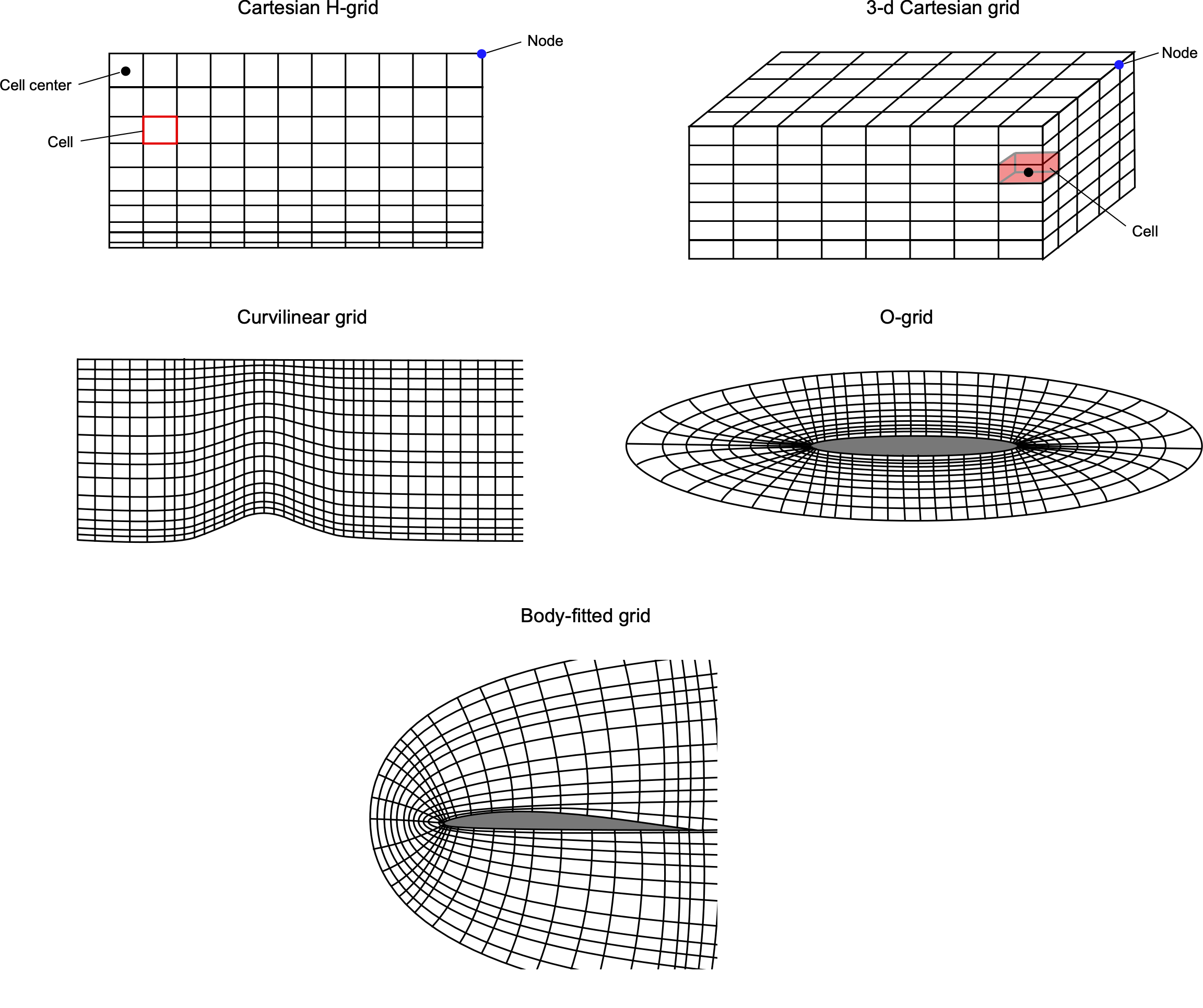
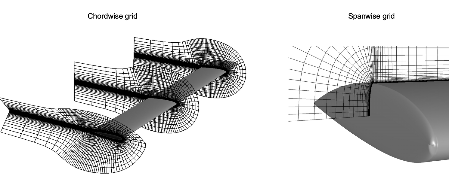
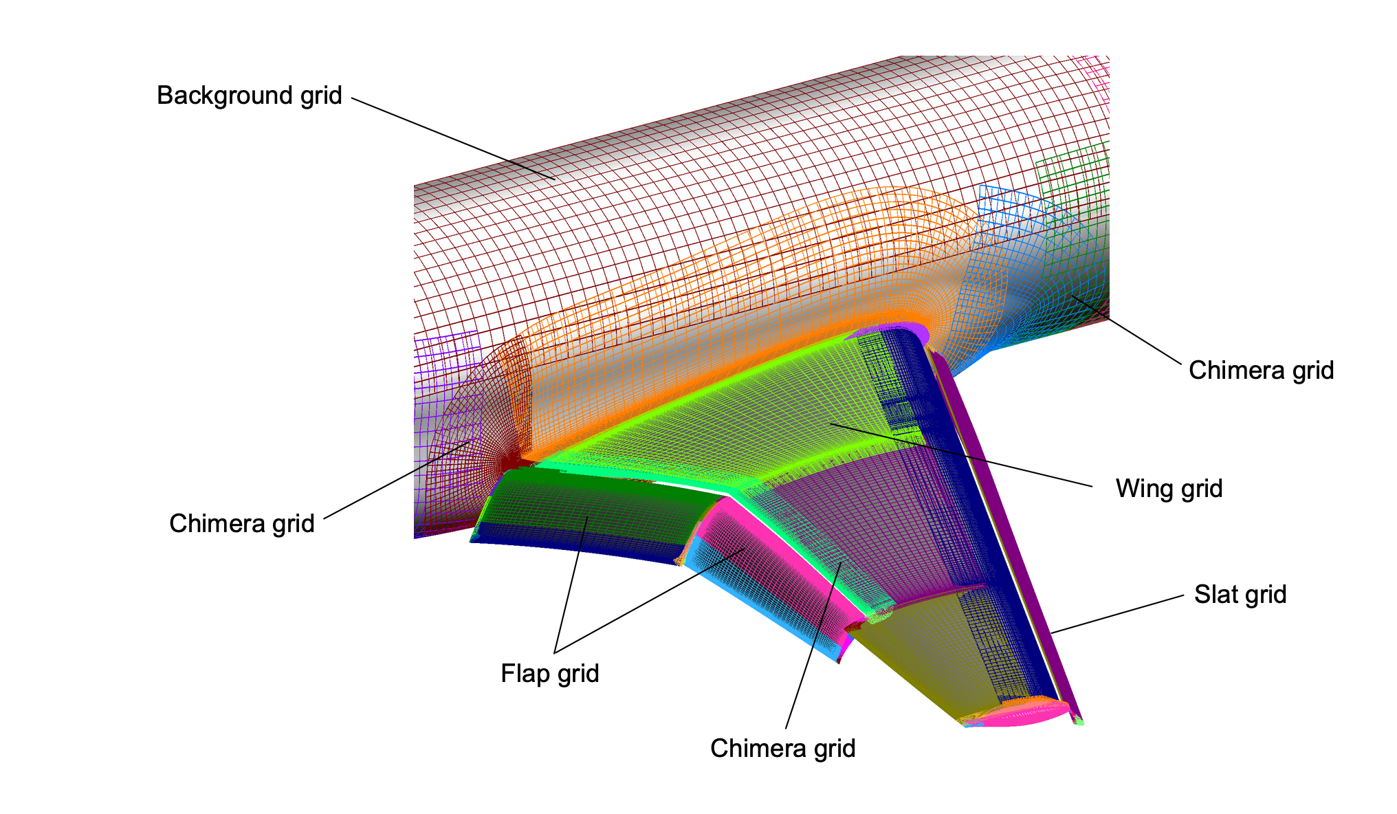
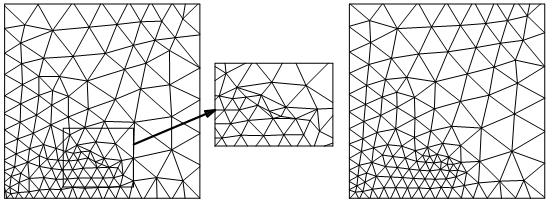

 . This latter formulation implies that
 is known as the eddy viscosity, representing an effective viscosity resulting from the effects of turbulence. Therefore, turbulence models that aim to simulate variations in eddy viscosity in the flow are called eddy viscosity models. In these models, higher levels of turbulent stresses are simulated by augmenting the effects of molecular viscosity alone with a turbulent viscosity coefficient, i.e.,
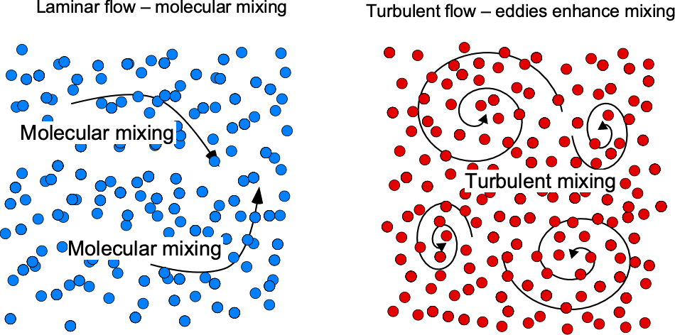

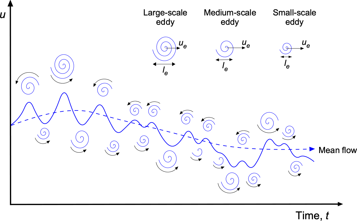
 models solve for two transport equations, one for the turbulent kinetic energy
  models also solve for two equations but use different variables, turbulent kinetic energy,
  , representing a generic scalar field that varies with space and time. For example,
 is the spatial discretization. The best way to understand this form of discretization is to use a stencil, as shown in the figure below. The nodes shown represent the four values in Eq.
  ,
,  ,
,  and
and  .
.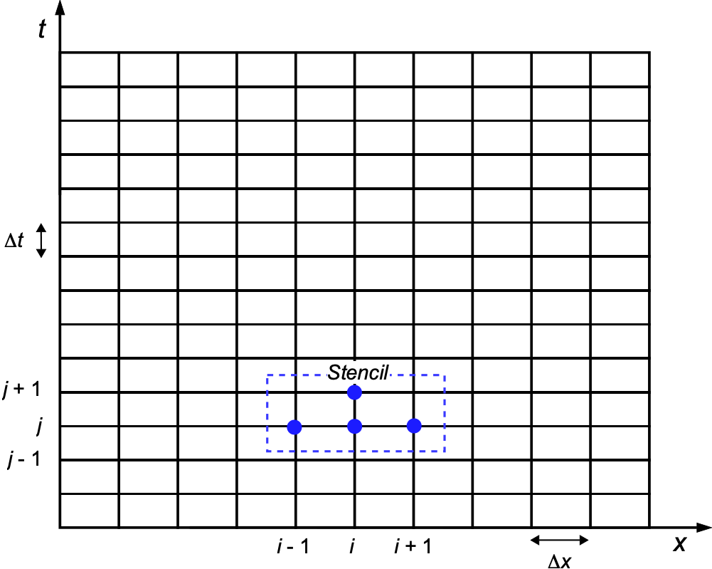


 . Higher-order differencing schemes can improve accuracy at the expense of more arithmetic operations and higher computer costs.
 is some constant. If
 is the temporal discretization. Using a central difference scheme for the spatial derivative gives


 is determined from the values at the previous time step
  .
. , can be populated. Applying the stencil further up the grid in time and across the physical space allows the values at step 4 to be obtained. The process can then be continued to cover the entire grid.
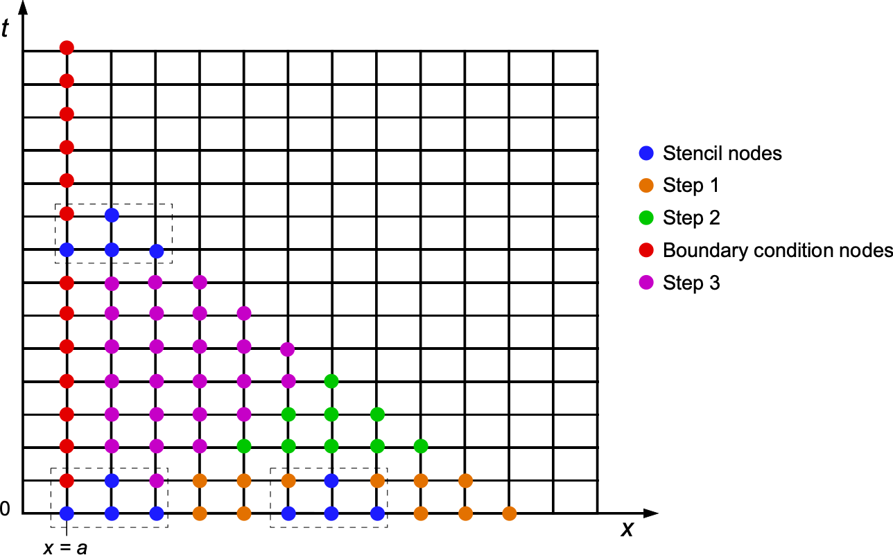
 control volumes, each with width


 , this latter equation must be integrated in time. For example, using an explicit forward difference method gives
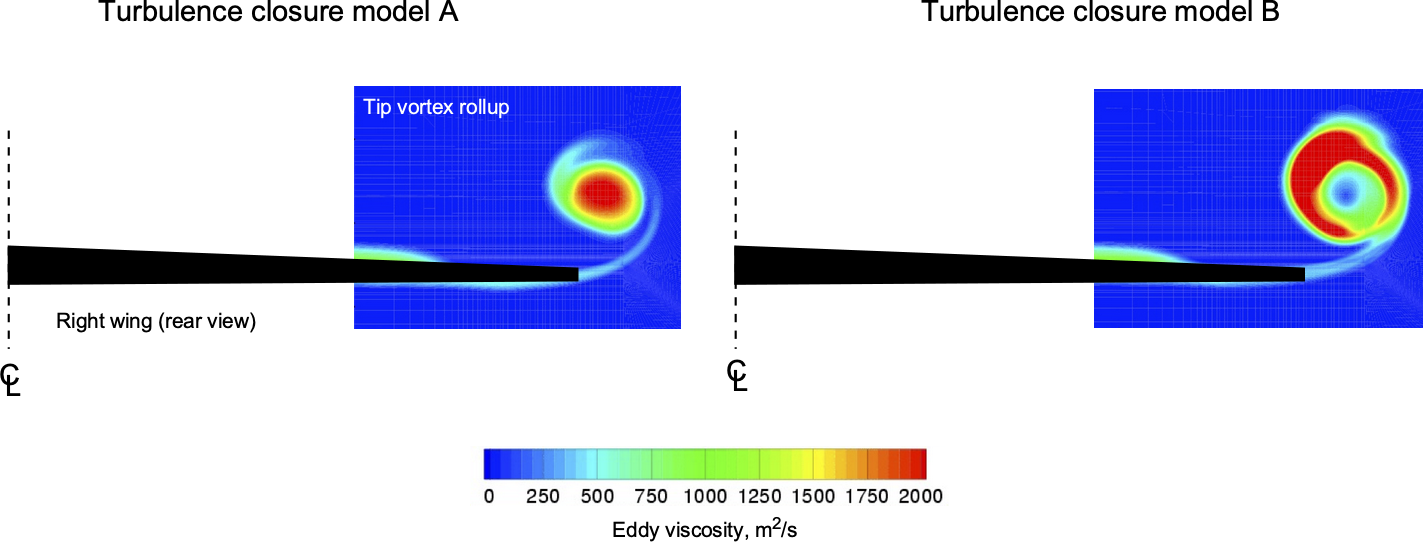


 ,
,  ,
,  , and
, and  represent the convective fluxes in the
  , respectively. The basic concept is shown in the figure below.
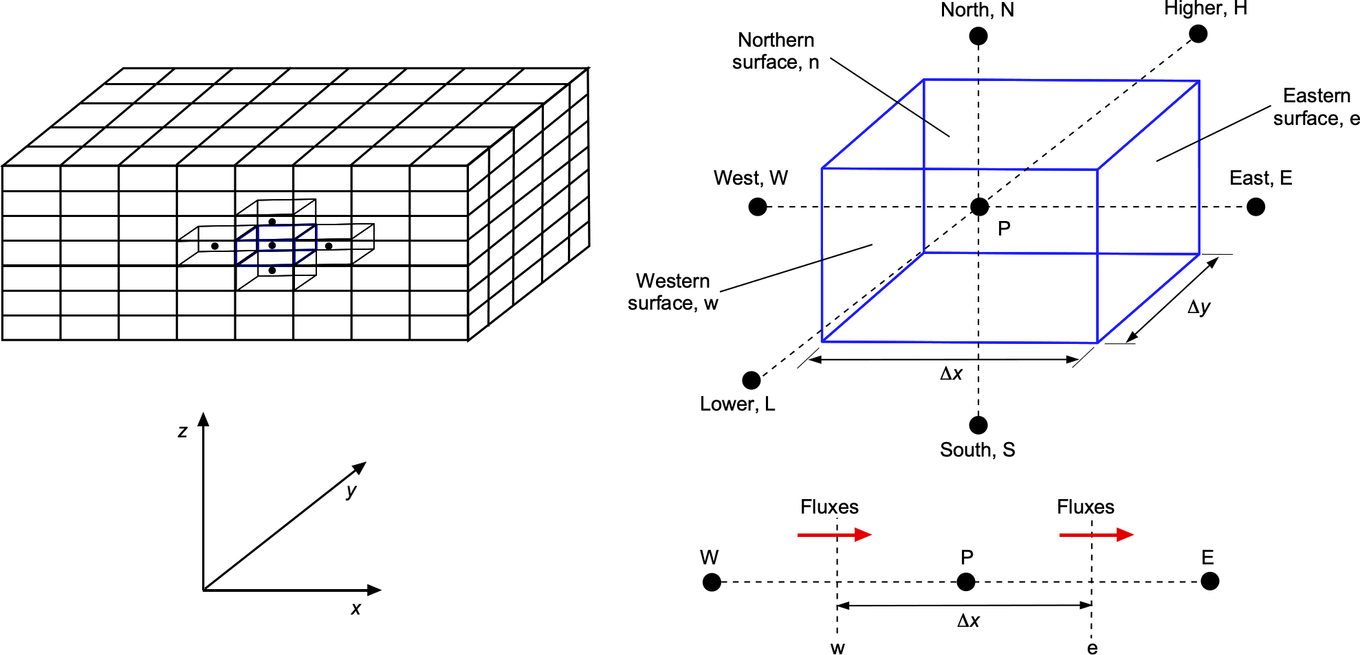


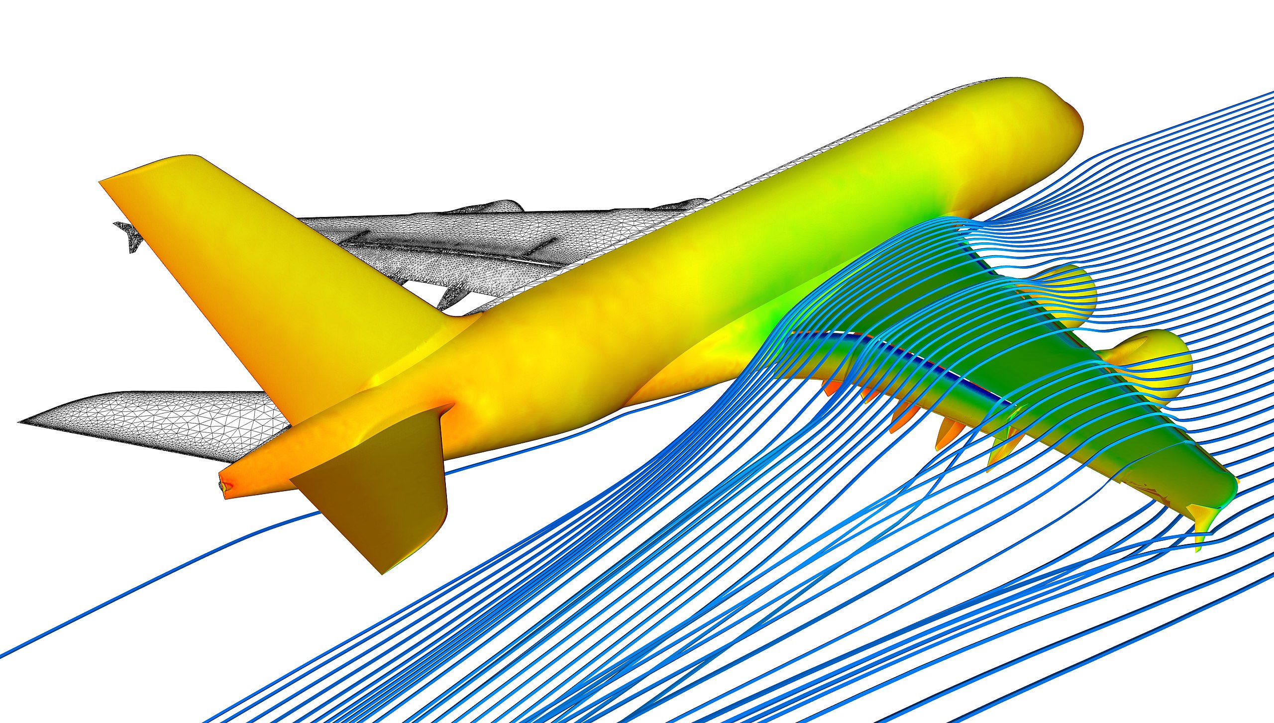
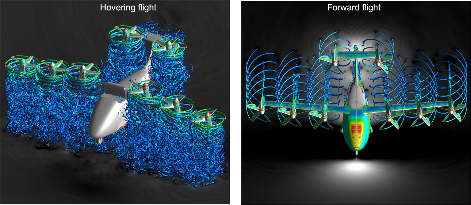


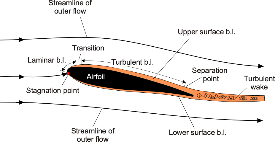
![\begin{eqnarray*} &&\frac{\partial u}{\partial x} + \frac{\partial v}{\partial y} = 0 \quad \hbox{(continuity)}\\[8pt] &&u \frac{\partial u}{\partial x} + v \frac{\partial u}{\partial y} = -\frac{1}{\varrho} \left( \frac{\partial p}{\partial x} \right) + \nu \frac{ \partial^2 u}{\partial y^2} \quad \hbox{(${x}$ component of momentum)} \end{eqnarray*}](https://eaglepubs.erau.edu/app/uploads/quicklatex/quicklatex.com-cdbf96c8fafb42fbab0bab9903d16a21_l3.svg "Rendered by QuickLaTeX.com")


 , where
  is the boundary layer thickness
 , which is defined as
 , yielding the same flow rate as in the viscous flow with the boundary layer present. This is equivalent to saying that the outer inviscid flow around the body can be obtained by solving the equations for a new shape obtained by adding the displacement thickness to the body’s actual shape. This approach is an example of a so-called weak interaction method. Although still an approximation, this approach yields more representative flow solutions than if the viscous effects were not included.
 is the shear stress on the wall (surface) and
  is the momentum thickness, given by
 . The irrotationality condition is a good assumption for external flows away from surfaces. In this case, the velocity field can be expressed as a gradient of a potential function,
![\begin{equation*} \nabla^2 \phi - \frac{1}{a^2} \left[ \frac{\partial^2 \phi}{\partial t^2} + \frac{\partial}{\partial t}(V^2) + \vec{V} \bigcdot \nabla \left( \frac{V^2}{2} \right) \right] = 0 \end{equation*}](https://eaglepubs.erau.edu/app/uploads/quicklatex/quicklatex.com-adc84539df125903ea49378265eaf3ff_l3.svg "Rendered by QuickLaTeX.com")
 . This form of the potential equation is usually called the full-potential equation because no terms have been neglected in its derivation from the Euler equation. For many flow problems, all the terms will be important if the characteristic nonlinear variation of the flow properties with Mach number is to be represented properly. However, other assumptions are possible.

 ,
,  , and
, and  , then


 represents a forcing term that refers to contributions that account for external influences or boundary conditions that modify the behavior of the flow.
![\[ \frac{\partial \phi}{\partial y} = \frac{\partial h}{\partial x} \]](https://eaglepubs.erau.edu/app/uploads/quicklatex/quicklatex.com-f98359c4c878572be97a17175f24ee3e_l3.svg "Rendered by QuickLaTeX.com")
 represents the airfoil’s thickness as a function of
  .
.![\[\phi(x, y, t) = \phi_s(x, y) + \phi_t(x, y, t)\]](https://eaglepubs.erau.edu/app/uploads/quicklatex/quicklatex.com-965971224908efa82c1923746643c6d1_l3.svg "Rendered by QuickLaTeX.com")
 accounts for the unsteady forcing because of the body’s motion.
 is the freestream speed of sound. In this simplified form, the equation describes the propagation of small disturbances in a compressible flow. This reduction to a wave equation is useful for understanding the basic characteristics of wave propagation in a fluid. It forms the basis for more complex analyses in transonic flow regimes. The full TSD equation includes additional nonlinear terms to account for the effects of transonic flow, but this simplified form captures the essence of wave propagation.
 ), in which case Laplace’s equation governs the velocity potential, i.e.,
 and
and  are solutions to the Laplace equation, then
  is also a solution. This property enables the construction of complex flow patterns by combining simpler solutions, such as uniform flow, sources, sinks, and vortices. The Laplace equation is the governing equation for incompressible flows and underlies what are known as surface singularity or “panel” methods.
 , which now depends on time
  . The instantaneous adaptation of the flow field to changes in boundary conditions results from the idealization of the infinite speed of sound in incompressible flow, meaning pressure disturbances propagate instantly to all parts of the flow field.
 contains a singularity distribution that can be described by a velocity potential function of unit strength
 must be found subject to the boundary condition that the flow must be tangential to the surface at
  on the surface, i.e.,
 is the outward pointing normal unit vector at the
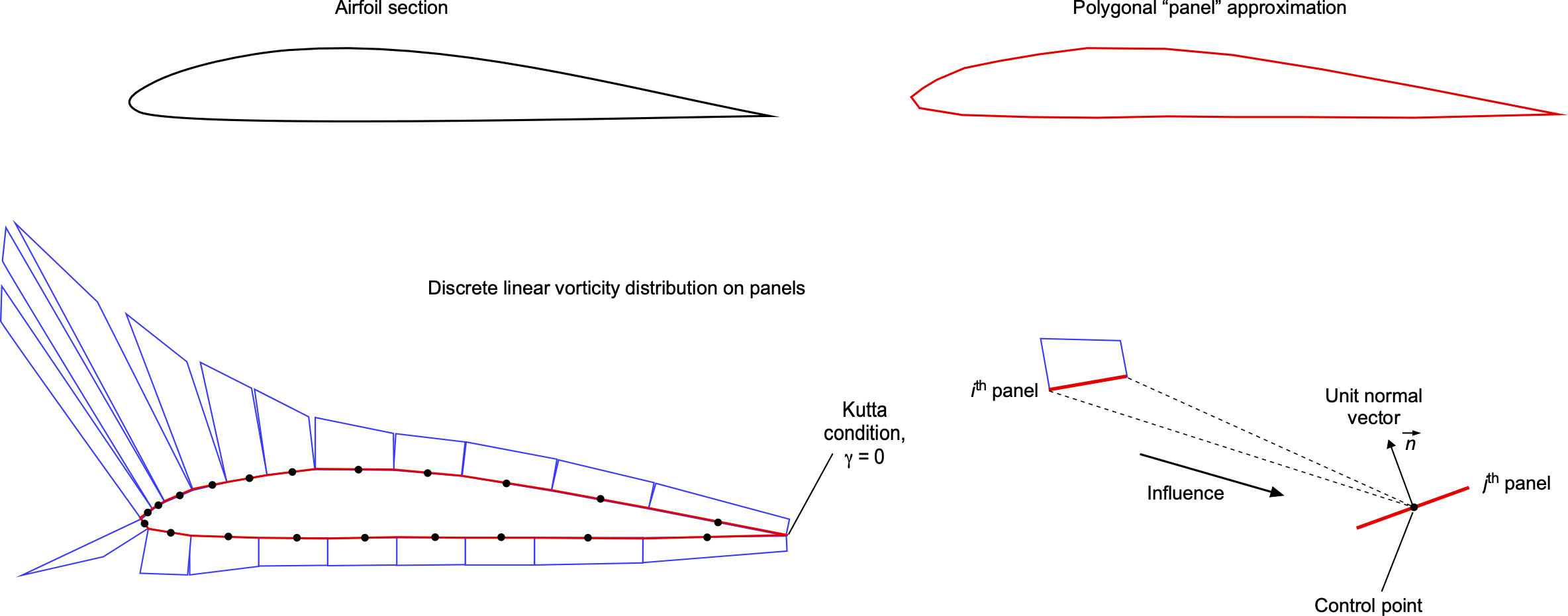
 unknowns. The
  , which is implemented by setting
  . Unless the Kutta condition is imposed in some form, the solution to the panel strengths becomes indeterminate. Therefore, the equations governing the problem can be expressed as
![\begin{equation*} \left\{ \begin{array}{c} \gamma_1 \\[6pt] \gamma_2 \\[6pt] \bigcdot \\[6pt] \bigcdot \\[6pt] \gamma_N \\[6pt] \gamma_{N+1} \end{array} \right\} = \left[ \begin{array}{ccccc} A_{1,1} & A_{1,2} & \bigcdot & \bigcdot & A_{1,N+1} \\[6pt] A_{2,1} & A_{2,2} & \bigcdot & \bigcdot & A_{2,N+1} \\[6pt] \bigcdot & \bigcdot & \bigcdot & \bigcdot & \bigcdot \\[6pt] \bigcdot & \bigcdot & \bigcdot & \bigcdot & \bigcdot \\[6pt] A_{N,1} & A_{N,2} & \bigcdot & \bigcdot & A_{N,N+1} \\[6pt] 1 & 0 & \bigcdot & 0 & 1 \end{array} \right]^{-1} \left\{ \begin{array}{c} -V_{\infty}\sin \alpha \bigcdot n_1 \\[6pt] -V_{\infty}\sin \alpha \bigcdot n_2 \\[6pt] \bigcdot \\[6pt] \bigcdot \\[6pt] -V_{\infty}\sin \alpha \bigcdot n_N \\[6pt] 0 \end{array} \right\} \end{equation*}](https://eaglepubs.erau.edu/app/uploads/quicklatex/quicklatex.com-26059f91a745a55e9cec4b6bebfbff1f_l3.svg "Rendered by QuickLaTeX.com")
 is a
is a  matrix of influence coefficients. An influence coefficient
  is effectively the normal component of the velocity induced at the collocation point on panel
  , then the velocity induced by this panel at the control point on the
  . At the
 is the velocity at panel
  , where
  is the unit normal vector to panel
![\begin{equation*} [ A_{ij} ] \{ \sigma_{i} \} = {-}\{\vec{V}_{\infty} \bigcdot n_{j} \}, \end{equation*}](https://eaglepubs.erau.edu/app/uploads/quicklatex/quicklatex.com-f51f9201ee838006f6a4cf79669403f3_l3.svg "Rendered by QuickLaTeX.com")
![\begin{equation*} \left\{ \sigma_{i} \right\} = \left[ A_{i,j} \right]^{-1} \left\{ -\vec{V}_{\infty} \bigcdot n_{j} \right\} \end{equation*}](https://eaglepubs.erau.edu/app/uploads/quicklatex/quicklatex.com-5e0dcaa39e5c6d714b708dccbcc96f27_l3.svg "Rendered by QuickLaTeX.com")
 are obtained, the velocity components tangential to the panels can be determined. Hence, the pressure distribution over the fuselage can be calculated using Bernoulli’s equation.
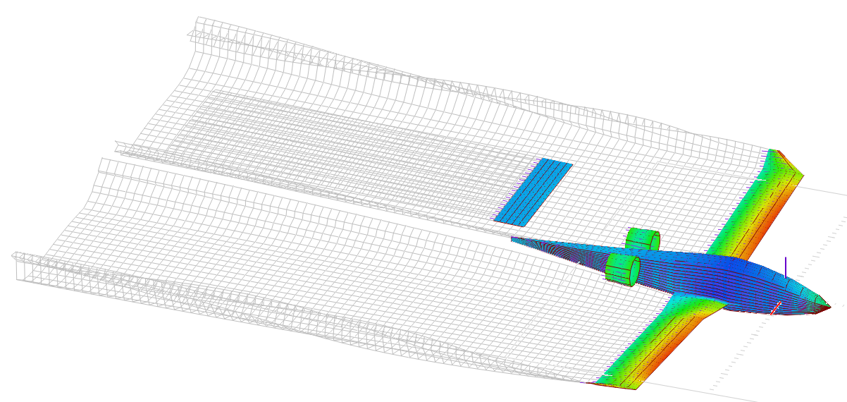
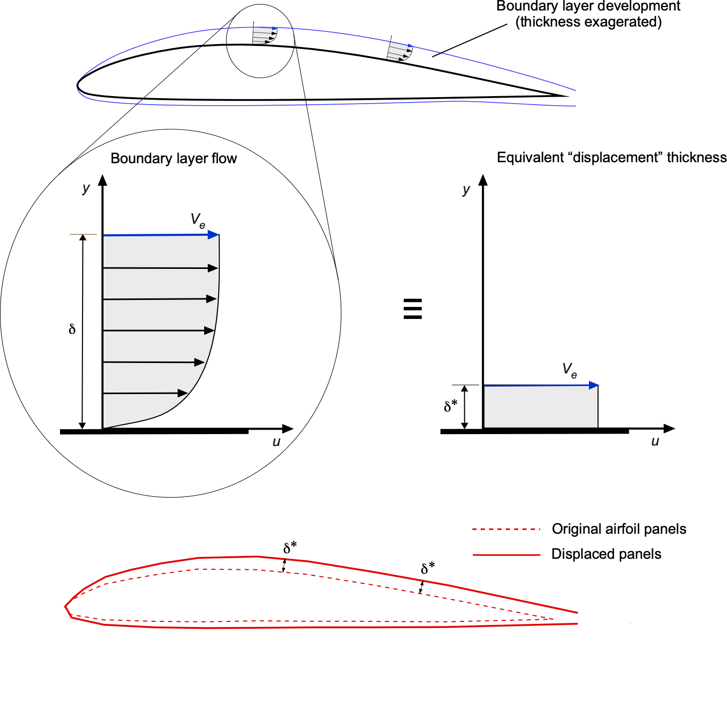
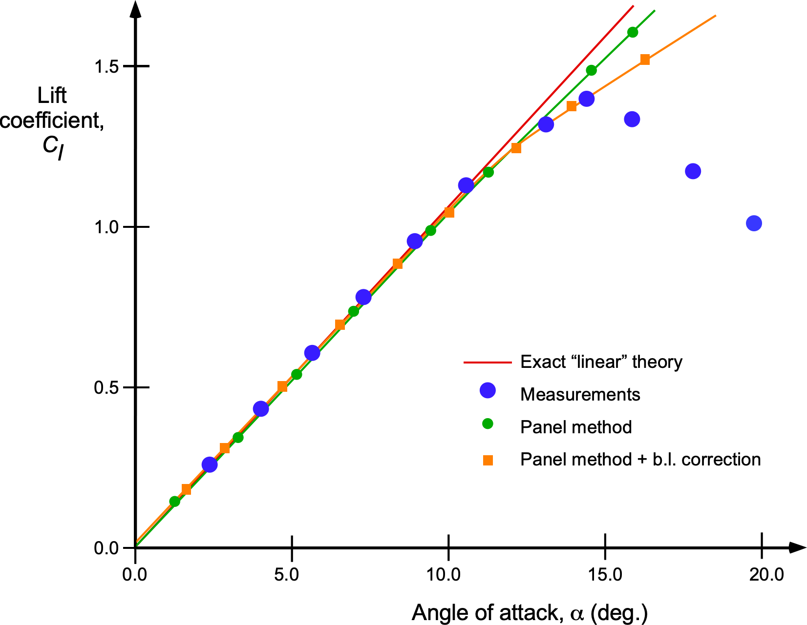
 , helps determine if a gas is rarefied or not, i.e.,
 is a characteristic length for the problem. If the value of
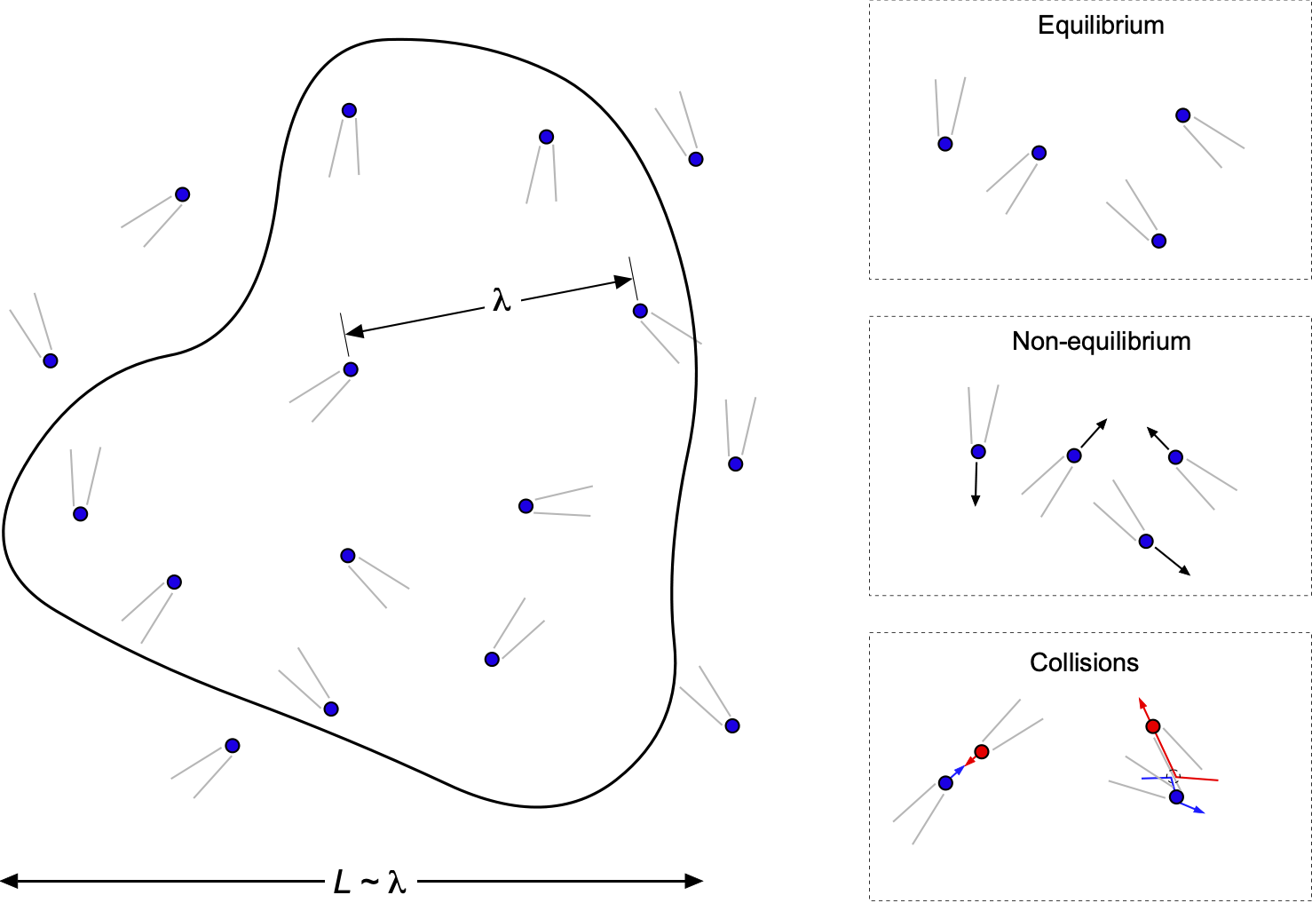

 is the
  is the mass of the gas molecule.
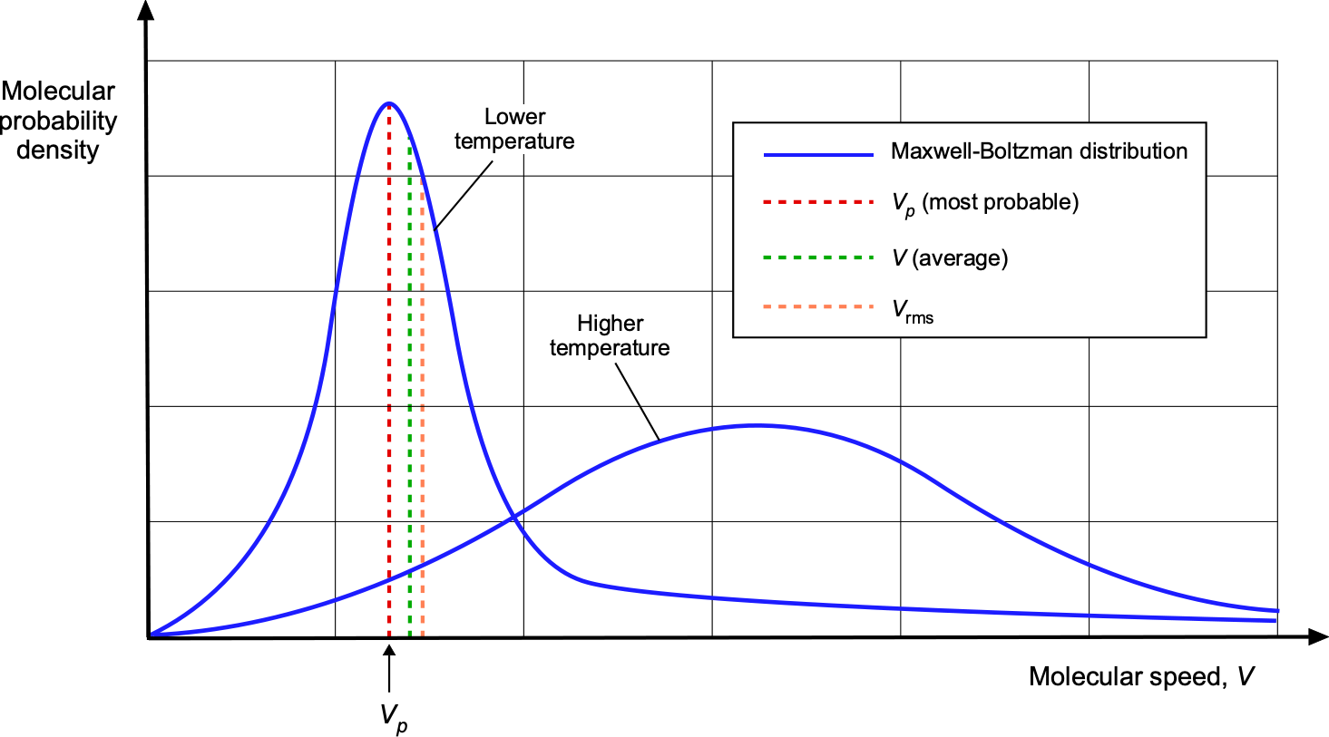
 Joules per Kelvin (J/K). At lower temperatures, the molecules have less energy. Therefore, the molecular speeds are lower, and the distribution is over a smaller range. As the temperature of the molecules increases, the probability distribution becomes more uniform because the molecules have greater energy at higher temperatures. So more of the molecules, on average, are moving faster. The average speed of all molecules is


 is the distribution function of molecules,
  is their velocity,
  is the equilibrium distribution, and
  is the relaxation time, i.e., the average time between molecular collisions. In a rarefied gas, this time is longer because the molecules are farther apart. Collisions between molecules drive the gas toward an equilibrium state, and models help account for these effects.
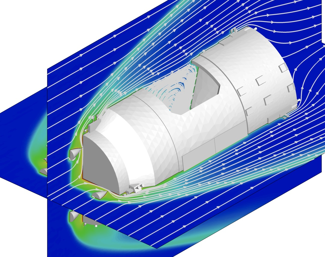
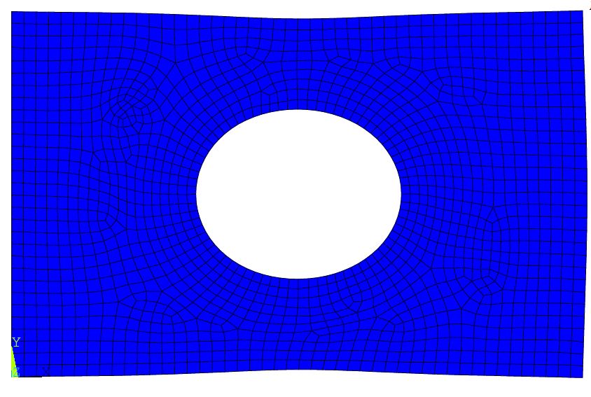
 elements with
  nodes, as illustrated in the figure below. The displacement within each element is approximated using shape functions
  and nodal displacements
  , i.e.,
 is given by
 is the strain-displacement matrix,
  is the material property matrix (e.g., containing Young’s modulus,
  , and Poisson’s ratio,
  ), and
  is the element’s spatial domain. The use of matrix multiplication in Eq.
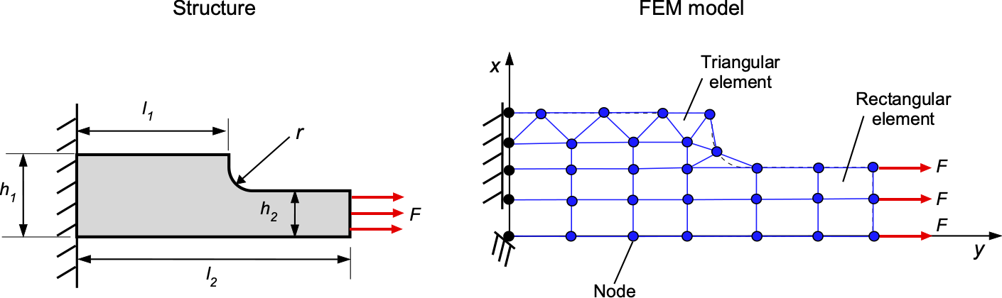
 is then assembled from the element stiffness matrices, i.e.,

 is the global displacement vector and
  is the global force vector. Boundary conditions are then applied to this system of equations. For an assembly of such elements, the global stiffness matrix
  efficiently, especially for large-scale problems, involves the use of various numerical methods.
 are linear for a triangular element with three nodes. Let the coordinates of the nodes be
  ,
,  , and
, and  , as shown in the figure below.
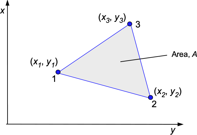


 ,
,  , and
, and  are determined by the coordinates of the nodes, i.e.,


![\begin{eqnarray*} \mathbf{B} = \begin{bmatrix} \dfrac{\partial N_1}{\partial x} & 0 & \dfrac{\partial N_2}{\partial x} & 0 & \dfrac{\partial N_3}{\partial x} & 0 \\[8pt] 0 & \dfrac{\partial N_1}{\partial y} & 0 & \dfrac{\partial N_2}{\partial y} & 0 & \dfrac{\partial N_3}{\partial y} \\[12pt] \dfrac{\partial N_1}{\partial y} & \dfrac{\partial N_1}{\partial x} & \dfrac{\partial N_2}{\partial y} & \dfrac{\partial N_2}{\partial x} & \dfrac{\partial N_3}{\partial y} & \dfrac{\partial N_3}{\partial x} \end{bmatrix} \end{eqnarray*}](https://eaglepubs.erau.edu/app/uploads/quicklatex/quicklatex.com-072c8a76fc3480678a4285f73314906e_l3.svg "Rendered by QuickLaTeX.com")

![\begin{equation*} \mathbf{B} = \frac{1}{2A} \begin{bmatrix} b_1 & 0 & b_2 & 0 & b_3 & 0 \\[6pt] 0 & c_1 & 0 & c_2 & 0 & c_3 \\[6pt] c_1 & b_1 & c_2 & b_2 & c_3 & b_3 \end{bmatrix} \end{equation*}](https://eaglepubs.erau.edu/app/uploads/quicklatex/quicklatex.com-2f26139f4437ac0447419b8c4e721432_l3.svg "Rendered by QuickLaTeX.com")
![\begin{equation*} \mathbf{D} = \frac{E}{1 - \nu^2} \begin{bmatrix} 1 & \nu & 0 \\[4pt] \nu & 1 & 0 \\[4pt] 0 & 0 & \dfrac{1 - \nu}{2} \end{bmatrix} \end{equation*}](https://eaglepubs.erau.edu/app/uploads/quicklatex/quicklatex.com-4106ecf3805ec6504c2d79fe47afa09f_l3.svg "Rendered by QuickLaTeX.com")


![\begin{equation*} \mathbf{K}^e = \left( \frac{1}{2A} \begin{bmatrix} b_1 & 0 & b_2 & 0 & b_3 & 0 \\[6pt] 0 & c_1 & 0 & c_2 & 0 & c_3 \\[6pt] c_1 & b_1 & c_2 & b_2 & c_3 & b_3 \end{bmatrix} \right)^T \left( \dfrac{E}{1 - \nu^2} \begin{bmatrix} 1 & \nu & 0 \\[6pt] \nu & 1 & 0 \\[6pt] 0 & 0 & \dfrac{1 - \nu}{2} \end{bmatrix} \right) \left( \frac{1}{2A} \begin{bmatrix} b_1 & 0 & b_2 & 0 & b_3 & 0 \\[6pt] 0 & c_1 & 0 & c_2 & 0 & c_3 \\[6pt] c_1 & b_1 & c_2 & b_2 & c_3 & b_3 \end{bmatrix} \right) \ A \end{equation*}](https://eaglepubs.erau.edu/app/uploads/quicklatex/quicklatex.com-86ed605d37632e66ac3369f436561d45_l3.svg "Rendered by QuickLaTeX.com")
![\begin{equation*} \mathbf{K}^e = \frac{E}{4A(1 - \nu^2)} \begin{bmatrix} b_1^2 + \nu c_1^2 & (1-\nu)b_1 c_1 & b_1 b_2 + \nu c_1 c_2 & (1-\nu)b_2 c_1 & b_1 b_3 + \nu c_1 c_3 & (1-\nu)b_3 c_1 \\[8pt] (1-\nu)b_1 c_1 & \nu b_1^2 + c_1^2 & (1-\nu)b_1 c_2 & b_1 b_2 + \nu c_1 c_2 & (1-\nu)b_1 c_3 & b_1 b_3 + \nu c_1 c_3 \\[8pt] b_1 b_2 + \nu c_1 c_2 & (1-\nu)b_1 c_2 & b_2^2 + \nu c_2^2 & (1-\nu)b_2 c_2 & b_2 b_3 + \nu c_2 c_3 & (1-\nu)b_3 c_2 \\[8pt] (1-\nu)b_2 c_1 & b_1 b_2 + \nu c_1 c_2 & (1-\nu)b_2 c_2 & \nu b_2^2 + c_2^2 & (1-\nu)b_2 c_3 & b_2 b_3 + \nu c_2 c_3 \\[8pt] b_1 b_3 + \nu c_1 c_3 & (1-\nu)b_1 c_3 & b_2 b_3 + \nu c_2 c_3 & (1-\nu)b_2 c_3 & b_3^2 + \nu c_3^2 & (1-\nu)b_3 c_3 \\[8pt] (1-\nu)b_3 c_1 & b_1 b_3 + \nu c_1 c_3 & (1-\nu)b_3 c_2 & b_2 b_3 + \nu c_2 c_3 & (1-\nu)b_3 c_3 & \nu b_3^2 + c_3^2 \end{bmatrix} \end{equation*}](https://eaglepubs.erau.edu/app/uploads/quicklatex/quicklatex.com-96b281a4dc1bfa08a4007563eac46e72_l3.svg "Rendered by QuickLaTeX.com")
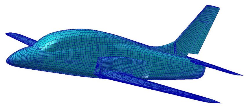
![\[ \left( \frac{\partial \phi}{\partial x} \right) + \left( \frac{ \partial \phi}{\partial y} \right) + \left( \frac{2}{\gamma - 1} \right) a^2 = \mbox{constant}, \]](https://eaglepubs.erau.edu/app/uploads/quicklatex/quicklatex.com-cd7f98bdc78194f0080ddd744c486b5e_l3.svg "Rendered by QuickLaTeX.com")
 , although later research suggests it is not always accurate. ↵
 . ↵
. ↵ ) exceeds that of an increase in the number of panels (order
  ). ↵
). ↵