59 Wind Tunnel Testing
Introduction
Wind tunnel testing remains a cornerstone of aerodynamic research for all types of flight vehicles. Wind tunnels come in various sizes and configurations, with test-section speeds ranging from subsonic to hypersonic. Their design and operation rely heavily on the principles of internal flows to ensure a clean, uniform, and steady flow environment in the test section. This controlled flow enables the systematic measurement of aerodynamic forces, surface pressures, and velocity fields on scaled wings, complete aircraft models, propellers, and other components. Accurate wind tunnel measurements are indispensable for validating design decisions and ensuring that predictive methods yield not only the correct results but also for the correct physical reasons.
Although a few basic wind tunnels had been built in the 19th century, the origins of modern wind tunnels and testing techniques can be traced to the Wright brothers’ 1901 wind tunnel. From this beginning, wind tunnel technology advanced rapidly in the early 20th century, including those designed by Gustave Eiffel and Ludwig Prandtl. Several national research institutions soon constructed increasingly capable facilities, such as those at the Royal Aircraft Establishment (RAE) in Britain, at AVA Göttingen, DFL Berlin-Adlershof, and LFA Völkenrode in Germany, and at the NACA in the United States. These facilities enabled pioneering research on compressibility effects in high-speed aerodynamics and on wings, as well as large-scale aircraft testing. By mid-century, wind tunnels had become indispensable to both research and industry, with specialized facilities supporting the study of supersonic and hypersonic missiles, reentry vehicles, and propulsion systems. For the following decades, advances in instrumentation expanded the range of measurable quantities, and optical diagnostics began to reveal the fine-scale structure of turbulence and flow separation.
In the 1980s, as computational fluid dynamics (CFD) emerged rapidly, some critics predicted the demise of the wind tunnel, suggesting that physical facilities could eventually be closed. With hindsight, the opposite has proven true. Rather than replacing wind tunnels, CFD has complemented them, with the two approaches (i.e., measurements versus computations) evolving into a highly synergistic paradigm. Wind tunnels remain indispensable for validation and calibration, especially in complex flow regimes where CFD still struggles, such as high-Reynolds-number separated flows, transition, and aeroelastic phenomena. Today, the field has come full circle, with modern research and development programs relying on a balanced combination of CFD and wind-tunnel data to ensure reliable aerodynamic predictions.
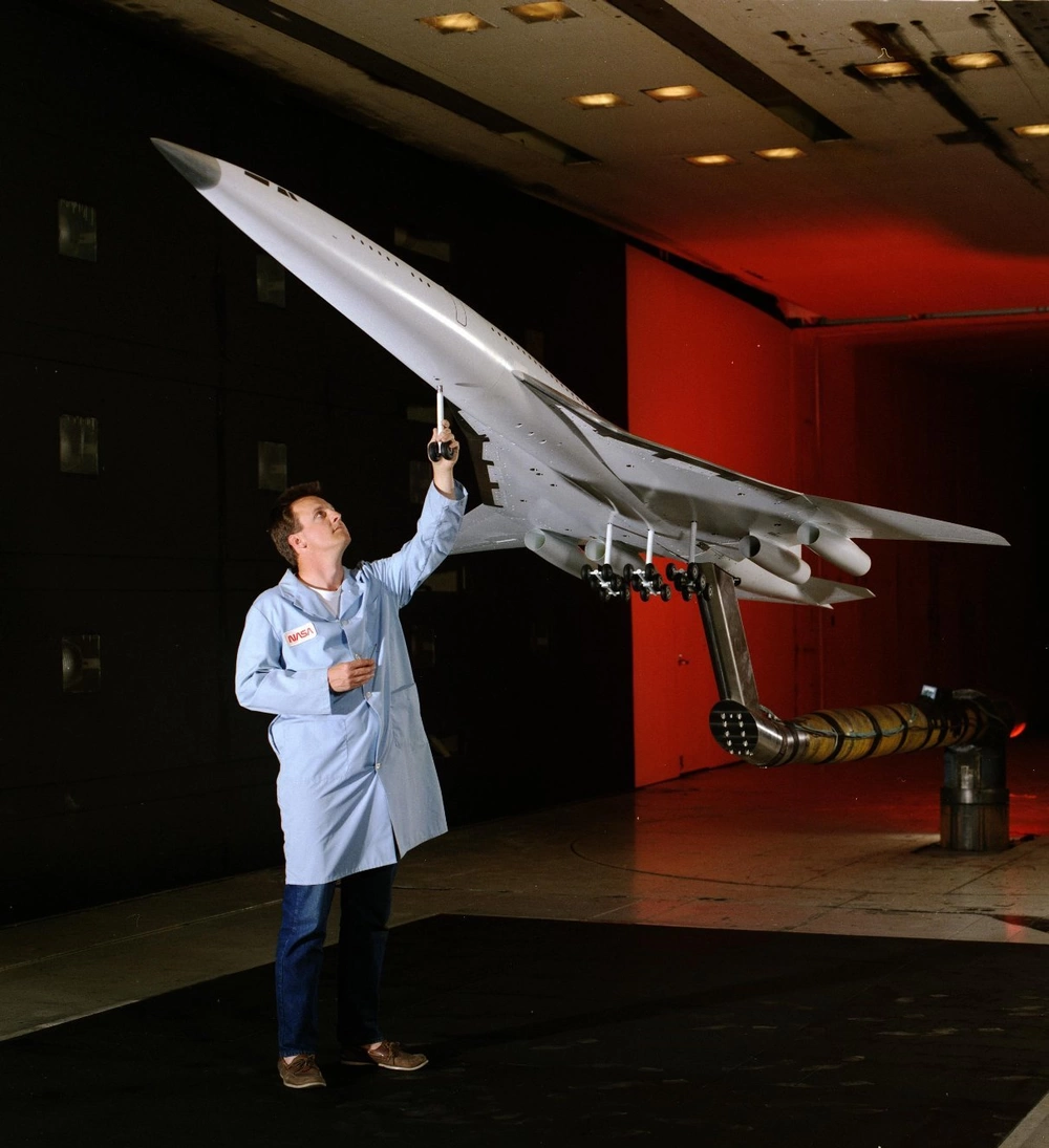
Over time, the applications of wind tunnels broadened well beyond aeronautics. Today, they are used in automotive and racecar design, wind turbine research, ship airwake studies, sports engineering, and civil engineering projects involving bridges, towers, and buildings. Their ability to generate controlled, repeatable flow fields makes them uniquely suited for both basic research and applied development across many disciplines beyond aerospace engineering. For example, the image below shows a 5-meter-diameter wind turbine being tested in the large 80-by-120-foot wind tunnel at NASA Ames Research Center.
Wind tunnels, therefore, remain an essential tool in the aerospace engineer’s repertoire, providing a controlled environment to investigate aerodynamic forces, flow behavior, and performance characteristics under simulated flight conditions. A solid understanding of their design features, capabilities, limitations, operational characteristics, and measurement methods is essential for all those working in experimental aerodynamics.
History
Before the advent of wind tunnels, free-flight and whirling arm devices were used to study aerodynamics. Free-flight tests, such as those conducted by George Cayley, provided no quantitative information, except for whether the concept flew well. Whirling arms rotated a test article through the air at the end of a long, cantilevered arm. Pioneered in the early 19th century by Francis Wenham, Horatio Phillips, and Hirium Maxum, these whirling rigs allowed them to measure lift on different bodies and surfaces, revealing key insights into the effects of angle of attack.
In Maxim’s design,[1] his wings and airplane designs were mounted on a set of “grocer’s scales” (i.e., a balance), and iron or lead weights were used until a pointer showed that the lift was precisely balanced. However, all such devices suffered from severe limitations, including three-dimensional and unsteady airflows and wake interference, which were shown to have provided misleading information.
The origins of wind tunnel testing date to the mid-19th century, when the limitations of free-flight experiments and whirling arms became increasingly apparent. Around 1871, under the auspices of the Aeronautical Society of Great Britain, the construction of what is now regarded as the first wind tunnel was led by Francis Wenham at Penn’s engineering works in England. This device consisted of a 10-foot-long (3.05-meter) rectangular duct with an 18-inch-square (0.46-meter-by-0.46-meter) cross-section. John Penn utilized one of his steam engines to power a fan, generating the necessary airflow.
Wenham used the tunnel to measure the lift and drag of various surfaces set at angles to the flow, demonstrating for the first time the aerodynamic benefits of longer, slender wings with high wingspans. Although the flow in this primitive wind tunnel was poorly characterized, it provided quantitative data on aerodynamic forces and, for the first time, shifted the study of flight toward a more scientific approach.
In the 1880s, Horatio Phillips constructed a wind tunnel with higher-quality airflow. The test section was 6 feet (1.8 meters) long, with a square cross-section measuring approximately 17 inches (43 centimeters) on each side. He placed a restrictor or contraction in the section, which caused the flow speed to reach up to 60 ft/s (18.3 m/s). The models were installed on a balance, which allowed measurements of lift and drag. Phillips studied cambered airfoils, though his results were reportedly of questionable quality. Nevertheless, he demonstrated the growing need for testing under controlled-flow conditions if aerodynamic behavior were ever to be understood.
During the same period, William Kernot and Nikolay Zhukovsky constructed small wind tunnels for aerodynamic testing. Zhukovsky’s 1891 tunnel enabled the investigation of airfoil shapes, especially the leading and trailing edge geometry, which led to the development of the circulation theory of lift.[2] This theory was to prove to be the foundation for many advances in the understanding of the aerodynamics of airfoils and wings.
In 1894, Hiram Maxim constructed a small wind tunnel with a square cross-section of 1.7 feet (0.52 meters) and a “contraction chamber” measuring 2 feet (0.61 meters) across. The airflow was generated by a pair of counter-rotating propellers powered by a 100 hp (75 kW) engine. To reduce turbulence, the flow passed through a series of flow-conditioning elements, including screens and guide vanes. The tunnel reportedly produced a relatively smooth flow at speeds up to 50 ft/s (22 m/s). The test models were mounted on a “mobile frame” equipped with mechanical scales, utilizing counterweights and levers, which enabled the measurement of lift and drag forces. Maxim’s reportedly higher quality experiments conclusively demonstrated the aerodynamic efficiency of higher-aspect-ratio wings and cambered airfoils.
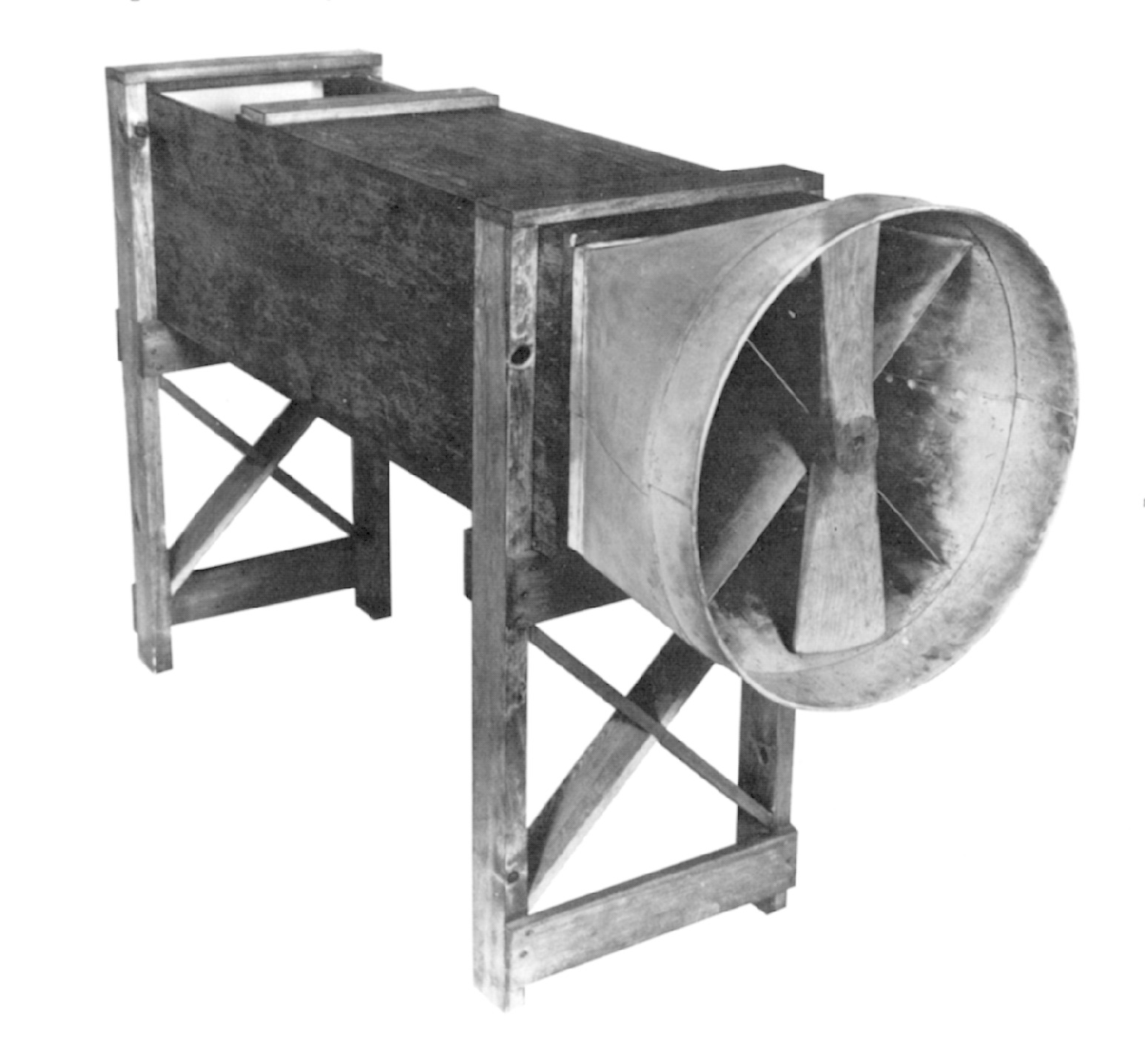
The Wright brothers’ 1901 wind tunnel marked a turning point in experimental aerodynamics. Dissatisfied with the poor performance of their gliders and the apparent inaccuracy of existing aerodynamic data,[3] The Wrights first mounted small test wings on their bicycles to measure lift and drag while riding, but this approach proved unsatisfactory. They then built a wind tunnel in their bicycle shop, about 6 feet (1.8 m) long, with a 16-inch-square (0.41 m × 0.41 m) test section. Using a balance of their own design, they carried out repeatable measurements of lift and drag on many wings and airfoil shapes.
Their systematic experiments confirmed the importance of aspect ratio, which directly led to the successful design of the 1902 glider and was a key feature critical to the success of the Wright Flyer of 1903. Equally important, their work introduced core testing principles such as geometric scaling, balances, and non-dimensional coefficients, together with validation through flight testing. Most will argue that their efforts marked a pivotal shift, firmly transforming the wind tunnel into a tool for aerodynamic analysis and engineering development.
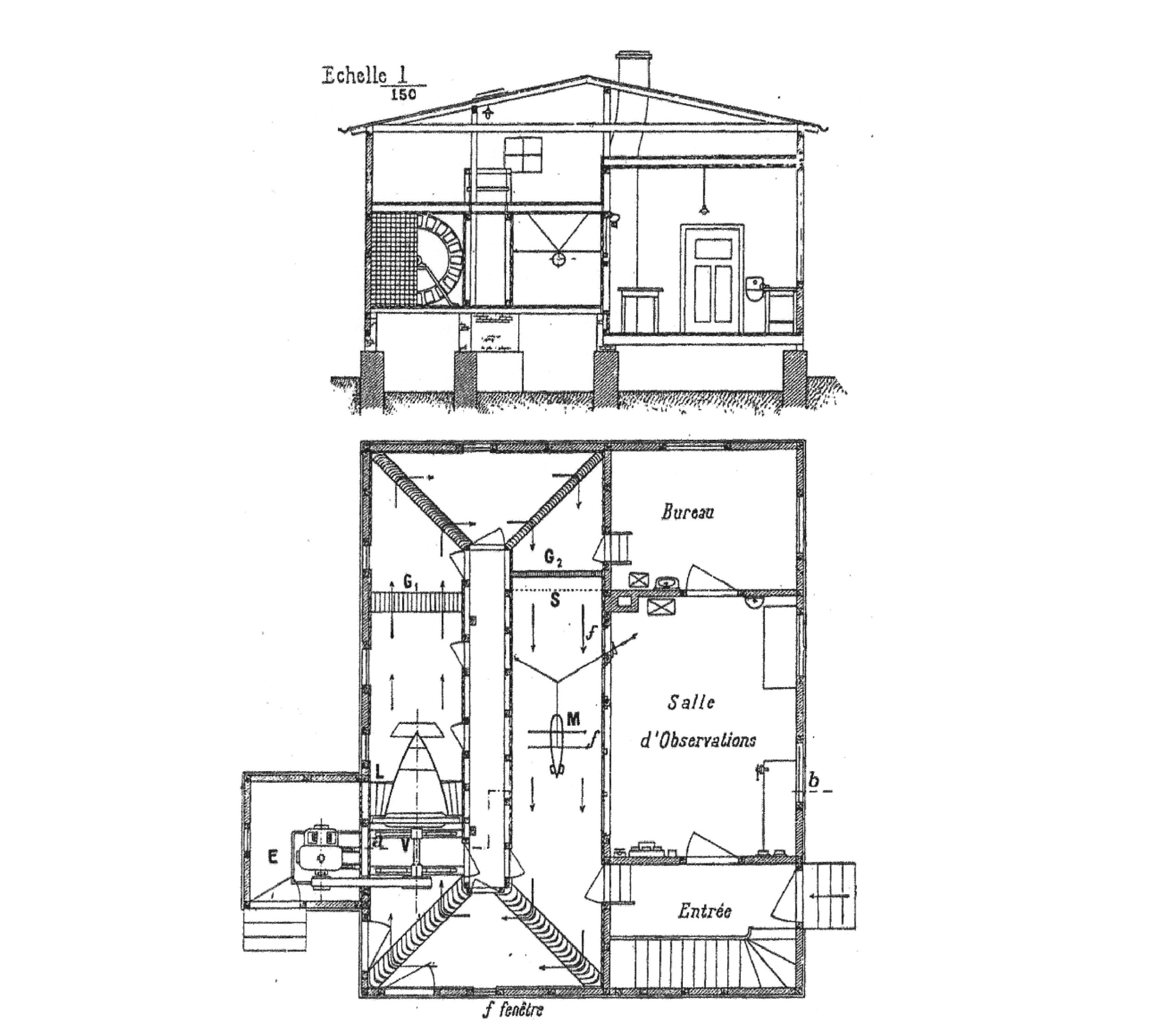
Another significant development in the development of wind tunnels occurred in 1909, when Gustave Eiffel constructed a compact wind tunnel near the Eiffel Tower in Paris. Motivated by a desire to understand the wind loads on large civil engineering structures, Eiffel developed an open-circuit, free-jet design with a carefully shaped converging nozzle and flow-straightening screens.
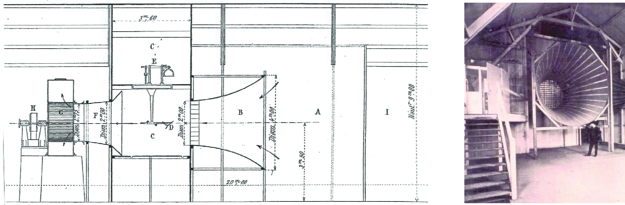
Eiffel’s instrumentation combined a force balance with distributed pressure taps. He was also the first to systematically test models of complete aircraft, introducing what he termed the “polar diagram,” a plot of lift and drag coefficients versus angle of attack that remains a standard form of aerodynamic analysis to this day. His 1912 tunnel had a test section of larger diameter and could reach higher flow speeds; his work helped further standardize aerodynamic testing procedures. By the 1920s, wind tunnel technology was rapidly maturing, and Eiffel’s wind tunnel design principles were widely adopted. New tunnels patterned after his design, commonly known to this day as the “Eiffel tunnel,” were being built worldwide to support the growing demands of aviation research.
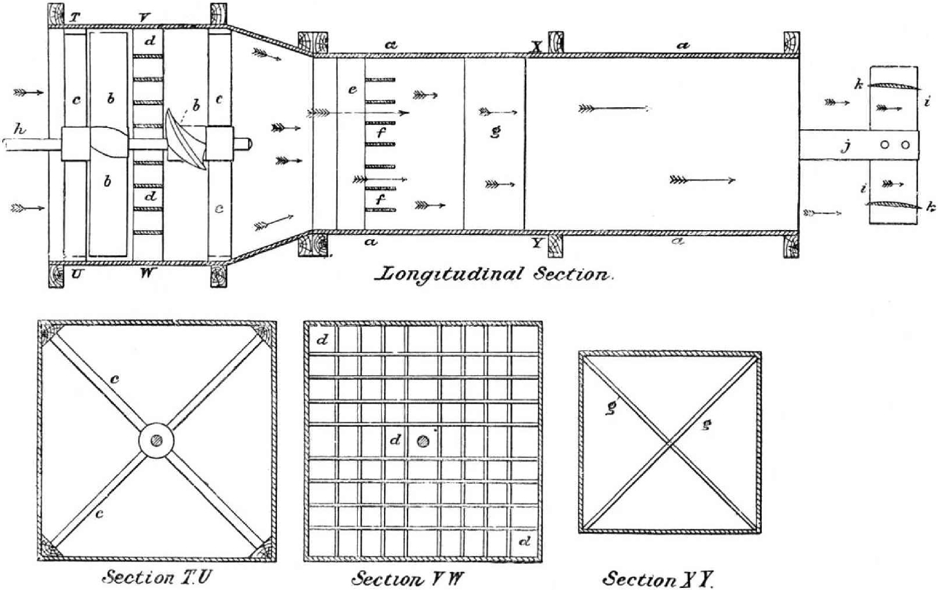
In 1909, Ludwig Prandtl introduced a fundamentally new wind tunnel configuration, namely the closed-return or closed-circuit wind tunnel. Prandtl’s design, which became known as the “Göttingen-type” wind tunnel, directed the flow in a loop, offering better energy efficiency and flow quality than the Eiffel tunnels. The corners featured turning airfoils or “vanes,” and a honeycomb screen was employed to straighten the flow at the inlet to the test section, thereby achieving greater flow uniformity and lower turbulence. Prandtl’s facility, shown in the drawing below, enabled more accurate measurements on airfoils, wings, and propellers. He and his students made many advances in understanding aerodynamics and laid the groundwork for further developments in wind tunnel testing methods.
National laboratories and major universities soon followed suit, building their own Eiffel- and Göttingen-type wind tunnels. These wind tunnels became standard tools in aircraft design, providing a means to test new configurations, refine airfoil sections and wing shapes, and investigate stability and control problems with a level of repeatability not possible through flight testing. By the end of the 1920s, most major aviation nations worldwide had established at least one significant wind tunnel facility. These early tunnels varied in size, flow speed, and design. Still, collectively they marked the transition from improvised testing and time-consuming flight testing to systematic aerodynamic measurements made under well-controlled conditions. They established foundational methods, including scale modeling, force-balance measurements, pressure measurements, and flow-visualization techniques, which led to explosive growth in the aerodynamic understanding of wings and airplanes.
By the early 1930s, the Royal Aircraft Establishment (RAE) was operating several large closed-return tunnels capable of high-quality integrated force and distributed pressure measurements on airfoils and complete aircraft configurations. The 24-foot (7.3-meter) tunnel and the 11.5-foot (3.5-meter) tunnel were particularly significant in advancing British aircraft design during the pre-war and WWII years. One of the most ambitious facilities was the RAE High-Speed Tunnel, designed to reach flow speeds of up to 880 ft/s (268 m/s, 600 mph, 965 kph) and operate under pressures ranging from one-fifth to four times atmospheric pressure. This wind tunnel played a central role in the development of high-speed aircraft. During the 1950s, it was modified to accommodate transonic flow testing, enabling experiments to be conducted over the Mach 0.9-1.15 range.
The NACA Variable Density Tunnel (VDT), completed in 1923 at Langley Field, used pressurized air at up to 20 atmospheres to achieve full-scale Reynolds numbers with subscale models. This innovation allowed unprecedented fidelity in low-speed aerodynamic testing. Notably, the VDT produced aerodynamic data[4] for many airfoil shapes. These data were used in the design of several airplanes of the time, including the Douglas DC-3, the Boeing B-17 Flying Fortress, and the Lockheed P-38 Lightning. Additionally, the VDT was used in testing the low-drag “laminar flow” airfoils employed in the wing design of the P-51 Mustang.
In the pre-war and WWII era, Germany established a network of advanced wind tunnel facilities that led aeronautical research in boundary-layer theory, compressibility effects, and swept-wing aerodynamics. The use of missiles and guided bombs during WWII sparked an interest in slender, supersonic configurations. These required more specialized wind tunnels to explore higher supersonic flight regimes and investigate frictional kinetic heating and shockwave drag. The research facilities at the Peenemünde Army Research Center included blowdown tunnels and expansion nozzles capable of reaching supersonic and hypersonic speeds up to Mach 7, enabling aerodynamic investigations of high-speed flight vehicles. After WWII, many of these German wind tunnels, which were well in advance of those elsewhere, were transferred to the U.K. and U.S. under Operation Paperclip, contributing to the development of high-speed wind tunnel testing facilities, including at the Arnold Engineering Development Complex (AEDC) and the Naval Ordinance Laboratory (NOL).
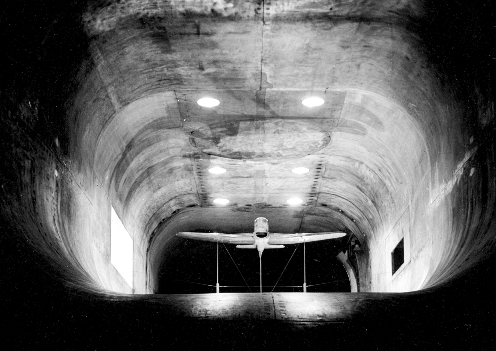
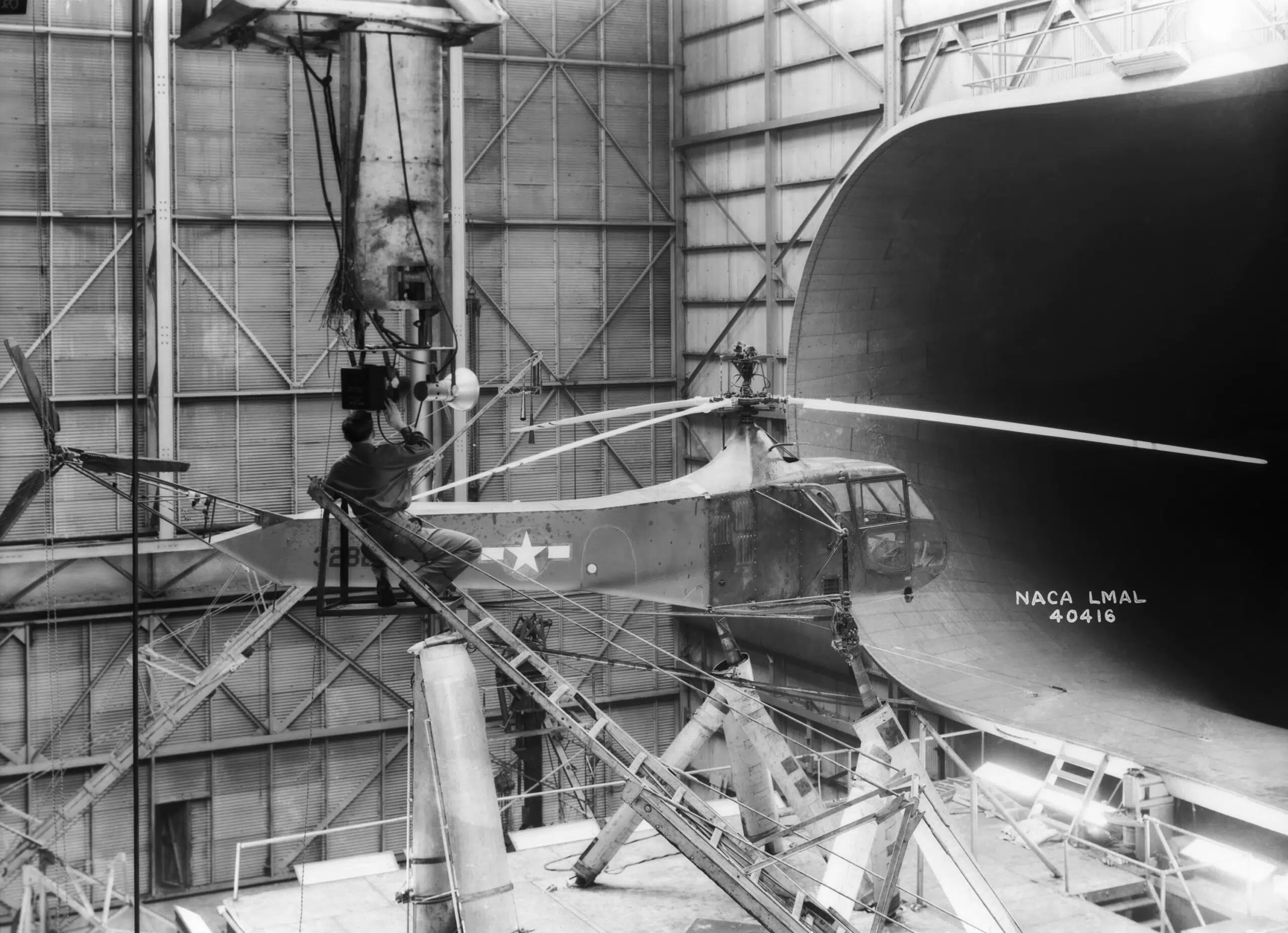
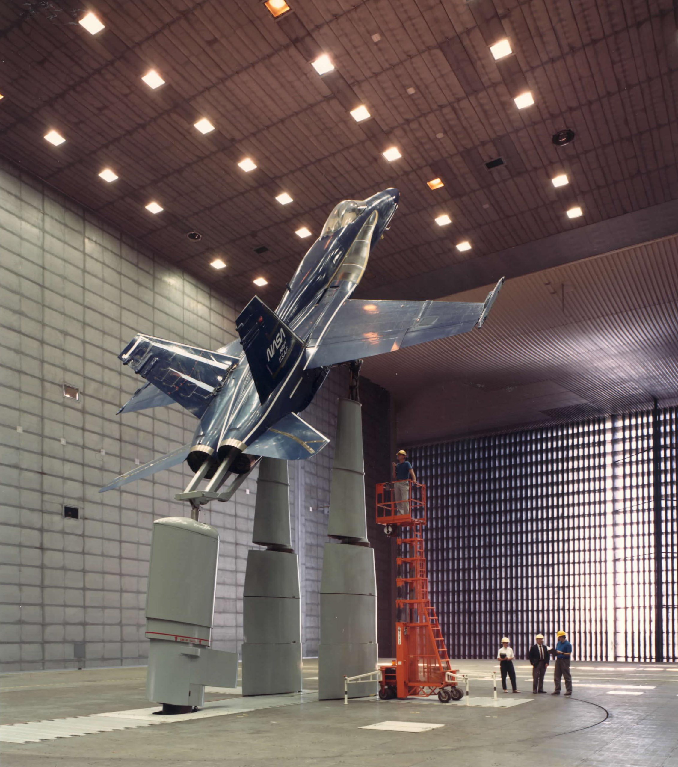
By 1931, NACA had constructed the 30-by-60-foot Full-Scale Tunnel, the largest low-speed wind tunnel ever built until the larger NACA 40-by-80-foot wind tunnel at NACA Ames was completed in 1949. It enabled full-scale aircraft tests, significantly improving the understanding of aerodynamic drag, stability, and control. Other NACA wind tunnels, such as the 7-by-10-Foot High-Speed Tunnel at Ames Research Center and the 16-Foot Transonic Tunnel at Langley, became central to much of the research. The 40-by-80-foot wind tunnel quickly became one of the most advanced in the world, capable of testing large test articles at low speeds, including full-scale airplanes, autogiros, and helicopters. A key feature was the nominally oval test section, which improved flow uniformity while minimizing wall interference.
The emergence of faster aircraft in the 1930s and 1940s brought new aerodynamic challenges. As speeds approached supersonic (Mach 1), compressibility effects, such as shock waves, associated flow separation, and flight control issues, became prominent. These phenomena could not be studied in existing wind tunnels, prompting the development of supersonic wind tunnel testing capabilities. The importance of these tunnels was underscored by the Bell X-1’s 1947 achievement of exceeding the Mach 1 “sound barrier,” which required an understanding of shock-wave development on the wings, gained through high-speed wind-tunnel testing.
In the postwar decades, attention also shifted to military airplanes capable of supersonic and, potentially, hypersonic flight, as well as to aeronautics and high-speed commercial airplanes. New research frontiers included thermal heating and shock-layer interactions. Hypersonic tunnels, typically ranging from Mach 5 to 15, were being built. These facilities presented many design challenges, including relatively short run times. The facilities included the AEDC von Kármán Gas Dynamics Facility, the Hypersonic Free Flight Tunnel at NASA Ames, and the shock-expansion tubes at NASA Langley Research Center and the California Institute of Technology (CalTech).
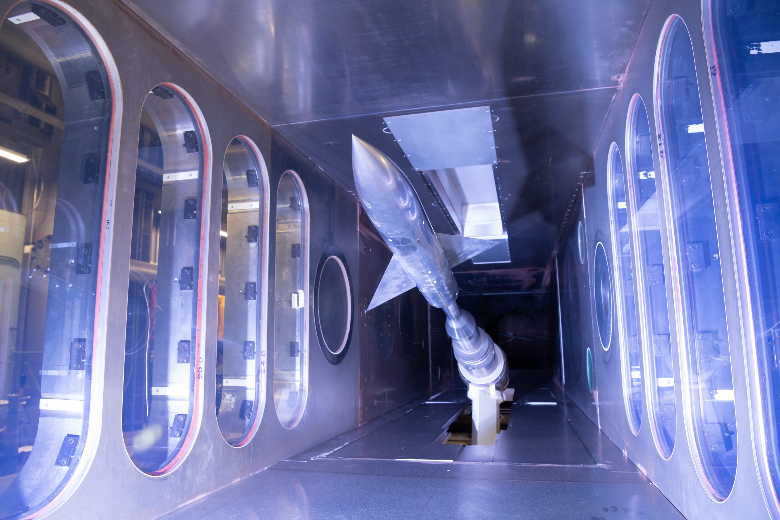
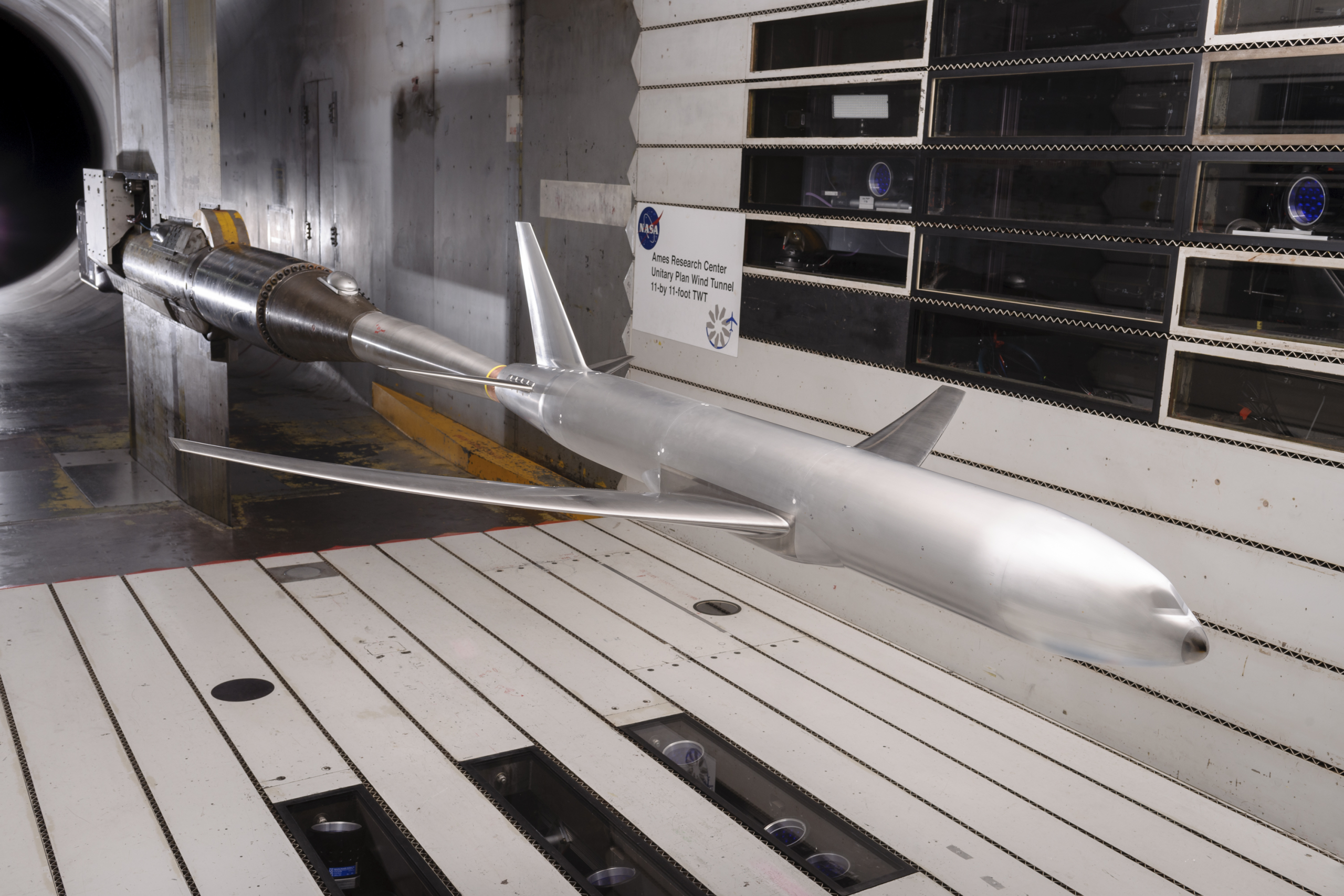
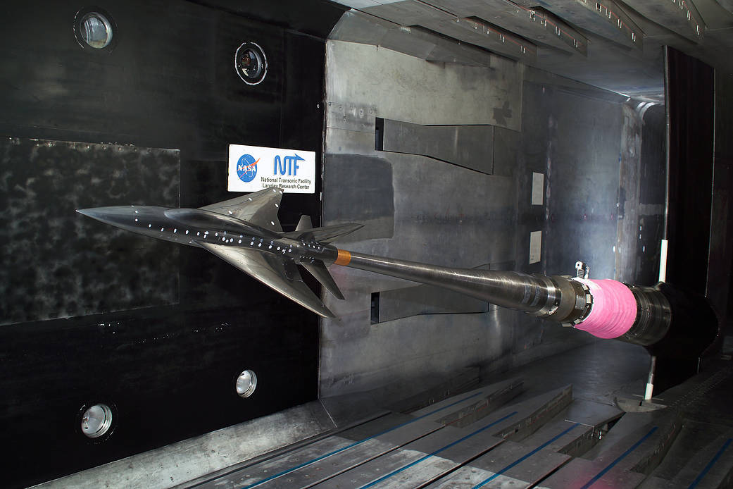
In the 21st century, wind tunnel facilities have adapted to new aerospace challenges, including electric propulsion, urban air mobility (UAM), drones, various new types of launch vehicles and spaceflight systems, and hypersonic vehicles. Modern wind tunnels are increasingly supporting joint studies where wind tunnel measurements are used in conjunction to help validate and improve high-fidelity CFD models. Cryogenic tunnels, adaptive wall designs, and automated test frameworks now extend the capabilities of even legacy infrastructure. NASA continues to modernize key assets such as the National Transonic Facility (NTF) and Unitary Plan Wind Tunnel (UPWT). A recent example of facility rejuvenation is the return to operation of the 11-Foot Transonic Wind Tunnel in 2022, which is one of three test sections within the UPWT complex, following extensive upgrades. This initiative reflects the trend of repurposing and modernizing legacy infrastructure rather than building entirely new wind tunnels.
The 80-by-120-foot wind tunnel at NASA Ames Research Center, part of the National Full-Scale Aerodynamics Complex (NFAC), was completed in 1982 as an expansion of the existing 40-by-80-foot (12.2-by-24.4-meter) tunnel. This addition was a key part of a comprehensive modernization project that began in 1972, aimed at enhancing the facility’s capacity to test larger aircraft and advanced aerospace systems. The updates included the installation of a new fan drive system, as well as the construction of the upstream 80-by-120-foot (24.4-by-36.6-meter) test section. With its combined test sections, the NFAC became the world’s largest wind tunnel facility, capable of testing full-scale airplanes and rotorcraft, and supporting critical aerospace research.
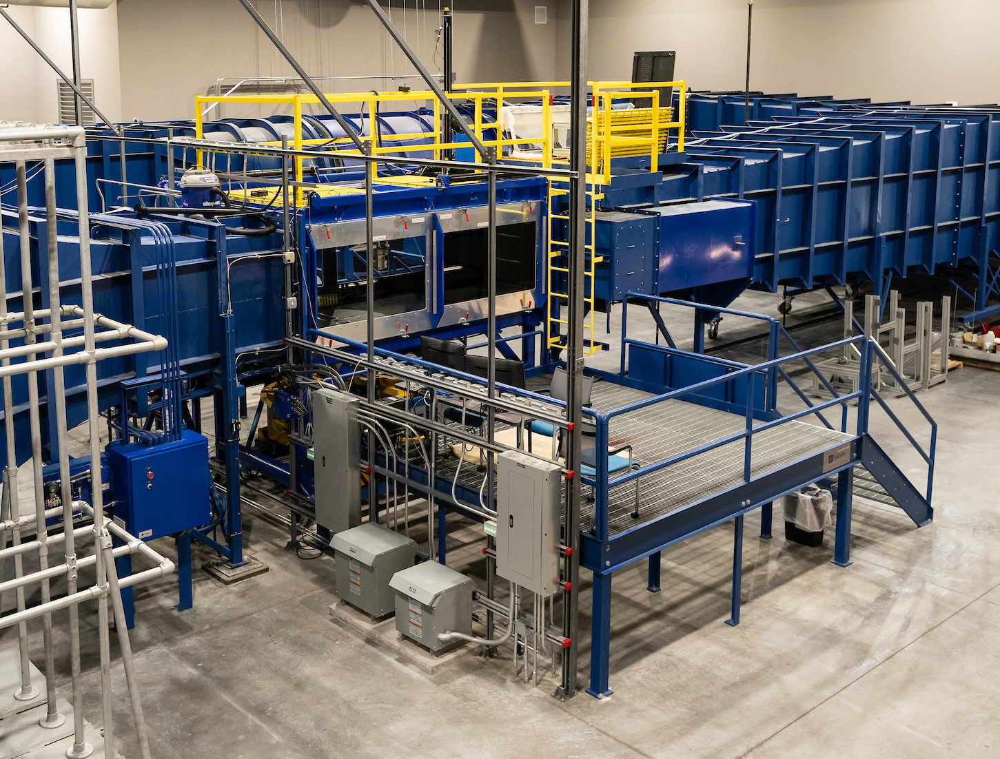
Apart from academic wind tunnels, new construction in the U.S. over the last decade has primarily focused on smaller-scale, high-speed tunnels for classified programs, particularly in hypersonics, for which few public details are available. One standout example of a modern academic wind tunnel is the Embry‑Riddle Aeronautical University’s Micaplex Low-Speed Wind Tunnel, completed in 2018 under the leadership of Professor J. Gordon Leishman. This closed-return, low-turbulence subsonic tunnel features a 4-by-6-by-12 ft (1.22-by-1.83-by-3.66 m) test section, with flow speeds of up to 250 mph (400 km/h), a six-component external force balance, and extensive optical access for PIV. The facility is used in research, undergraduate aerodynamics laboratories, and senior capstone projects. Another example is the recently rebuilt Wright Brothers Wind Tunnel at MIT, completed in 2021, under the leadership of Professor Mark Drela. The updated closed-circuit facility now features modern test instrumentation, increased test-section speeds, and enhanced flow quality.
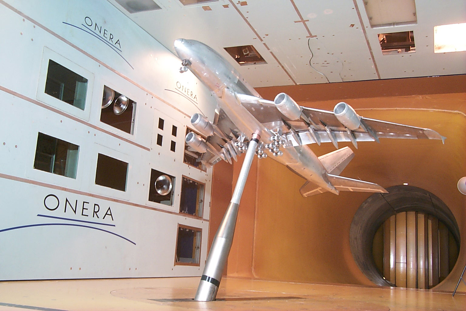
In Europe, ONERA’s S1MA tunnel remains one of the world’s most capable transonic facilities. DLR also operates advanced subsonic and hypersonic wind tunnels across multiple sites in Germany. In Asia, China’s JF-12 hypersonic shock tunnel is the world’s largest, and India’s DRDO and ISRO have expanded their test infrastructure for military and space applications. Australia’s University of Queensland maintains leadership in hypersonic aerothermodynamics with its X2 and X3 shock tunnels, while Japan’s JAXA and JAMSS support high-speed aerodynamic research using several specialized wind tunnel facilities.
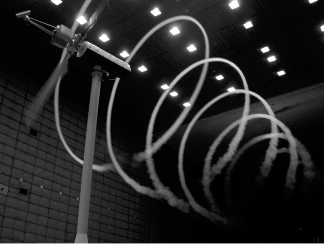
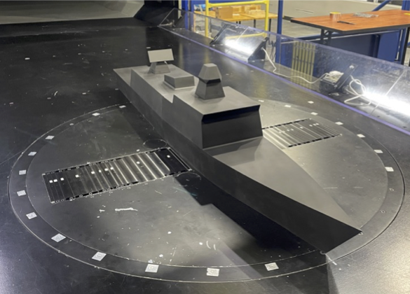
Today, wind tunnels span the full flight regime of aerospace flight vehicles. Subsonic tunnels support general aviation, rotorcraft, road vehicles, and many other applications, including ship airwake studies, as shown in the photograph below. Transonic tunnels are used to evaluate performance and analyze the onset of flutter in commercial airliners and other transport aircraft. Supersonic tunnels are used for the development of military aircraft, the integration of propulsion systems, and the testing of inlet performance. Hypersonic tunnels enable research on atmospheric entry vehicles, high-speed missiles, and air-breathing propulsion concepts. Despite the rise of high-fidelity CFD, wind tunnels remain indispensable. They provide valuable data for CFD validation, support the certification of flight vehicles, and offer insights into complex, unsteady phenomena that, for now, remain beyond confident computational capabilities.
Wind Tunnel Requirements
All wind tunnels have both general and specific requirements. In general, flow uniformity and long-term steadiness with low turbulence in the test section are critical to ensuring reliable test conditions. These requirements necessitate careful design of tunnel components to minimize turbulence intensity and flow angularity. Mach and Reynolds number scaling must also be addressed so that the flow behavior observed in the tunnel closely represents full-scale conditions.
More specific goals often involve adjusting model size, flow speeds, working fluid properties (in specialized facilities), or instrumentation requirements. In high-speed tunnels, precise control of pressure and temperature is essential for reproducing in-flight conditions. Large closed-return tunnels often incorporate cooling systems to dissipate excess heat generated by viscous losses as the flow circulates.
| Requirement | Description | Typical Target |
|---|---|---|
| Flow quality | The flow in the test section should remain uniform across the cross-section, steady over time, with very low turbulence and angularity. | Turbulence intensity < 0.1% (low-speed); angularity < 0.2°; velocity uniform to within 1–2% of mean; steadiness  0.1% over 10 s. 0.1% over 10 s. |
| Scaling | Conditions must approximate full scale through Mach and/or Reynolds similarity, sometimes requiring pressurization, cryogenics, or larger models. | Blockage ratio (frontal area of model to test section area)  0.05; confinement ratio (span of model to test section with or height) 0.05; confinement ratio (span of model to test section with or height)  0.7. 0.7. |
| Thermal control | Closed-return tunnels need cooling to remove heat; high-speed tunnels must regulate pressure and temperature precisely. | Temperature variation  across test section < 1 °C; stable pressure and temperature during runs. across test section < 1 °C; stable pressure and temperature during runs. |
| Acoustics & vibration | Noise and vibrations from the fan and drive system must not interfere with sensitive balances or instruments. | Balance platform vibration < 1  m; minimal acoustic spill into test section. m; minimal acoustic spill into test section. |
| Instrumentation | Balances, pressure sensors, and optical diagnostics such as PIV/DIC must be integrated with good optical access and proper laser measures. | Pressure resolution < 0.01% FS; synchronized data acquisition; clear reference frames and polarity conventions. |
| Repeatability | Key test points should be repeated to confirm stability of the data and tunnel conditions. | Force and moment repeatability < 0.1% of full scale (typical in low-speed tunnels). |
Acoustic and vibration isolation is also critical, particularly in high-speed or high-precision measurement applications. Mechanical noise and structural vibrations from the fan and drive motor can interfere with sensitive balances, which may need to be mounted on seismically isolated slabs. Supersonic or hypersonic tunnels are often built at remote facilities due to the high noise levels they generate.
Instrumentation and data acquisition systems in modern tunnels include sensitive pressure transducers, strain-gauge balances, and advanced optical diagnostics. In particular, optical systems such as Particle Image Velocimetry (PIV) must be integrated into the test section with sufficient optical access, along with strict safety measures for the use of high-powered lasers.
Types of Wind Tunnels
There are many different types of wind tunnels, although most fall into one particular category or classification. Even then, there is no “one size fits all” wind tunnel, and their specific design is directly related to the required speed of operation, size of the test articles, and instrumentation requirements, among other factors. Wind tunnels are generally classified by three primary criteria: speed regime, circuit configuration, and test section size, each reflecting specific design requirements and testing objectives. This systematic classification enables engineers to match the wind tunnel type to the type and size of the test article, as well as the aerodynamic phenomena being studied. For example, a model of a supersonic airplane would need to be tested in a wind tunnel capable of producing the appropriate range of supersonic flow in the test section and equipped with the proper instrumentation for measurements.
Subsonic Designs
Subsonic wind tunnels operate at Mach numbers below 0.3 and are primarily used to test general aviation aircraft, drones, automobiles, and civil engineering structures such as bridges and buildings. In this low-speed regime, compressibility effects are negligible. The primary design focus of subsonic tunnels is to achieve low turbulence intensity and a uniform velocity profile within the test section. Maintaining a steady, well-conditioned airflow over extended testing times is crucial for obtaining accurate aerodynamic measurements. These tunnels typically operate as continuous-flow facilities, using large fans to sustain the airflow. While the energy requirements are often modest compared to transonic or supersonic wind tunnels, continuous operation still entails significant overall power consumption. Nevertheless, the steady-state conditions that can be achieved allow for precise and repeatable measurements of aerodynamic forces, moments, and surface pressures.
Open-Circuit Designs
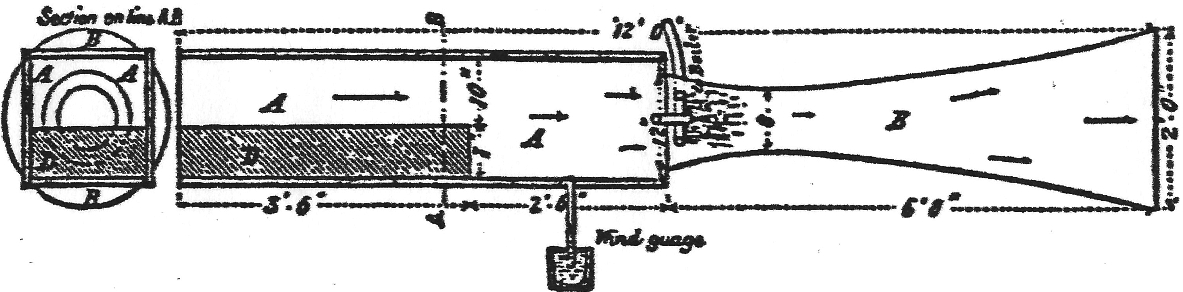
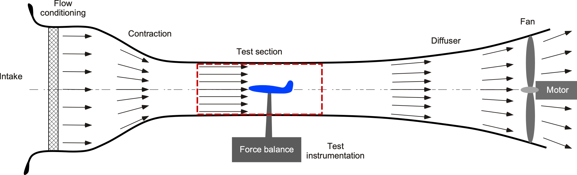
Open-circuit (Eiffel-type) wind tunnels draw in ambient air and exhaust it back into the environment, as illustrated in the schematic below. They are mechanically simple and inexpensive to construct and operate, typically consisting of a contraction section, a test section, and a diffuser leading to the fan outlet. Their main drawback is sensitivity to external conditions—any drafts, temperature gradients, or recirculating room air can disturb the inlet flow and increase turbulence levels in the test section. Consequently, these tunnels are not well-suited for precision aerodynamic measurements, and careful flow characterization is needed before they are used for quantitative testing.
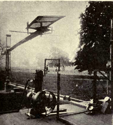
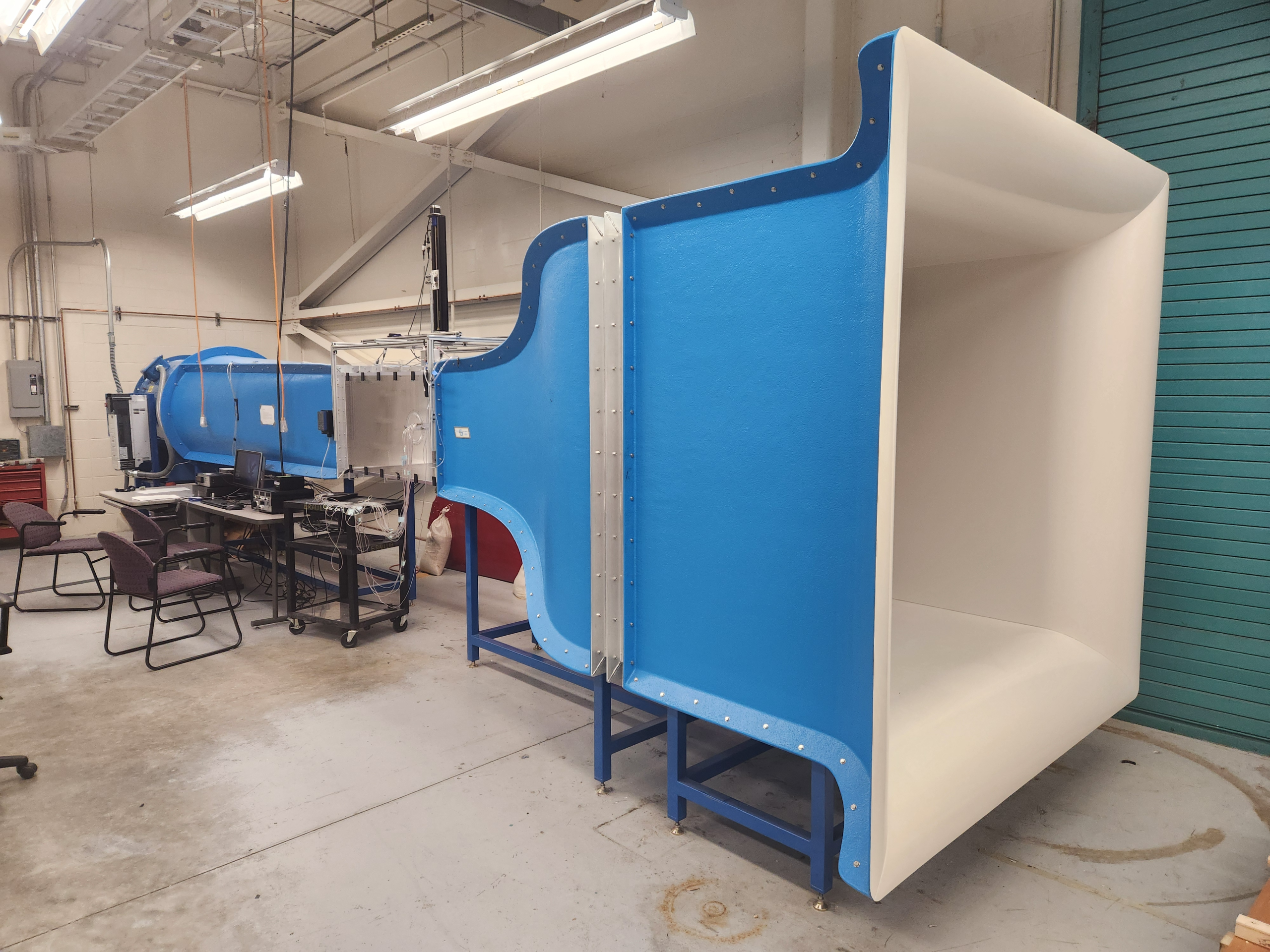
Nevertheless, open-circuit tunnels, as shown in the photograph below, remain widely used for instructional work and small experimental studies. Their low cost, simplicity, and accessibility make them ideal for student laboratories, where they provide hands-on experience in measuring aerodynamic forces, pressures, and flow patterns on different models.
Closed-Circuit Designs
Closed-circuit (Göttingen-type) wind tunnels recirculate the working air in a continuous, closed-loop configuration, as illustrated in the figure below. In this arrangement, the flow exiting the test section is guided through a system of turning vanes and diffusers. Then, energy is added by the drive fan before the flow completes the loop and re-enters the test section. Because the air’s properties remain within the circuit, external influences are significantly reduced. This approach not only improved flow quality but also allowed for precise control over key flow parameters, including velocity and temperature.
The recirculating nature of the design also improves energy efficiency, as the fan works to maintain flow against system losses rather than dissipating energy, unlike in open-circuit tunnels. Furthermore, noise levels are typically lower than in open-circuit designs, making the environment more suitable for sensitive instrumentation. For these reasons, closed-circuit wind tunnels are preferred in research and testing applications where high repeatability and measurement accuracy are essential.
Semi-Open Circuit Designs
Semi-open circuit wind tunnels incorporate features of both open-circuit and closed-circuit designs. In this configuration, a portion of the airflow is recirculated through the circuit, while the remainder is exchanged with the surrounding atmosphere. This hybrid approach reduces sensitivity to external environmental variations compared to a purely open-circuit Eiffel design, while avoiding the higher construction complexity and cost associated with a fully closed-circuit tunnel.
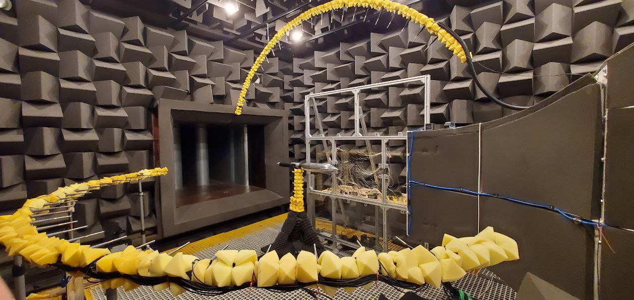
Semi-open tunnels have improved energy efficiency over open circuits while still maintaining easier access for test article changes and instrumentation. They are often selected for specialized applications, such as aeroacoustic testing, where the test section’s outer surfaces are lined with sound-absorbing materials to suppress reflections and enable accurate noise measurement, as shown in the photograph below. This feature makes them particularly suitable for evaluating propeller and helicopter rotor noise, fan blade tonal characteristics, and other unsteady aerodynamic phenomena where acoustic fidelity is essential.
Transonic Wind Tunnels
Transonic wind tunnels operate in the Mach number range of approximately 0.8 to 1.2, where compressibility effects become dominant and aerodynamic behavior changes rapidly with speed. In this regime, portions of the flow around a test article can accelerate locally to supersonic speeds, then abruptly decelerate through shock waves. These shocks can interact with the boundary layer, causing flow separation, buffeting, and other nonlinear phenomena that strongly influence the lift and drag on the test article.
To address these challenges, transonic tunnels are typically equipped with slotted or perforated test-section walls that allow a controlled amount of flow to pass through. This feature reduces the strength of shock wave reflections from the tunnel walls, thereby minimizing wall interference effects and providing more representative free-flight conditions. Advanced wind tunnel configurations may also incorporate adaptive wall technology to control blockage further and streamline curvature effects.
Because transonic flow is inherently complex, typically involving a combination of subsonic, sonic, and supersonic regions over the test article, such facilities are indispensable for understanding the aerodynamic intricacies that underpin the design of commercial transport aircraft, business jets, and certain military aircraft. They provide critical data for optimizing wing sweep, airfoil design, and control surface effectiveness in the speed range where shock-induced drag rises and changes in flight stability characteristics can significantly impact the overall performance of the flight vehicle.
Supersonic Wind Tunnels
Beyond Mach 1.2, where the flow about a body or aircraft is entirely supersonic, dedicated supersonic wind tunnels are required to reproduce the aerodynamic and thermodynamic conditions of high-speed flight. These facilities typically operate up to about Mach 4 or 5 and are designed to generate steady, uniform supersonic flows suitable for controlled aerodynamic testing.
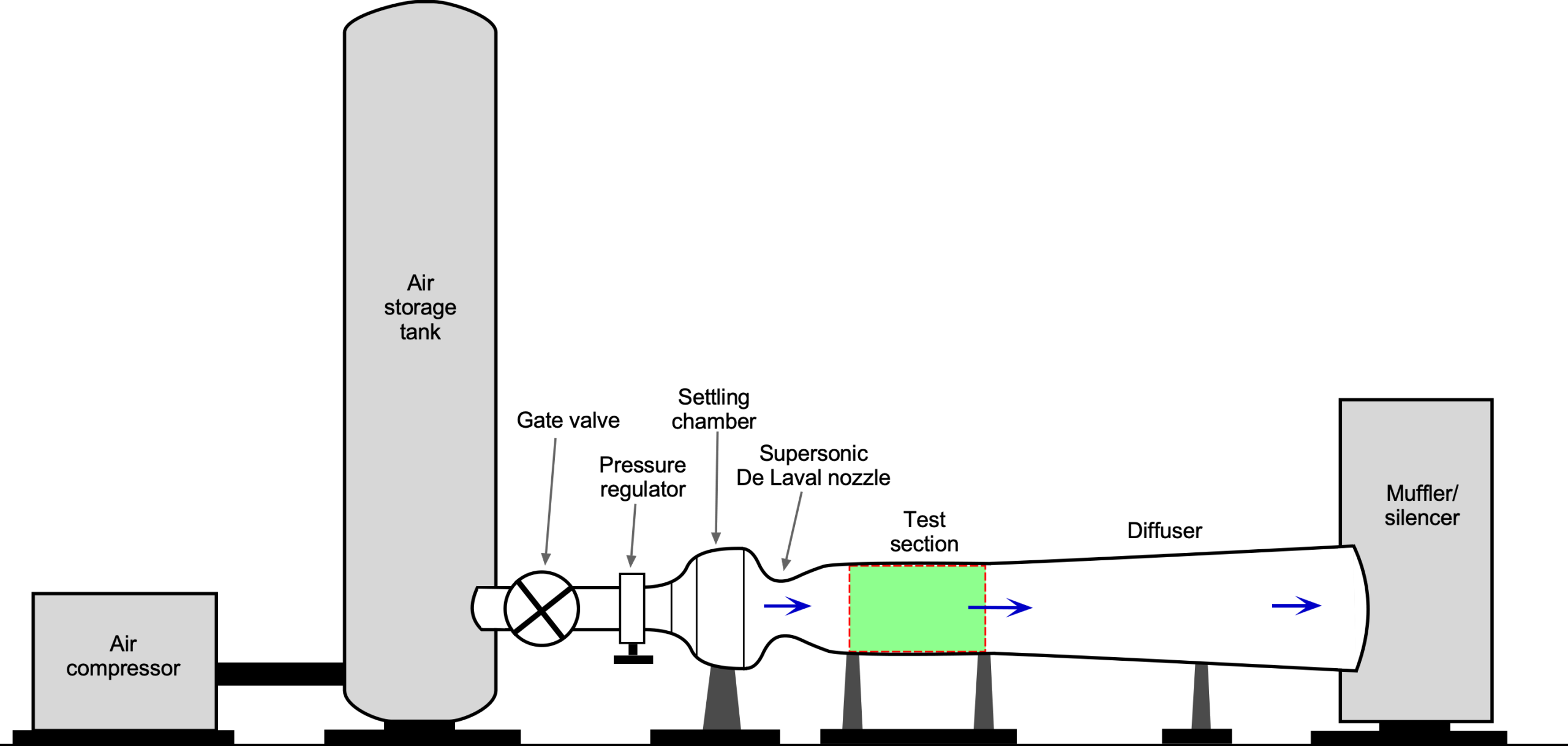
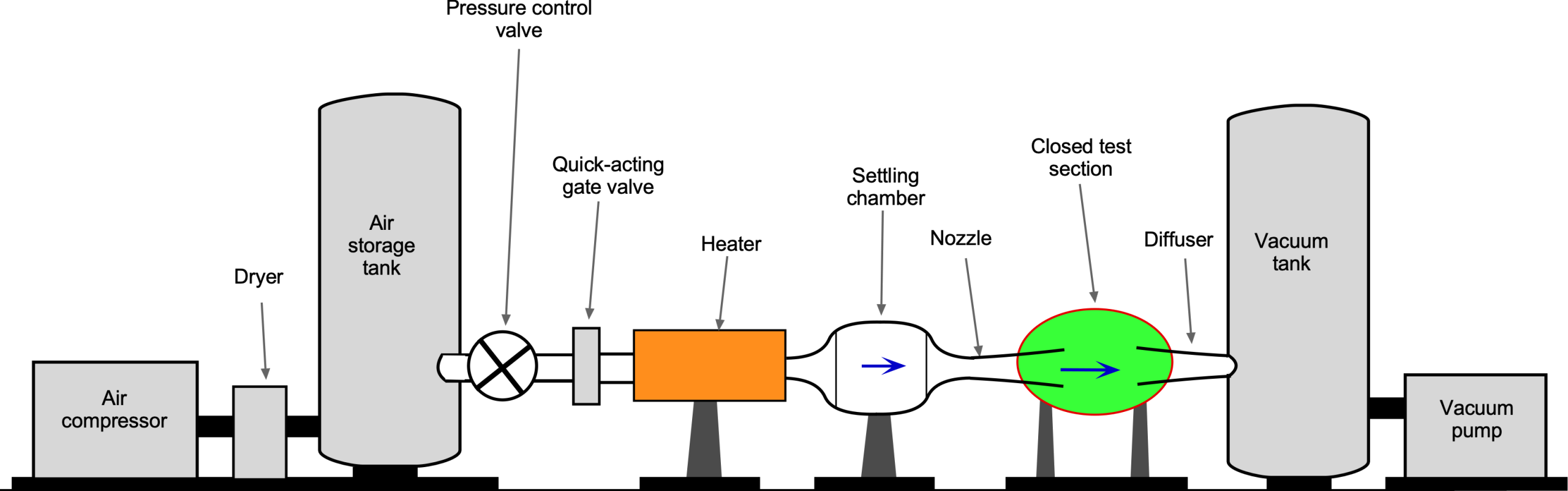
Most supersonic tunnels are of the blowdown type, which operate by releasing compressed air from high-pressure storage tanks into the circuit. The air is stored in a large reservoir at high pressure and then discharged through a precisely contoured de Laval nozzle, as shown in the figure below. The convergent section of the nozzle accelerates the flow to Mach 1 at the throat, after which the divergent section further expands it to the required supersonic Mach number in the test section. The nozzle contour is carefully designed to produce a uniform Mach number and suppress residual shock structure. Depending on the reservoir capacity and flow rate, test durations can range from a few seconds to several minutes. During these runs, the flow remains quasi-steady, allowing for accurate measurement of aerodynamic forces, pressures, and temperatures.
Upstream of the nozzle is a settling chamber or plenum, fitted with honeycomb straighteners and multiple fine screens to remove swirl and turbulence. This ensures that the flow entering the nozzle has a uniform total pressure and temperature. Because the static temperature in a supersonic expansion drops sharply, often below 100 K at Mach 4, the air must often be preheated before each run to prevent condensation, icing, or unrealistically low Reynolds numbers. Electrical heaters are commonly used, raising the stagnation temperature to about 700-900 K for Mach-4 operation.
Downstream of the test section, a supersonic diffuser decelerates the flow through a series of weak oblique shocks before returning it to subsonic speed. The diffuser then exhausts either directly to the atmosphere or, in short-duration facilities, to a low-pressure reservoir to maintain the desired pressure ratio across the nozzle. Proper diffuser design is essential to prevent flow unstart and ensure stable operation. The overall tunnel layout, therefore, consists of a high-pressure reservoir, a flow-conditioning settling chamber, a convergent-divergent nozzle, a test section, and a downstream diffuser that discharges to either the atmosphere or a vacuum, depending on the facility type.
The test section is usually rectangular and fitted with optically flat windows for schlieren or shadowgraph visualization of shock structures and expansion regions. The walls may be slightly diverging to compensate for boundary-layer growth, and pressure taps along the walls provide data for calibration of the Mach number. Models are mounted on slender sting supports or struts designed to minimize interference.
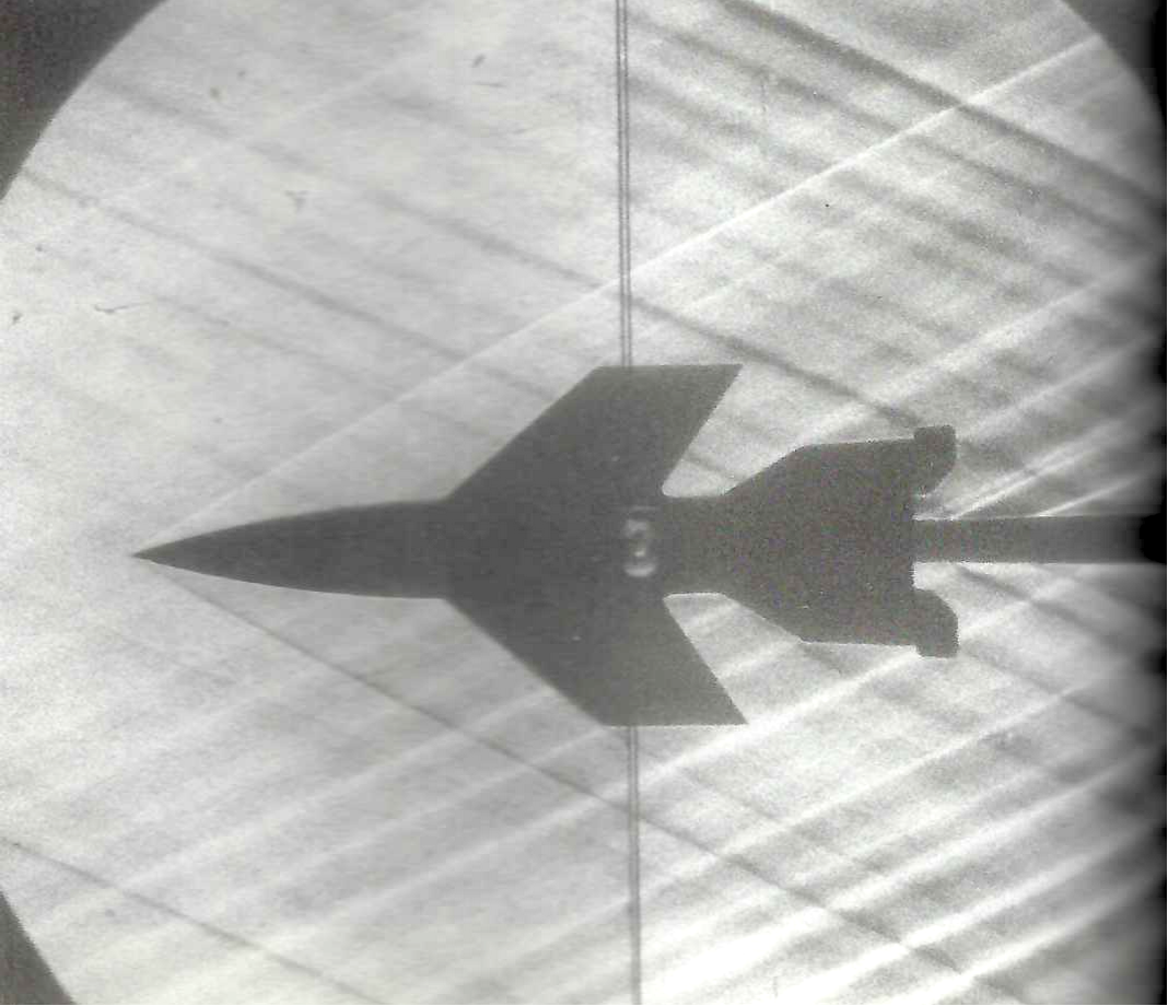
In supersonic testing, the primary focus is on understanding how high-speed flow phenomena such as shock waves, expansion fans, and shock–boundary-layer interactions affect drag, lift, stability, and control. These effects are central to the design of slender bodies, supersonic wings, and air intakes for propulsion systems. Flow visualization techniques, including schlieren and shadowgraph imaging, are widely used to observe the sharp density gradients associated with Mach waves, shock waves, and expansion regions.
Supersonic wind tunnels are essential for the development of high-speed aircraft, missiles, and propulsion systems. They provide the controlled conditions needed to study phenomena that cannot be replicated at lower Mach numbers, such as transonic-to-supersonic shock transitions, high-speed control-surface effectiveness, and inlet performance for supersonic engines. Above Mach 5, aerodynamic heating and real-gas effects become increasingly dominant, requiring even more specialized hypersonic wind-tunnel facilities to replicate these extreme conditions.
Hypersonic Wind Tunnels
Hypersonic wind tunnels, operating at Mach numbers greater than 5, are designed to reproduce the extreme aerothermal conditions encountered during atmospheric reentry and spaceflight. At these speeds, the air experiences high-temperature gas effects such as vibrational excitation, molecular dissociation, ionization, and intense boundary-layer heating. These effects must be accurately simulated to obtain meaningful aerodynamic and thermodynamic data. Hypersonic tunnels are used to investigate the combined aerodynamic and thermal environments experienced by high-speed vehicles, particularly for evaluating thermal-protection systems.
Hypersonic facilities exist in several configurations, including continuous-flow, blowdown, and impulse types such as shock tunnels and expansion tunnels, one example being shown in the schematic below. Each configuration is capable of generating the very high total pressures and enthalpies required for representative flight testing, but they differ in their operating principles, durations, and fidelity. Continuous-flow facilities can achieve relatively long test times but usually operate at reduced total enthalpy due to power limitations. In contrast, impulse facilities can reproduce accurate flight-level stagnation enthalpy for only brief periods, typically milliseconds, by releasing stored energy from a high-pressure driver section.
Shock and expansion tunnels are impulse facilities explicitly designed for hypersonic and reentry research. In a shock tunnel, a diaphragm rupture generates a strong shock wave that compresses and heats the test gas before it expands through the nozzle into the test section. An expansion tunnel adds an additional stage that further accelerates the flow, achieving even higher Mach numbers and total enthalpies representative of orbital reentry. Although the useful test duration is limited to milliseconds or, at best, a few seconds, these facilities can accurately reproduce the temperature, pressure, and chemical state of gases at reentry speeds. This capability makes them indispensable for studying high-temperature gas dynamics, validating computational fluid dynamics models, and assessing the performance of thermal-protection materials under extreme aerothermal loading.
")
Comparison of Supersonic and Hypersonic Wind Tunnels
Supersonic and hypersonic facilities share the same fundamental purpose—producing steady, well-characterized high-speed flow for aerodynamic testing. Still, they differ markedly in the physical effects that must be modeled and in the facility design required to reproduce them. The table below summarizes their principal distinctions.
| Feature | Supersonic Wind Tunnel | Hypersonic Wind Tunnel |
|---|---|---|
| Mach number range | 1.2 – 5 | > 5 (typically 5 – 15). |
| Flow regime | Fully compressible; weak shock and expansion phenomena. | High-temperature, real-gas effects (dissociation, ionization). |
| Primary objectives | Aerodynamic forces, stability and control, inlet performance. | Aerothermal heating, material response, thermal protection. |
| Typical facility types | Blowdown or continuous-flow. | Blowdown, shock, or expansion (impulse) tunnels. |
| Total temperature (T0) | Up to ~900 K. | 2,000 – 10,000 K or higher. |
| Run time | Seconds – minutes. | Milliseconds – seconds. |
| Representative applications | High-speed aircraft, supersonic intakes, missiles. | Reentry vehicles, space capsules, hypersonic cruise vehicles. |
Components of a Low-Speed Wind Tunnel
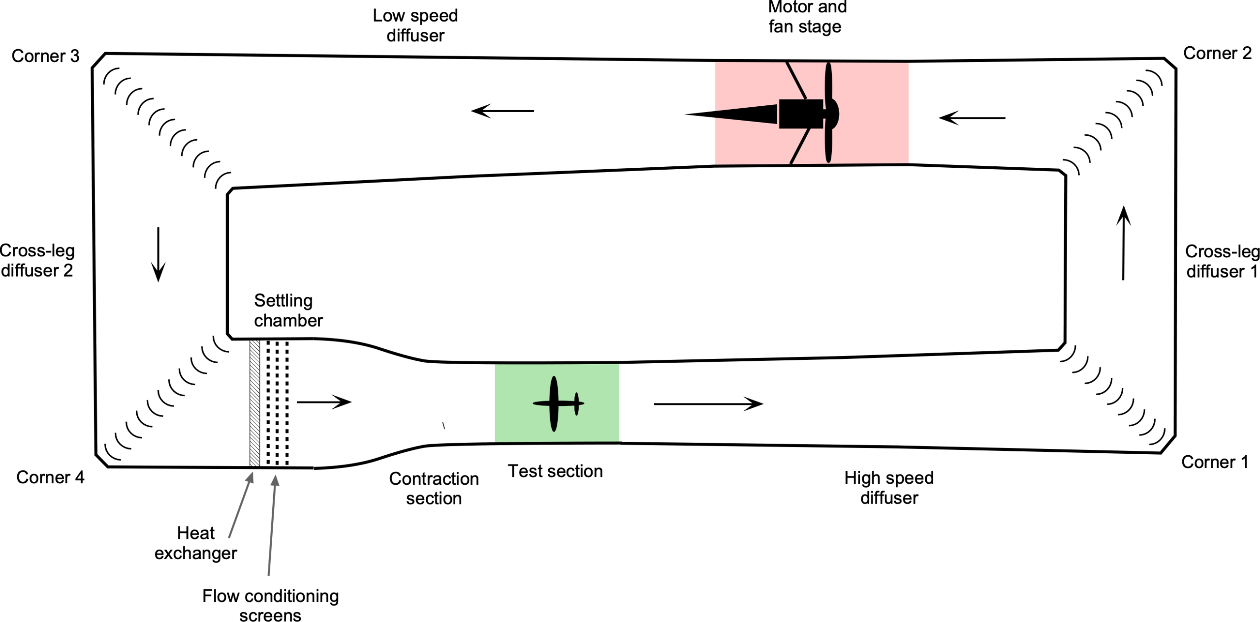
As previously discussed, there are many different types and sizes of wind tunnels. Still, it is helpful to examine in detail a relatively common low-speed, closed-return (Göttingen-type) wind tunnel. Most educational and research laboratories are equipped with one or more subsonic wind tunnels, which serve as essential tools for learning the principles and practices of aerodynamic testing. These facilities provide steady, uniform flows at moderate speeds, allowing engineers and students to study lift, drag, stability, and flow visualization under controlled and repeatable conditions.
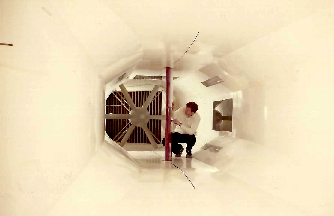
A schematic of such a low-speed wind tunnel is shown below. This particular wind tunnel has a 4 ft by 6 ft (1.22 m by 1.83 m) rectangular test section, 12 ft (3.66 m) long, with flow speeds of up to 420 ft/s (128 m/s). Additionally, the test section features approximately 65% of its surface area made of optical-grade glass, enabling flow measurements using optical diagnostic methods such as PIV.
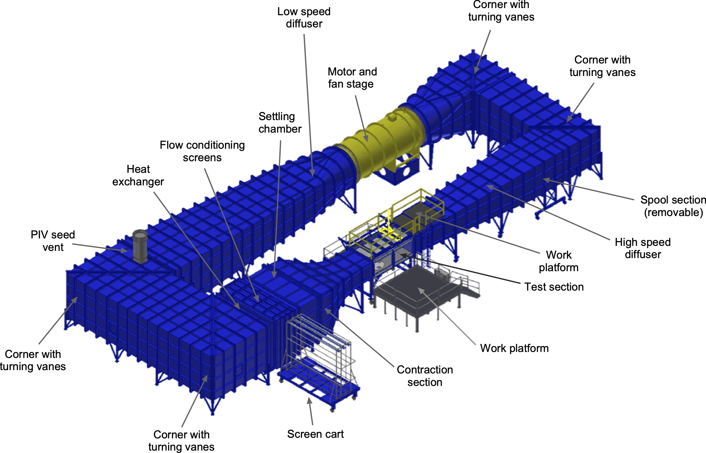
The primary components of the wind tunnel include the test section, high-speed diffuser, turning corners and cross-leg diffusers, motor and fan stage, low-speed diffuser, settling chamber, flow conditioning section, and the contraction section. Many wind tunnels are made of steel and built in shipyards, which have the necessary facilities and skilled workers to construct such large, heavy structures. Indeed, many wind tunnels look like ships turned inside out, with the frames and stringers on the outside and the smooth (flow) side on the inside.
Test Section
The test section is the most essential part of all types of wind tunnels, where the model or object under study is placed. This is the part in the tunnel circuit where the flow speed is highest; all other sections have lower velocities to minimize frictional pressure losses.
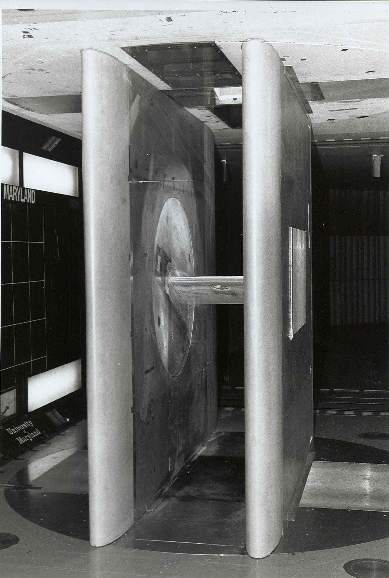
Test sections may be modular and mounted on wheels or castors, as shown in the example below, which allows different test sections to be moved in and out of the wind tunnel loop. Large doors provide easy access to the test section for installing and adjusting models and setting up instrumentation. Today, high-quality glass walls are usually used at the test section to allow access for optical measurements. At the same time, provisions for instrumentation, such as pressure taps, load cells, and high-speed cameras, can also be included. Work platforms or gantries on the sides and top of the test section may be used for access, positioning instrumentation, and designated areas for engineers to work.
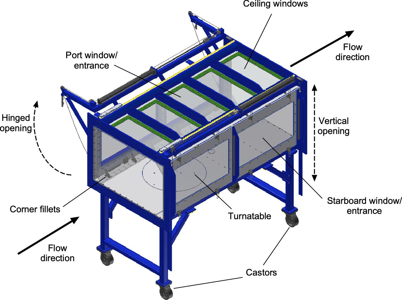
The shape of the test section is designed to minimize boundary layer effects and ensure a uniform, low-distortion flow. Corner fillets are incorporated to suppress flow separation in the corners and are tapered to zero along their length toward the downstream end. As the flow progresses downstream, viscous effects cause boundary layers to develop and grow along all four walls of the rectangular test section. This growth reduces the effective flow area, thereby accelerating the core flow velocity. To maintain uniform velocity and avoid adverse pressure gradients, the cross-sectional area of the test section is gradually increased to compensate for the boundary-layer displacement thickness. If left uncorrected, these pressure gradients can introduce horizontal buoyancy effects and distort force measurements, particularly the drag.
High-Speed Diffuser
After leaving the test section, the airflow enters the high-speed diffuser, where its velocity is gradually reduced to minimize pressure losses. This diffuser is typically long and designed with a shallow expansion angle, allowing for smooth deceleration without flow separation. To maintain attached flow, the half-angle of expansion is usually kept below about 3 , and the overall area ratio is moderate, often in the range of 1.2–1.3. A well-designed high-speed diffuser can achieve pressure recovery coefficients in the range of 0.85–0.90, i.e., losses of only 10–15%
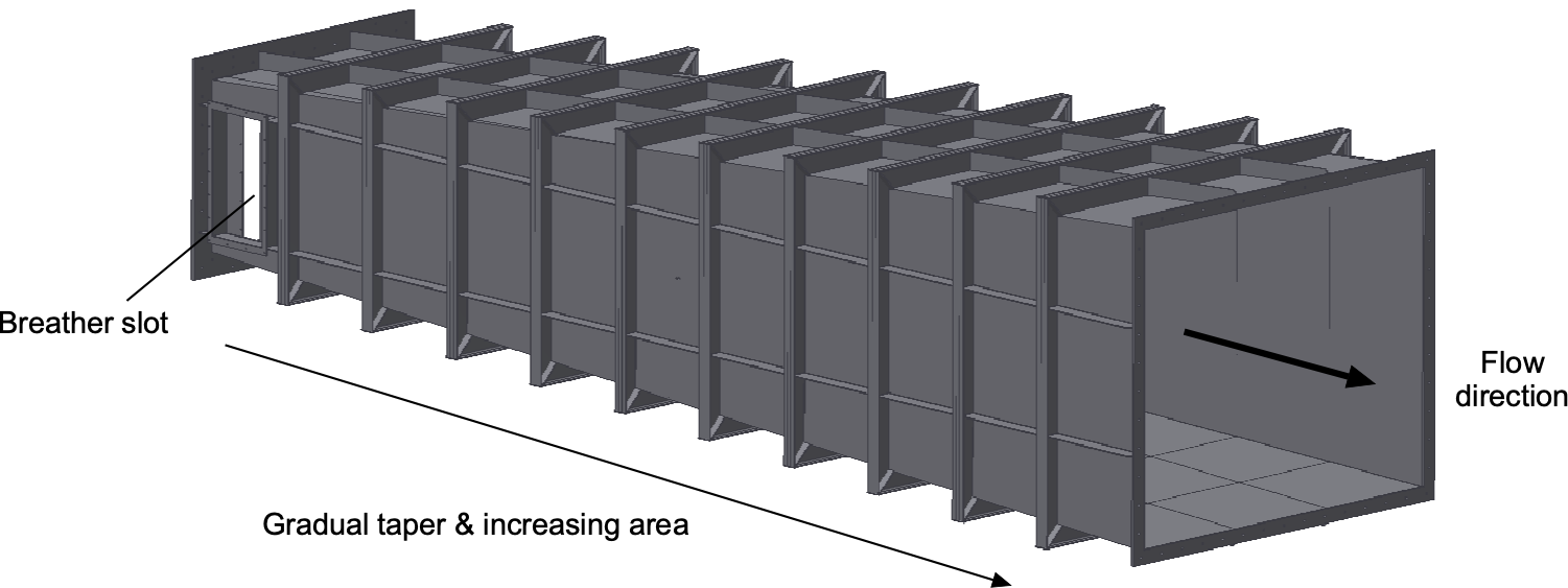
Many high-speed diffusers are fitted with breather slots along their length. These slots enable a controlled exchange of air between the test section and the surrounding atmosphere, thereby equalizing static pressure differences that can accumulate in a closed-return tunnel. The result is a steadier and more uniform flow in the test section. However, as air passes across the openings, the slots can generate considerable noise. To mitigate this effect, they are often fitted with external mufflers or baffles that direct the noise away from the test section. This approach reduces the acoustic environment at the test section. Also, it lowers turbulence levels, as pressure fluctuations and acoustic disturbances can act as sources of turbulence in the core flow.
Cross-Leg Diffusers
The purpose of the first cross-leg diffuser, spanning from corner 1 to corner 2, is to redirect the flow, further expand it, and slow it down as it approaches the fan. Each corner employs a cascade of circular-arc airfoil guide vanes with sufficient area or solidity to prevent separation and the formation of secondary vortices. These vane cascades allow the flow to turn efficiently, suppressing swirl and turbulence buildup, and help keep total-pressure losses to only a few percent per corner.
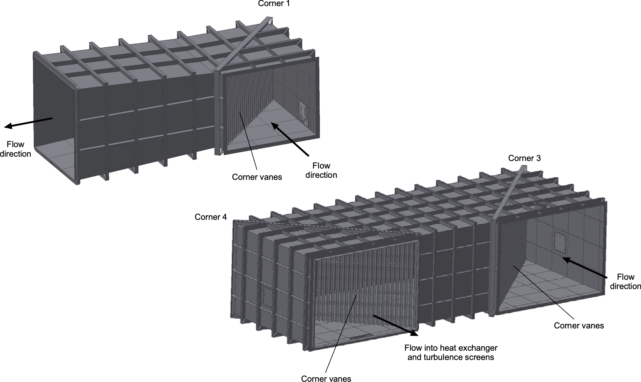
To minimize total length, this diffuser should be kept as short as practical, but the divergence angle must not be so large that the boundary layer separates from the walls. In practice, a half-angle of about 2–3 ensures a very low risk of separation in long diffusers, whereas values of 7–10 can be tolerated if the diffuser is short and the flow is well guided by turning vanes or corner fillets.
The second cross-leg diffuser extends from corner 3 to corner 4 and is generally larger in both cross-section and overall length. Because it accommodates more area growth and flow realignment, the acceptable divergence angles are governed by the same trade-offs. Longer, shallower diffusers provide more uniform flow and higher pressure recovery, while shorter, steeper diffusers reduce tunnel length but increase pressure loss and the risk of non-uniformity. Corner 4 forms the final turn before the flow enters the flow-conditioning section, where achieving a uniform velocity profile and low turbulence intensity is crucial for maintaining downstream test quality.
Corner Vanes
Airflow recirculation in a closed-circuit wind tunnel requires efficient flow turning at each corner of the return circuit. Simply curving the tunnel walls along a circular arc is insufficient because the strong curvature leads to boundary-layer thickening, flow separation, and significant energy losses. To maintain a uniform velocity distribution and prevent swirl or turbulence buildup, each corner is fitted with a cascade of turning vanes that guide the flow smoothly through the bend. The vanes may be curved plates (most common) or in the form of airfoil sections.
The performance of these vanes is characterized by their solidity, which quantifies the ratio of vane chord to spacing in the cascade and is defined as
(1) 
where  is the vane (airfoil) chord and
  is the center-to-center pitch measured normal to the local flow, as shown in the figure below.
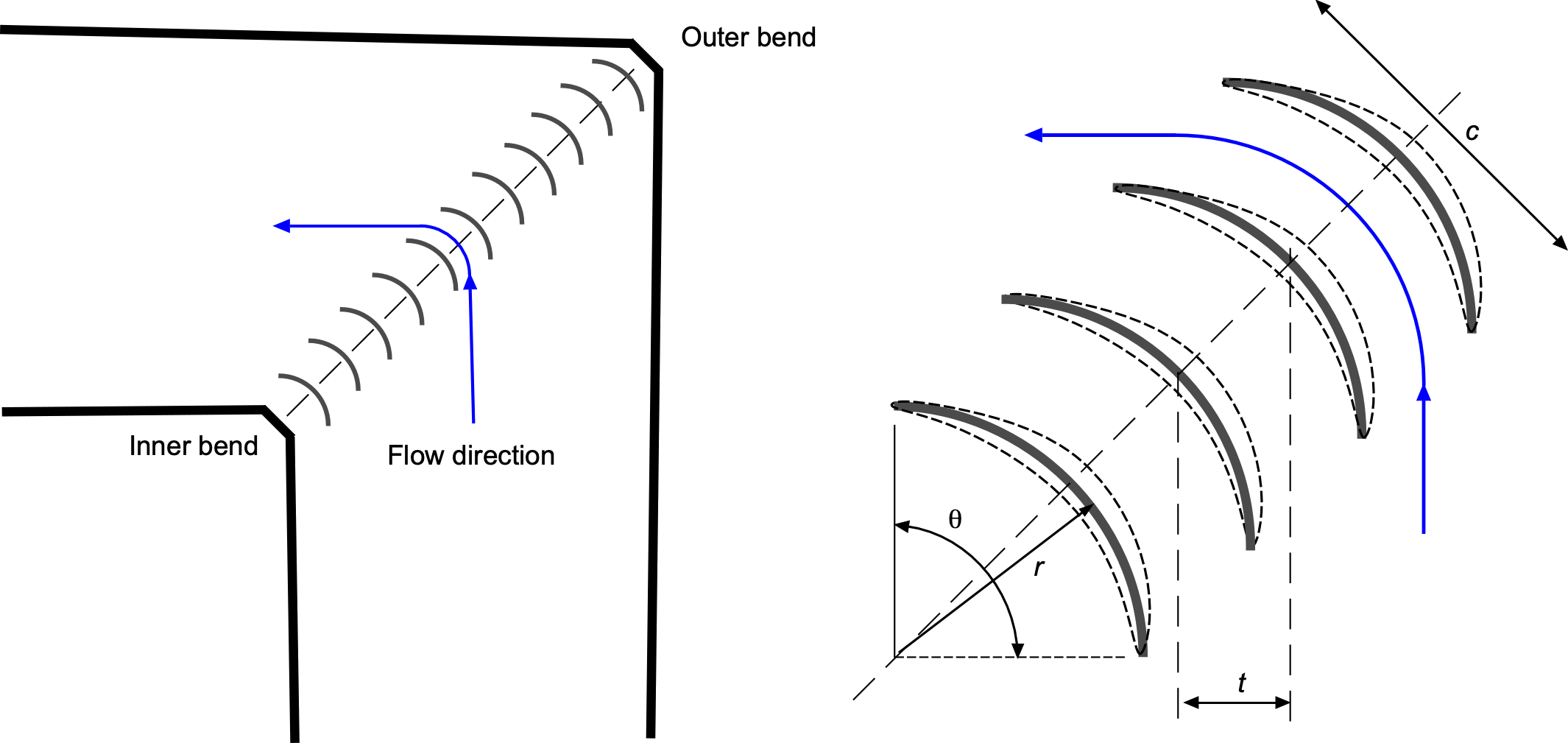
For a curved corner cascade turning through an angle  (typically
  ) with
  turning vanes, the local pitch at radius
  is
is
(2) 
giving an approximate local solidity
(3) 
Higher solidity values increase turning capability and reduce the likelihood of flow separation, but also raise blockage and pressure losses. Too low a solidity can lead to under-turning and the formation of secondary vortices. Using airfoil sections instead of simple curved plates typically reduces pressure losses by about 10–15%. Still, the extra cost of their manufacture usually does not make it worthwhile. In practice, each tunnel corner employs a cascade of circular-arc guide vanes with solidity values typically in the range of 1.0–1.5.
Motor and Fan section
The drive section houses the electric motor and fan that generate and sustain the airflow through the wind tunnel. By the time the air enters the fan, its velocity has been reduced to roughly one-tenth of the test-section speed through the action of the upstream diffusers. The fan functions as a pump, imparting energy to the flow by raising its total pressure just enough to overcome the distributed losses incurred around the tunnel circuit.
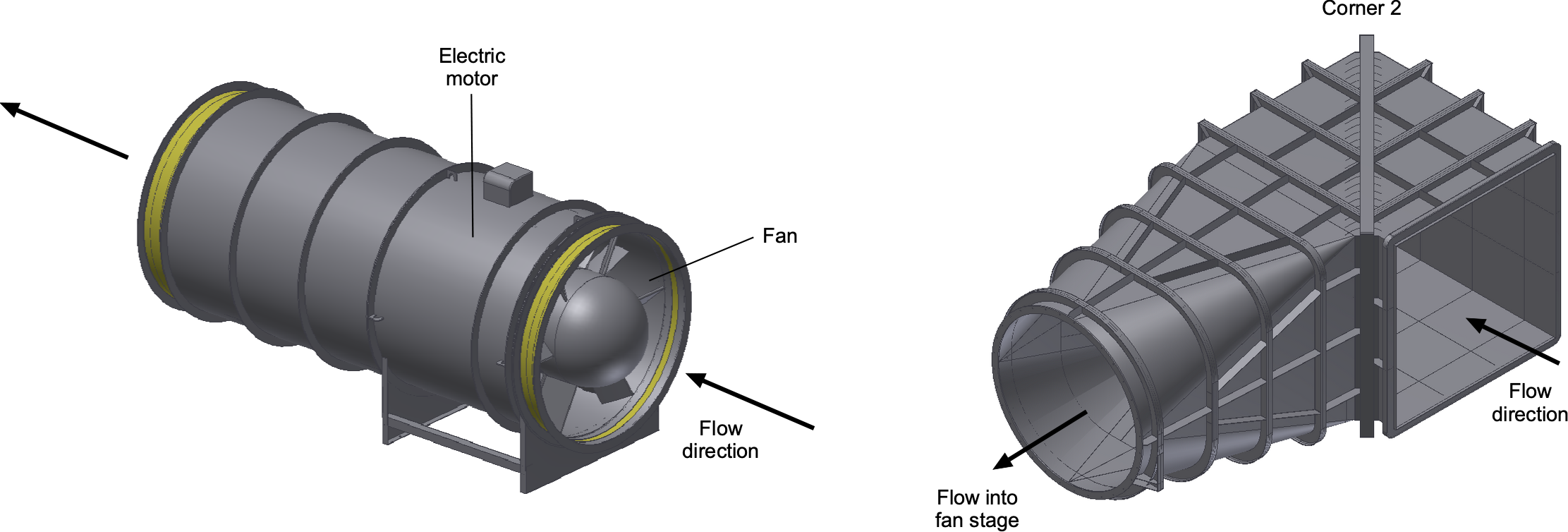
Earlier generations of wind tunnels relied on fan drives such as multi-speed motors, gearboxes, or hydraulic couplings, which could only deliver discrete speed increments. These approaches often produced coarser control of test-section velocity and higher mechanical losses. Modern wind-tunnel fans are driven by precisely controlled variable-speed motors, usually employing variable-frequency drive (VFD) systems.
The use of VFDs enables continuous adjustment of motor speed, resulting in steady, repeatable test-section velocities across the entire operating range of the tunnel. VFD-controlled motors provide smooth fan acceleration and deceleration, precise set-point control, and improved energy efficiency. This technology also reduces mechanical stresses on the drive system and allows automated test sequences in which the flow speed is ramped according to a programmed profile.
Design practice often sets the fan diameter at two to three times the test section width, ensuring sufficient mass flow handling without excessive tip speeds. In many facilities, the fan blades themselves may also have adjustable pitch, allowing the operating point to be matched to the required flow condition. Variable pitch not only improves efficiency over a wide speed range but also helps suppress instabilities such as stall or surge in the fan stage. To limit compressibility and noise, fan tip speeds are generally kept below Mach 0.7, which limits the rotational speed for a given diameter. The motor power requirement scales with the dynamic pressure in the test section and the tunnel cross-sectional area, so even modest increases in flow velocity lead to significant increases in installed drive power. In well-designed drive sections, the overall efficiency of power transfer from the motor, converted to test-section flow energy, can exceed 80%, making this component central to tunnel performance.
Low-Speed Diffuser
After the fan stage, the airflow enters the low-speed diffuser, where its velocity is reduced further to recover static pressure and minimize pressure losses. Like the high-speed diffuser, this component is relatively long and has a shallow expansion angle, enabling smooth deceleration without boundary-layer separation. Typical half-angles are limited to approximately 2–3, and overall area ratios of 1.3–1.5 are commonly achieved to ensure good pressure recovery.
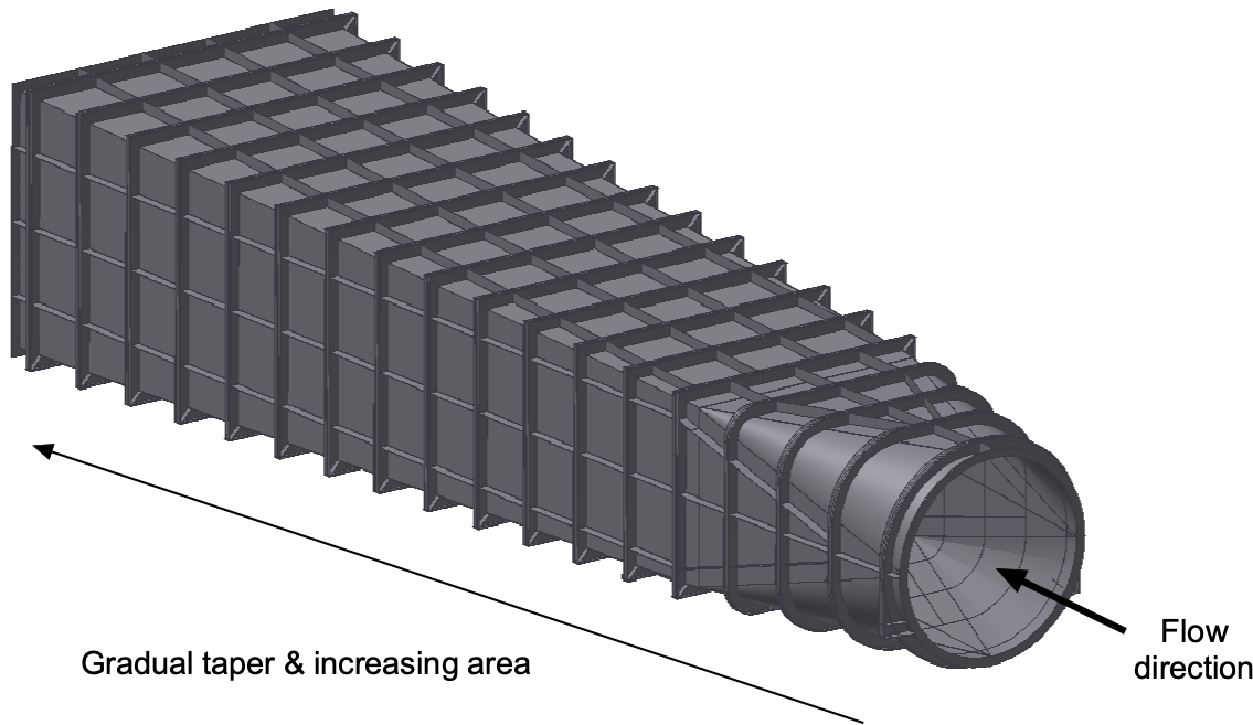
Flow Conditioning & Settling Chamber
After corner 4, the flow connects to the settling or stilling chamber. The settling or stilling chamber is located at the entrance of the test section. Its primary purpose is to precondition the air and reduce turbulence before it reaches the contraction. This goal is achieved through the use of flow straighteners, such as plates or honeycomb structures. Turbulence is then reduced using fine-mesh screens. These elements begin to remove the turbulent and angular components of the airflow, ensuring a more uniform velocity profile as it enters the contraction section. In closed-circuit wind tunnels, a heat exchanger in these regions is used to regulate the temperature of the recirculating air. The air in a closed-loop wind tunnel can become very hot from frictional losses that generate heat.
Turbulence intensity reductions can be achieved using “turbulence screens,” a staple in wind tunnel operations. These screens, also known as “anti-turbulence screens,” are made from fine wire mesh of various gauges and grid spacings, as shown in the figure below. Positioned before the contraction to the test section, they break up the larger turbulent eddies into progressively smaller ones that decay rapidly over short downstream distances. This process ensures a smoother and less turbulent flow in the test section, a prerequisite for high-quality flow measurements.
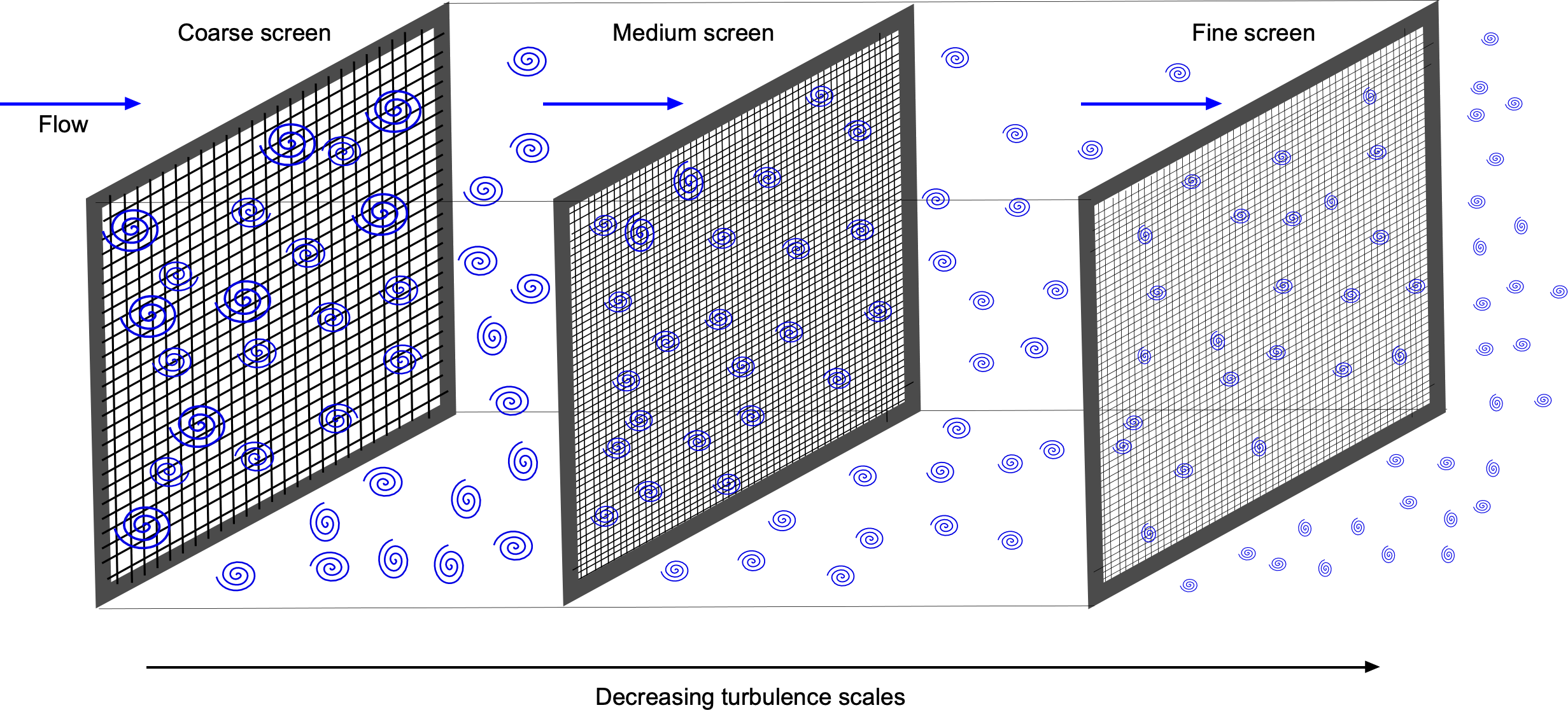
A “settling chamber” downstream of the last turbulence screen, which is usually just a short length of the constant-area, further reduces the turbulence, allowing it to reach an equilibrium state with more homogeneous turbulence levels. As the flow passes through a contraction section, the remaining turbulence is effectively squeezed out, and the flow entering the test section becomes almost laminar, although not entirely so. Turbulence levels of less than 0.1% of the freestream velocity are considered good enough to represent the flow in the higher atmosphere.
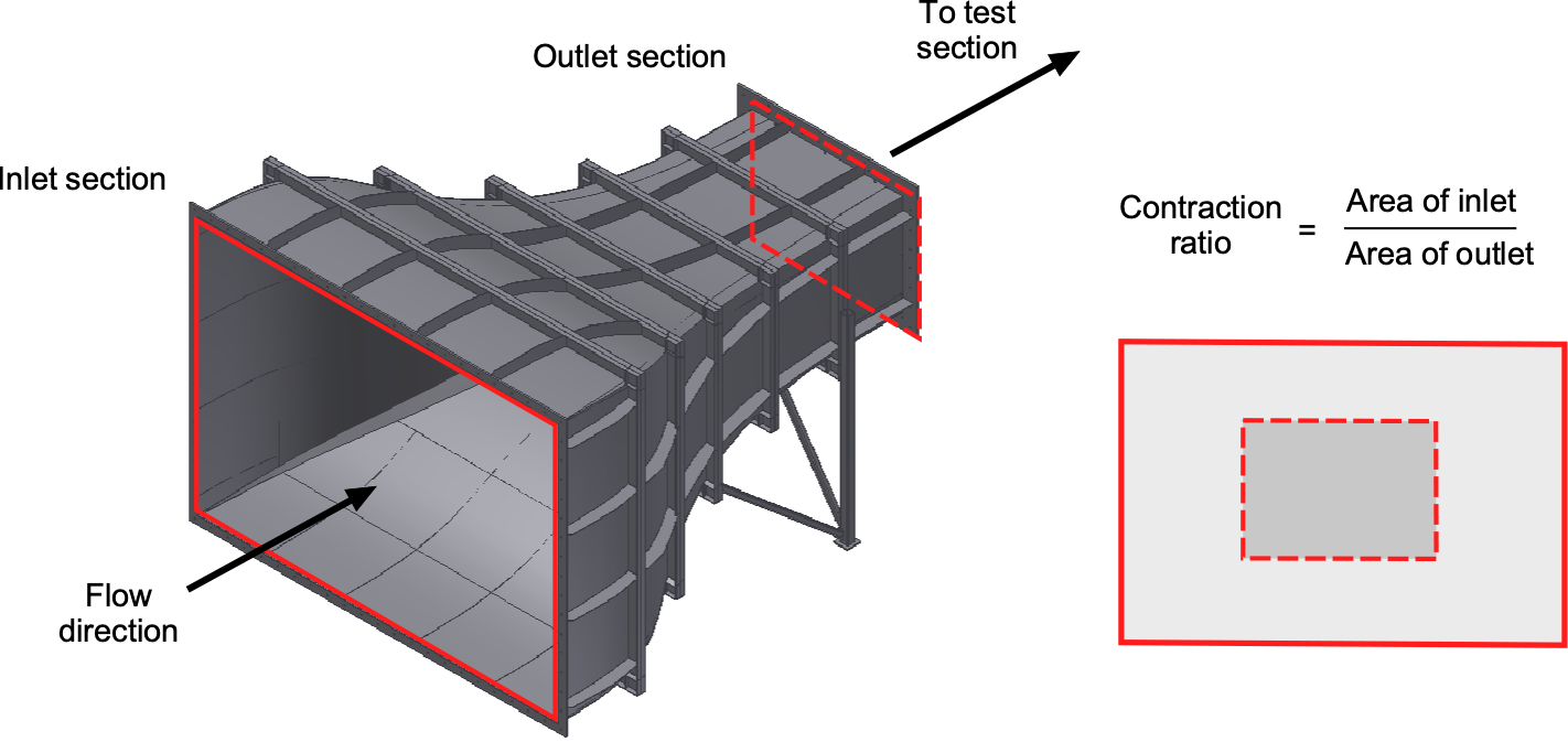
Contraction Section
The contraction section accelerates the airflow and directs it into the test section. The shape of the contraction is typically parabolic or exponential, allowing for a smooth and continuous acceleration. The ratio of the inlet area to the outlet area, known as the contraction ratio, is carefully selected based on the desired flow characteristics, and is typically about 7:1. While the purpose of the contraction is to speed up the flow before it reaches the test section, it also acts to squeeze out and “relaminarize” small turbulence eddies and further reduce turbulence levels of the flow in the test section.
Flow Quality
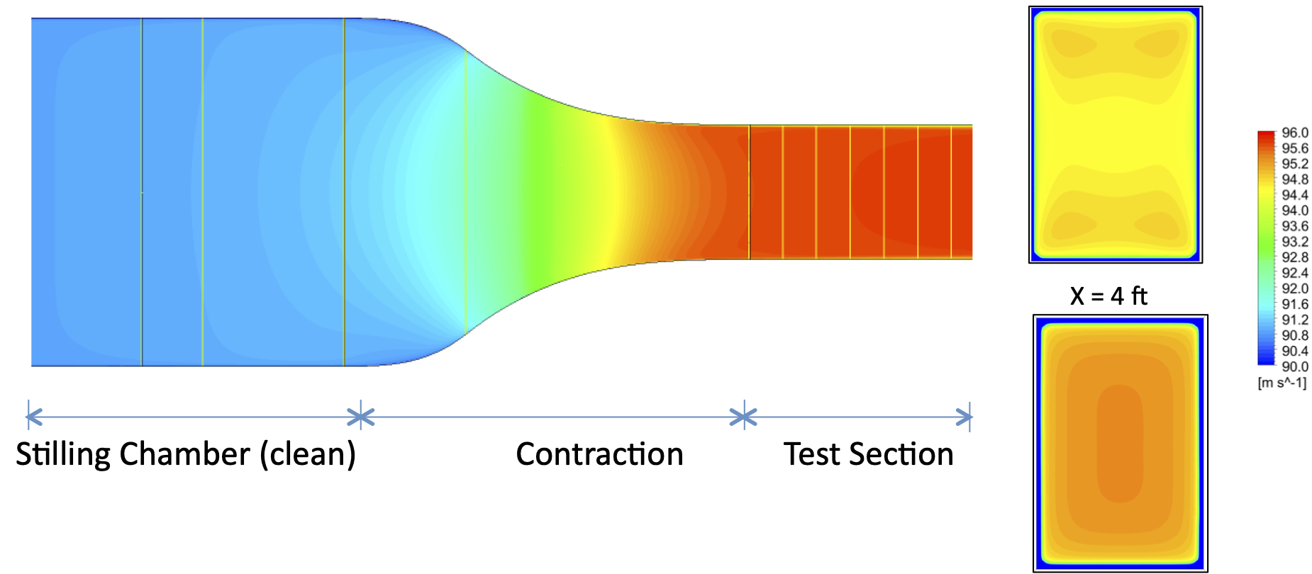
The design of a modern wind tunnel is a complex affair because it is usually customized to meet a set of unique testing requirements, including the test articles themselves and the types of measurements to be made. One of the challenges in wind tunnel design is achieving uniform flow properties in the test section, i.e., uniform velocities in both magnitude and direction, with minimal flow angularity (typically less than 0.1 degrees) throughout its entire length. This process requires close attention to the internal flow quality throughout the entire wind tunnel circuit, including the flow through the fan. Special attention must also be paid to the contraction before the test section.
Today, CFD methods are used to aid in the design of wind tunnels and can be employed to predict boundary-layer thickness and turbulence levels. The shape of the contraction can then be contoured iteratively to ensure optimal flow uniformity at the entrance to the test section and along its entire length. Appropriately shaped and tapered corner fillets, extending from the contraction and along the test section length, are also part of the design solution to account for boundary layer displacement effects.
Flow quality is one of the most critical indicators of a wind tunnel’s performance, as it sets the baseline for the accuracy and repeatability of all aerodynamic measurements. Even if balances, sensors, and reduction methods are flawless, poor flow quality will undermine the fidelity of the results. For this reason, flow quality is treated as a defining characteristic of every facility. Four primary metrics are used to assess flow quality, namely uniformity, steadiness, turbulence intensity, and flow angularity.
Uniformity
Uniformity requires the freestream velocity to remain nearly constant across the test section. In high-quality tunnels, the velocity typically varies by no more than one to two percent of the mean value across the test-section area, ensuring that lift, drag, and moment data are not biased by spanwise or chordwise velocity gradients.
Steadiness
The second metric is steadiness, which refers to the absence of low-frequency, time-varying disturbances in the mean flow. Variations in mean velocity are generally kept within  over periods of ten seconds or longer. Such steadiness is vital for capturing subtle aerodynamic effects and for ensuring repeatability across different test runs.
Turbulence Intensity
The third metric is turbulence intensity, defined as the ratio of the root-mean-square velocity fluctuations to the mean freestream speed,
(4) 
where  represents the velocity fluctuation and
  is the mean freestream velocity. High-quality low-speed tunnels maintain turbulence intensities below 0.1%, allowing fine aerodynamic increments to be resolved. This value is comparable to the level of atmospheric turbulence in the lower stratosphere.
Flow Angularity
The fourth metric is angularity, a measure of the deviation of the local flow direction from the nominal tunnel axis. Angularity is usually required to remain below  in both pitch and yaw to avoid corrupting force and moment data by effectively altering the model’s angle of attack. Careful design of diffusers, corners, and flow-conditioning screens is needed to minimize this effect.
A variety of diagnostic methods can be used to characterize and verify the quality of the flow. Basic smoke visualization can reveal gross flow non-uniformities, while hot-wire anemometry (HWA) provides quantitative measurements of turbulence intensity. Traverses with Pitot probes, usually of the 5-hole and 7-hole variety, are used to assess velocity uniformity and angularity. Advanced optical methods, such as Particle Image Velocimetry (PIV), may offer detailed, full-field diagnostics.
Ultimately, the ability of a tunnel to maintain high flow quality directly determines the reliability of the aerodynamic data it produces. Facilities with excellent steadiness, high uniformity, very low turbulence intensity, and minimal angularity enable the precise and repeatable determination of aerodynamic coefficients, such as lift, drag, and pitching moments, as well as surface pressures. This makes flow quality the foundation upon which all wind tunnel testing depends.
Test Section Shapes & Sizes
The flow quality in the test section is strongly influenced by its size and shape. Test sections are designed to provide a uniform, well-characterized flow environment, enabling aerodynamic measurements with minimal distortion. The intended application dictates the geometry, operating speed regime, and scale of the test models.
Cross-Section
The most common cross-sectional shapes are rectangular, circular, octagonal, and (less commonly) elliptical, as shown in the schematic below. Rectangular test sections are widely used in low-speed and transonic tunnels, where slotted or perforated walls can be incorporated to alleviate wall interference. Their flat walls also simplify optical access, model mounting, and the installation of interchangeable wall panels, making them exceptionally versatile. However, care is needed to manage secondary flows in the corners, which can influence boundary-layer growth and test results.
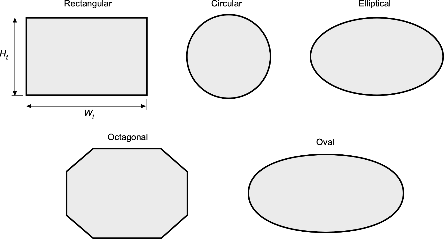
Circular test sections are commonly used in pressurized supersonic and hypersonic tunnels because their geometry efficiently resists hoop stresses and simplifies fabrication of thick-walled pressure vessels. The circular cross-section also facilitates the design of axisymmetric contoured nozzles and diffusers, allowing smooth flow expansion and minimizing corner-induced secondary flows. However, many continuous-flow and research tunnels adopt square or rectangular test sections to accommodate planar models, optical access, and instrumentation. Thus, the choice between circular and rectangular sections reflects a trade-off between structural efficiency, flow uniformity, and experimental accessibility.
Octagonal test sections are more common in low-speed tunnels. They offer a compromise between circular and rectangular designs: the multi-faceted walls approximate axisymmetry while providing flat panels that are easier to fabricate and useful for installing windows, instrumentation ports, or interchangeable wall inserts. They also tend to reduce wall interference effects when testing finite wings, compared with rectangular sections. An example is shown in the photograph below.
Elliptical test sections offer aerodynamic advantages by reducing corner-induced secondary flows and promoting more uniform boundary-layer growth. However, their higher construction cost, structural inefficiency compared to circular designs, and incompatibility with slotted or perforated wall inserts used for interference relief have limited their adoption in practice. A summary of the relative advantages of some typical wind tunnel cross-sections is given in the table below.
| Shape | Advantages | Disadvantages |
|---|---|---|
| Rectangular | Basic, low-cost construction; flat walls allow optical access, model mounting, and interchangeable panels; supports slotted or perforated walls. | Corner vortices and secondary flows can distort boundary layers. |
| Circular | Structurally efficient under pressure loading; promotes axisymmetric expansion and uniform boundary-layer growth; preferred in supersonic and hypersonic tunnels. | Less convenient for optical windows, access, or wall inserts. |
| Octagonal | Compromise between circular and rectangular; flat panels ease fabrication and allow windows or instrumentation; reduced wall interference compared to rectangular. | Less structurally efficient than circular; used mainly in low-speed tunnels, not hypersonic. |
| Elliptical | Reduces corner vortices and secondary flows; promotes more uniform boundary-layer development. | Difficult and costly to construct; structurally less efficient than circular; not compatible with slotted or perforated wall inserts. |
Special-purpose facilities may use modified cross-sections to serve specific needs. Aeroacoustic tunnels, for instance, may line the walls with acoustic treatments to absorb noise reflections. In contrast, optical test tunnels employ high-quality glass panels with anti-reflective coatings for precise imaging. Some facilities also use interchangeable wall inserts, i.e., solid, slotted, or two-dimensional inserts, so the test section can be tailored to different test programs while preserving the flow quality. The photograph below shows a two-dimensional insert placed between two false walls inside a low-speed wind tunnel. The idea is to simulate the flow over an airfoil section without using a high-aspect-ratio wing or one that spans the entire horizontal or vertical dimension of the wind tunnel.
Finally, it should be appreciated that the physical scale of the model also strongly influences the choice of test-section dimensions, together with the target Reynolds number and the allowable blockage ratio. To minimize wall interference, blockage is typically maintained below 5–10%. Low-speed research tunnels, therefore, often have larger test sections to accommodate bigger models and achieve high Reynolds numbers. In comparison, supersonic and hypersonic tunnels generally use smaller test sections to keep power requirements and total-pressure demands within practical limits.
Section Length
The length of the test section must be sufficient to provide a uniform core between the nozzle exit and the collector or first diffuser, while limiting wall boundary-layer growth. If the section is too short, the measurements encroach on the end regions where residual nozzle nonuniformity and collector-induced pressure gradients are most substantial. If it is too long, wall boundary layers thicken, and the effective area contracts, introducing an axial pressure gradient that can bias force and pressure measurements. Most closed-return facilities utilize a nearly constant-area test section or a very slight controlled divergence to offset boundary-layer displacement and maintain approximately uniform static pressure along the length.
Avoiding wake ingestion into the high-speed diffuser is critical, this phenomenon being known as wake truncation. Diffusers require a relatively uniform, low-shear inflow to achieve stable pressure recovery. When a model generates a long-separated wake, common with bluff bodies, highly loaded wings, or high-angle-of-attack stalled-flow conditions, the wake can couple with the diffuser’s adverse pressure gradient, degrade pressure recovery, and feed back into the freestream velocity in the test section as a notable unsteadiness.
Facilities that test such bluff bodies or models that produce extended wakes are often built with extended-length test sections, typically on the order of twice the largest cross-sectional dimension, and they position the model so that much of the wake intensity decays upstream of the collector. As a practical rule of thumb, when sizing and testing bluff-bodies, it is recommended to avoid issues by allowing the wake to freely develop in the test section for a distance of roughly twice the model length before the collector or diffuser entrance. It is generally not possible to make force and pressure corrections for wake truncation.
Freestream Speed Measurement
The accurate determination of freestream airspeed in the test section of a wind tunnel is fundamental for establishing consistent test conditions, normalizing aerodynamic forces, and calculating non-dimensional coefficients. To this end, flow speeds are determined using combinations of static and dynamic pressure measurements made upstream of the test section with the use of the Bernoulli equation. Probes are typically not placed in the test section because they would disturb the very clean and uniform flow that is desired to be measured. All low-speed wind tunnels are essentially large Venturis, where airflow is accelerated through the contraction section into the test section and then slowed by the diffuser section. Supersonic wind tunnels use De Laval nozzles to accelerate the flow and achieve the desired Mach number in the test section.
Static Pressure Drop Method
Consider the configuration shown below, in which the flow speed in the test section is determined by the static pressure drop across the settling chamber and the entrance to the test section. The airflow enters the mouth of area  at a flow velocity
  with pressure
  . The cross-section then contracts to a smaller area,
  , at the test section, where the velocity has increased to
  =
=  ; the velocity in the test section must increase if continuity is satisfied. The test section is vented to ambient pressure, so
  .
.
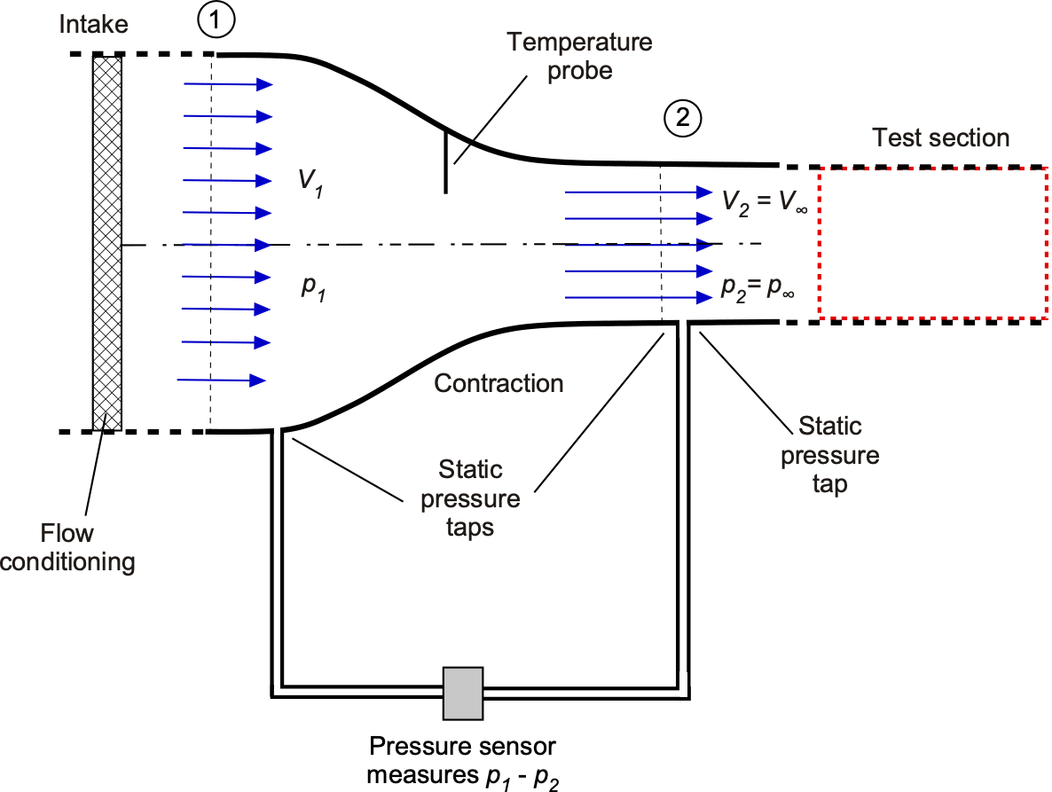
From the continuity equation, the flow velocity in the test section is
(5) 
The area ratio  is fixed for a given wind tunnel. The pressures are then related using the Bernoulli equation, i.e.,
(6) 
so that the flow velocity in the test section is
(7) 
where  is the density of the air in the test section. Air density is obtained from the ideal gas law, i.e.,
(8) 
where  is the static pressure,
  the absolute temperature, and
  the specific gas constant. In unsteady facilities such as blowdown tunnels, these parameters must be measured continuously and synchronized with force and moment data to ensure proper normalization throughout the run.
Typically, the static pressures are obtained from a pneumatic average from four taps placed around each section. This approach corrects for any small static pressure errors. However, the method is also calibrated to ensure the accuracy of the test section flow velocity. In the calibration, a reference Pitot probe is placed in the test section, and the pressure drop is measured for a range of flow speeds; any discrepancy leads to a calibration factor,  , that can be used to determine the flow speed more accurately, i.e., using
(9) 
In practice, the calibration factor for a low-speed wind tunnel is usually very close to unity.
Pitot Probe Method
Another method for measuring the flow velocity in the test section is to use a Pitot probe in the settling chamber, as illustrated in the figure below. The Pitot probe measures the total pressure,  , in the upstream section or any other convenient upstream section. This approach tends to provide a more accurate method of measuring dynamic pressure because it involves the difference between a higher and a lower pressure, rather than two lower pressures of similar magnitude. The Pitot probe is far enough upstream in a slower-moving flow that its effects downstream are negligible.
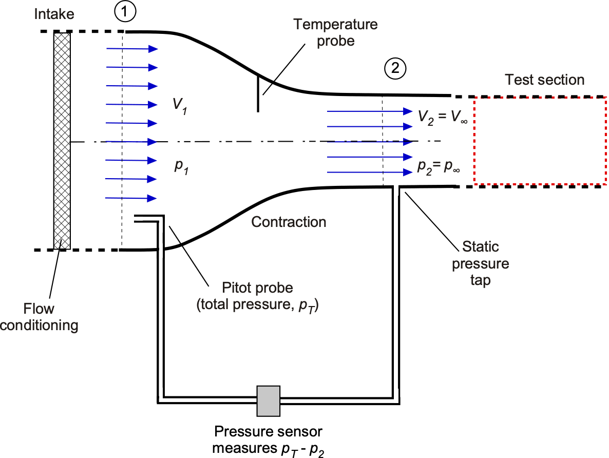
From the Bernoulli equation, then
(10) 
so that
(11) 
Again, the value of density,  , can be obtained from static pressure and temperature measurements in conjunction with the equation of state. Again, the calibration would be verified by placing a Pitot probe in the test section to obtain a calibration factor,
  , i.e.,
(12) 
where, again, will be very close to unity.
Compressible Flow Corrections
At higher Mach numbers (typically  ), compressibility effects must be considered. For an isentropic flow of a perfect gas, the Mach number
  is given by
(13) 
And the airspeed is then
(14) 
where  is the ratio of specific heats (1.4 for air), is the specific gas constant for air.
One of the most reliable methods for determining the flow speed and Mach number in a supersonic wind tunnel is the use of a Pitot probe, which measures the stagnation pressure. Combined with a measurement of the static pressure, typically taken from the wall of the test section, the Mach number can be determined using isentropic relations.
The stagnation pressure  and static pressure
  are related to the Mach number through the isentropic flow relation:
(15) 
where is the ratio of specific heats for the gas, e.g.,  for air.
Solving this equation numerically for yields the local Mach number in the test section. Once the Mach number is known, the flow speed  can be obtained from
(16) 
where  is the local speed of sound, is the specific gas constant, and
  is the static temperature of the flow.
If the stagnation temperature  is known, then the static temperature can be inferred using the isentropic relation, i.e.,
(17) 
Together, these measurements enable the complete characterization of the flow’s thermodynamic and velocity states.
Pressure Losses
One key challenge in wind tunnel design is determining the required fan or motor power to generate a desired test-section velocity or dynamic pressure. This depends on accurately estimating pressure losses throughout the tunnel circuit. Because wind tunnels contain ducts of varying shapes, areas, and transition pieces, the flow moving through them experiences friction and other losses, particularly at higher Reynolds numbers. Additional pressure losses arise from the turning vanes placed at the corners of the circuit. Typically, these are cascades of thin, airfoil-shaped plates, which help redirect flow but can introduce substantial frictional resistance. Careful estimation of these cumulative losses is essential to ensure the tunnel meets its performance targets.
In the conventional approach to wind tunnel design, the frictional losses can be estimated for the fan and initial sizing of the motor by breaking the tunnel circuit into its primary parts:
- Cylindrical sections (even if just transition pieces).
- Corners.
- Expanding sections, i.e., diffusers.
- Contracting sections, i.e., nozzles.
- Turbulence screens.
- Heat exchangers.
- Other miscellaneous parts.
In each of these sections (and there may be more than one of each), energy is lost in the form of a static pressure drop  , which can be expressed as a dimensionless local loss coefficient
(18) 
where  is the local dynamic pressure. For corners, bends, and turning vanes, the loss coefficient
  is typically based on empirical data, as previously discussed. This loss is referenced to the test section values (subscript 0) using
(19) 
Although Poiseuille’s law applies to fully developed laminar flow and is not directly applicable to the high-Reynolds-number, turbulent flows in wind tunnels, a similar scaling relationship can still be used to approximate geometric effects. Specifically, for ducts of varying cross-sections, pressure loss coefficients can be scaled based on the fourth power of the hydraulic diameter
(20) 
where  is the local hydraulic diameter of the tunnel section, and
  is the hydraulic diameter of the test section. The hydraulic diameter is defined as
(21) 
where  is the cross-sectional area and
  is the wetted perimeter of the section.
The next step is to express the energy loss per unit time,  , in terms of the test section conditions, i.e.,
(22) 
which simplifies to
(23) 
The so-called energy ratio,  , can then be defined as
(24) 
so that
(25) 
This formulation shows that minimizing  , which includes corner losses through , improves the tunnel’s efficiency and reduces the fan’s power requirement.
| Component | Typical KL Value |
|---|---|
| Straight cylindrical duct (smooth) | 0.005–0.02 |
| 90° sharp corner (no vane) | 0.3 |
| 90° smooth bend (large radius) | 0.1 |
| Turning vane cascade (airfoil shaped) | 0.05–0.15 |
| Contraction (well-designed) | 0.04–0.08 |
| Diffuser (well-designed) | 0.1–0.2 |
| Honeycomb flow straightener | 0.5–1.0 |
| Fine mesh turbulence screen | 0.2–0.5 |
The energy ratio, , represents the efficiency of a wind tunnel circuit and is inversely related to the total energy losses in the system. For a well-designed closed-return tunnel, typically ranges from 4 to 7. Lower pressure losses result in greater efficiency and reduced power demand from the fan and motor. Significant losses often arise in diffuser sections and corner vanes, making their design critical.
Calculating the loss coefficients ( ) for each section involves applying standard aerodynamic relationships for turbulent flow through ducts, fittings, vanes, turbulence screens, and other elements. Losses within the fan or motor are generally excluded from to isolate the tunnel design efficiency. Estimating these losses is necessary to determine the fan power required, called the pumping power, to achieve the target test-section velocity. Because some losses cannot be accurately estimated before construction, wind tunnel designs typically include power margins to ensure the specifications are met.
The resulting energy ratio depends on the inverse sum of the equivalent energy losses for each part of the tunnel circuit; in effect, it is the reciprocal of the losses. For a closed-return tunnel, typically ranges from 4 to 7. This outcome means that lower losses correspond to higher energy efficiency, which in turn means lower power is required to deliver air by the fan/motor. Corner vanes and diffuser sections are typically the primary sources of losses in a wind tunnel, so they must be carefully designed. Minimizing the tunnel circuit’s losses is crucial in reducing the fan’s size and the motor’s power required to drive the flow.
Determining the values of for each part of the circuit is a straightforward but often lengthy process. As previously discussed, it involves applying the fundamental aerodynamic relationships for turbulent flows through pipes and ducts. Additionally, other results are required, such as losses through the corner vanes and turbulence screens. If the losses of the motor and the fan/motor stage were included in the energy ratio, however, it would shed little light on the efficiency of the tunnel design itself. For this reason, it is usually excluded from the pressure loss calculation.
For example, consider determining the fan power required to generate a given flow velocity in the test section of a wind tunnel, an effect often referred to as the pumping power. This approach requires determining all the various pressure losses in the tunnel circuit, including frictional losses and pressure drops over the walls, turning vanes, screens, and other components. Unfortunately, not all of these effects are known, except for their estimated values, until the wind tunnel is built and tested. Therefore, the wind tunnel design may require significant power margins to fully meet the specifications.
Model Scaling & Similarity Parameters
In wind tunnel testing, models are typically smaller than the full-scale vehicle to reduce cost and facility requirements. However, to obtain meaningful results, the model must replicate the relevant flow physics of the full-scale object. This is accomplished by preserving the key non-dimensional parameters that govern the fluid dynamics of the system.
A model is said to be geometrically similar if it maintains a constant ratio for all lengths and proportions. This ensures that the shape matches the full-scale object in all three dimensions. But geometric similarity alone does not guarantee aerodynamic similarity. Dynamic similarity requires that the ratios of the forces acting in the flow are preserved. In practice, this means that certain non-dimensional parameters, most importantly the Reynolds number and Mach number, must be matched between the model and the full-scale case.
Reynolds number
The Reynolds number ( ) is the ratio of inertial to viscous forces. It governs boundary layer behavior, transition, and separation. For large-scale models or pressurized tunnels, it can be matched directly. Otherwise, corrections may be applied. Matching the Reynolds number exactly is often impractical, especially for low-speed flows in small tunnels. Instead, high-Reynolds tunnels (e.g., pressurized or cryogenic) are used, or corrections are applied based on empirical or computational fluid dynamics (CFD) data. Laminar-turbulent transition location, separation behavior, and drag prediction are susceptible to the Reynolds number.
Mach Number
The Mach number ( ) is the ratio of flow velocity to the speed of sound. It is important in compressible flows for shock formation and wave drag. In compressible flows, particularly in transonic and supersonic regimes, the concept of Mach number similarity is crucial. Unlike the Reynolds number, the Mach number is usually easier to match. Tunnels designed for compressible flows often prioritize precise control of Mach and pressure to isolate compressibility effects.
The Reynolds-Mach Conflict
In practice, it is rarely possible to match both Reynolds number and Mach number simultaneously in a wind tunnel. To see why, consider that
(26) 
Suppose a model is scaled down (reducing  ). In that case, the Reynolds number decreases unless the viscosity is lowered (e.g., through cryogenic testing) or the density is increased (e.g., by using pressurized air or a heavy gas). But increasing velocity to compensate will also raise the Mach number, possibly beyond the regime of interest. Conversely, maintaining the correct Mach number fixes the flow velocity, which may result in a Reynolds number that is far too low.
This trade-off explains why high-speed wind tunnels typically match Mach number but accept a lower Reynolds number, applying corrections or boundary-layer trips to simulate transition. In high-Reynolds tunnels (pressurized or cryogenic), conditions are set to reach flight Reynolds numbers, even if Mach similarity cannot be maintained. In subsonic low-speed tunnels, it is common to match the Reynolds number approximately (to represent boundary-layer physics) while allowing the Mach number to differ. In supersonic tunnels, Mach similarity is prioritized to represent shock-wave behavior, while Reynolds corrections are applied through analysis or empirical methods.
Froude Number
Froude number ( ) is a dimensionless parameter relevant when gravity plays a significant role in the flow field, particularly in free-surface or stratified flow simulations. While not typically a governing similarity parameter in conventional wind tunnel testing, it becomes essential in facilities used to simulate ship hydrodynamics, amphibious vehicle performance, or wave-structure interaction problems. In such contexts, proper Froude scaling ensures dynamic similarity between the model and the full-scale scenario by matching the ratio of inertial to gravitational forces.
Wall Interference
Wall interference effects are a critical concern in wind tunnel testing, particularly in narrow test sections or when testing large models. As the model occupies space within the flow, it displaces air and alters the pressure and velocity fields around it. This artificial distortion differs from the conditions encountered during free flight and must be accounted for to ensure accurate aerodynamic measurements.[5]
To reduce wall interference, some wind tunnels may employ slotted or perforated walls to allow lateral pressure relief, better simulating unbounded flow. In advanced facilities, adaptive-wall systems can adjust their contour in real time. Various correction methods are also used during data reduction, many of which have been developed empirically for each wind tunnel through calibration.
Blockage & Boundary Interference
Several primary mechanisms contribute to boundary, or wall, interference in wind tunnel testing. These arise because the solid tunnel walls constrain the flow differently than in free flight. The tunnel boundaries alter streamline curvature, restrict lateral and vertical expansion, and reflect pressure disturbances, all of which produce measurable deviations in aerodynamic forces and surface pressures on the model.
Several primary mechanisms contribute to boundary, or wall, interference in wind tunnel testing. These arise because the solid tunnel walls constrain the flow differently than in free flight. The tunnel boundaries alter streamline curvature, restrict lateral and vertical expansion, and reflect pressure disturbances, all of which produce measurable deviations in aerodynamic forces and surface pressures on the model.
The principal manifestations of wall interference are: (1) solid blockage, associated with the displacement of streamtubes around the finite thickness of the model; and (2) wake blockage, caused by the momentum deficit carried in the viscous wake of the body. In both cases, the underlying mechanism is the enforced curvature of streamlines by the tunnel walls, which alters the pressure field and feeds back on the loads measured on the model. Collectively, these boundary-induced effects are grouped under the term “wall interference,” and they must be accounted for so that wind tunnel measurements can be reduced reliably to free-air conditions.
Solid Blockage
Solid blockage is associated with the physical volume of the model, which displaces flow and reduces the available cross-sectional area of the test section. The consequence is that the streamlines can no longer develop in the same way as in free air, as shown in the figure below. A common measure of solid blockage is the blockage ratio, which is
(27) 
where  is the model’s projected frontal area and
  is the test-section area. When
  exceeds about 0.05 (5%), some solid-blockage effects can be expected.
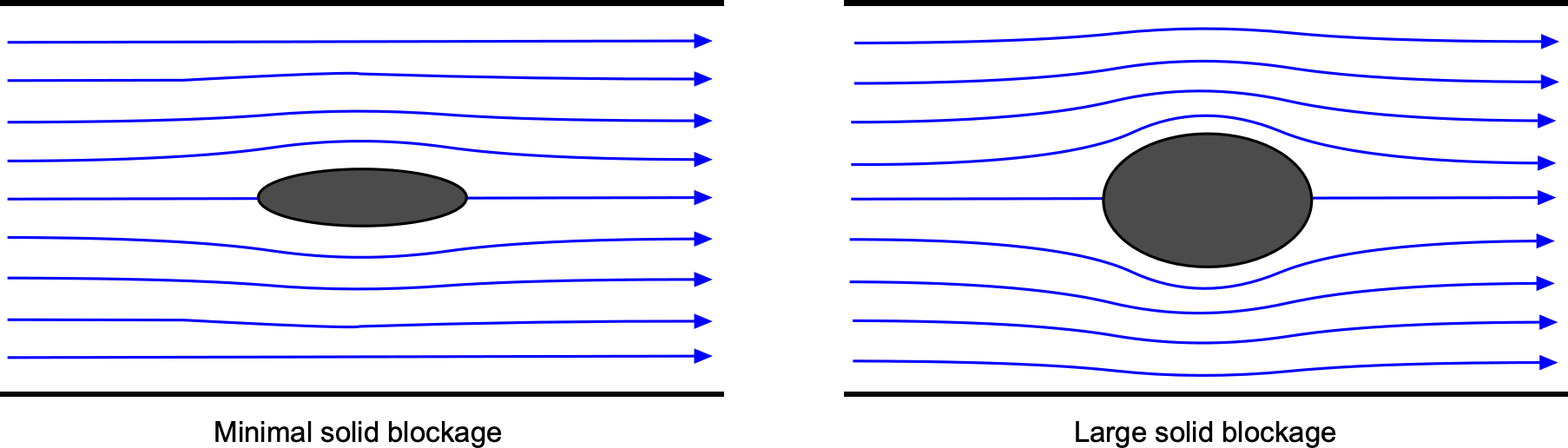
There is no closed-form theoretical prediction for the effects, so semi-empirical correlations are employed. These are often expressed as an effective freestream velocity increment of the form
(28) 
where  is an empirical factor of order unity that depends on model shape and tunnel geometry. The corrected dynamic pressure is then
(29) 
which is used to rescale aerodynamic coefficients back to their equivalent free-air values. For example, the lift coefficient may be corrected by writing
(30) 
so that the measured coefficient is reduced in proportion to the blockage ratio and an empirical calibration factor. Similar forms are often applied to other force and moment coefficients.
The practical remedies for solid blockage include either applying corrections using facility-specific calibration factors or reducing the blockage ratio by testing a smaller model. Using a smaller model, however, may introduce issues related to the Reynolds number. Practical guidelines for most wind tunnels recommend keeping blockage ratios below approximately 5%. For example, in a 3.0 m test section, a model with = 0.15 m gives = 0.05, which is acceptable.
Wake Blockage
Wake blockage occurs because the model’s viscous wake cannot naturally expand in the confined test section, as shown in the figure below. The deficit must be balanced by a streamwise pressure rise across the control volume that encloses the model and its immediate wake. Again, the consequence is that the streamlines outside the wake cannot develop as they would in free air, and the tunnel walls constrain this natural wake development.
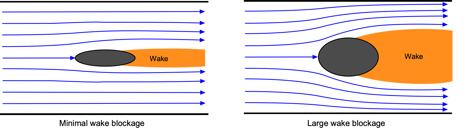
Consider steady, incompressible flow of density in a test section of area with nominal freestream speed  . Let the model have reference area and drag coefficient
  defined with respect to , so that
(31) 
where is the blockage ratio. Now the integral form of the momentum equation can be applied to a short control volume spanning the test section and enclosing the model and its nascent wake. If wall friction inside the control volume is small and the section area is nearly uniform so that the change in bulk kinetic-energy flux is small compared to the pressure forces, the streamwise momentum balance gives
(32) 
(33) 
Referencing pressures to the freestream dynamic pressure  , the associated order-of-magnitude bias in pressure coefficient is
(34) 
In practice, the pressure field distortion is not perfectly uniform. Facilities often embed the semi-empirical factor  to account for details such as wall boundary layers, nonuniform wake profiles, mild streamwise area changes, and modest compressibility, i.e.,
  , so that
(35) 
Here  denotes the pressure coefficient corrected for the nearly uniform offset induced by wake blockage. When is not yet known, then an iterative approach can be used. First, estimate from the uncorrected data, then apply Eq. 35, recompute , and repeat until convergence.
It is essential to distinguish wake blockage from solid blockage, and their effects have different corrections. Recall that solid blockage originates from inviscid acceleration and streamtube contraction around finite-thickness or bluff bodies, even in the absence of viscous drag. Wake blockage, by contrast, is tied directly to the momentum deficit produced by viscous separation and bluff-body drag. The two effects are additive in the limit of small , and comprehensive tunnel corrections typically include both, together with model-support interference and, at higher Mach numbers, mild compressibility corrections. For most streamlined models at low values of , the leading bias to  from wake blockage scales with
  as in Eq. 34. Therefore, while solid blockage can exist without much wake effect, wake blockage cannot occur without some degree of solid blockage.
Boundary (Wall) Interference
Boundary interference occurs when the flow induced by the model interacts with the solid walls of the test section, producing streamline curvature and local acceleration absent in free flight. For a finite wing or a model such as an airplane, a useful nondimensional measure is the generalized confinement ratio given by
(36) 
where  is the wing span,
  the test-section width,
  the model’s height, and
  the test-section height. Typically,
  to avoid wall interference effects.
Classical wall-interference theory models the presence of the walls using the image method, which has its origin in Glauert’s lifting line theory. The mirror systems in the lateral and vertical directions induce a modified value of the upwash at the wing, as shown in the schematic below. Using this as a basis, NACA developed methods and formulas that express the tunnel-free-air difference as a correction proportional to the model’s lift and to a geometry factor built from the confinement.[6]
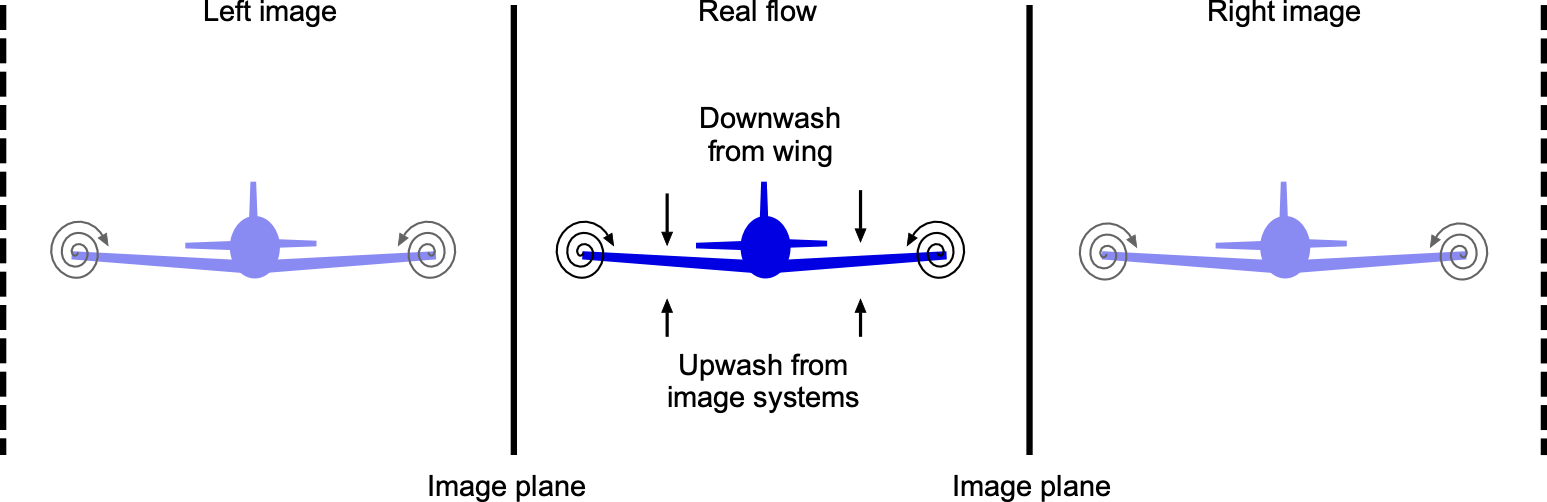
To a first order, for a model with a wing centered in the section and for small  , then
(37) 
where  and
and  , with Glauert’s compressibility factor
  . This form represents the limiting case of the more general solutions and shows directly how wall-induced upwash grows with confinement.
The induced upwash increases the effective angle of attack of the model in the tunnel, so at a fixed geometric angle, the measured lift is larger than in free air. Using the free-air slope  , then
(38) 
Equivalently, the apparent lift curve slope in the tunnel will be
(39) 
Therefore, the results can be interpreted as an apparent increase in the lift-curve slope, or, in lifting-line terms, as if the wing had a higher effective aspect ratio. A one-to-one mapping to an “effective aspect ratio” is not unique, but the interpretation highlights that wall interference alters the apparent aerodynamic efficiency.
Because the corrections scale with  and by
  , the assumption of free-air conditions deteriorates rapidly once the model gets big relative to the test section, as shown in the schematic below. Experience has established that, for typical low-speed tunnels and finite wings, keeping
  holds the interference within a few-percent envelope so that normal linear corrections are reliable.
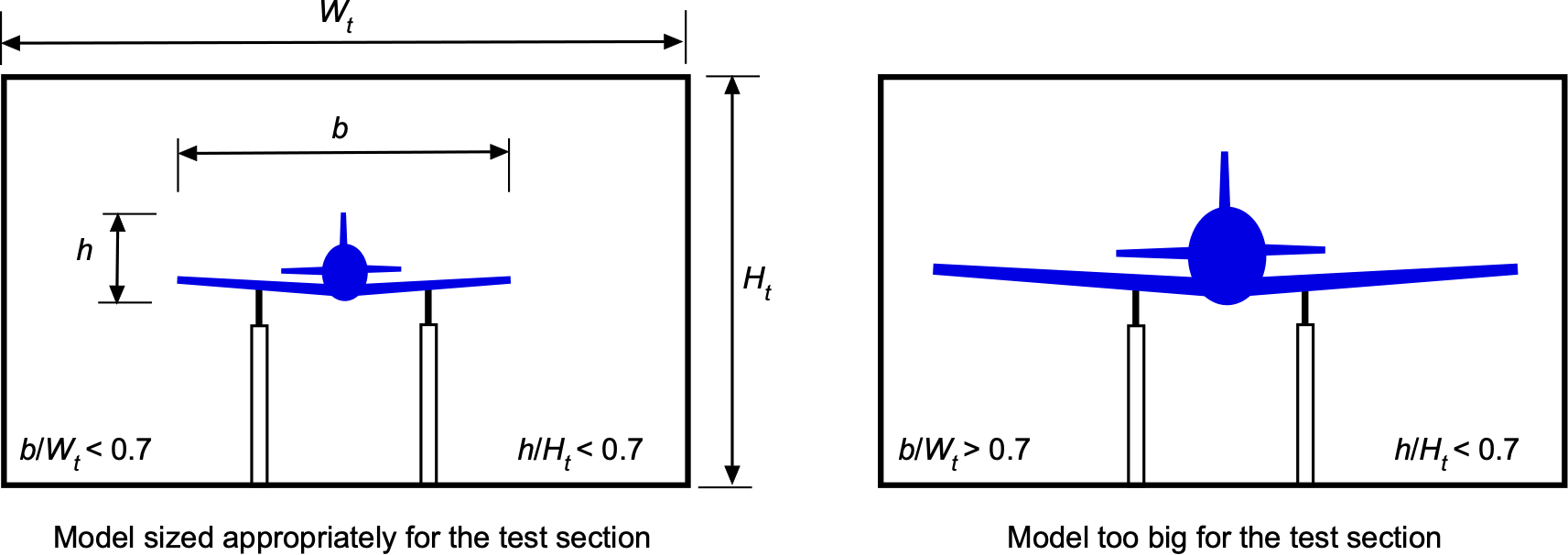
For example, if a wing has a span = 1.0 m in a = 1.5 m test section, then = 0.67, and so this is acceptable. Increasing these values further will produce noticeable wall-interference effects, and corrections will be necessary. As approaches or exceeds 0.8, the required corrections become large and increasingly nonlinear, and the basic first-order relations lose accuracy. In such regimes, the recommended remedy is to reduce confinement (e.g., a smaller model or a larger section) rather than rely on higher-order solid-wall corrections.
It should be noted that this confinement-ratio criterion applies primarily to lifting wings and surfaces. For bodies of revolution or non-lifting shapes, the more relevant measure is the blockage ratio based on frontal area, which is typically kept below about 5% of the test-section cross-sectional area to ensure acceptable free-air conditions.
Horizontal Buoyancy
Wall interference also encompasses the effects of longitudinal and vertical gradients in fluid density, pressure, or temperature in the test section, which generate buoyancy forces. The  and
and  buoyancy forces on an elemental volume
  from pressure gradients is
(40) 
Such gradients can form due to boundary-layer growth along the walls of the test section, as illustrated in the schematic below. For an axisymmetric body of length and frontal area  , the horizontal buoyancy drag increment becomes
(41) 
In most tunnels, the longitudinal pressure gradient is designed to be negligible or slightly negative, so  is positive and acts as a positive drag tare, which can be corrected for.
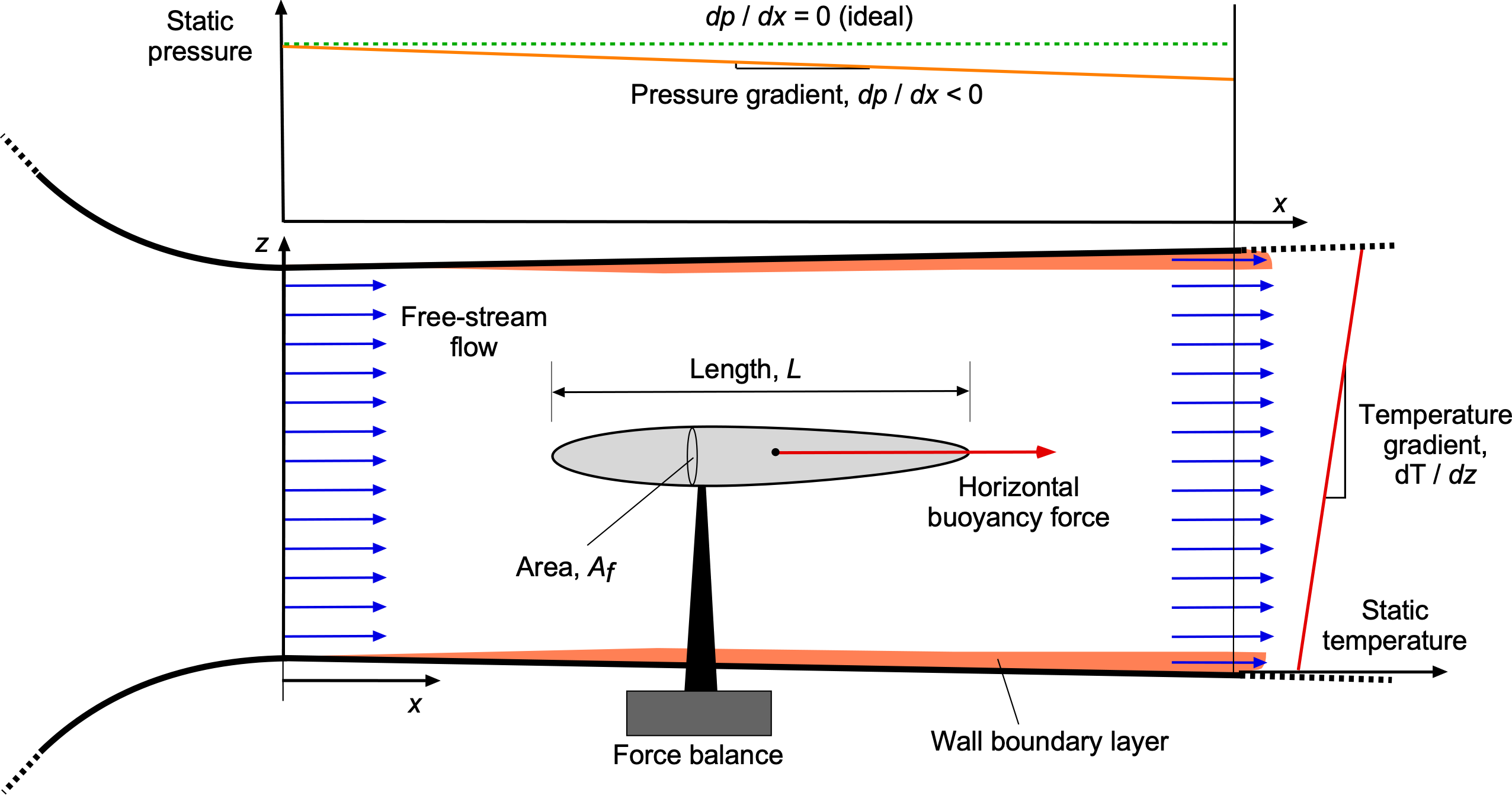
Vertical pressure gradients in wind tunnels are usually negligible. However, temperature and density gradients can also contribute to this phenomenon. For example, solar heating of the tunnel shell may introduce a vertical temperature gradient  . Using the equation of state together with the hydrostatic relation, one obtains
(42) 
and the resulting horizontal buoyancy drag tare is
(43) 
Although generally small in most wind tunnels, such taring effects can be significant in precise drag measurements.
Boundary Layer Growth
A source of wall interference related to horizontal buoyancy effects is the growth of boundary layers on the test-section walls, as shown in the schematic below. As the flow develops downstream, viscous effects reduce the effective flow area, thereby increasing the velocity of the core stream. To correct for this, the displacement thickness is introduced, i.e.,
(44) 
where  is the boundary layer thickness,
  is the local velocity, and the freestream velocity.
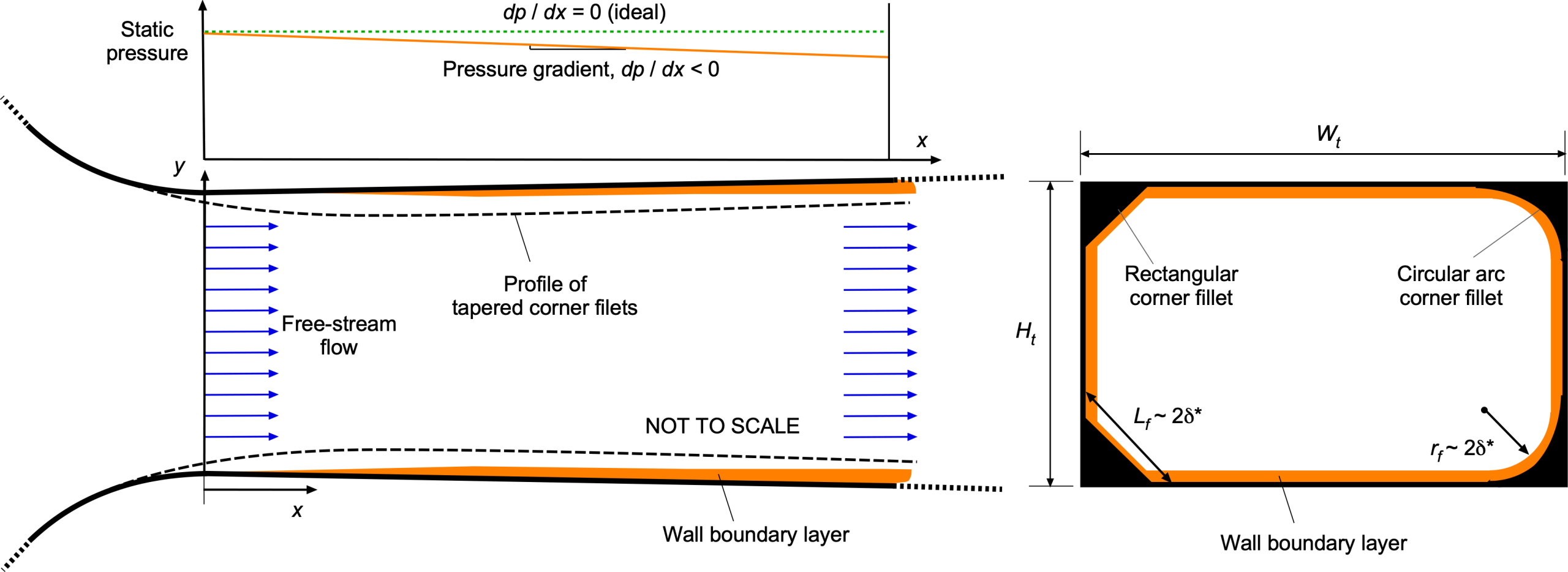
For a rectangular test section of width and height , the effective area is
(45) 
To maintain constant mass flux, the tunnel geometry must expand at a rate that offsets the displacement-blocked area, i.e.,
(46) 
Neglecting second-order terms gives
(47) 
Empirical estimates for turbulent layers include
(48) 
or, using the one-seventh power law, then
(49) 
A practical criterion for sizing the test-section corner fillets is to relate them to the boundary-layer displacement surface. The underlying principle is that the core flow behaves as if it were bounded by a virtual wall displaced inward from the physical wall by the local displacement thickness,  . At the downstream end of the test section, this offset may be expressed as
  .
.
For a circular arc fillet, the virtual flow boundary corresponds to a circle of radius  . To ensure that this virtual boundary is not smaller than that defined by the two intersecting straight walls, the following condition must be satisfied
(50) 
from which it follows that
(51) 
For a straight chamfer, providing clearance for the virtual boundary at the corner point  leads to the requirement
(52) 
Adherence to these geometric constraints promotes improved flow uniformity within the test section and minimizes the development of longitudinal pressure gradients.
Powered Models
When testing powered aircraft such as VTOL configurations, helicopter rotors, propellers, and similar installations, wall interference effects can be substantial. At low freestream velocities, the rotor/propulsor wakes and entrained secondary flows tend to recirculate within the closed test section, so “free-air” measurements are effectively impossible. At higher tunnel speeds, the wakes are convected downstream, and the flow condition generally improves. However, residual pressure gradients and swirl can still bias the data if the blockage and induced velocities are significant. Powered models also add energy to the flow, reducing the pressure jump that the fan must generate. Therefore, tracking the freestream speed becomes essential, and sufficient time is needed between test points with a powered model for the flow speed to settle.
Tests of scaled helicopter rotors are commonly performed in wind tunnels, as illustrated in the photograph below. However, because the tunnel walls confine the air, the flow through the rotor can differ significantly from that obtained in free air. The rotor imparts momentum to the surrounding air within a limited volume, accelerating the streamtube and wake through the test section, which may also impinge upon the tunnel floor. As a result, the rotor experiences a modified induced-velocity environment, which generally leads to an overestimate of both thrust and power compared to free-air operation. These confinement effects can be corrected analytically by applying suitable blockage and “ground-effect” factors to the measured data, thereby enabling reliable extrapolation to free-air conditions. In contrast, hover testing of rotors is typically conducted on an outdoor test stand or tower, where no wind-tunnel corrections are necessary.
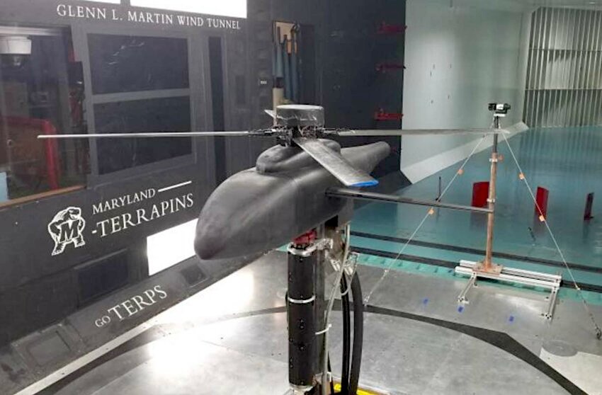
The essence of wind-tunnel corrections applied to rotor models stretches back to the work of Harry Heyson at NACA.[7] A first-order correction for wall or blockage effects for the rotor can be expressed directly in terms of the measured quantities as
(53) 
where  is the ratio of rotor-disk area to test-section area, and
  is an empirical constant that depends on the tunnel geometry. Typical values are
  for closed rectangular test sections and
  for open-jet tunnels. Here
  and
and  denote the measured thrust and power recorded by the balance, torque, or power instrumentation, i.e., before the application of any wall corrections.
A further correction must be applied for rotor wake distortion, which is a form of wake blockage. At low forward speeds, the rotor wake position is not streamwise and is skewed with respect to the freestream flow, as shown in the schematic below. The effective distance between the rotor and the floor is then based on the normal separation to the wake centerline, i.e.,  , where the wake-skew angle
  is given approximately by
(54) 
in terms of the advance ratio  and the inflow ratio
  , where
  is the hover tip speed of the rotor, which is used as a reference. The term
  represents the mean induced velocity through the rotor disk. It is related to the total flow velocity normal to the disk, which is the sum of the freestream component normal to the disk and the induced velocity. The airspeed component normal to the disk is
  , where
  is the rotor disk-tilt angle. For steady flow, the induced velocity can be obtained from the momentum (actuator-disk) relationship, i.e.,
(55) 
where  . In hover (
 ), so that the induced velocity is
(56) 
while in forward flight, a useful approximation to the induced velocity is
(57) 
Therefore, the induced velocity governs the wake skew angle and the inflow angle at the disk.
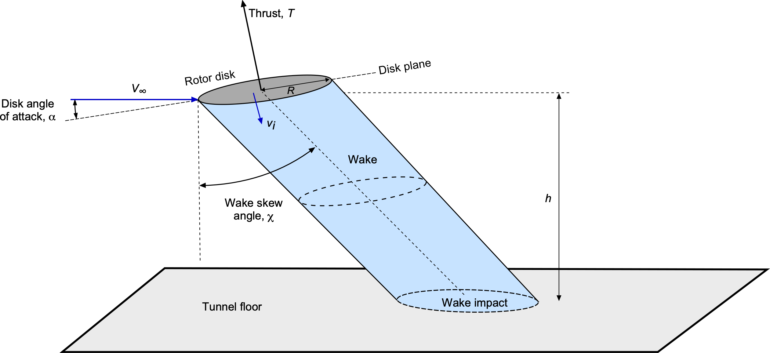
A classic correction for the ratio of the induced velocity in ground effect to that in free air is based on the method of images and can be approximated by
(58) 
which is valid for  . When the rotor is far from the floor (
 ), the ratio approaches unity and the ground effect disappears. Substituting
  into the ground-effect expression gives
(59) 
which accounts for the reduced influence of the floor as the wake becomes increasingly inclined at higher forward speeds. As the flow speed increases, the wake impinges on the tunnel floor farther downstream, and the ground-effect contribution diminishes so that  at moderate advance ratios.
Therefore, the final corrections for free-air equivalents of thrust and power are
(60) 
For typical small rotors in moderate-sized tunnels, wall corrections increase the measured thrust and power by only a few percent, while the ground-effect term becomes negligible as the forward speed increases.
In forward flight, the variation of the effective wake interference factor  diminishes, as shown in the figure below. As the freestream flow increases, the wake skews back, shifting the impingement point on the tunnel floor aft. Consequently, the ground-effect factor tends toward unity as either the height ratio
  or the wake skew angle increases. For values of
  , then corrections to the thrust and power are viable. However, a better approach is to try to avoid them altogether. For example, suppose the corrected values give
  . In that case, certain test conditions may need to be avoided, or the applied corrections to free-air conditions may be unreliable.
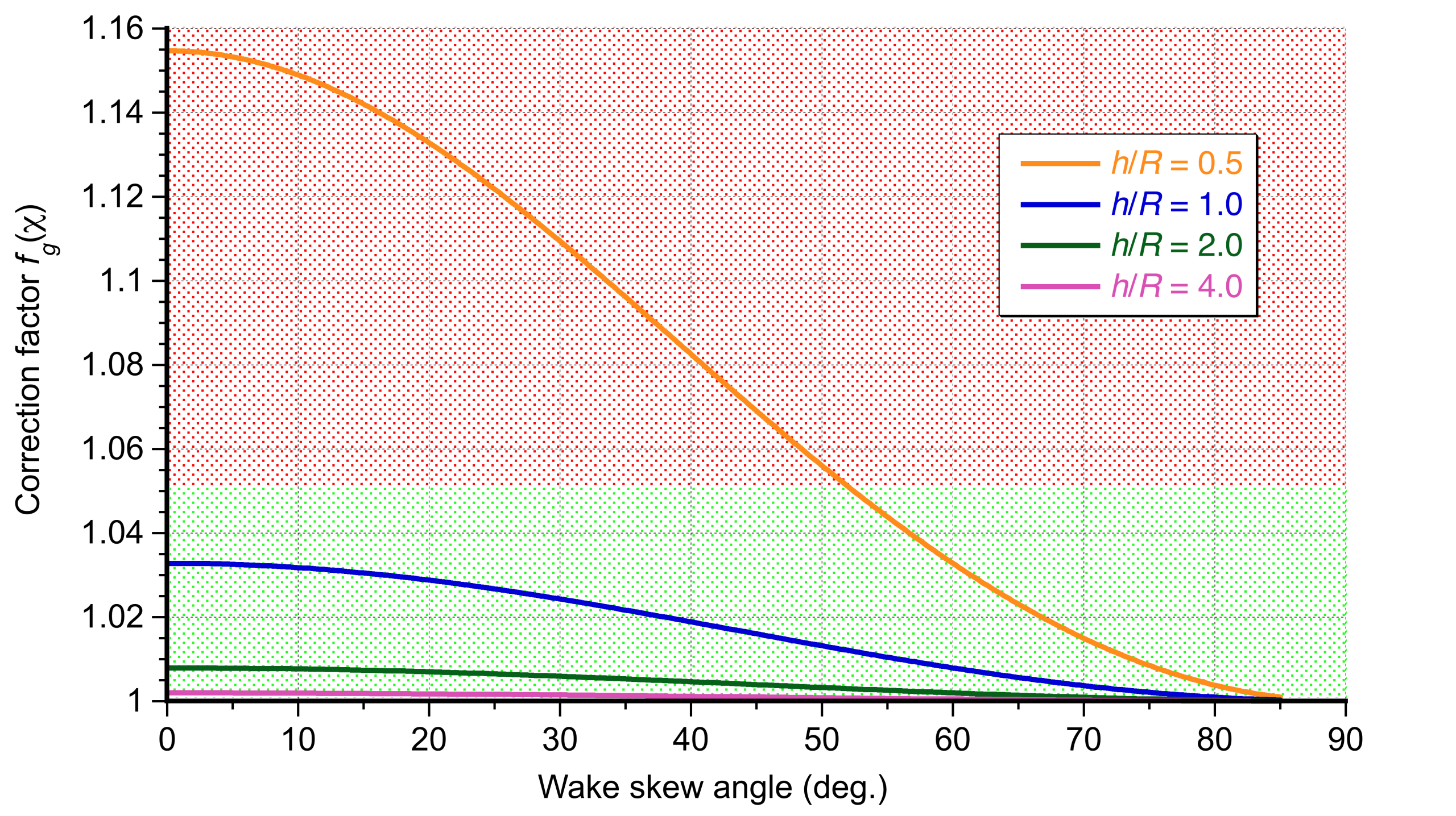 with wake skew angle for several rotor heights . For a rotor at least one radius above the floor, interference effects are minor.
If a fuselage or support body lies beneath the rotor, its projected frontal area can be included in the blockage ratio using
(61) 
where is the body’s frontal area, and  is a blockage coefficient accounting for body shape and local slipstream acceleration. It is sufficient to use
  for bodies in closed sections, and
  for streamlined bodies or bodies in open-jet tunnels. Then
  can be used in place of everywhere the wall term appears in the corrections, i.e.,
(62) 
and so
(63) 
Another way to monitor wall interference is to install static-pressure taps along the sidewalls of the test section. Comparing the measured wall pressures with the expected uniform static level provides a direct indicator of interference: a flat distribution suggests acceptable “free-air equivalent” conditions, whereas persistent departures from ambient, axial gradients, or cross-sectional asymmetries identify conditions where such equivalence cannot be achieved. In these cases, mitigation may include operating at higher test speeds, repositioning the model to increase distance from the collector, using slotted or perforated walls, adding downstream bleed, or otherwise adjusting the facility setup to isolate the floor and walls from the wake.
Instrumentation & Measurement Techniques
Modern wind tunnel testing relies on a wide range of instrumentation systems to measure aerodynamic forces, surface pressures, flow velocities, and structural deformation. The choice of instrumentation depends strongly on the test objectives, the required level of accuracy and spatial/temporal resolution, and the flow regime under investigation.
Force and moment balances provide integrated aerodynamic loads, while pressure transducers and pressure-sensitive paints resolve surface pressure distributions. Velocity fields are measured using techniques such as hot-wire anemometry (HWA), Laser Doppler Velocimetry (LDV), or Particle Image Velocimetry (PIV), each suited to different types of spatial and temporal scales. Structural deformations are monitored with strain gauges, photogrammetry, or optical marker tracking, enabling aeroelastic effects to be measured alongside aerodynamic measurements.
Balance Measurements
The use of a force balance is fundamental to wind tunnel testing because it provides the means to measure the total aerodynamic forces and moments acting on the model. These may be either internal balances, housed within the model itself, or external balances, which support the model from outside the test section. An example of this is shown in the figure below. Both internal and external balances use strain-gauge-based force transducers that are carefully calibrated to resolve the six aerodynamic components: lift, drag, side force, and the corresponding pitching, rolling, and yawing moments.
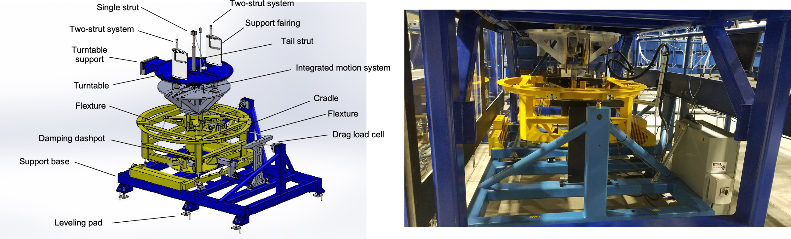
Internal balances are mounted inside the wind tunnel model, usually within the fuselage, and connect directly to the model support sting. Their primary advantage is that no external struts or linkages are exposed to the flow, thereby minimizing interference drag and preserving the model’s intended aerodynamic characteristics.
Most balances are integrated with model-positioning systems that allow the test article to be remotely pitched and yawed to a prescribed orientation with respect to the flow. In such cases, the model is connected to a vertically translating pitch strut, while yawing motion is obtained through rotation of a turntable. Some types of balances, such as a sting balance, may also allow roll. The positioning system enables the model to be automatically moved to pre-allocated test attitudes, significantly increasing the efficiency and productivity of data acquisition.
Wind tunnel balances use high-quality, temperature-compensated load cells (and sometimes pressure-compensated) to maintain calibration stability during long test runs. They are designed with sufficient stiffness to avoid resonant vibrations, yet with enough compliance to measure small force increments with high sensitivity. Modern balances can achieve accuracies of a fraction of a percent of full-scale load, making them essential for extracting reliable aerodynamic data, particularly in low-turbulence tunnels where small force increments must be resolved.
Calibration Process
Before the measurements can be made, force balances must be carefully calibrated. The calibration process involves zeroing the balance under static load conditions and applying a set of known forces and moments through lever arms and pulleys to establish the calibration matrix. An example of the process is shown in the photograph below. The balance relationship can be expressed in matrix form as
(64) 
where  is the vector of physical forces and moments,
  is the vector of measured bridge outputs, and
  is the calibration matrix. For a six-component balance, this expands to
(65) ![\begin{equation*} \begin{bmatrix} F_x \\[6pt] F_y \\[6pt] F_z \\[6pt] M_x \\[6pt] M_y \\[6pt] M_z \end{bmatrix} = \begin{bmatrix} k_{11} & k_{12} & k_{13} & k_{14} & k_{15} & k_{16} \\[6pt] k_{21} & k_{22} & k_{23} & k_{24} & k_{25} & k_{26} \\[6pt] k_{31} & k_{32} & k_{33} & k_{34} & k_{35} & k_{36} \\[6pt] k_{41} & k_{42} & k_{43} & k_{44} & k_{45} & k_{46} \\[6pt] k_{51} & k_{52} & k_{53} & k_{54} & k_{55} & k_{56} \\[6pt] k_{61} & k_{62} & k_{63} & k_{64} & k_{65} & k_{66} \end{bmatrix} \begin{bmatrix} V_1 \\[6pt] V_2 \\[6pt] V_3 \\[6pt] V_4 \\[6pt] V_5 \\[6pt] V_6 \end{bmatrix} \end{equation*}](https://eaglepubs.erau.edu/app/uploads/quicklatex/quicklatex.com-c0b1e3e7e69867fad2a9816bde66e002_l3.svg "Rendered by QuickLaTeX.com")
Here, the diagonal terms  represent the primary sensitivity of each force or moment component to its intended load. In contrast, the off-diagonal terms
  (
( ) represent the cross-sensitivities where a load in one axis induces a measurable response in another channel. The matrix is inevitably diagonally dominant.
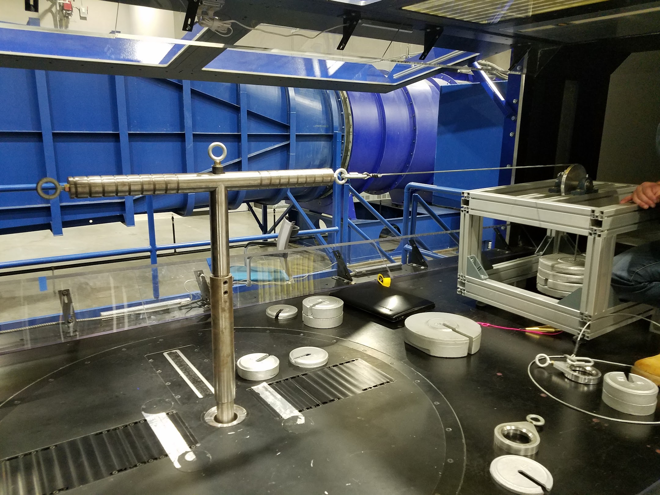
The calibration process is conducted by applying known loads using weights and pulleys, and a data acquisition system records the balance outputs . The relationship can be expressed in the matrix form as
(66) 
where  maps the forces to the voltages. The desired matrix used in testing is then obtained from the numerical inverse, i.e.,
(67) 
so that the balance outputs can be converted back into aerodynamic forces and moments. Least-squares methods are typically employed to ensure that both the main diagonal sensitivities and the off-diagonal cross-coupling terms are faithfully represented in the calibration matrix.
Mounting Configurations
Wind tunnel models can be mounted in several ways depending on the model’s size, the type of balance used, and the aerodynamic objectives of the test. The most common arrangements are the single-strut and two-strut systems, each incorporating a tail strut, as shown in the figure below. The tail strut connects to the model positioning system, so its vertical motion changes the model’s angle of attack. Strut systems are mechanically robust and can support relatively large or heavy models. Their drawback is that the exposed struts add interference drag and may disturb the local flow field, which must be accounted for during data reduction.
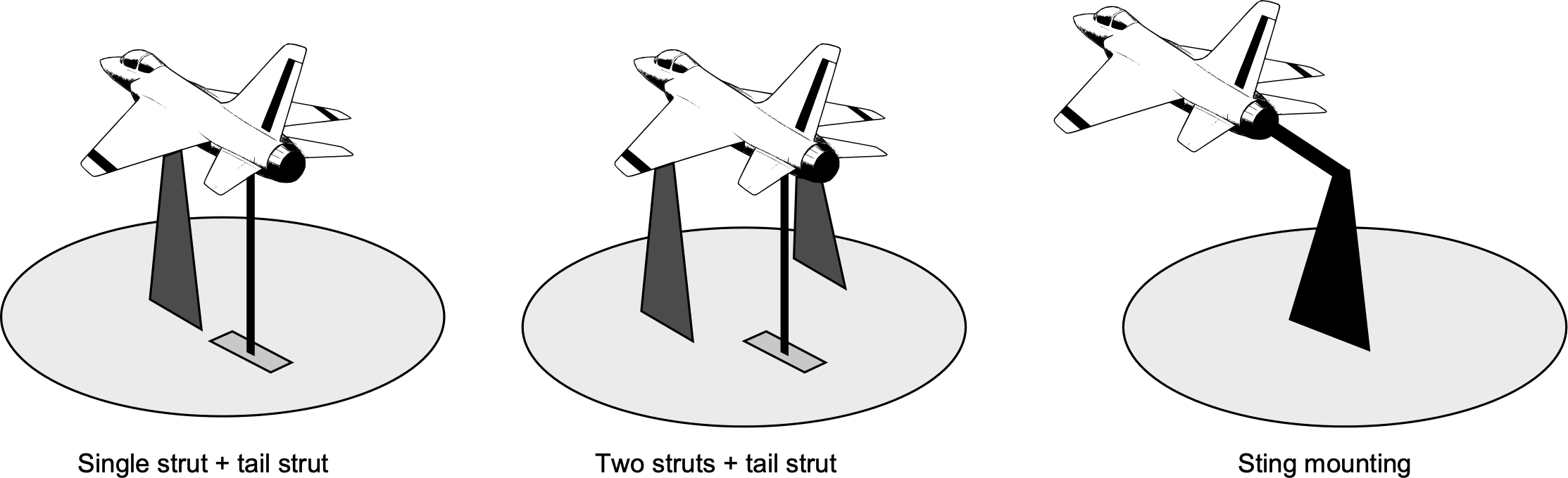
Another widely used mounting is the sting support, in which the model is carried on a cantilevered beam projecting from a vertical support. Because the sting projects behind the model, it minimizes flow interference on the wings and fuselage nose, providing cleaner aerodynamic data. Stings are often used with internal balances mounted inside the fuselage. The disadvantages are that the sting must be very stiff to resist bending and vibration, and its use is limited to models of moderate weight. Strut mounts are favored for stability and control studies or when large forces must be carried. Sting mounts are preferred for high-Mach-number testing, where minimizing support interference is critical.
The photograph below shows a wing mounted horizontally on two vertical supports. A tail strut is used to change the angle of attack, which is connected to the model positioning system. When a model in the wind tunnel is mounted on this type of support system, it becomes apparent that the supports create aerodynamic tares in the balance loads, which are always included in the measurements. The primary supports to the model are usually covered using streamlined fairings, which reduce much of the direct aerodynamic tare.
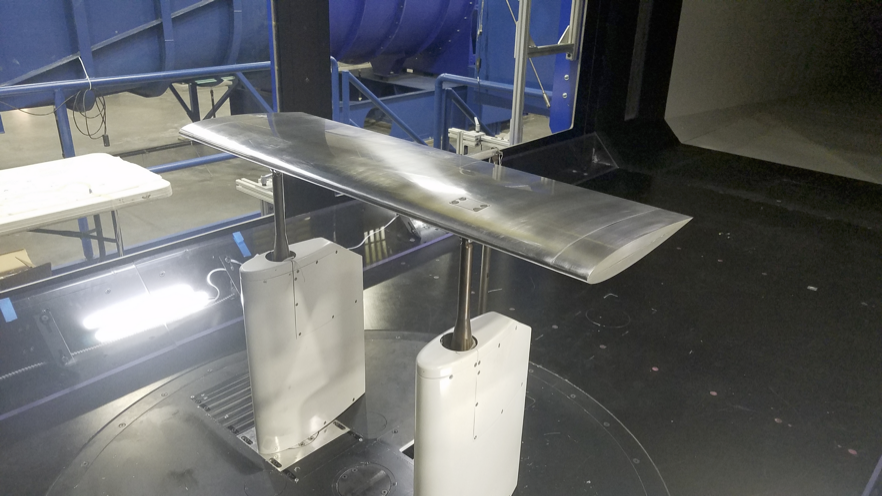
Nevertheless, a small part of the support posts is exposed to the airflow, and there is also an exposed tail pitch strut; the aerodynamic effects of these are felt on the balance. Notice that one would not want to extend the fairings all the way to the model because they would create more flow interference than the struts alone, and also limit the movement of the model on the positioning system. While typically small, these tares must still be determined by using an established process and then subtracted from the balance measurements. This approach will then provide corrected data that represent the aerodynamics of the model itself, without the effects of the supports.
Models can also be mounted vertically on the turntable, as shown in the figure below, where the angle of attack of the wing is obtained from yaw movements. While a wing is used for illustration, the model could be any other shape. To ensure that the wing is not affected by the flow along the tunnel floor, it is mounted on an offset plug with a splitter plate. This setup also mimics the other half of the wing, based on the method of images in potential flow analysis. The wing then “floats” above the splitter plate, ensuring that only the wing contributes to the balance loads. A small clearance gap is required to allow free movement, but it can be sealed with a thin application of hydraulic grease, which prevents leakage flows that would otherwise disturb the boundary layer.
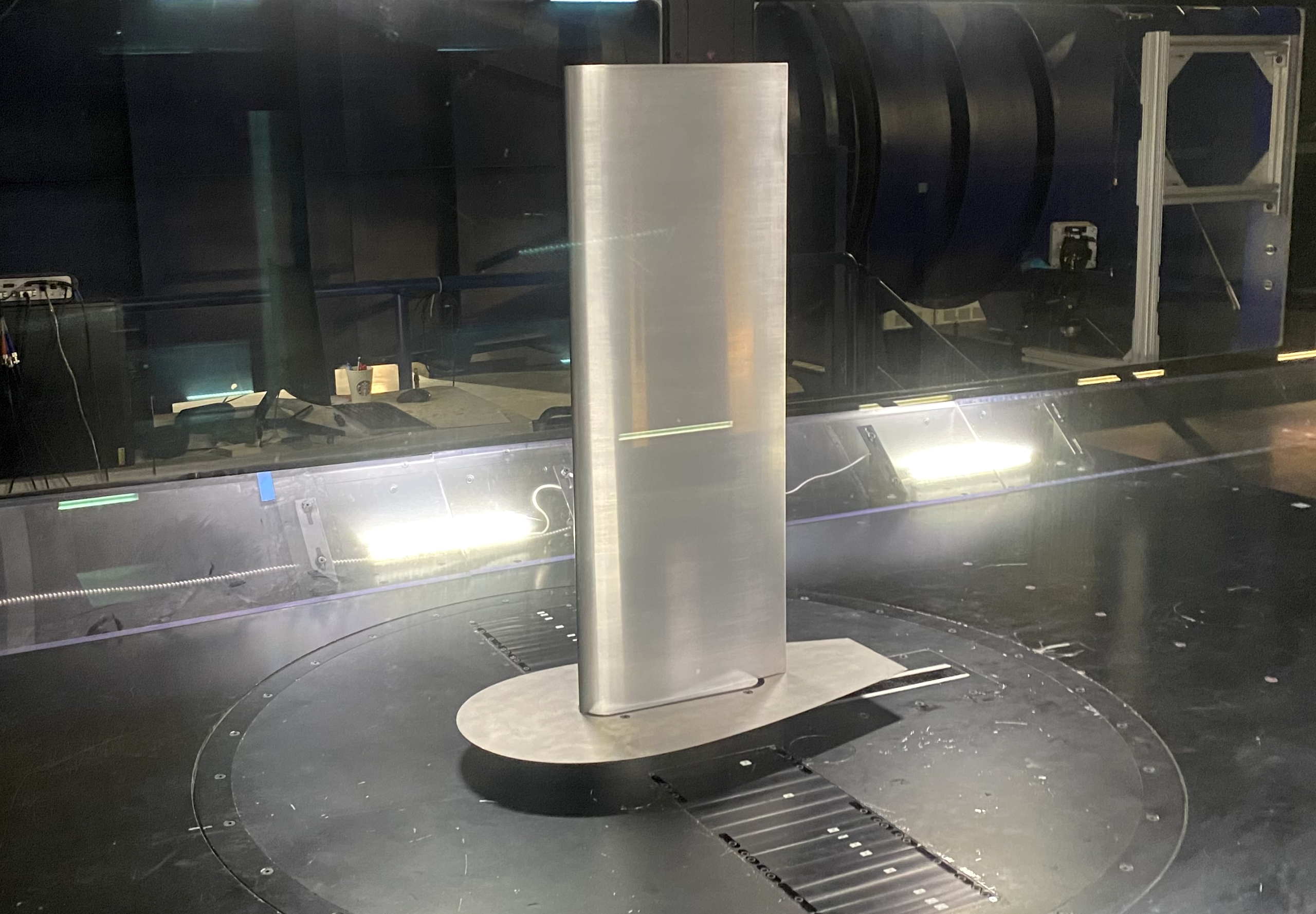
Tares
There are two types of tares: a gravity (or weight) tare and an aerodynamic tare. Accounting for the gravity tare is relatively straightforward. After the model is mounted, the balance can be re-zeroed. However, as the model moves on the positioning system, the gravity loads change, so a zero reading must be taken for each position. The gravity tares are then automatically subtracted from the loads obtained with the wind on in the data acquisition. Accounting for the aerodynamic tares, however, is a more involved process.
There are two types of aerodynamic tares: (1) a direct tare, such as the drag on the support post and the tail strut, and (2) an interference tare where the supports modify the flow about the model and the model modifies the flow about the support. Both of these effects are accounted for in wind-on measurements with an external balance and will impact all forces and moments. The significant effect is usually on drag, but for models tested at high angles to the flow, all components are typically affected.
The procedure for determining the aerodynamic tares involves three steps, as shown in the schematic below. The origins of this method are tied to the use of the “method of images” in potential flow theory, and involve creating drag to correct for drag. The first step is testing the model in a normal upright position on the support post(s), so that
(68) 
where  is representative of one of the force (or moment) values. The value of
  is what is needed, i.e., the aerodynamic effects produced on the model alone without the effects of the supports. But the aerodynamic tare
  of the lower (L) supports adds to this value. Hence, the balance measures the total force
  with both the aerodynamics on the model and the tares of the supports included together.
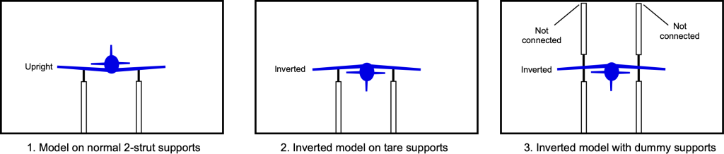
In the second step, the model is inverted on the support post(s), and all of the same tests are repeated. Mountings must therefore be installed on both the upper and lower surfaces of the model. Only in exceptional cases where the aerodynamic tares are already known from a prior calibration, or where reliable symmetry assumptions can be made, can this step be omitted. Now a second set of measurements is obtained, i.e.,
(69) 
where  is the balance value obtained from the model in the inverted position. The aerodynamic tare
  is from the effects of the supports that now have their effects on the upper (U) side of the model.
In the third step, the model is tested in the inverted position, with a dummy “image” support post, wind fairing, and pitch-rod system installed. With this configuration, the dummy “image” post is connected to the model but not to the ceiling plate, which mimics the additional aerodynamic effects of the lower (L) supports on the model when it is in the normal upright position. In this case, the measurement is
(70) 
where now an increment term appears from the aerodynamic effects of the image supports on the lower (normal) side of the model.
From the three sets of measurements ,  , and
, and  for each of the pitch (and possibly yaw) angles when the model is mounted on the balance in both the normal and inverted conditions, subtracting from gives
(71) 
So what is left is a measurement of the effects of the lower supports, . Then, returning to the measurements made at Step 1, substitute Eq. 71 into Eq. 68 to calculate , i.e.,
(72) 
which is the aerodynamic force on the model alone.
The incremental aerodynamic tare obtained in this manner then quantifies the interference effect, which is subsequently subtracted from the balance loads. The aerodynamic tares also depend on the wind speed, so unlike the gravity tares, which are removed simply by re-zeroing the balance readings, there is a different aerodynamic tare file for each wind speed. These tare data are typically used as a post-processing step to create corrected data that represent only the model’s aerodynamics, without the aerodynamic effects of the supports. While various assumptions underlie this method, including the principle of superposition, it appears to work well for wings and other models at low angles of attack when compared with measurements obtained using a sting balance.
Pressure Measurements
Surface pressures are traditionally measured using arrays of small pressure taps drilled into the model surface and plugged with a hypodermic tube. These taps are typically arranged along chordwise and spanwise lines, as shown in the figure below, allowing for the reconstruction of pressure distributions over the wing, tail, or fuselage. The taps must be as small as possible to avoid interfering with the boundary layer and may be staggered so that no one tap is immediately behind another.
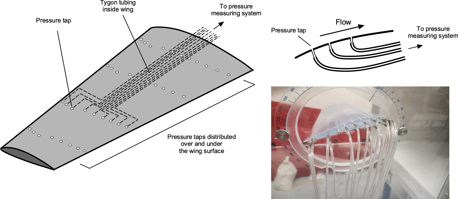
Each tap is then connected via fine Tygon tubing to an electronic pressure transducer or pressure scanner (see the photograph below), which converts the pressure into a digital signal for acquisition and processing. Modern electronic scanning systems can handle tens or hundreds of pressure taps simultaneously, enabling rapid, automated mapping of pressure fields. The modules include signal conditioning and analog-to-digital conversion, so they must be connected to a computer via an Ethernet cable.
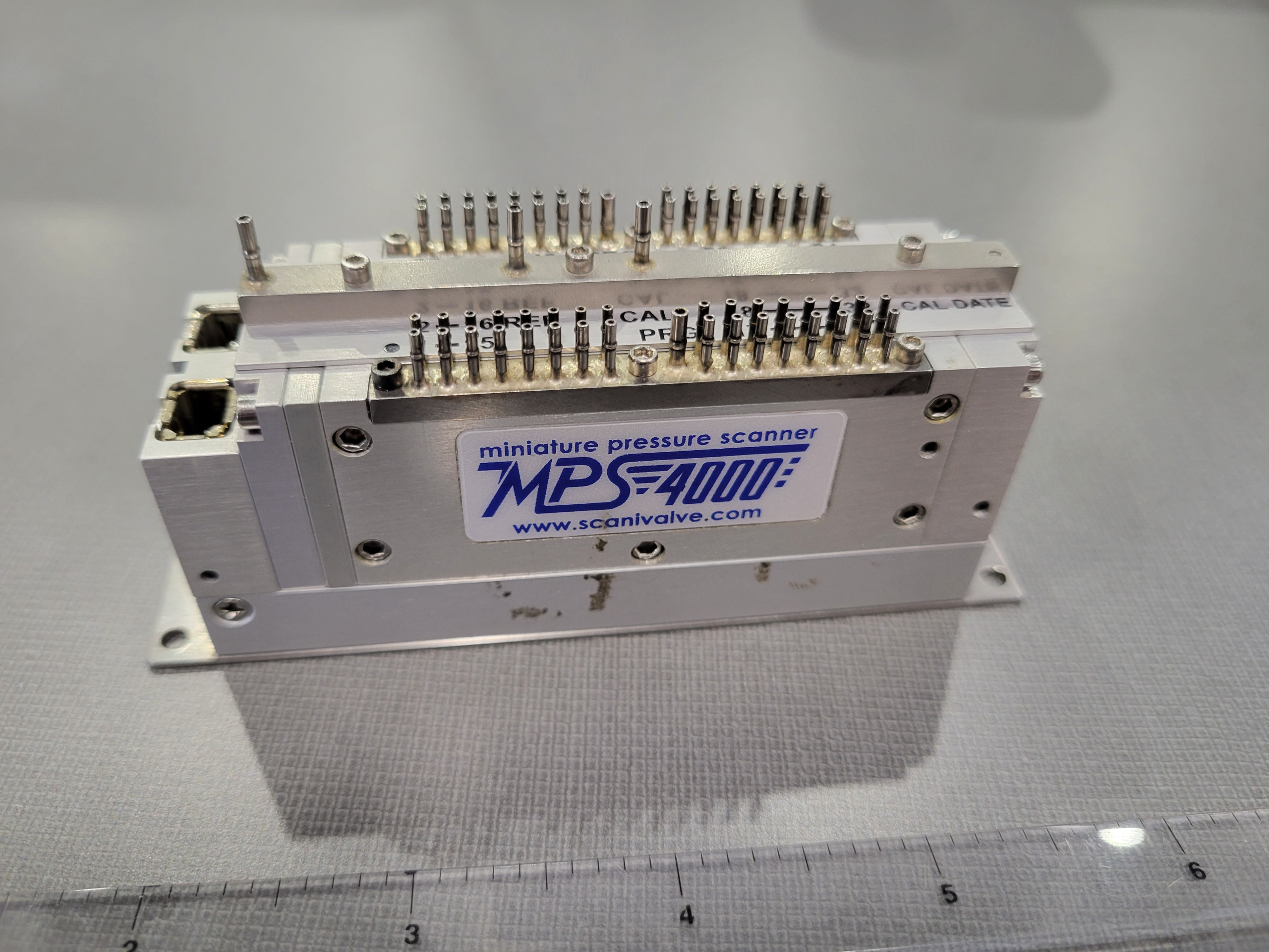
For unsteady or high-speed flows, conventional tubing systems may introduce phase lag and damping. In such cases, fast-response transducers are mounted close to the surface to minimize pneumatic delay, enabling the accurate measurement of rapid pressure fluctuations such as those in buffet, vortex shedding, or aeroacoustic studies. In this case, each transducer is connected to a suitable signal conditioning system before being digitized and stored on a computer. Each pressure transducer must be individually calibrated, which is usually conducted in-situ.
In recent decades, pressure-sensitive paint (PSP) techniques have become increasingly valuable. PSP is applied as a thin, luminescent coating on the model surface. When illuminated, its emission intensity varies with the partial pressure concentration of oxygen, which is directly related to the surface pressure. The pink paint shines when exposed to blue light, glowing brighter or dimmer depending on the air pressure in the area. This method provides full-field pressure maps with high spatial resolution, allowing detailed visualization of flow structures that would be difficult to measure with discrete taps alone. However, PSP requires careful calibration, is sensitive to temperature, and typically demands low-turbulence optical environments for best accuracy.
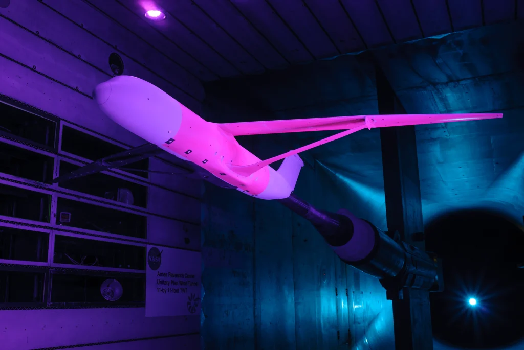
Flow Visualization
Flow visualization techniques are widely used in wind tunnels in conjunction with quantitative measurements to provide a deeper insight into aerodynamic behavior. These methods are among the most immediately satisfying measurement approaches because they reveal features such as boundary-layer separation, vortex formation, shock structures, and streamline patterns. These features may not be apparent from force or pressure data alone, thereby enhancing both experimental interpretation and the communication of results, such as in reports and papers.
Smoke & Dye Injection
Smoke and dye injection introduce visible tracers into the flow to highlight streamline paths, vortex shedding, or regions of recirculation. Smoke filaments or dye streaks make unsteady structures directly observable, though seeding can sometimes disturb delicate low-speed flows. The image shows a scale model of an F/A-18 aircraft inside the NASA Dryden Flow Visualization Facility. Colored dyes are pumped through tubes equipped with needle valves, then released at strategic points on the surface. The dyes then flow back along the airframe and over the wings, highlighting their aerodynamic characteristics.
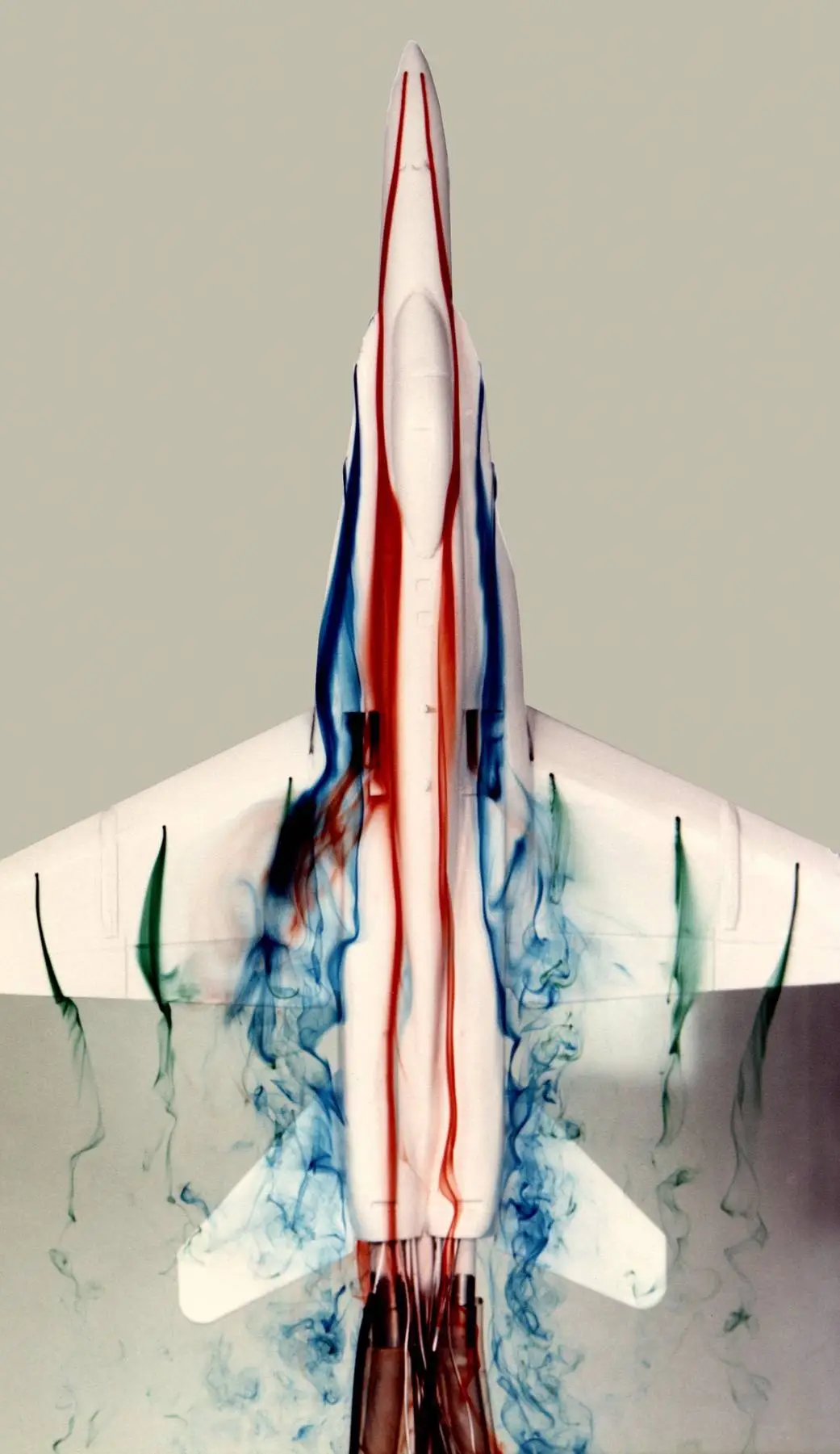
Surface Oil-Flow Visualization
Oil-flow visualization involves applying a thin film of low-viscosity oil, often mixed with a pigment or dye, to the model’s surface. Using high-quality mineral oil with titanium dioxide powder or white emulsion paint is a common approach. As the flow shears the film, the oil is redistributed or blown off, leaving white streak patterns that reveal regions of attachment, separation, and reattachment. Painting the surface black gives maximum contrast. An example is shown in the image below, depicting the complex regions of flow separation on the superstructure of a generic Navy ship.
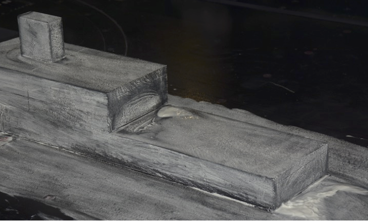
These surface patterns offer excellent insight into local shear stresses and also help researchers gain a deeper understanding of integrated aerodynamic behaviors, such as lift and drag. A fluorescent type of oil can also be used; when illuminated with ultraviolet light, it produces high-contrast patterns that enhance the visibility of subtle flow features. However, oil-flow methods require careful lighting and high-resolution imaging to image the details effectively. The use of filters for visible light on the camera lens further improves contrast.
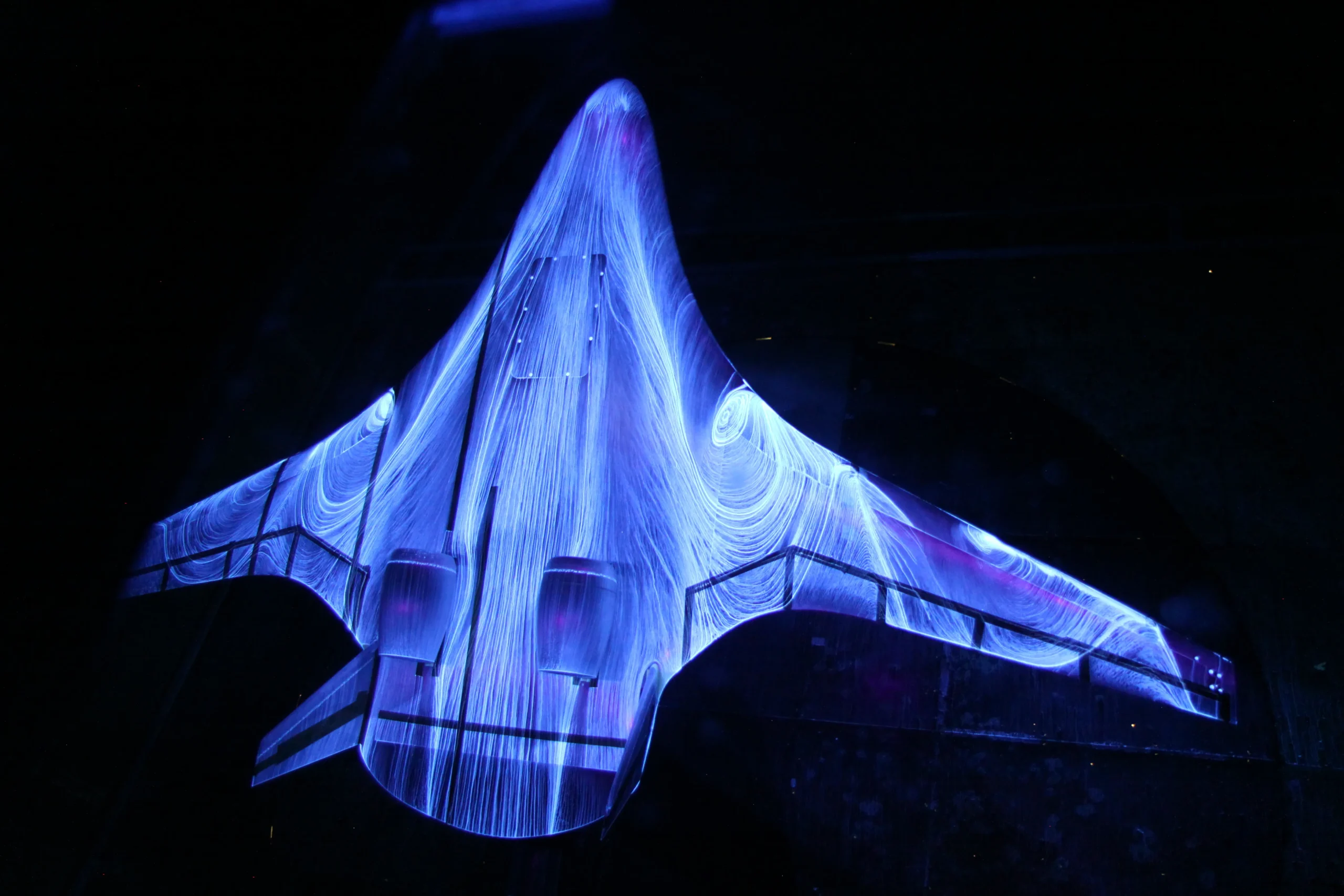
Tufts
Tufts are small strands of yarn or ribbon attached to the surface of the wind tunnel model, providing a reliable and straightforward indication of local flow direction, attachment, or separation. They are inexpensive and easy to interpret, but they do not provide as much detail as oil flow methods, and they must be applied sparingly to avoid disturbing the boundary layer. Nevertheless, they are quick and easy to apply. They can be quite helpful for identifying regions of flow separation and cross-checking other measurements, such as wings near the onset of stall, as shown in the photograph below.
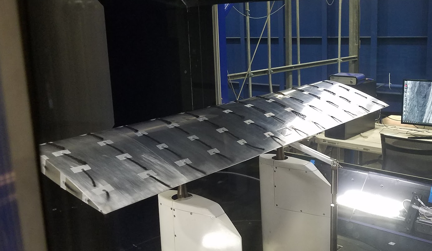
A refinement of this method uses fluorescent minitufts, which are short polyester monofilament fibers soaked in a UV-sensitive dye and glued to the surface. Under flow, the minitufts align with the local direction. When illuminated by a UV flash, they fluoresce, appearing brighter and more visible, which significantly improves the clarity of flow visualization in photographs and videos.
Schlieren & Shadowgraph
Schlieren and shadowgraph are techniques that exploit variations in refractive index caused by density gradients in the flow, making compressibility effects such as shock waves, expansion fans, and shear layers visible. Such methods are widely used in high-speed wind tunnels but can also be applied at lower speeds, depending on the flow. For example, the high-speed wake behind jet engines and the tip vortices of propeller and helicopter rotors are often visualized using such density gradient methods.
The connection between optical measurements and aerodynamic flow fields is provided by the Gladstone-Dale relation, i.e.,
(73) 
where  is the refractive index of the gas,
  is the local density, and
  is the Gladstone-Dale constant. This constant depends weakly on gas composition and the wavelength of light used. For air at standard conditions in the visible spectrum,
  m
m /kg. Although is typically of order
  , it is directly proportional to , making even small density variations optically detectable.
To describe the geometry, let denote the line-of-sight (LOS) direction of the optical system, the horizontal axis in the image plane, and  the vertical axis in the image plane. Small variations in refractive index bend light rays passing through the flow. For weak gradients and small deflections, geometric optics gives
(74) 
where  is the ambient refractive index and is the line-of-sight coordinate. Using the Gladstone-Dale relation, these become
(75) 
These deflection angles provide the physical connection between flow density variations and what is seen on the camera.
In schlieren systems, these angular deflections are converted into brightness variations by a knife-edge or filter at the focal point, so even weak shocks or thermal plumes become visible. The system utilizes a point light source and one or two spherical or parabolic mirrors, which must be optically aligned with care. A single-mirror system is illustrated in the figure below.

Flow visualization methods for compressible flows include schlieren (sensitive to first density derivatives) and shadowgraphy (sensitive to second derivatives).
The quality of the alignment determines sensitivity. Even a slight misplacement of the knife edge or source can blur the image or reduce contrast. The measured light intensity is proportional to the LOS integral of the first derivative of density, i.e.,
(76) 
where  is the direction perpendicular to the knife edge. Therefore, by rotating the knife edge, one can choose whether to emphasize vertical or horizontal density gradients. Schlieren, therefore, highlights smooth but extended density gradients, such as those found in boundary layers, shear layers, wakes, and shock structures, with an example shown in the image below. With pulsed light sources or high-speed cameras, schlieren can also capture the unsteady motion of shock waves, vortex shedding, and other unsteady phenomena.
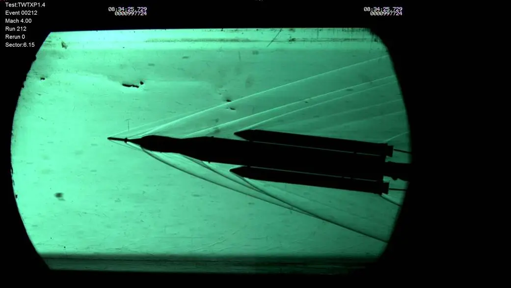
Shadowgraph systems rely on the same physical ray deflections but record the curvature of the rays instead of their angles. In practice, light passes through the test section and onto a retroreflective screen, which is designed to reflect the rays back toward their source. Rertroreflector material comes in large, self-adhesive plastic sheets so that they can be applied to almost any surface. Refraction effects in the flow deflect the rays so that they no longer perfectly retrace their paths, and these deviations are imaged on the camera after passing through a beamsplitter plate. The measured intensity is proportional to the LOS integral of the second derivative of density,
(77) 
which makes shadowgraphy especially sensitive to sharp, localized gradients such as shocks, expansion fans, and shock-boundary layer interactions. Because the signal depends on the curvature of the density field, shadowgraph images emphasize discontinuities but may lose detail in more gradual density variations.
Nevertheless, shadowgraph systems are easier and less expensive to set up than schlieren, require fewer optical elements (no mirrors), and provide a much wider field of view (they are not limited to the diameter of a minor) while still revealing most of the same compressible-flow phenomena. For this reason, they are widely used in supersonic and hypersonic testing, particularly where simplicity and robustness are needed.
Velocity Field Measurements
A variety of techniques are used to measure velocity fields and visualize flow structures in wind tunnel testing. Pitot-static probes provide local estimates of mean flow speed by comparing total and static pressures, and they remain a standard method for quick surveys of velocity distributions. Hot-wire and hot-film anemometry enable the resolution of fine-scale velocity fluctuations and turbulence intensity, with a very high frequency response. However, they require careful calibration and are intrusive in the flow.
5- and 7-Hole Probes
Multi-hole probes are used to measure local flow direction and velocity components by resolving the pressure distribution around a small sensing head. They are especially valuable in three-dimensional or swirling flows where a conventional Pitot-static tube cannot measure the velocity vector.
A 5-hole probe consists of a central tube surrounded by four peripheral pressure ports, arranged typically in a cruciform pattern. The central port measures a stagnation-like pressure, while the peripheral ports sense pressure differences that vary with yaw and pitch angle. By calibrating the probe in a known flow field, the measured pressure coefficients can be related to the local magnitude of the flow velocity and its angular orientation. 5-hole probes are therefore capable of resolving the three velocity components ( ) at a point.
A 7-hole probe extends this principle by adding two additional ports, usually arranged in a hexagonal pattern around the central port, as shown in the figure below. The additional ports enhance sensitivity and angular range, thereby improving accuracy for flows with large incidence angles or strong cross-flow components. However, they cannot resolve separated regions where turbulent energy is dissipated into heat rather than appearing as recoverable pressure.
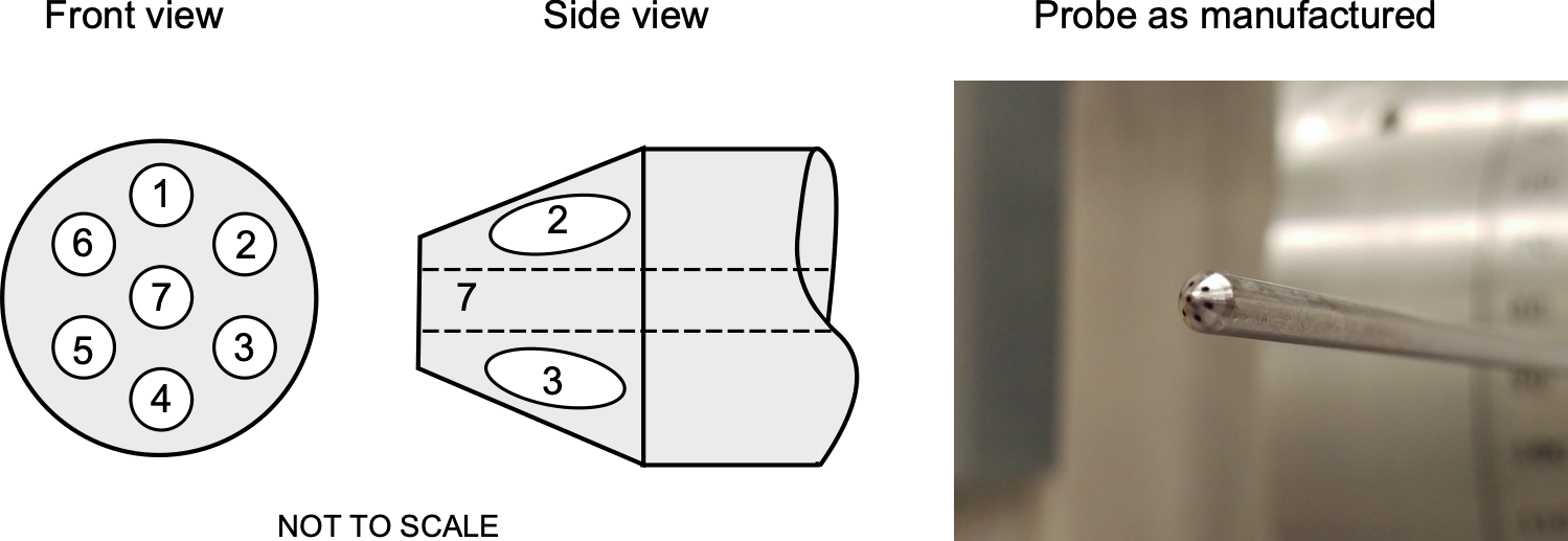
The general principle is to relate the pressure distribution on the probe head to the local flow direction and the magnitude of the velocity. During calibration, the probe is placed in a uniform reference flow and systematically yawed and pitched through a range of angles. At each orientation, the pressures from the central and peripheral ports are recorded. From these data, calibration functions are built that link the measured pressure differences to flow angles.
A common definition is to form non-dimensional pressure coefficients relative to the central port,
(78) 
where  is the pressure at peripheral port
  ,
,  is the central port pressure, and
  is the reference dynamic pressure. Suitable combinations of these coefficients, such as
(79) 
are then correlated to the local pitch angle and yaw angle  of the flow. The total velocity magnitude can be obtained from the calibrated relation between the central port pressure (or a weighted average of all ports) and the reference freestream pressure. In practice, these calibration functions are stored as multi-dimensional lookup tables or polynomial fits. When the probe is used in an unknown flow, the measured set of pressures is converted into velocity components
  by interpolating within the calibration map.
Although intrusive, the probes are manufactured from very fine hypodermic stainless-steel tubing with diameters often less than a millimeter. This allows the probe head to be extremely small, minimizing flow disturbance and permitting measurements in regions with significant velocity gradients. However, pressure probes have limited frequency response because the port-tubing-transducer system acts as a low-pass filter. While they can track slow variations in flow angle or magnitude, they cannot capture the effects produced in unsteady flows. As a result, they are best suited for steady or quasi-steady flows.
Additionally, pressure probes (multi-hole or otherwise) cannot fully resolve regions that are either completely separated or highly turbulent. In such flows, the assumptions of Bernoulli’s equation break down because total pressure is no longer conserved along a streamline. A portion of the mechanical energy is extracted into turbulent losses, which do not appear as recoverable pressure at the probe ports. Because a Pitot probe depends on interpreting measured pressure distributions as indicators of velocity direction and magnitude, it loses validity once the flow becomes separated.
This limitation can be expressed directly from the mechanical energy equation. For steady, incompressible flow along a streamline without losses, Bernoulli’s equation is
(80) 
Here, any change in velocity is reflected as a corresponding change in pressure, allowing the probe to infer the velocity vector from measured pressure differences. When separation or strong turbulence is present, however, an additional loss term must be included, i.e., in this case
(81) 
where  represents the irreversible conversion of mechanical energy into turbulence and heat. In terms of stagnation pressure, then
(82) 
showing that the total pressure sensed by the probe is reduced. Because the calibration of 5- and 7-hole probes assumes negligible loss, the pressure distribution no longer maps uniquely to a velocity vector.
Multi-hole probes are robust and relatively easy to use. However, they require careful calibration, have a limited frequency response compared to optical or hot-wire methods, and can still perturb sensitive flows. Their use in unsteady and/or separated flows (like a wake) should be avoided. Nevertheless, despite their limitations, they remain widely used in wind tunnel applications for mapping three-dimensional flow fields with reasonable accuracy.
Hot-Wire Anemometry (HWA)
Hot-Wire Anemometry (HWA) is a non-intrusive measurement technique widely used in experimental aerodynamics for resolving velocity fluctuations, particularly in turbulent flows. The method relies on the principle that the convective heat loss from a thin, electrically heated wire is directly related to the local flow velocity.
A very fine wire (often platinum or tungsten, with diameters of a few microns) is electrically heated above the ambient air temperature. They come in single, two-component, and three-component forms. An example of a three-component wire is shown in the photograph below, where the wires are supported between two prongs. As the airflow passes over the wire, it cools the wire by forced convection. To maintain a constant temperature (CTA = Constant-Temperature Anemometer) or to measure the changing resistance (CVA = Constant-Voltage Anemometer), the electrical circuit must supply power in proportion to the local flow velocity.
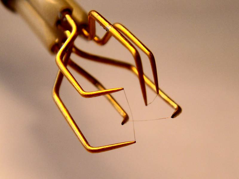
The response depends on the heat-transfer relationship from the wire, which can be written as King’s law to empirically relate the mean square of the wire voltage to the velocity magnitude, i.e.,
(83) 
where  is the measured voltage across the wire,
  is the local velocity, and ,
  , and are calibration constants determined experimentally, usually by calibrating in a small jet flow.
Because of the minimal thermal inertia of the wire, hot-wire anemometers can resolve velocity fluctuations at very high frequencies (tens of kHz or higher), making them extremely useful for turbulence research. However, the technique is limited to gases, requires careful in situ calibration, and the fragile wires can break easily under high turbulence intensity, dust, or particle-laden flows.
Laser Doppler Velocimetry (LDV)
Laser Doppler Velocimetry (LDV) is a non-intrusive technique that measures local flow velocities by detecting the Doppler frequency shift of laser light scattered by small seeding particles that follow the flow. Two coherent laser beams are made to intersect at a small ellipsoidal volume, forming an interference fringe pattern. As they pass through this volume, the scattered light is modulated at a frequency proportional to the velocity component along the bisector of the beams, which can be detected using a suitable optic and a photomultiplier.
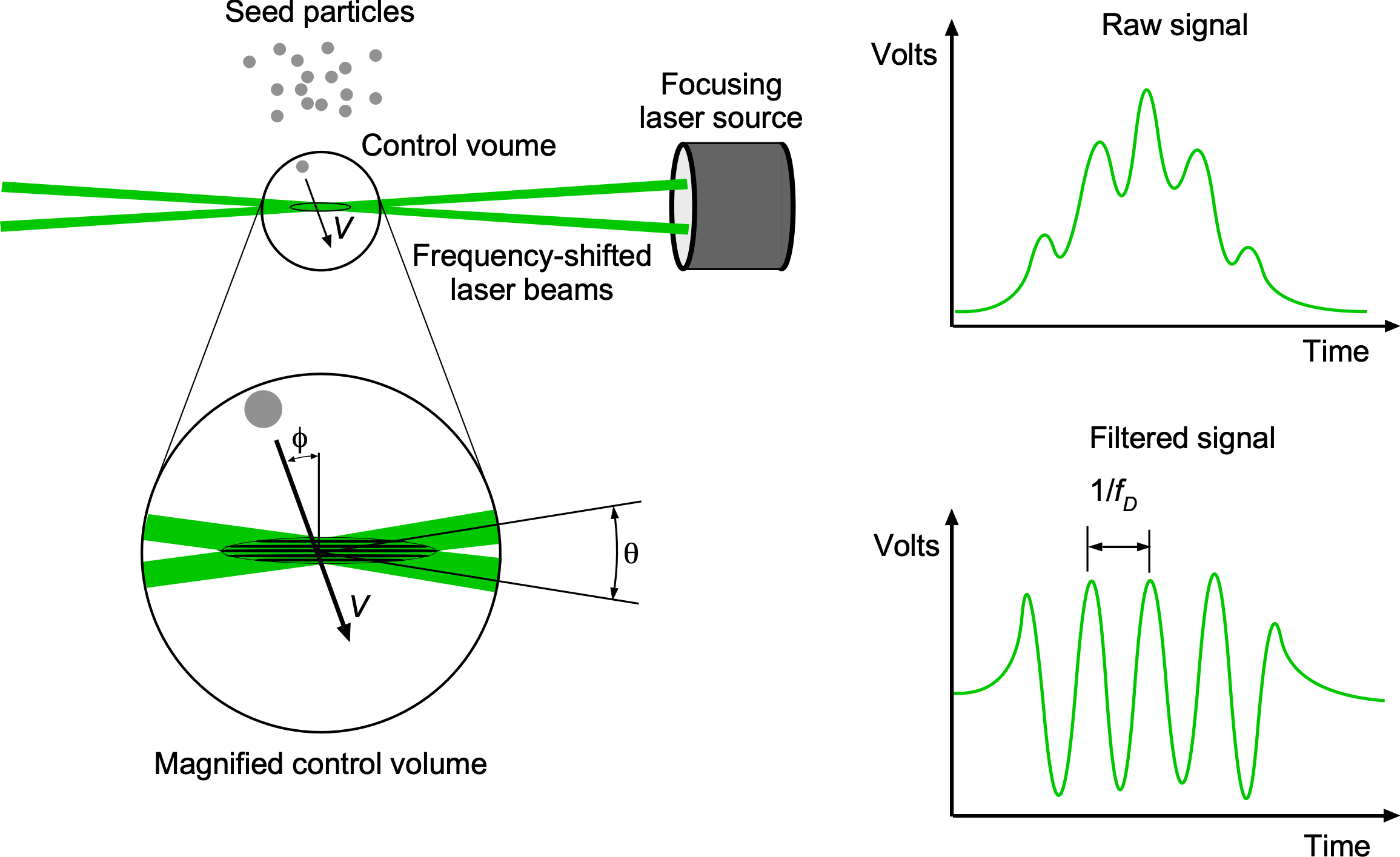
The fringe spacing is given by
(84) 
where is the wavelength of the laser beams and is the intersection angle between the beams. The measured Doppler frequency is
(85) 
where is the particle velocity and  is the angle between the particle trajectory and the fringe pattern. Therefore, the velocity component along the measurement axis can be determined from
(86) 
By measuring this frequency with a photodetector, the instantaneous velocity at that point can be determined with very high spatial and temporal resolution, which is significantly higher than currently possible with PIV.
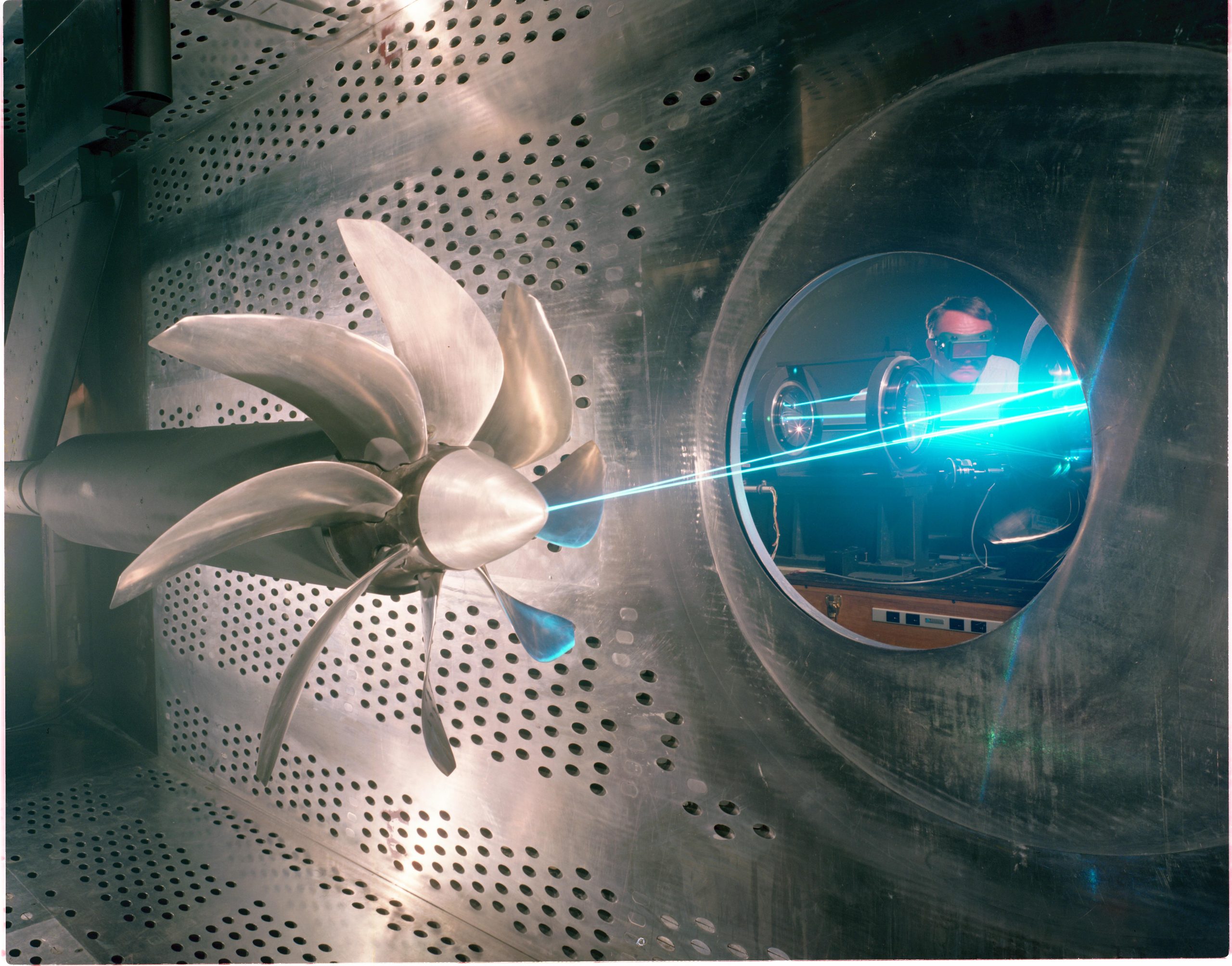
Multi-component LDV systems are obtained by adding additional beam pairs, which are created by splitting the primary wavelength (usually green) into blue, indigo, and violet wavelengths and frequency-shifting one of the beam pairs. This allows discrimination of direction and enables simultaneous measurement of two or three orthogonal velocity components. LDV is particularly valuable in turbulent-flow research, where accurate pointwise velocity measurements are needed without disturbing the flow field. Measurement volumes of the order of 80 m are possible, which is thinner than the thickness of a human hair.
Particle Image Velocimetry (PIV)
Particle Image Velocimetry (PIV) has largely replaced LDV and extends this capability to entire flow fields, capturing two-dimensional or volumetric velocity maps. In PIV, seeded particles are illuminated by a thin laser sheet and tracked between successive camera exposures, allowing velocity vectors to be reconstructed across the illuminated region. High-speed PIV can accurately resolve unsteady flow phenomena, including vortex shedding, separation, and wake interactions.
In PIV, the flow is seeded with tracer particles and illuminated by a pulsed laser sheet. Two successive images are recorded by a high-resolution camera, as shown in the schematic below. The displacement of particle groups between the exposures is obtained using cross-correlation techniques, yielding velocity vectors over the illuminated region. With appropriate optics, this approach provides planar or even volumetric maps of the velocity field, offering excellent spatial coverage. High-speed PIV systems allow the measurement of rapidly evolving flow structures, making the method compelling for studying turbulence, vortex shedding, separation bubbles, and unsteady wake dynamics.
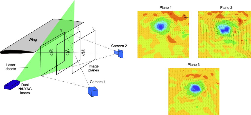
The basic relation for obtaining the velocity field from measured particle displacements is
(87) 
where  is the measured particle-image displacement vector and
  is the known time delay between exposures, which is typically very small, of the order of 10 s. More formally, the cross-correlation function in an – plane is
(88) 
with  and
and  denoting the recorded particle images, the method is used to locate the peak corresponding to the most probable particle displacement. The velocity fields can then be determined after further numerical processing.
Model Deformation & Aeroelastic Measurements
For flexible or lightweight models, it is essential to quantify deformation under aerodynamic loading. Several optical and embedded-sensor techniques are available for this purpose. Stereo photogrammetry and laser scanning methods track surface displacements in real time, reconstructing model shape changes throughout the test.
More recently, Digital Image Correlation (DIC) has become widely used for structural measurements in wind tunnels. DIC employs one or more high-resolution cameras to record a random speckle pattern applied to the model surface, as shown in the photograph below. By analyzing pairs of images with cross-correlation algorithms, full-field surface displacements and local strains can be resolved with high spatial accuracy. This non-intrusive technique enables the measurement of both static and dynamic deformations without altering the model’s structure. Conceptually, DIC is similar to particle image velocimetry (PIV). At the same time, PIV tracks seeded particles in the flow to determine velocity fields, DIC tracks speckle features on the model surface to determine deformation and strain fields.
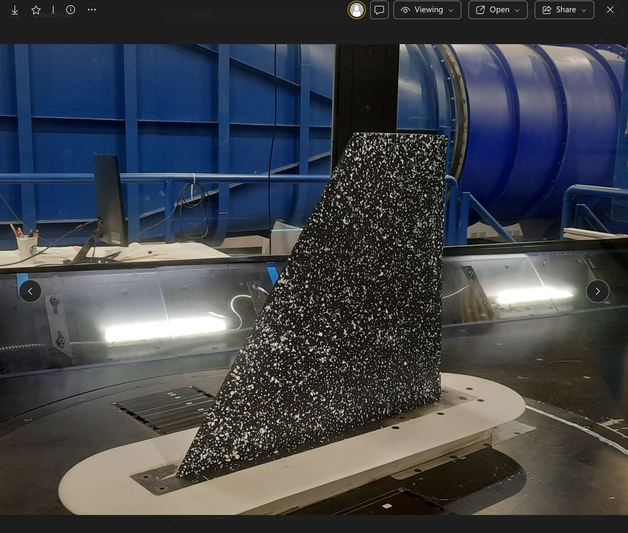
From the measured displacement fields, strain components can be determined directly. For a three-dimensional displacement field,  , the normal strain components are
(89) 
and the shear strains are
(90) 
Here,  ,
,  , and
, and  represent the measured displacement components in the , , and directions, respectively.
It is essential to note that two-dimensional DIC recovers only the in-plane displacements  and corresponding strain components, making it particularly suitable for thin, flat specimens viewed normal to the surface. In contrast, three-dimensional DIC employs at least two synchronized cameras to reconstruct the out-of-plane displacement , allowing full recovery of the strain tensor and enabling accurate measurements of complex structural deformation in wind tunnel models.
Complementing optical methods, strain gauges bonded to critical structural locations provide direct measurements of local strain. Modern facilities also employ fiber optic sensors, such as fiber Bragg gratings, which can be embedded within the model to record distributed strain histories. These embedded techniques are particularly valuable for real-time aeroelastic analysis and for the development of active control systems, where rapid response to structural feedback is required.
Flutter Testing
Flutter testing in a wind tunnel is an important branch of experimental aeroelasticity, but it is also inherently risky because a failure can damage both the model and the facility. Flutter is a dynamic instability that arises from the interaction of aerodynamic, elastic, and inertial forces. When these forces act in phase, the motion can become self-excited, and oscillations may increase in amplitude until structural failure occurs. The purpose of flutter testing is to determine the flutter boundary, defined as the airspeed or dynamic pressure at which the total system damping becomes zero. Tests may also be used to assess active control systems for flutter suppression or to evaluate how changes in stiffness, mass, or aerodynamic configuration affect the aeroelastic stability.
Flutter experiments are typically conducted in transonic or high-speed subsonic wind tunnels where the flow conditions and dynamic pressures are representative of flight, as illustrated in the photograph below. The introduction of thin, highly swept wings during the 1950s raised many new concerns about aeroelastic stability and methods to prevent flutter. Flutter considerations can strongly influence the location of engines, fuel tanks, and other concentrated masses within the airframe. They also play a significant role in determining the required distribution of structural stiffness throughout the wing and fuselage to ensure adequate dynamic margins and to prevent destructive oscillations during flight. NASA Langley’s Transonic Dynamics Tunnel and ONERA’s S2Ch facility are examples of specialized facilities for this type of work. Low-speed tunnels are sometimes used for small-scale models or to investigate control-surface buzz, while supersonic tunnels are employed for missiles and slender wings.
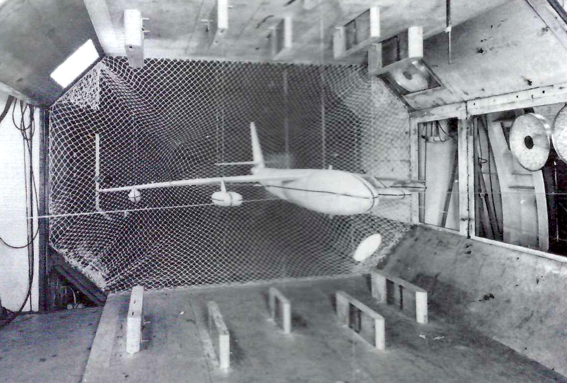
The aeroelastic model must reproduce the essential mass, stiffness, and damping characteristics of the full-scale structure. Ideally, the model satisfies a velocity-scaling relationship that enforces dynamic similarity between aerodynamic and elastic forces. Starting from the Cauchy number, i.e.,
(91) 
where is the flow velocity, is the elastic modulus of the structure, and is the air density, dynamic similarity requires  , i.e.,
(92) 
where the subscripts  and
and  denote the model and full scale, respectively. Solving for the velocity ratio gives
(93) 
This same result can be expressed in terms of the dynamic pressure  , i.e.,
(94) 
The matching of  (or equivalently
  ) is necessary but insufficient for flutter similarity. The structural dynamics must also scale so that the relevant natural frequencies and mode shapes match, i.e., the bending and torsion modes are the same. For a geometrically similar model with a characteristic length , a representative natural frequency
  scales as
(95) 
where  is the material density of the structure. Preserving the reduced frequency
  , which is a characteristic length scale, such as wing chord, then introduces the additional constraint that
(96) 
Together with , this ensures that the fluid-structure time scales are matched and that the same coupled modes are engaged at flutter.
Because exact similarity in , , , and geometry is rarely attainable, models are tuned with added masses and tailored flexures so that the principal modes have the correct frequencies and shapes while satisfying, as closely as practical, the (or ) condition. In practice, wind tunnel models are often much more flexible than their full-scale counterparts, and the target is to match the modal content and reduced frequencies of the modes that participate in flutter.
During flutter testing, the wind speed is gradually increased while the motion of the model is recorded. Flutter may be excited by small shakers or by the flow itself. Measurements of displacement, acceleration, and unsteady pressure are used to determine the natural frequencies and modal damping. When the total damping becomes zero, the system reaches the flutter boundary  , where
  is the damping ratio and
  is the critical dynamic pressure. Beyond this point, the oscillations may remain bounded as a limit-cycle oscillation or diverge rapidly depending on the aerodynamic nonlinearity.
Flutter testing in the wind tunnel is performed cautiously because an instability can develop suddenly. Airspeed is increased in small increments near the predicted boundary, and emergency shutdown systems protect the model and tunnel. Nets are often installed downstream of the test section to catch parts that may have detached from the model. Data must be recorded at high sampling rates to capture the onset and growth of oscillations. When the flutter boundary is exceeded, the motion may either diverge to failure or stabilize at a finite amplitude known as a limit-cycle oscillation. Failure of the model is not a good outcome, but it happens, often within a fraction of a second. Such self-sustained motions arise from nonlinear aerodynamic or structural effects and are most common in lightly damped systems. Data from wind tunnel tests are essential for validating models of this nonlinear behavior, especially for configurations with control surfaces, external stores, or other features that alter stiffness and flow separation.
Data Reduction
Raw measurements from wind tunnel tests are rarely usable in their initial form. A systematic process of data reduction and correction is essential to produce results that reflect the model’s aerodynamic behavior under idealized, free-flight conditions. This process accounts for local flow conditions, non-dimensionalization, and known tunnel effects such as wall and support interference. Through calibration, correction, normalization, and uncertainty analysis, raw measurements are transformed into high-fidelity aerodynamic data that can be compared with theory, CFD, or flight tests and scaled to full-flight conditions. The process of data reduction can take a considerable amount of time and must be factored into estimates of the overall time needed for a wind tunnel test campaign.
Non-Dimensionalization of Data
The first step is to non-dimensionalize the measured data, such as pressures, velocities, forces, and moments. Aerodynamic coefficients are obtained by normalizing with respect to the freestream dynamic pressure in the usual way. The dynamic pressure is
(97) 
where is the freestream density and the freestream velocity. For example, the lift and moment coefficients are
(98) 
where is the lift, is the pitching moment,  the reference area, and
  the reference chord. Similar expressions define the other force and moment coefficients. Moments reported about one reference point may be transferred to another using the principles of statics, so it is essential to state the reference geometry and sign conventions.
Corrections
Corrections for wall interference on balance data are another essential step. Empirical correction charts or numerical models are often required to recover free-flight conditions. Most wind tunnel facilities have standard methods of correction, built over years of testing experience, and these should be followed. In particular, stings, struts, and brackets disturb the flow and introduce spurious forces. Their contribution is quantified by tare measurements with the support hardware alone, which are then subtracted from the full-model data.
Tunnel-effect corrections typically include solid and wake blockage, wall-interference induced angle of attack and force/moment coefficient adjustments, buoyancy (if relevant to the force component being inferred from a balance in air), and support (sting/strut) interference. The angle-of-attack should be checked and calibrated if needed, e.g.
(99) 
from facility flow-angularity surveys or in situ pressure-rake calibrations.
Uncertainty Analysis
Ultimately, a comprehensive uncertainty analysis is necessary. for all of the measured data. This is an important step that is often overlooked, but essential if the data are to be published. Each measured or derived quantity carries uncertainty, and these uncertainties propagate into the aerodynamic parameters and coefficients. For example, a function  , the combined standard uncertainty is given by
(100) 
for uncorrelated inputs, with covariance terms added if correlations exist. In reporting, it is common to present the expanded uncertainty, i.e.,
(101) 
where  is the coverage factor, typically = 2 for a 95% confidence level. This provides a transparent confidence interval around the reported aerodynamic coefficients and other data.
Uncertainties should distinguish Type A (statistical) and Type B (systematic) components and, when selecting the coverage factor , use an effective degrees of freedom (e.g., Welch-Satterthwaite) to reflect finite sample sizes and correlated inputs (notably all those entering into the values of  ).
).
Test Planning & Execution
Let’s do a wind tunnel test! Wind tunnel testing is a time-consuming and resource-intensive activity that demands meticulous planning to yield meaningful, repeatable, and efficient results. From defining the test goals to preparing a matrix of conditions and executing the test runs, every phase must be carefully orchestrated. Wind tunnel testing is most productive when objectives, hardware, and operations are harmonized in advance. Detailed planning, rigorous execution, and careful quality control ensure that each run contributes reliable data to the overall campaign and maximizes the value of the experimental effort.
Defining Test Objectives
The first step in a successful wind tunnel campaign is to define the test objectives clearly. These may range from measuring aerodynamic force and moment coefficients to doing PIV measurements to validate CFD predictions, examining the effectiveness of control surfaces, or studying complex phenomena such as flow separation, shock formation, or aeroacoustics. The clarity and specificity of the objectives inform the design of the test article, the choice of instrumentation, and the data analysis methods. A carefully prepared pre-proposal is required, which can then be refined into a full proposal after input from the wind tunnel staff.
Model Design & Preparation
Model design is a balance between geometric accuracy, structural integrity, and test utility. The chosen scale and aspect ratio influence the Reynolds number and susceptibility to wall effects. A smooth surface finish ensures predictable boundary layer development, while internal arrangements must accommodate pressure taps, wiring, and mounting hardware. Modular construction enables rapid configuration changes, such as swapping control surfaces or simulating various flight conditions. Precision in manufacturing and documentation is critical to ensure consistency across test campaigns.
Equally important is structural design. Wind tunnel models are subjected to aerodynamic loads, inertial forces from mounting systems, and sometimes dynamic oscillations. In the case of a drone, just because it can fly does not mean that it would survive a wind tunnel test without structural modification. Stress analysis must, therefore, be carried out to verify that the model can withstand the maximum expected test loads in the wind tunnel. All wind tunnels have factor of safety rules. The factor of safety (FOS) is defined as
(102) 
where  is the failure stress of the material and
  is the maximum applied stress during testing. Conservative factors of safety are typically chosen, often ranging from 2 to 4, depending on material properties, structural complexity, and the uncertainty in load prediction. Lower or higher values of FOS may be used depending on the projected risk to the wind tunnel facility.
Before any model is allowed into the test section, it must undergo thorough bench testing. Bench testing involves applying known static (and perhaps dynamic) loads to verify the structural strength, stiffness, and integrity of instrumentation under controlled conditions. This step ensures that the model will not fail catastrophically inside the tunnel, where damage to the facility and risk to instrumentation would be severe. Bench testing also allows for the identification of weak points, calibration of any strain gauges on the model, and validation of the mounting arrangements.
Lightweight models intended for testing must strike a careful balance between stiffness and mass to avoid excessive deformation, while flexible models designed for aeroelastic studies require controlled compliance. In either case, the combined application of stress analysis, conservative safety margins, and bench testing ensures that models will deliver reliable results without risk of structural failure during wind tunnel operation. Safety of flight strain gauges may be required and monitored during the tests to ensure that the loads remain below critical levels.
Instrumentation & Facility Setup
The instrumentation suite and facility configuration must always be tailored to the specific objectives of any given wind tunnel test. Careful planning and verification of the instrumentation and facility configuration, therefore, underpin the accuracy, repeatability, and ultimate usefulness of wind tunnel data. This process begins with the installation and careful calibration of balances, pressure sensors, and flow meters or probes to ensure reliable measurements. The model itself must be precisely aligned with the tunnel axis and coordinate system, as even small misalignments can introduce systematic errors in the measured forces and moments.
Freestream conditions, including velocity, temperature, and turbulence intensity, must be verified and documented before testing to establish a reliable reference state. Data acquisition systems are configured to sample at rates sufficient to measure the relevant flow phenomena, with filtering applied to suppress noise while preserving the signal content. Synchronization between model instrumentation and tunnel operating conditions is crucial, especially during tests where unsteady components need to be measured.
Reference frames and sign conventions must be standardized across the test campaign. Without this discipline, even well-executed measurements can be misinterpreted. In addition, a system health check is usually carried out before running the tunnel, during which the data acquisition system is operated without flow to confirm sensor zeroing, baseline stability, and absence of electrical noise. A typical example is the reversal of angle sweeps, which can lead to systematic errors that propagate throughout the dataset if not detected during pre-test checks.
Test Matrix & Run Schedule
A detailed test matrix provides the framework for the entire experimental campaign by laying out the planned conditions under which the model will be evaluated. This includes the range of angles of attack, sideslip angles, and control surface deflections to be investigated, as well as the freestream Mach and Reynolds numbers to be simulated. Configuration changes such as flap settings, external stores, or alternate geometries must also be incorporated.
Efficient use of tunnel time requires careful scheduling beyond the primary data points. Startup and shutdown periods must be accounted for, along with tare runs to quantify the effects of support and instrumentation. Contingency plans should be included to address unexpected model issues or equipment malfunctions, ensuring that valuable tunnel time is not lost.
Redundancy is also an essential feature of a well-designed test matrix. Repeating selected test points at intervals throughout the campaign allows the experimenter to check data repeatability and identify any drift in instrumentation, flow conditions, or model alignment. By striking a balance between completeness and efficiency, the test matrix ensures that the wind tunnel campaign generates a reliable and representative dataset while maximizing the optimal use of the limited facility time.
Tests that utilize optical flow diagnostics, such as particle image velocimetry (PIV), require substantial setup and calibration, including laser-sheet alignment, camera and lens calibration and mapping, timing synchronization, uniformity checks for seeding, and safety procedures. This preparation often spans several days and must be factored explicitly into the facility schedule and resource plan, not just the allocated run time, to avoid compressing objectives or compromising data quality.
Data Acquisition & Quality Control
During each run, data quality must be continuously monitored in real time. Force and pressure signals are examined for convergence and consistency, while anomalies such as drift, excessive noise, or sudden step changes may indicate malfunctions or setup issues. Flow visualization methods, such as smoke, tufts, or Schlieren, can reveal unexpected behavior, including boundary-layer separation, shock motion, or structural vibration that may not be immediately evident in the balance data.
Repeat runs at identical conditions are routinely performed to assess repeatability and to separate genuine aerodynamic trends from measurement artifacts. Rapid, preliminary (“quick-look”) processing during the test enables early detection of anomalies and allows the plan to be adjusted while tunnel time remains. Entire wind-tunnel campaigns have been ruined when anomalous behavior was only recognized after the tests were completed.
Summary & Closure
Despite major progress in computational aerodynamics, particularly in computational fluid dynamics (CFD), wind-tunnel testing is still essential for design verification and for understanding real aerodynamic behavior. Scale-model testing almost always involves compromises because it is rarely possible to match Reynolds number, Mach number, and structural similarity at the same time. Experienced experimentalists know how to manage these limitations and still obtain reliable and useful trends. Forces, moments, and surface pressures remain the fundamental quantities of interest, but modern facilities now make routine use of optical diagnostics such as particle image velocimetry (PIV), which reveal the three-dimensional structure of wakes, vortices, and separated regions with a level of detail that conventional instrumentation cannot provide.
Wind tunnels provide direct access to the physical flow, something that CFD cannot duplicate. Their design, classification, and operating principles reflect more than a century of accumulated experience in producing uniform, low-turbulence flow for quantitative measurements. Reliable testing requires attention to similarity requirements, wall and support interference, calibration procedures, and the need for uncertainty quantification to establish the credibility of the data.
Effective wind-tunnel work depends on more than the facility itself. Clear objectives, sound model design, proper selection and calibration of instrumentation, and consistent procedures for data reduction are essential. When these fundamentals are handled correctly, wind-tunnel measurements provide the most trustworthy aerodynamic data available and remain the primary reference against which CFD must be judged.
The future of aerodynamic testing will rely on a hybrid approach that combines computation and experiment. Tunnel data provide the basis for validating numerical models, while high-fidelity CFD can explore portions of the parameter space that are difficult or impossible to reach experimentally. Developments such as adaptive-wall test sections, real-time integration of diagnostics with facility controls, and more automated acquisition will continue to improve the quality and efficiency of tunnel testing. Even with continued advances in computation, wind tunnels will remain central to aerospace research and development because they deliver direct and repeatable measurements of the real flow.
5-Question Self-Assessment Quickquiz
For Further Thought or Discussion
- Why do wind tunnels remain essential in aerospace research and development despite the rapid progress of computational fluid dynamics?
- What compromises are involved in model scaling, and why is it often impossible to match both Reynolds number and Mach number simultaneously in a subscale wind tunnel test?
- How does flow quality influence the fidelity of wind tunnel data? Which of the four primary metrics, uniformity, steadiness, turbulence intensity, and angularity, do you think is most critical, and why
- Consider a model with a blockage ratio of 6%. What kinds of errors might this introduce, and what strategies could be applied to mitigate them?
- Discuss the relative advantages and limitations of traditional force balances versus modern optical methods such as particle image velocimetry (PIV) and digital image correlation (DIC). Under what conditions might one method be preferred over another?
- In what ways can boundary layer growth on the walls of the test section distort experimental results? How do area corrections or corner fillets alleviate these effects?
- How do horizontal buoyancy effects arise in a wind tunnel, and why can they matter even when the effect is small in magnitude?
- What role does uncertainty quantification play in wind tunnel testing, and how does it influence the credibility of experimental results when compared with CFD or flight test data?
- Imagine you are tasked with testing a new blended-wing body aircraft. What unique wall interference or scaling challenges would you expect to encounter, and how might you address them?
- Looking to the future, how should wind tunnel testing evolve to complement CFD more effectively? What innovations in tunnel design, diagnostics, or data integration do you anticipate will be most important?
Other Useful Online Resources
Visit the following websites and videos to learn more about wind tunnels and their applications:
- An accessible introduction to the principles and uses of wind tunnels, aimed at students and educators: NASA Glenn — Beginner’s Guide to Wind Tunnels
- An online overview of wind tunnel basics, including the TunnelSim educational software tool: NASA NTRS — Beginner’s Guide to Wind Tunnels
- A full downloadable version with detailed explanations and interactive exercises: NASA NTRS PDF — Beginner’s Guide with TunnelSim
- A gateway to the “Beginner’s Guide to Aeronautics,” with diagrams, activities, and explanations of tunnel operation: NASA Glenn — Wind Tunnel (BGfA landing page)
- A technical paper outlining design principles, classifications, and flow-conditioning strategies for wind tunnels: Cattafesta, Bahr & Mathew — Fundamentals of Wind-Tunnel Design (PDF)
- A demonstration of subsonic tunnel testing for advanced air mobility concepts: YouTube — NASA uses the 14×22 Subsonic Tunnel (Langley AAM test)
- A behind-the-scenes look at the operation and history of the Langley 14×22 wind tunnel: YouTube — Building 1212: NASA Langley 14×22 Wind Tunnel
- A tour of one of the largest and most powerful facilities in the world, used for high-speed aerodynamics research: YouTube — Inside NASA Ames High-Speed Wind Tunnel
- An educational classroom-ready video showing wind tunnels in action: NASA eClips — Wind Tunnels in Action
- Melting Models in Hypersonic Wind Tunnel. A NACA film from the 1960s.
- See: Maxim, H. S., Artificial and Natural Flight, Whittaker & Co., London & New York, 1909. ↵
- Many foundational theories in the field of aerodynamics were established from observations of fluid flows made in the wind tunnel, including lifting line theory. ↵
- Like others, they had followed the work of Otto Lilienthal. They used the “Lilienthal tables, which were based on low-aspect-ratio “bat-like” wings, but these ultimately proved inaccurate for rectangular wings. ↵
- Eastman, J., Ward, K., Pinkerton, R., "The Characteristics of 78 Related Airfoil Sections from Tests in the Variable-Density Wind Tunnel," NACA Technical Report 460, 1933. ↵
- The classic treatments of wall interference and correction methods are given by Allen & Vincenti (1944) and Maskell (1963). ↵
- See Allen, H. J. and Vincenti, W.G., "Wall Interference in a Two-Dimensional-Flow Wind Tunnel, with Consideration of the Effect of Compressibility,'' NACA Report 782, 1944; and Barlow, J.B., Rae, W.H., and Pope, A., Low-Speed Wind Tunnel Testing, 3rd ed., Wiley, 1999. ↵
- Heyson, H. H., ''Jet-Boundary Corrections for Lifting Rotors Centered in Rectangular Wind Tunnels,'' NASA TR R-71, 1960; and Heyson, H. H., ''Ground Effect for Lifting Rotors in Forward Flight,'' NASA TN D-234, 1960. ↵
