19 Thermodynamic Foundations
Introduction[1]
Thermodynamics is the science of energy and the principles governing its transformation from one form to another, such as work and heat, and the production of useful power. It defines the fundamental limits on how energy can be stored, transferred, and converted into useful work. In aerospace engineering, these principles are applied across various contexts, including the aerodynamics of compressible flows and the performance analysis of propulsion systems, ranging from piston and gas turbine engines to rocket engines. Whether analyzing the thrust produced by a nozzle, the work done by a turbine, or the losses incurred in a combustor, thermodynamics provides the unifying basis that connects fundamental physics to practical flight applications.
Engineers in training often first encounter the governing equations of fluid motion, including concepts such as mass, momentum, and energy balances, without realizing that thermodynamics underpins much of their meaning. In particular, gases are compressible, making thermodynamics an intrinsic part of gas dynamics and aerodynamics. Therefore, this chapter presents a concise yet rigorous overview of thermodynamics, focusing on systems, properties, processes, and energy interactions to establish a bridge between fundamental principles and their applications in aerodynamics and other areas of fluid engineering.
At the same time, the subject of thermodynamics can be conceptually and mathematically challenging for most. Many of its difficulties arise because the basic ideas and properties do not always align with intuitive reasoning. For example, even tangible physical quantities such as heat, work, and power are not inherent properties of a system, but rather modes of energy transfer across its boundaries. In contrast, less tangible quantities such as internal energy, entropy, and enthalpy describe the thermodynamic state of the system. Carefully distinguishing between state functions and path-dependent quantities, particularly in describing how systems change from one state to another, is essential in thermodynamics.
The study of thermodynamics must be approached through several complementary avenues, combining mathematical analysis, qualitative reasoning, and illustrative examples. Developing fluency in moving among these perspectives requires time and sustained practice. The most effective path to understanding is to start with the fundamental concepts and their physical meanings, reinforced by straightforward applications like nozzles, diffusers, compressors, turbines, and engines.
Brief History of Thermodynamics
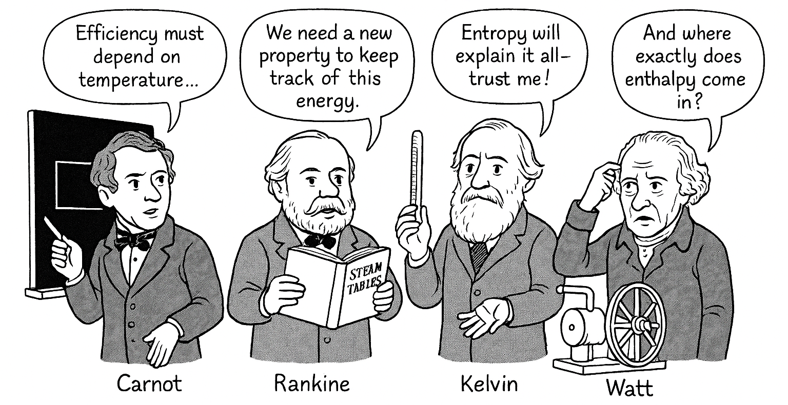
In proceeding, it is helpful to review how the field of thermodynamics emerged and was developed into a physical science, beginning with the earliest types of heat engines. In the seventeenth and eighteenth centuries, inventors such as Denis Papin and Thomas Savery experimented with steam-powered devices. However, it was James Watt who understood the processes of thermal efficiency and transformed the steam engine into a practical machine. This breakthrough led to rapid advances in the field of thermodynamics, marking the beginning of the Industrial Revolution.
In 1824, Sadi Carnot provided the first theoretical framework of thermodynamics by introducing the concept of an idealized heat engine cycle. His insight, that engine efficiency depends solely on the temperature difference between the heat reservoirs, established the principle that no real engine could exceed the efficiency of a reversible thermodynamic cycle.[2] Today, the Carnot efficiency is used as a theoretical ideal of maximum thermodynamic efficiency, but one that no practical engine can ever reach. Rudolf Clausius and William Thomson (Lord Kelvin) later generalized these ideas into the First and Second Laws of thermodynamics by introducing the concepts of energy conservation, internal energy, and entropy. These principles not only helped explain the limits of the existing steam engines of the era but also laid down the universal laws governing all types of energy transformations: energy is always conserved.
By the late nineteenth century, further advances deepened the science of thermodynamics. William John Macquorn Rankine had developed the idealized steam power cycle that bears his name, providing engineers with a mathematical framework for thermodynamic analysis. Josiah Willard Gibbs formalized and extended the mathematical approach, introducing the concepts of free energy and equilibrium criteria. James Clerk Maxwell connected microscopic molecular behavior to the macroscopic properties, establishing the statistical foundation of modern thermodynamics. By the beginning of the 20th century, the field of thermodynamics had matured into a universal physical science with applications of Maxwell’s and Rankine’s mathematical principles extending beyond engines to chemistry and chemical equilibrium, as well as other fields.
| Period | Milestone |
|---|---|
| 1700s | Papin and Savery build early steam-powered devices. James Watt (1769) perfected the steam engine, establishing bounds on efficiency and quantifying power production. |
| 1824 | Sadi Carnot introduces the idealized heat-engine cycle; efficiency depends only on the temperature difference between the heat reservoirs. |
| 1850s–1860s | William John Macquorn Rankine develops the Rankine cycle (ideal vapor power cycle) and publishes a foundational textbook on thermodynamics. Together with Clausius and Kelvin, he establishes the First and Second Laws of Thermodynamics. |
| 1870s | Josiah Willard Gibbs develops the mathematical framework of thermodynamics, including the concepts of free energy and equilibrium criteria. |
| 1870s–1880s | James Clerk Maxwell establishes the field of statistical mechanics, linking microscopic molecular behavior to macroscopic thermodynamic properties. |
| 1900s | Thermodynamics extends beyond engines to chemistry and radiation (blackbody radiation, radiation pressure, entropy of radiation fields). |
| Early 1900s | Thermodynamic cycles applied directly to aviation and aerospace problems: Otto and Diesel (piston engines), Brayton (gas turbines). |
| Mid–1900s | Numerous applications to aerodynamics and high-speed compressible flows, shock waves, and rocket propulsion. |
As the field of aeronautical engineering rapidly evolved in the early twentieth century, these thermodynamic principles were directly applied to the development of more efficient propulsion systems. The Otto and Diesel cycles were used to explain the limits of reciprocating piston engines and to develop means to improve their performance, such as supercharging. The Brayton cycle provided the theoretical foundation for gas turbines, which became the key to understanding jet propulsion and, in turn, to the development of high-speed airplanes. Thermodynamic analyses also proved essential for understanding compressible flows about wings and aircraft, the formation of shock waves, and the behavior of gases at extreme temperatures and pressures encountered in hypersonic flight. For rocketry, extensions of thermodynamic principles guided the design of combustion chambers, nozzles, and staged cycles capable of operating in the vacuum of space.
Today, the same fundamentals remain central to the field of aerospace engineering. From the performance of a small piston engine to the thermal management of scramjets and reusable rocket engines, thermodynamics continues to provide the essential framework for analyzing and optimizing propulsion systems and expanding the boundaries of flight.
Learning Objectives
- Classify thermodynamic properties, and define states and equilibrium conditions.
- Appreciate the significance of the Zeroth Law of Thermodynamics and its role in defining temperature and thermal equilibrium.
- Differentiate between state functions and path functions, and describe how processes are represented.
- Define internal energy, enthalpy, specific heats, and the ratio of specific heats, and understand how to apply them to perfect gases.
- Appreciate the origins of the ideal-gas laws for air and other gases and understand their limitations.
- Understand the significance of the First and Second Laws of thermodynamics and how they are used.
- Relate fundamental thermodynamic concepts to aerospace flow devices such as diffusers, compressors, turbines, combustors, and nozzles.
- Gain an appreciation of combustion thermodynamics and statistical thermodynamics.
Roadmap of Thermodynamics
Thermodynamics is a broad subject, and its concepts build naturally from basic definitions to complex engineering applications. To this end, a roadmap can be helpful for those learning the field. This chapter of the eBook begins with the fundamentals, including systems and control volumes, property classification, and the definitions of states and equilibrium. With these in place, the discussion proceeds to the mechanisms of energy transfer in the form of heat and work, leading directly to the First Law of Thermodynamics and its application to both closed and open (flow) systems. The roadmap below illustrates this progression, showing how each topic connects to the next in the broader framework of thermodynamics. While this chapter does not cover every aspect of thermodynamics, the roadmap is designed to help establish a foundation before moving on to the equations of motion for a fluid and exploring their applications to real engineering problems.
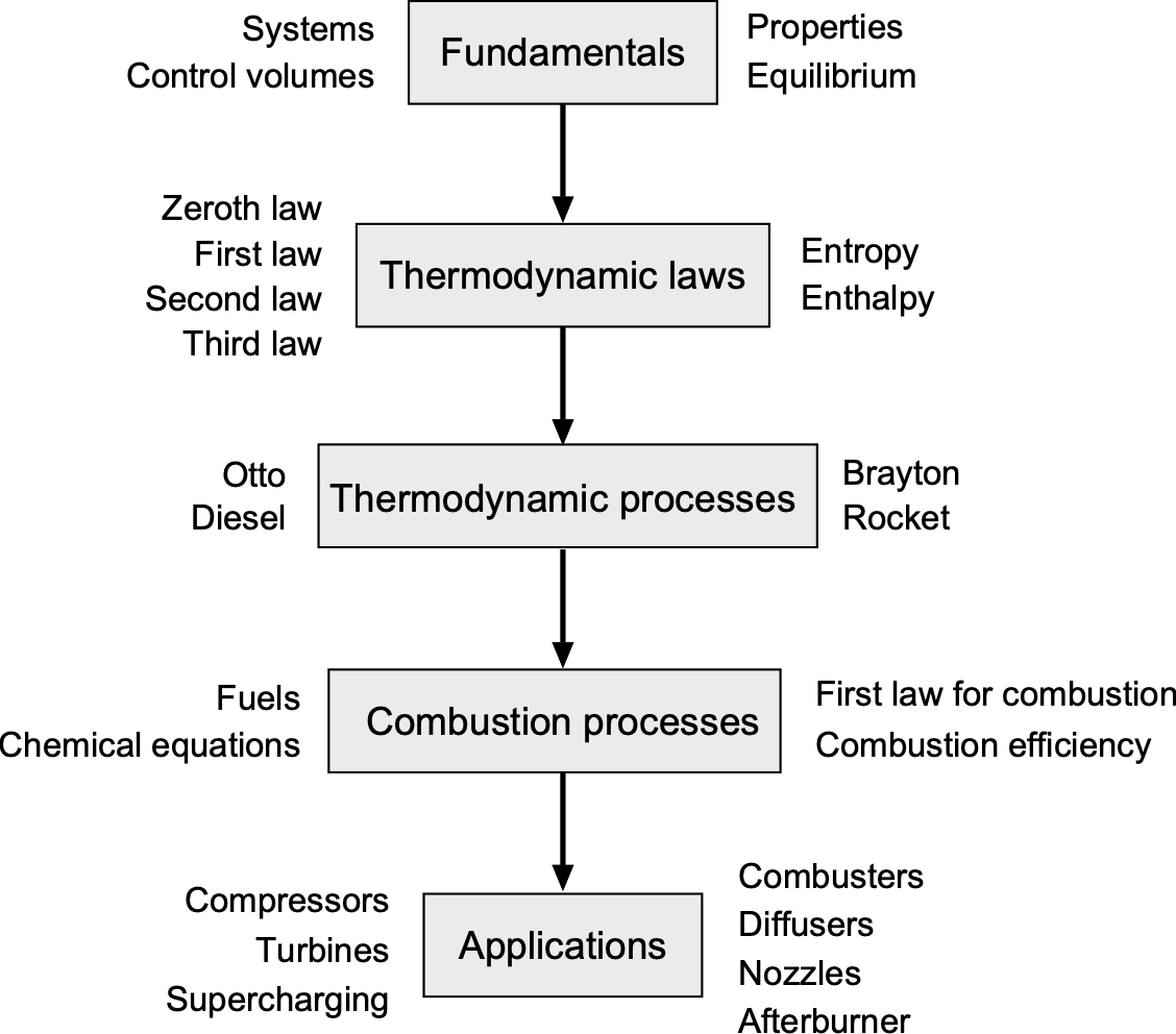
The Second Law of Thermodynamics follows, introducing the concept of entropy and establishing the limits on the reversibility and efficiency of processes. Alongside these principles, the equation of state and the ideal gas model provide the property relations that connect pressure, temperature, and density. With these tools in hand, the analysis extends to flow devices such as diffusers, compressors, turbines, combustors, and nozzles, which form the essential building blocks of propulsion systems. The chapter concludes with a brief exposition of combustion thermodynamics, where the conversion of chemical energy in fuels into thermal energy completes the framework for analyzing propulsion systems.
Fundamental Thermodynamic Concepts
Thermodynamics provides the principles for quantifying energy, work, and heat in engineering systems. In aerospace engineering, these principles extend beyond standard abstract definitions, as they provide a basis for analyzing propulsion cycles and flow processes in components such as diffusers, compressors, combustors, turbines, and nozzles. Every aerospace propulsion system, from a piston engine to a scramjet, is ultimately governed by the same fundamental laws of thermodynamics. To apply these laws, it is first necessary to define the basic concepts of systems, properties, and processes, which then naturally lead to the First Law of Thermodynamics, the principle of energy conservation that underpins all applications.
Measurable Quantities in Thermodynamics
A central feature of thermodynamics is its reliance on measurable macroscopic properties. These are quantities that can be directly determined with suitably calibrated instruments and then used to define the state of a system. The most fundamental properties are temperature, pressure, volume, and mass. Temperature is measured with devices such as thermocouples or various types of ordinary thermometers. Pressure is measured with manometers or electronic pressure transducers. The volume is obtained from geometric measurements of the system’s boundaries. From these, derived quantities such as density and specific volume follow immediately.
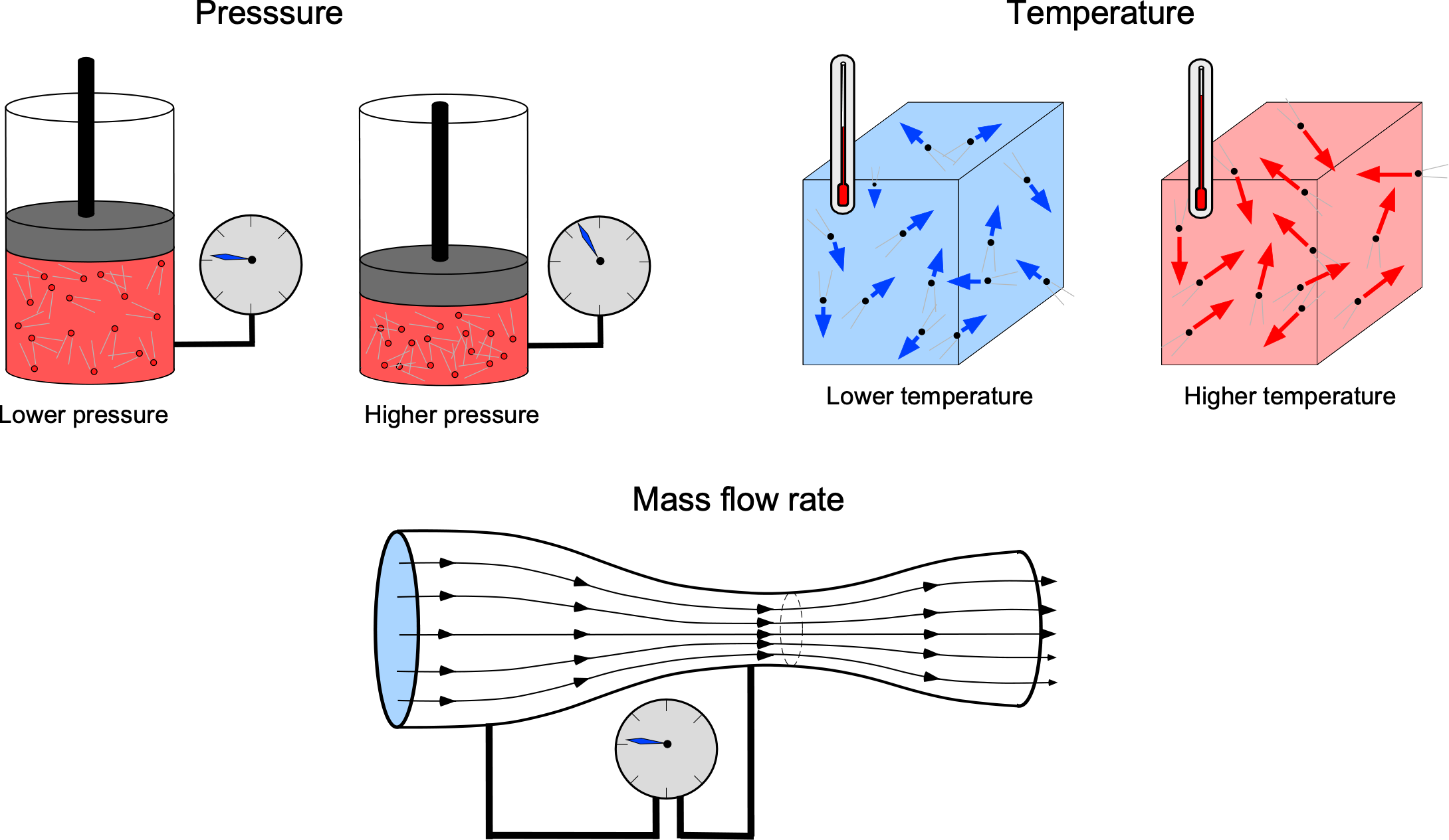
Other observable properties arise when processes occur. Flow rates of fluid mass or volume can be measured with nozzles, venturi meters, or flow sensors. Time is always measurable and plays a crucial role in transient processes where heating, cooling, or cycling rates are significant. Heat transfer and work interactions, though not properties that define a state, can also be quantified using experiments. Heat is measured indirectly, for example, using heat flux sensors, while work is obtained from integrals of pressure with respect to volume change, or mechanically by measuring the torque and rotational speed in engines and compressors.
Many of the quantities used in thermodynamics, however, are not directly measurable. Quantities such as internal energy, enthalpy, and entropy must be inferred from measurable properties using the First and Second Laws of thermodynamics together with the equation of state. Internal energy is defined only through its changes, often determined from calorimetric data, i.e., measured values that describe the heat associated with physical or chemical processes, such as temperature changes, phase transitions, or chemical reactions.
Enthalpy is obtained from internal and flow energy, which is based on measurable quantities, and represents the total energy content of a fluid available to do flow work. Entropy, as a property, is more abstract and is defined either through the ratio of heat transfer to temperature in a reversible process or by computing from property relations. Entropy is best understood as a measure of energy dispersion. Exergy, or availability, is a further thermodynamic construct that combines energy and entropy with the environment’s reference state to assess the potential for useful work. Exergy is the part of energy that is actually useful.
Therefore, the practice of thermodynamics rests on a hierarchy of concepts and principles: a foundation of directly measurable variables, a set of derived quantities that combine them, and a group of deeper concepts, such as energy and entropy, that must be inferred rather than measured. This distinction is crucial, for it explains why thermodynamics is rooted in observation and experimentation, with an overarching theoretical framework that connects those observations into general laws that can be used to predict thermodynamic and aerodynamic behaviors.
Systems and Control Volumes
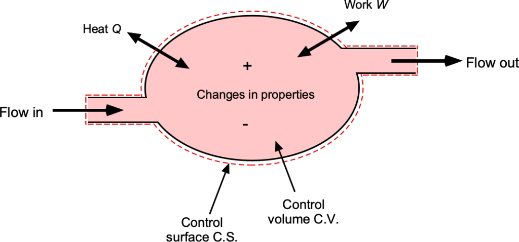
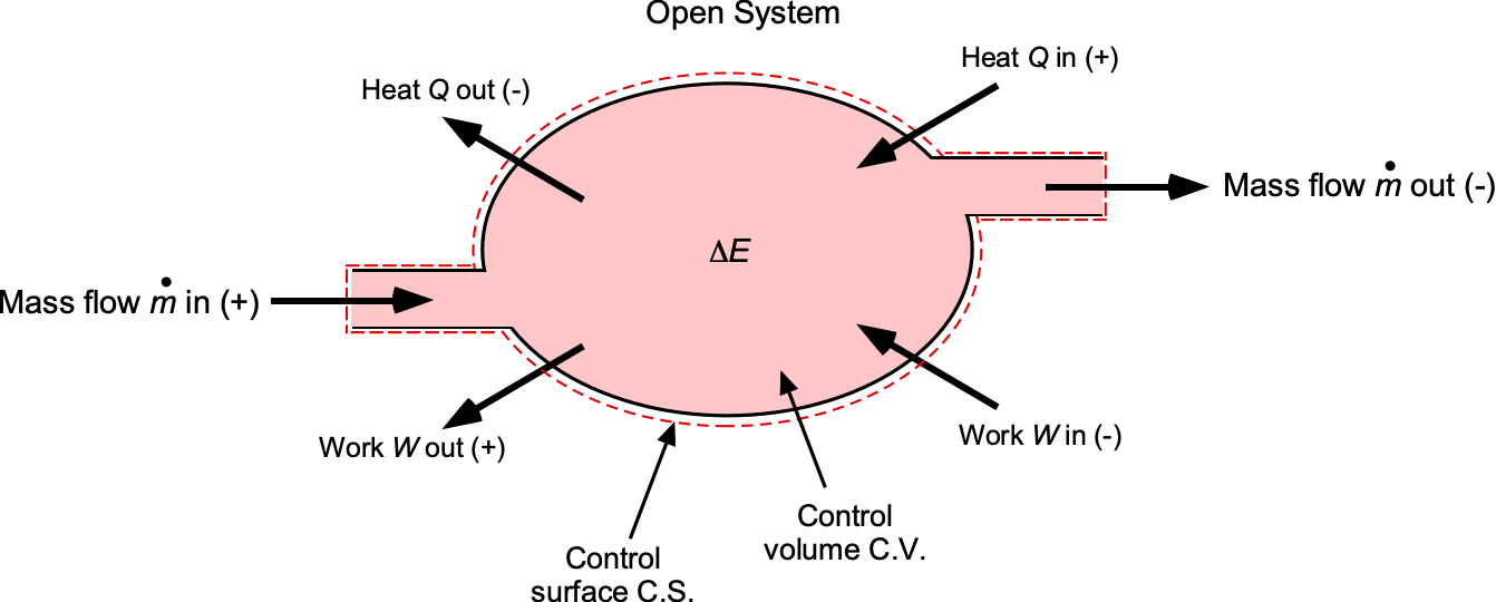
The first step in applying the principles of thermodynamics is to define the system of interest. A system is a fixed quantity of matter enclosed by a boundary, as shown in the figure below. Energy, in the form of heat or work, may cross this boundary, but the matter itself inside the system remains fixed. A control volume (C.V.) is defined as a specified region in space through which both mass and energy can cross over the control surface (C.S.). The use of control volumes and control surfaces is fundamental not only to thermodynamics but also to fluid dynamics and aerodynamics. The key to solving many engineering problems is the ability to define a suitable control volume in which to apply the physical laws.
Depending on how control volumes and boundaries are specified, different categories of systems can be obtained. In a closed system, mass does not cross the boundaries defined by the C.S., although energy transfer in the form of heat or work may still occur. An open system allows both mass and energy to cross the C.S., making it the most relevant model for aerodynamics and propulsion devices. An isolated system is an idealization in which neither mass nor energy can cross its boundary. While useful for theoretical developments and discussions, it has limited practical applications in aerospace contexts because they generally always involve mass flows into and out of a C.V.
For propulsion analysis, a C.V. is usually drawn to encompass a specific component such as a nozzle, compressor, turbine, or combustor. Inlet and outlet planes are selected at locations where the flow properties can be meaningfully averaged or measured, allowing the conservation of mass, momentum, and energy to be applied in a practical form. For example, when analyzing a turbojet combustor, a C.V. is defined around the burner chamber, with air and fuel streams entering and hot combustion products exiting. Multiple systems can be interconnected, with the output from one C.V. serving as the input to the next. This type of framework provides a consistent approach to applying the laws of thermodynamics, thereby linking fundamental principles to measurable net system performance.
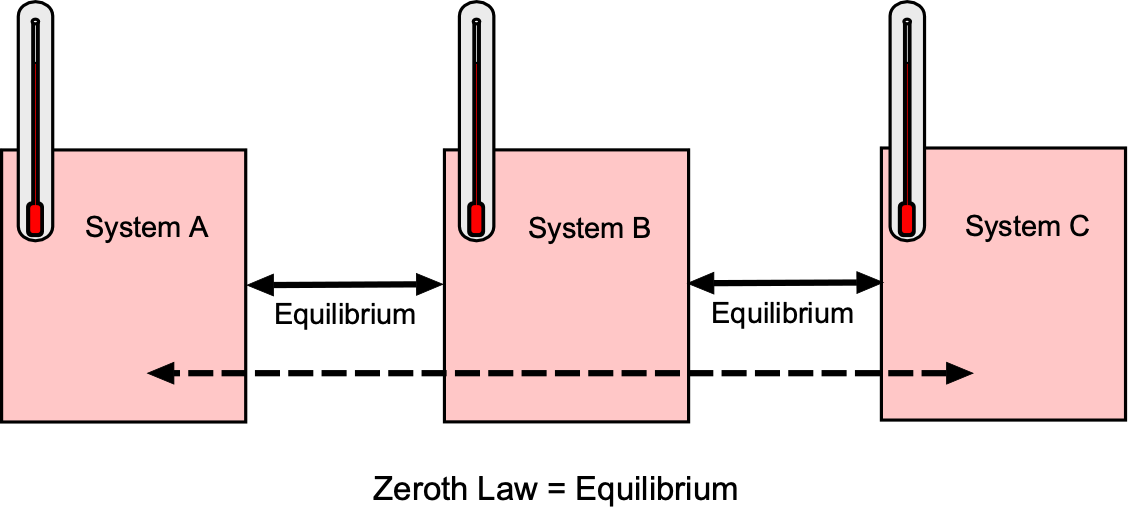
Zeroth Law of Thermodynamics
Many engineers are puzzled by the existence of the Zeroth Law of Thermodynamics. Although formulated after the First and Second Laws, the Zeroth Law was recognized in the 1930s as a more fundamental law because the “equilibrium transitivity” principle was so fundamental that it really should have been stated before the First Law. Because the numbering of the laws was already well established, it was given the name “Zeroth Law” to reflect its logical priority.
The Zeroth Law establishes the foundation for the concept of temperature. It states that if system A is in thermal equilibrium with system B, and system B is in thermal equilibrium with system C, then system A is also in thermal equilibrium with system C. In symbolic form, then
(1) 
as shown in the figure below. This transitive property[3] means there exists a single scalar property, i.e., the temperature  , that is equal for all systems in mutual thermal equilibrium. In practice, the Zeroth Law justifies the approach to temperature measurement using a thermometer. If a thermometer is brought into thermal contact with a system and no net heat flows at equilibrium, then the thermometer’s reading defines the system’s temperature.
In aerospace engineering, the Zeroth Law underpins all types of temperature sensing and calibrations. Engine test cells, wind tunnels, and flight instrumentation rely on sensors that must come to thermal equilibrium with the medium or surface of interest. Examples include thermocouples and resistance temperature detectors for combustor liners and turbine casings, as well as total-temperature probes used in engine inlets and wind tunnels.
Because the Zeroth Law is, in fact, an equilibrium statement, care is needed when interpreting measurements in fluid flows. A probe should be designed and installed so that, after sufficient time, the sensor and the fluid region of interest reach thermal equilibrium. Thermal equilibrium (i.e., no net heat flow between systems in contact) is not the same as a steady-state (i.e., properties unchanging in time). A sensor can sit in a steady flow yet still not be in thermal equilibrium with it if conduction, radiation, or mounting hardware biases the reading.
In high-speed flows, what is often desired is the stagnation (total) temperature. Total-temperature probes are engineered to equilibrate with the environment, minimizing extraneous effects, with any necessary corrections applied based on calibration. A general rule in temperature measurements and thermometry is always to allow time for equilibration before applying any necessary probe corrections.
Equation of State
All gases have measurable properties, including their pressure, temperature, and volume. Numerous scientific experiments and careful measurements have determined that these variables are quantifiably related. In this regard, there are four fundamental thermodynamic gas laws: Boyle’s Law, Charles’s Law, Gay-Lussac’s Law, and Avogadro’s Law. These are all empirical gas laws because their relationships were derived from laboratory experiments with gases. Boyle’s law states that for a constant mass, the volume of the gas is inversely proportional to its pressure, i.e.,
(2) 
where conditions 1 and 2 refer to the initial and final conditions, respectively. Charles’s law states that for a gas at a constant pressure, its volume is proportional to temperature, i.e.,
(3) 
Gay-Lussac’s law states that at a constant mass and volume, the pressure is proportional to temperature, i.e.,
(4) 
These three laws can be combined, leading to the combined gas law, which is written as
(5) 
Notice that Eq. 5 is a thermodynamic equation. The outcome is that, for a given mass of gas, if any two properties can be determined (i.e., measured or calculated), the combined gas law can be used to determine (i.e., calculate) the third.
Finally, Avogadro’s law states that the amount of a gas, usually in terms of moles, is proportional to its volume at constant pressure and temperature, i.e.,
(6) 
where  is the mass of the gas expressed in moles. Remember that 1 mole = 6.022
 10
10 atoms, which is called Avogadro’s number,[4]
  , so a mole (a base unit) can be used as a basis to measure the density of a gas.
These preceding relationships are formally embodied in an equation of state, which determines the quantitative relationships between a gas’s pressure, density (or mass and volume), and temperature. In physics and chemistry, students inevitably first come across the use of the general or universal equation of state for a gas, which is written as
(7) 
where  is called the universal gas constant, which is the same for all gases. The universal gas constant, , is related to the Boltzmann constant,
  , by
, by  .
.
However, this latter form of the equation of state is not particularly useful for engineering purposes, especially for finding and relating fluid properties at a point in space. But, if both sides of this general equation are divided by the mass of the gas, then the volume now becomes the specific volume,  , which is the reciprocal of the density of the gas. Recall that the “specific” in the term specific volume means “divided by mass,” i.e.,
(8) 
Therefore, an alternative but equivalent equation of state for a gas can be written as
(9) 
which is more commonly written as
(10) 
Equation 10 is the usual form of the equation of state used in engineering, gas dynamics, and aerodynamics. Notice also that this result is independent of the volume of the considered gas because it is expressed in terms of density, i.e., mass per unit volume. However, in this case, another (different) gas constant,  , must be used, which equals the universal gas constant in terms of moles divided by the gas’s mass per mole, i.e.,
(11) 
It will be apparent that the value of in Eq. 10 is not universal and depends on the gas, i.e., the value of the gas constant is specific to the gas. Subsequently, caution should be exercised to ensure that the correct value of is used in engineering calculations for each gas being considered, along with the proper units. A helpful table of the gas constants for some common gases is shown below. However, it is helpful to remember that all the forms of the equation of state are considered equivalent, i.e.,
(12) 
and which version to use depends, in part, on the problem being solved.
| Gas | Molecular weight  (kg kmol-1) (kg kmol-1) |
(J kg-1 K-1) |
(ft2 s-2 R-1) |
| Air | 28.97 | 287.0 | 211.5 |
| Oxygen | 31.999 | 259.8 | 191.7 |
| Nitrogen | 28.014 | 296.8 | 218.9 |
| Carbon dioxide | 44.010 | 188.9 | 139.2 |
| Hydrogen | 2.016 | 4,124.0 | 3,039.7 |
| Helium | 4.003 | 2,078.5 | 1,532.0 |
| Methane | 16.043 | 518.3 | 382.0 |
| Water vapor | 18.016 | 461.5 | 340.1 |
Because point properties are often desired in engineering problems with fluids, the most common form of the equation of state is
(13) 
If pressure and temperature are known, the density follows directly, i.e.,
(14) 
Therefore, the equation of state reduces the number of independent thermodynamic variables from three to two.
The relationships may also be visualized as a surface in three-dimensional  ,
,  , and space, where each point represents a unique equilibrium state, as shown in the figure below. For air under standard and moderate flight conditions, the ideal-gas model is an excellent approximation. Deviations will only occur at very high pressures or very low temperatures, where so-called “real-gas” effects become significant.
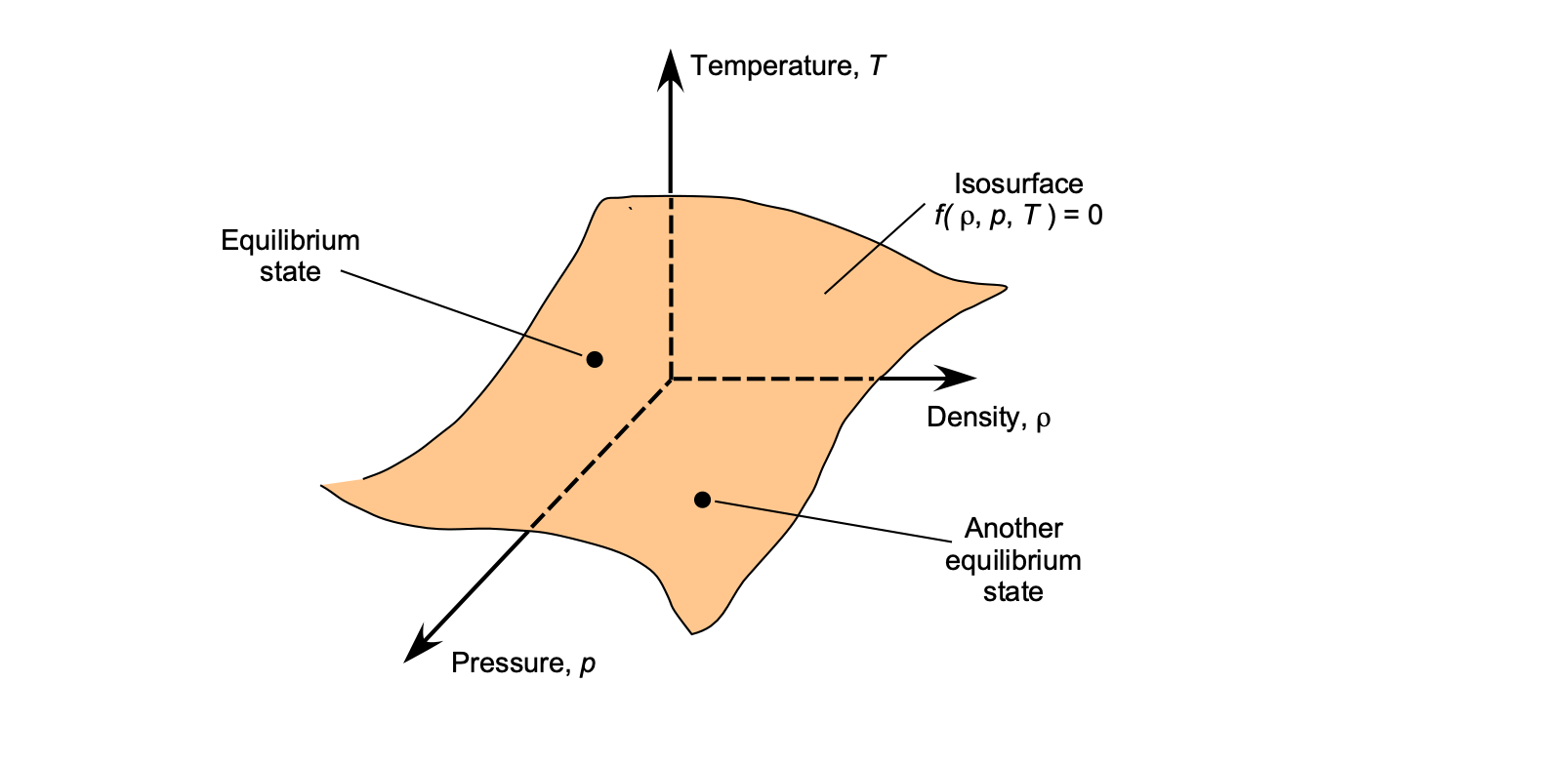 –– space; every point corresponds to a unique equilibrium thermodynamic state.
The ideal-gas model is generally valid for subsonic and supersonic propulsion analysis. Still, corrections are necessary at very high temperatures, such as in scramjet combustors or atmospheric re-entry flows, where real-gas effects (including dissociation and ionization) become increasingly critical. The study of high-speed, high-temperature gas flows is a specialized field in its own right, requiring descriptions based on chemical kinetics and statistical thermodynamics.
Units and Dimensional Consistency
More reminders about units are needed. Remember that both sets of units are aerospace engineering practice; SI units are standard in research, simulation, and most international collaborations, while USC units persist in many industrial applications and flight-testing contexts. As with other fields, thermodynamic expressions must be carefully applied with consistent units, most commonly the SI system. Dimensional homogeneity must always be checked so that every term in an equation represents the same physical dimensions. For example, the specific gas constant appears in the ideal gas law, i.e.,
![\[ p = \varrho \, R \, T \]](https://eaglepubs.erau.edu/app/uploads/quicklatex/quicklatex.com-f2b4ac456dbbe21201e05203eabe2c74_l3.svg "Rendered by QuickLaTeX.com")
where is pressure, is density, and is absolute temperature. From this relation, the dimensions of are
![\[ [R] = \frac{M\,L^{-1}\,T^{-2}}{M\,L^{-3}\,\Theta^{-1}} = L^{2}\,T^{-2}\,\Theta^{-1} \]](https://eaglepubs.erau.edu/app/uploads/quicklatex/quicklatex.com-2323030c5b433f175f633fe67f5d6093_l3.svg "Rendered by QuickLaTeX.com")
Therefore, in SI units, the units of are
![\[ [R] = \mathrm{J\,kg^{-1}\,K^{-1}} = \mathrm{m^{2}\,s^{-2}\,K^{-1}} \]](https://eaglepubs.erau.edu/app/uploads/quicklatex/quicklatex.com-fa407dfa1f3d22439a6f5c8ef0af04e4_l3.svg "Rendered by QuickLaTeX.com")
and in USC units
![\[ [R] = \mathrm{ft^{2}\,s^{-2}\,R^{-1}} \]](https://eaglepubs.erau.edu/app/uploads/quicklatex/quicklatex.com-b68d8122a7f1a1a0a63b335c67eda35a_l3.svg "Rendered by QuickLaTeX.com")
Heat & Work
Energy transfer to or from a system occurs in only two modes: heat and work. Heat is the mode of energy transfer that occurs solely because of a temperature difference between the system and its surroundings. Work is the mode of energy transfer, such as mechanical work, that occurs at the boundaries of the system. It should be understood that neither heat nor work is a property of an actual system, but transient interactions that appear only when energy crosses the system boundary.
Heat and work are process-dependent quantities that vanish when the system is isolated, i.e., heat and work cannot be stored within the system. However, properties such as temperature, pressure, internal energy, enthalpy, and entropy can be used to describe the thermodynamic state. Therefore, heat and work must be viewed as the sum of differentials  and
and  during a change from one state to another, i.e.,
(15) 
For example, consider a closed thermodynamic system containing a gas, as illustrated in the figure below. Its state in terms of pressure and temperature (and other properties) can be changed in different ways. In some processes, energy transfer occurs predominantly as heat, while in others, it occurs as work, and in most cases, it occurs as a combination of both.
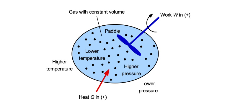
For example, heat could be added by conduction through direct contact with another body or by radiation from a combustion source, which will increase both the temperature and pressure. Work can be added by stirring the gas with a paddle or impeller, which will also change the pressure and temperature of the gas. The crucial point is that while the state of the system changes, the proportions of heat and work depend on how the process is carried out. There is an infinite variety of possible processes to change the state of the system, each involving a different combination of heat and work transfer.
Sign Conventions
To apply thermodynamic principles consistently, a sign convention must be clearly established. By classical thermodynamics convention, then  if heat is added to the system from the surroundings, and
  if the system does work on the surroundings. This choice of signs works well for both closed systems and open systems with fluid streams and mass flow rates, the latter being the most common type of system found in aerospace engineering.
This convention ensures consistent accounting of energy transfers across the components of an engine cycle. For example, in a jet engine, the compressor work input is considered negative, the turbine work output is positive, and their difference determines the net shaft power available. Similarly, in a rocket nozzle, there is no shaft work term; only internal energy changes and kinetic energy are relevant. The essential point is to maintain internal consistency when applying the equations of thermodynamics to solve practical problems.
The First Law of Thermodynamics
The First Law of Thermodynamics is the formal statement of the conservation of energy. It asserts that energy cannot be created or destroyed, but only transformed from one form to another, such as heat, work, and stored energy. For aerospace systems, this principle governs the conversion of fuel energy into useful thrust or shaft power.
The historical roots of this law can be traced back to the nineteenth century, when James Joule established the equivalence of heat and mechanical work. Rudolf Clausius later expressed this relationship in general mathematical form, laying the foundation for modern thermodynamics. In aerospace propulsion, the First Law provides the fundamental balance that connects compressors, turbines, nozzles, and combustors into a complete engine cycle.
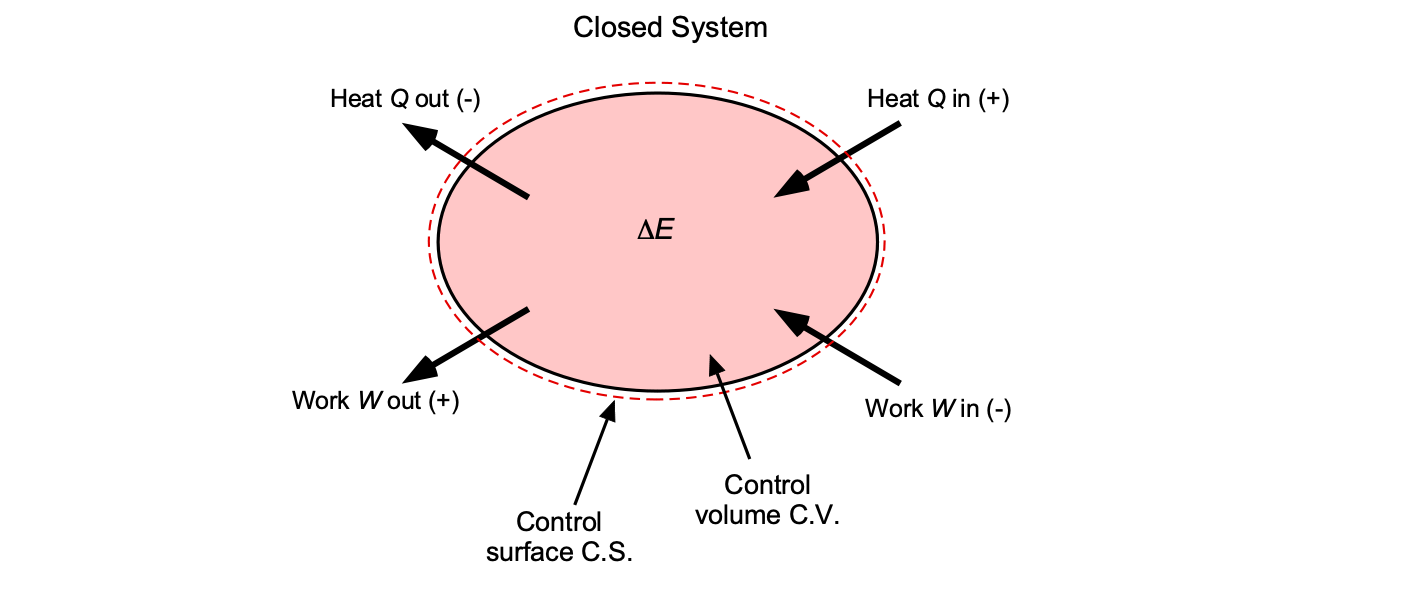
Closed System Form
For a fixed mass of matter (i.e., a closed system defined by a control volume (C.V.), as shown in the figure below), the First Law of Thermodynamics is expressed as
(16) 
where  is the net heat added to the system inside the C.V.,
  is the net work done by the system, and
  is the change in total energy of the system. By convention, heat added to the system is positive, and the work done by the system is negative.
The total energy of a system may be decomposed into three contributions, i.e.,
(17) 
where  is the internal energy,
  is the macroscopic kinetic energy, and
  is the corresponding gravitational potential energy. For most aerospace devices, the potential energy term is negligible compared to the internal and kinetic energy. Still, it must be retained for any system that undergoes significant changes in vertical height or altitude.
Open System Form
Most aerospace components are open systems where the mass flow enters and leaves the C.V., as shown in the figure below. For a fixed C.V., the First Law then becomes a power balance, i.e.,
(18) 
where  is the rate of heat transfer into the C.V.,
  is the net rate of work done by the C.V. (shaft work plus flow work), and
  is the specific energy, i.e.,
(19) 
For steady-flow operations, the storage term  , so the steady-flow energy equation becomes
(20) 
where  is the specific enthalpy, as defined by
(21) 
which is the sum of the specific internal energy and  is the specific flow work associated with pushing fluid mass into or out of the C.V. In propulsion devices, several simplifications are common, which include
  when neglecting elevation changes, and
  for adiabatic operations, as well as
  for no shaft work, e.g., a nozzle.
The specific flow work needs some further discussion. Imagine a steady stream of fluid entering a C.V. over an area  , with velocity
  , pressure , and density . The pressure force acting on is
  . During a time interval
  , a slug of fluid of length
  enters, with a fluid volume of
  . The work done by the pressure force to push this slug into the C.V. is
(22) 
Dividing by the mass of the slug,  , gives the specific flow work term as
(23) 
This derivation shows that the so-called specific flow work is nothing more than the work done by pressure forces expressed in terms of per unit mass of the flowing fluid. The term  appears automatically when a control volume is used.
For this reason, it is convenient to combine the internal energy  per unit mass with the specific flow work term
  to form the specific enthalpy, i.e.,
  . Enthalpy, therefore, arises naturally in the First Law of Thermodynamics for open systems, ensuring that both the internal energy carried by the fluid and the ability to extract or do work are accounted for in a single property.
It should be emphasized that enthalpy is not a new form of energy, but simply a convenient grouping of internal energy and the energy to do flow work. Like all specific energy terms, enthalpy has units of energy per unit mass (in SI units, then J/kg, which are dimensionally equivalent to m /s), the same as the kinetic and potential energy terms per unit mass. Its usefulness is mainly bookkeeping, i.e., instead of tracking and separately, enthalpy combines them into a single property.
Notice that in the USC system, energy is usually expressed in foot-pounds force (ft-lb), where 1 ft-lb = 1.356 J. Thermal energy is sometimes given in British thermal units (BTU), with 1 BTU = 778 ft-lb = 1,055 J. However, a BTU is now a depreciated unit in most branches of engineering.
Differential Form
For an infinitesimal process in a closed system, the First Law may be written in differential form as
(24) 
where  and
and  represent the path-dependent heat and work transfers, while , , and
  are state functions representing the internal, kinetic, and potential energies of the system. Dividing through by the system mass
  gives the per-unit-mass form, i.e.,
(25) 
where  is the specific internal energy, and
  and
and  denote the heat and work transfers per unit mass.
For a finite change between two states, integration gives
(26) 
which is the form most often used in aerospace applications, where energy transfers are naturally considered on a per-unit-mass or per-unit-mass-flow basis, i.e., in terms of the local density of the flow.
For an infinitesimal process in an open system with steady flow into and out of a C.V., the First Law may be expressed as
(27) 
where  and
and  are the rates of heat and work transfer across the control surface, and
  is the mass flow rate. Again, notice the occurrence of the enthalpy , which combines the internal energy with the specific flow work
  . On a per-unit-mass basis, this reduces to
(28) 
where  and
and  are the heat and work transfers per unit mass of flow.
This is called the steady-flow energy equation (SFEE) and is the most widely applied form of the First Law in aerospace applications. It shows that the heat and work interactions with a flow process must equal the combined changes in enthalpy, kinetic energy, and potential energy between the inlet and the outlet. For many propulsion components, the potential energy term is negligible, while kinetic energy changes dominate in nozzles and diffusers, and enthalpy changes dominate in compressors and turbines.
Remember that the sign conventions previously discussed should be used to ensure consistency when applying the First Law of Thermodynamics across the interconnected components of propulsion and power cycles.
Special Cases in Aerospace Devices
The reductions of the First Law above illustrate how the general energy equation simplifies when applied to individual components of an aerospace propulsion system. By invoking the First Law under suitable assumptions, simplified working equations can be obtained for standard devices. For example, in a nozzle, the flow can be considered adiabatic, with negligible shaft work and heat transfer. The stagnation enthalpy remains constant, i.e.,
(29) 
so any increase in velocity is accompanied by a corresponding decrease in static enthalpy. The nozzle efficiency is defined by
(30) 
In a compressor, heat transfer and changes in potential energy are negligible. The principal energy interaction is the shaft work input per unit mass, which is given approximately by
(31) 
with an isentropic efficiency of
(32) 
Here  is the enthalpy at the end of an ideal isentropic compression from state 1.
In a turbine, the situation is reversed, i.e., work is extracted from the fluid. For an adiabatic turbine, the shaft work per unit mass flow is
(33) 
with an isentropic efficiency of
(34) 
Finally, in a combustor, there is no shaft work, and the effect to consider is the addition of heat. The primary consequence is an increase in the enthalpy of the working fluid resulting from the release of chemical energy from the fuel, i.e.,
(35) 
with a combustion efficiency of
(36) 
Here,  is the fuel-air ratio, and LHV denotes the lower heating value of the fuel, which measures the chemical energy released when the fuel burns completely with the water vapor remaining in the exhaust. This convention is standard in aerospace propulsion because turbines and rocket engines do not recover any of the latent heat of vaporization.
Nozzles & Diffusers
In a nozzle, as shown in the figure below for a subsonic flow, there is no shaft work ( ), so the process is a conversion between pressure energy and kinetic energy. However, the behavior of pressure and velocity is opposite in subsonic and supersonic flow. For subsonic flow (
 ), the pressure decreases (
 ), the velocity increases (
 ), and the static temperature decreases slightly (
 ).
).
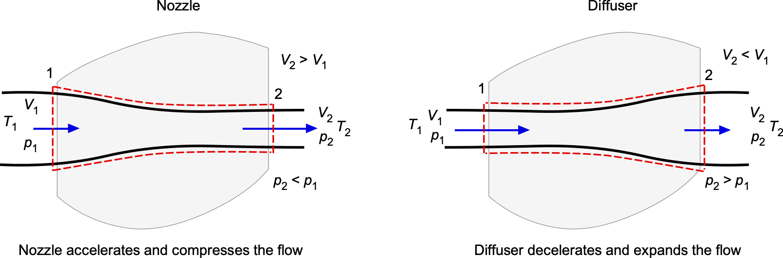
For supersonic flow ( ), the relations reverse in a converging passage, i.e., the pressure rises (
 ) while the velocity decreases (
 ), with a corresponding rise in static temperature (
 ). A diffuser shows the same complementary trends. In subsonic flow, and , while in supersonic flow, and , usually resulting in a significant pressure drop and an increase in velocity, as seen in the exhausts of rockets and jet engines. In all cases, the static temperature changes with the pressure changes, but the stagnation temperature,
  , remains nearly constant if the process is adiabatic.
Stagnation Temperature
In a compressible fluid flow, it is important to distinguish between the static temperature of the moving fluid and the stagnation temperature  . The static temperature represents the molecular kinetic energy associated with random thermal motion, as would be measured by a thermometer moving with the fluid. The stagnation temperature, by contrast, is defined as the temperature the fluid would reach if it were decelerated to zero velocity in an isentropic manner. For a perfect gas, this relation is
(37) 
where is the Mach number of the flow, and  is the ratio of specific heats. For low Mach numbers, the static and total temperatures are identical.
The use of stagnation temperature, therefore, accounts for both the thermal energy of the fluid and the kinetic energy associated with its bulk motion. In an adiabatic process with no shaft work, the total energy of the fluid is conserved. The static temperature will vary as the flow is compressed or expanded because of pressure and density changes, but the stagnation temperature remains nearly constant.
For example, when a flow is compressed adiabatically in a nozzle or a diffuser, the static temperature rises as kinetic energy is converted into internal energy. In contrast, the stagnation temperature remains constant. Similarly, in an adiabatic expansion, the static temperature decreases, but again, the value of remains constant.
This invariance of stagnation temperature in adiabatic flow is a direct consequence of the First Law of Thermodynamics. Only if there is heat transfer to or from the flow, or if shaft work is extracted, will the stagnation temperature change. For this reason, serves as a convenient reference value in propulsion analysis in that it provides a measure of the total energy content of a fluid stream. This energy is conserved through adiabatic machines such as compressors, turbines, and nozzles, even though the local static temperature and other flow properties may vary considerably.
Compressors & Turbines
Compressors and turbines, as illustrated in the schematic below, are utilized in various engineering applications. They involve shaft work transfer in addition to pressure changes. In aerospace engineering practice, the following systems and conventions are used:
- Compressor or pump: Shaft work is negative because energy is added to the fluid.
- Turbine: Work is positive because energy is extracted from the fluid, e.g., to drive a shaft.
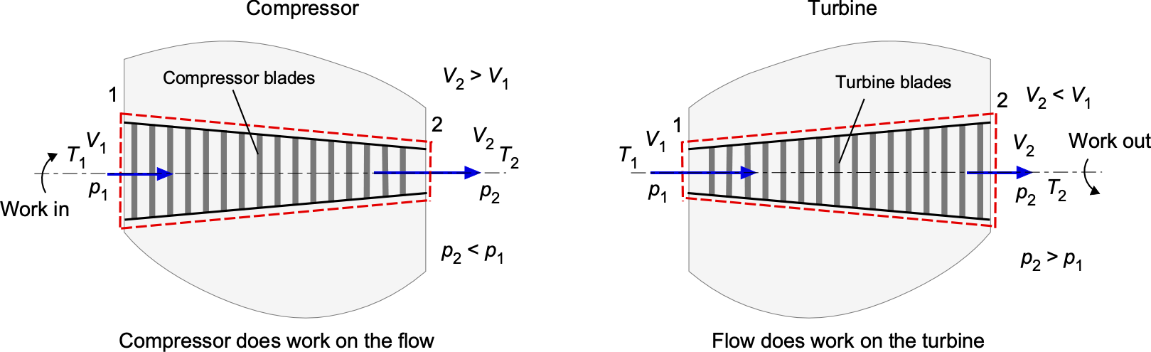
In a compressor, the application of shaft work increases the pressure of the fluid, resulting in  and
and  . The velocity change in the flow is usually modest because the compressor’s role is to raise the stagnation pressure, not the flow velocity. In a turbine, shaft work is extracted, so
  and
and  . The flow velocity may increase or decrease depending on the blade design; however, the dominant effects are a decrease in pressure and temperature across the stage.
These inlet-outlet relations also reinforce the sign conventions for work transfer. Compressors require shaft work input, and turbines deliver shaft work output. The trends in  ,
,  , and
, and  depend strongly on whether the flow is subsonic or supersonic, and this distinction turns out to be crucial for all forms of propulsion analysis.
In compressors, the relative Mach number through the blade passages is kept subsonic because any occurrence of shock waves would cause significant entropy increases (losses), flow separation, and a smaller pressure rise, leading to a loss of efficiency. Although small supersonic pockets may still occur near the blade tips, compressor design principles ensure that overall the stage remains subsonic in the rotating frame. For this reason, decelerating high-speed inflow to subsonic conditions requires a suitable inlet system placed ahead of the compressor, which may involve the use of diffusers, ramps, or inlet guide vanes.
Turbines, however, can and often do operate with supersonic expansions, particularly in the nozzle guide vanes where the hot gases are accelerated. Controlled supersonic flow is acceptable provided the resulting shock waves and expansions are appropriately managed. However, uncontrolled supersonic relative inflow to the turbine stages causes efficiency losses. Therefore, while compressors are essentially subsonic devices, turbines may contain both subsonic and supersonic regions depending on the stage design and its operating conditions.
Properties, State, & Equilibrium
A property is a measurable characteristic of a system, such as pressure or temperature. Thermodynamics classifies properties in ways that help engineers distinguish between those inherent to the material and those that depend on the system’s scale. Intensive properties, including pressure , temperature , and density , do not depend on the amount of matter present. In contrast, extensive properties such as mass , total volume  , and total energy
  scale with the size of the system. Therefore, to compare systems of different sizes, it is often convenient to define specific properties on a per-unit-mass basis, e.g.,
(38) 
where is the specific volume and is the specific energy.
The complete set of property values at a given instant defines the state of a system. A system is said to be in thermodynamic equilibrium when no unbalanced driving conditions exist. Mechanical equilibrium corresponds to uniform pressure with no net forces, thermal equilibrium requires a uniform temperature field, and chemical equilibrium implies that no net reactions are taking place.
Processes & Paths
A process in thermodynamics refers to a change of state of a system, while the ordered sequence of intermediate states through which the system passes is referred to as the path. This distinction is fundamental in thermodynamics. State functions (or properties) depend only on the initial and final states, regardless of the path. Examples include internal energy , enthalpy  , entropy
  , and pressure . For a state function
  , the change is written as
(39) 
which makes clear that state functions are exact differentials, i.e.,  ,
,  and
and  .
.
Path functions, in contrast, depend on the manner in which the process is carried out. Heat transfer, , and work, , are typical examples. They are expressed as inexact differentials, i.e., and to emphasize their dependence on the process rather than the state. Because of this, for a closed system, the First Law of thermodynamics is written as
(40) 
where is an exact differential (a state function), but and are inexact differentials (path functions).
This distinction means that the same change in a state function (for example,  ) can be achieved by an infinite number of different paths, each involving different amounts of heat and work, i.e., in general
(41) 
In propulsion analysis, idealized processes such as isentropic compression in a compressor or isentropic expansion in a turbine serve as baselines. The deviations of real devices from these idealized paths provide a direct measure of their efficiency. Therefore, while the changes in , , and  are dictated solely by the end states, the actual heat and work transfers, and consequently the performance of real engineering devices, depend on the precise thermodynamic path that is followed.
The distinction between state functions and path functions can be better explained by considering a – diagram. The figure below shows two thermodynamic paths, A and B, that connect the same initial and final states. Regardless of the chosen path, the changes in state functions such as internal energy , enthalpy , and entropy depend only on the initial and final conditions. However, the heat and work exchanged with the surroundings are path functions, and therefore take on different values along Path A compared with Path B.
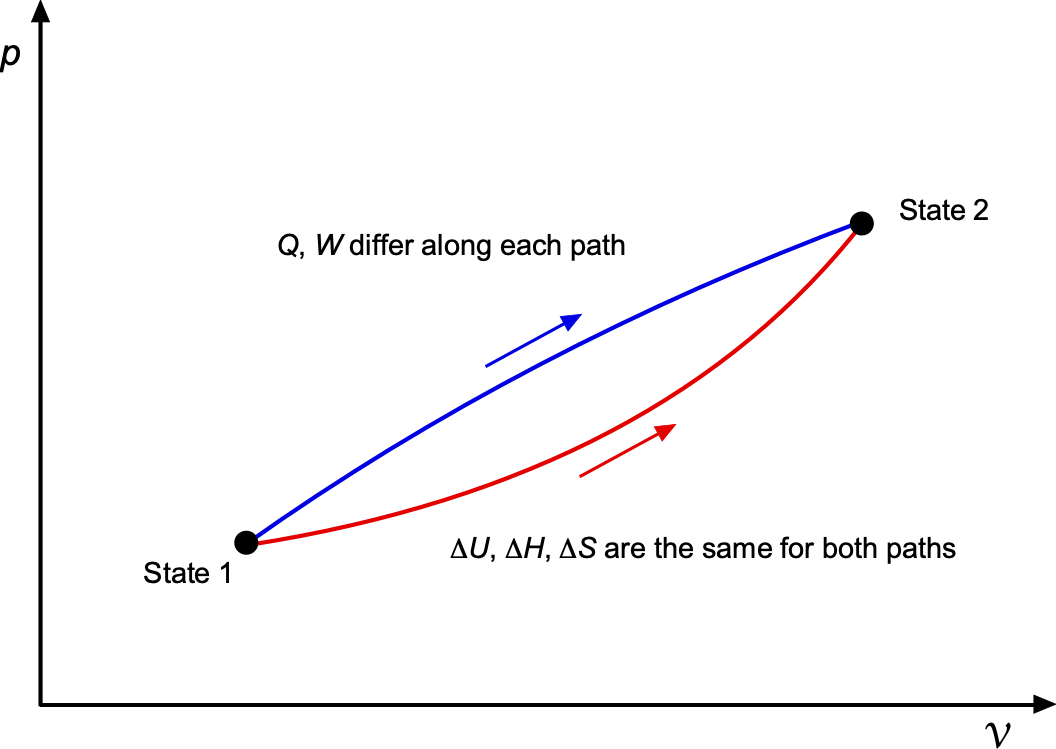 – diagram.
This example illustrates why the change in internal energy, i.e.,  is uniquely defined by the states, whereas and are process-dependent quantities, i.e.,
  .
.
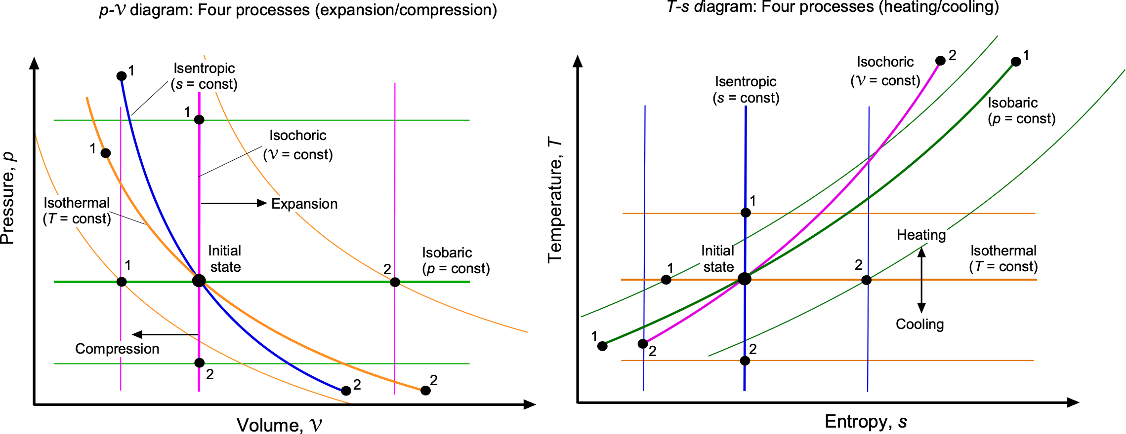
Property Diagrams
Thermodynamic processes and cycles are most clearly understood with the aid of property diagrams, which provide a visual depiction of how energy is stored, transferred, and degraded. The two most important are the pressure-volume or  diagram as previously described, and the temperature-entropy or
  diagram. Taken together, they form the foundation for interpreting both idealized and practical engineering processes.
On a diagram, the emphasis is on work interactions. The area under any one process curve represents boundary work, while the area enclosed by a cycle corresponds to the net work output or input. On a diagram, the emphasis shifts to heat transfer and irreversibility. The area under any one process curve represents the heat transfer, and the area enclosed by a cycle quantifies the combined balance of work and heat. Because entropy change measures irreversibility, deviations from any isentropic paths immediately reveal efficiency losses. In aerospace applications, diagrams are particularly valuable in analyzing propulsion systems because temperature and entropy changes across compressors, combustors, turbines, and nozzles determine both efficiency and design limits.
The characteristic features of the standard idealized processes are shown in the figure below. On the diagram, an isobaric (constant pressure) process appears as a horizontal line, while an isochoric (constant volume) process appears as a vertical line. Lines of constant temperature (isotherms) are hyperbolic curves determined by  constant. Isentropic compression and expansion processes follow lines of
  constant.
On the – diagram, an isobaric process appears as a positively sloped curve given by
  , while an isochoric process appears as a curve of different gradient,
  . An isothermal process is a horizontal line (
 constant), and an isentropic process is a vertical line (
 constant). These features give immediate visual insight into the physics of each thermodynamic process.
Better Understanding Entropy
A better understanding of entropy can be gained by relating its definition to the physical behavior of systems. Entropy measures how energy is dispersed among the possible microscopic states of a fluid. When heat is added at a high temperature, the entropy change is relatively small because the energy is absorbed into already excited states. When the same heat is added at a low temperature, the entropy change is larger because many more states become accessible. This is why entropy is defined in differential form as
(42) 
For ideal gases with constant specific heats, the entropy change takes the form
(43) ![\begin{align*} \text{Isothermal:} \quad & \Delta s = \frac{q_{\text{rev}}}{T} \\[5pt] \text{Isochoric:} \quad & \Delta s = c_v \ln\!\left(\frac{T_2}{T_1}\right) \\[5pt] \text{Isobaric:} \quad & \Delta s = c_p \ln\!\left(\frac{T_2}{T_1}\right) \\[5pt] \text{Isentropic:} \quad & \Delta s = 0 \end{align*}](https://eaglepubs.erau.edu/app/uploads/quicklatex/quicklatex.com-9cd26ddf4244117aa329e436203462c5_l3.svg "Rendered by QuickLaTeX.com")
More generally, for an ideal gas undergoing any process between states 1 and 2, the entropy change can be expressed as
(44) 
or equivalently as
(45) 
where is the gas constant (gas specific). On the diagram, entropy serves as a natural coordinate for visualizing thermodynamic cycles. The area under a process curve represents the heat transfer, i.e.,
(46) 
which makes the diagram a powerful tool for interpreting thermodynamic processes and cycles.
Gibbs Thermodynamic Surface
Josiah Gibbs recognized that all equilibrium properties of a simple substance can be represented as a single surface relating internal energy, entropy, and volume. This surface, known as the Gibbs thermodynamic surface, provides a unified picture of the relationships among the state variables , , , , and . For a simple compressible substance, the total differential of the internal energy is
(47) 
This is sometimes called the Gibbs equation. It combines the first and second laws of thermodynamics into a single expression. On the three-dimensional surface  , the temperature and pressure appear as the slopes
(48) 
Each point on the surface represents an equilibrium state of the system, and the tangent plane at any point gives the local values of and , as shown in the figure below. The and diagrams are two-dimensional forms of this more general surface. Gibbs’s geometric view therefore unifies the property diagrams and provides a visual link between thermodynamic quantities.
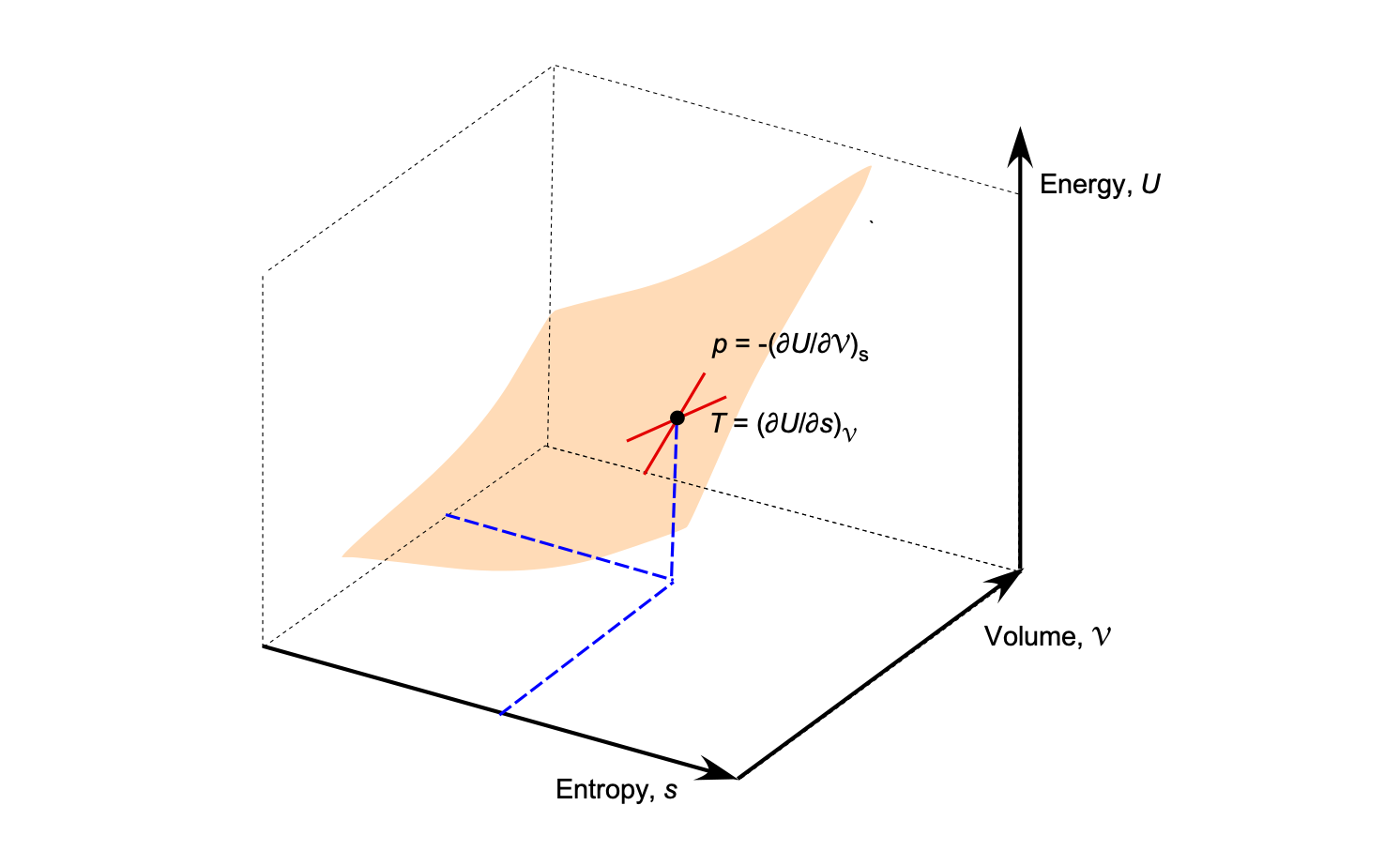 , where each point on the surface corresponds to an equilibrium state.
This differential form in Eq. 47 is used to evaluate energy and work interactions for processes in closed systems, such as piston-cylinder arrangements. For such systems, the elementary work is  and the elementary heat is
  , both of which follow directly from the Gibbs relation in Eq. 47. Therefore, the Gibbs surface provides a geometric link between the familiar – and diagrams and the underlying thermodynamic laws.
Piston-Cylinder System
To further understand the values of such process diagrams, a piston-cylinder system provides a useful physical and tangible model to illustrate how these processes may arise in practice, e.g., in a machine. As shown in the figure below, a frictionless, movable piston confines a fixed mass of gas. By adding or removing heat or allowing the piston to move, the state of the system can be altered. The corresponding piston motions and energy exchanges involve internal energy, heat flow, and work transfer, partly as a result of the piston’s movement.
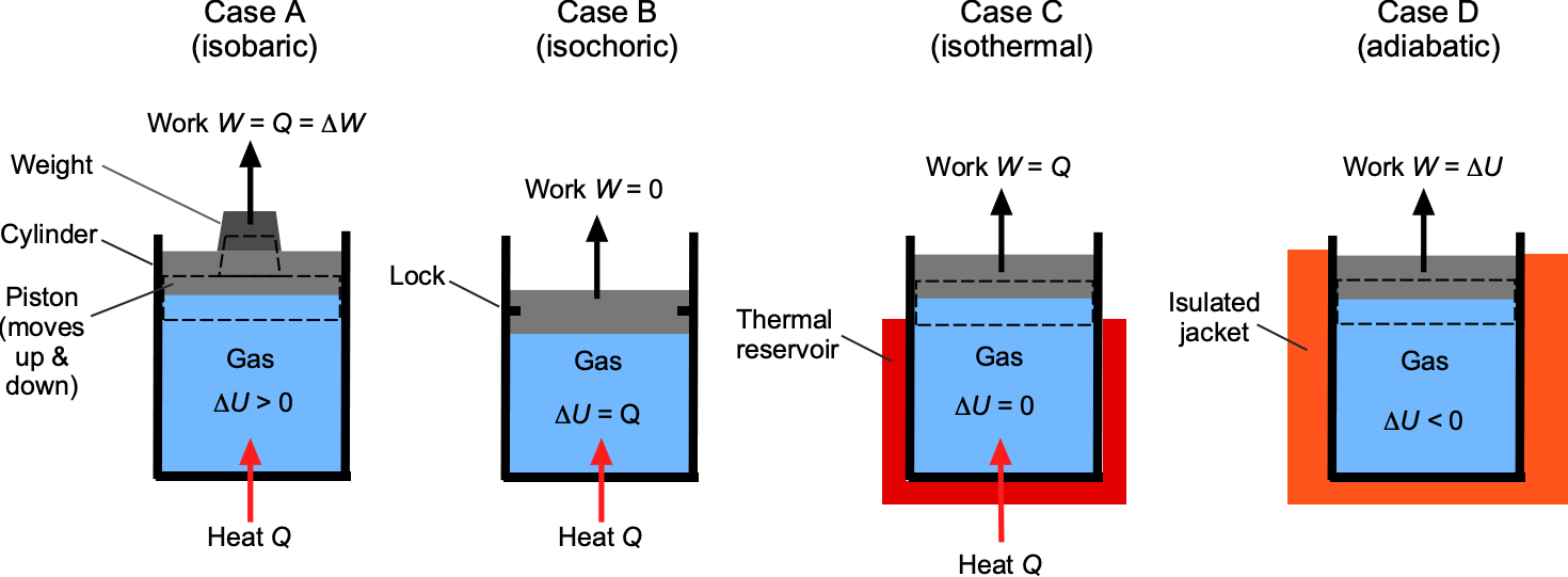
Consider first an isobaric process, in which the piston moves upward or downward while maintaining constant pressure, which is Case A. This condition can be simulated by placing a weight on top of the piston, thereby maintaining the pressure level in the trapped gas. On the diagram, this process appears as a horizontal line, and the work done is  . Because the temperature of the gas changes, its internal energy also changes, so that . On the diagram, the same process appears as an increasing or decreasing curve, depending on whether external heat is being added or removed.
If the piston is locked so it cannot move, as in Case B, the process is isochoric, and the volume remains fixed. No work is done ( ), so any heat transfer only alters the internal energy of the gas. On the diagram, this process appears as a vertical line; on the diagram, it appears as a curve whose slope reflects the change in entropy with temperature.
In an isothermal process, as in Case C, the system is placed in contact with a thermal reservoir, ensuring the temperature of the gas remains constant. For an ideal gas, the internal energy depends only on temperature, so  and the heat transfer equals the work, i.e.,
  . On a diagram, the path is a form of hyperbolic curve, while on the diagram it is a horizontal line.
Finally, an adiabatic process (Case D) occurs when no heat crosses the boundary, either because the cylinder is perfectly insulated or because the process takes place so rapidly that there is no time for any heat exchange. In this case, work is entirely at the expense of internal energy, so an expansion lowers the temperature, while compression raises it. On a diagram, the path is steeper than for an isothermal process, and on a diagram, it is vertical if the process is reversible, i.e., isentropic.
Specific Heats
The specific heats of a substance are terms frequently used in thermodynamics; they help measure how much its internal energy or enthalpy changes with temperature. They provide the link between temperature changes (which can be measured) and changes in stored energy (which cannot be measured directly).
Specific heats are always defined with respect to a constraint, because the way energy is partitioned between internal energy and expansion work depends on the conditions of the process. Formally, the specific heat at constant volume is defined as
(49) 
which represents the energy required to raise the temperature of a unit mass of gas by one degree while keeping its volume fixed. Under this condition, no boundary work is done, so all of the energy supplied goes into raising the internal energy of the gas.
The corresponding specific heat at constant pressure is defined as
(50) 
which represents the energy required to raise the temperature of a unit mass of gas by one degree while keeping the pressure fixed. At constant pressure, the volume expands as temperature increases, so part of the energy supplied is used as boundary work  , and the remainder increases the internal energy. As a consequence, the numerical value of
  is always greater than
  for gases.
For a perfect gas, there are simple and useful relationships among the values of the specific heats, the specific gas constant , and the ratio of specific heats , which are
(51) 
These relations are exact for an ideal gas and only approximate for real gases over moderate temperature ranges. The ratio is critical in aerospace applications because it enters directly into the compressible flow equations and the determination of the speed of sound,  , i.e.,
(52) 
The specific heats have SI units of J kg K (equivalently N m kg K). In USC units, they are expressed as ft-lb, slug R, with the unit ft-lb being the unit of work. Notice that the magnitudes of the specific heats will also depend on the molecular structure of the gas. Monatomic gases (such as helium) have lower specific heats than diatomic gases (such as nitrogen, oxygen, and air), which in turn differ from polyatomic gases. These differences reflect the number of molecular degrees of freedom (translation, rotation, and vibration) available for energy storage.
In aerospace engineering practice, specific heats are central to the energy accounting in all types of air-breathing propulsion devices. For example, the work input to a compressor is proportional to the change in enthalpy  . Additionally, the work extracted in a turbine is directly proportional to the drop in enthalpy, as previously discussed, and the jet velocity from a nozzle can be expressed in terms of enthalpy changes.
Representative Thermodynamic Properties of Dry Air
For dry air near standard conditions ( 300 K), the following tabulated values are commonly used in thermodynamic calculations. They are more often than not treated as constants, i.e., a calorically perfect gas. In reality, and increase gradually with temperature, especially above about 600 K, a behavior that becomes relevant in combustion and high-speed flight. For rockets and high-temperature gas flows (e.g., hypersonics), more accurate values of as a function of temperature must be used, which are obtained from property tables or curve fits to measured data.
| Property | SI Units | Value (SI) | USC Units | Value (USC) |
| Specific heat at constant pressure, |
J kg-1 K-1 |  |
ft-lb slug-1 R-1 |  |
| Specific heat at constant volume, |
J kg-1 K-1 |  |
ft-lb slug-1 R-1 |  |
| Gas constant, |
J kg-1 K-1 |  |
ft-lb slug-1 R-1 |  |
Ratio of specific heats,  |
— | 1.4 | — | 1.4 |
| Molar mass of air, |
kg mol-1 |  |
lb lb mol-1 |  |
| Speed of sound at 300 K, |
m s-1 |  |
ft s-1 |  |
Phase Changes
Air can usually be treated as a single-phase, calorically perfect gas in most aerodynamic applications. When moisture is present, however, the thermodynamic state of the air may depart from the ideal-gas behavior if the flow experiences a rapid pressure drop or if liquid water is present on a surface. In such cases, the local static temperature can fall to the saturation temperature of the water vapor in the air, allowing condensation to occur.
A useful starting point is the isentropic relation for a perfect gas undergoing a rapid expansion, i.e.,
(53) 
where is the static temperature, is the static pressure, and is the ratio of specific heats. If the air initially contains water vapor, the vapor partial pressure at the initial state is
(54) 
where  is the vapor partial pressure,
  is the initial relative humidity, and
  is the saturation vapor pressure at temperature
  . Before any condensation occurs, the vapor partial pressure scales with the total pressure, i.e.,
(55) 
Condensation begins at the first state  for which
(56) 
where  is the saturation vapor pressure at temperature . An approximate expression for the temperature dependence of the saturation vapor pressure follows from the Clausius-Clapeyron relation, i.e.,
(57) 
where  is the latent heat of vaporization and
  is the gas constant for water vapor. Equations 53 to 56, therefore, provide a simple way to check whether a rapid expansion will reduce the temperature below saturation and produce condensation. Once condensation begins, the release of latent heat partly offsets the temperature drop predicted by the dry isentropic relation.
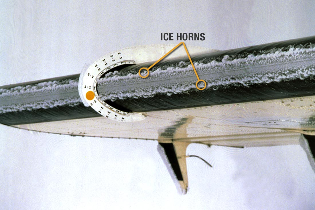
Several practical examples illustrate where a phase change is noticeable from thermodynamic means. The condensation clouds that form around an aircraft, flying at transonic or supersonic speeds, as shown in the photograph below, where rapid expansion lowers the static temperature below the saturation temperature or dew point. Helicopter rotors and propeller blades can show similar effects in humid air, producing spiraling condensation trails as the pressure drops in the tip vortices.
Phase change also affects surface temperatures when liquid water forms on the surface or is carried onto it. A wetted surface in an airstream satisfies an energy balance of the form
(58) 
where  is the recovery temperature,
  is the wall temperature, and
  are the heat and mass transfer coefficients, and
  and
and  are the saturation and freestream vapor densities. The latent-heat term explains why a wet surface can be much cooler than the adiabatic wall temperature. In icing conditions, the freezing of supercooled droplets adds another latent-heat term, but such cases are normally treated in dedicated icing analyses.
Evaporative cooling becomes evident when an aircraft flies through rain or cloud layers, often producing surface temperatures that are lower than those predicted by adiabatic relations. Under these conditions, ice may form on the leading edges of wings (see the photograph below) and on other exposed surfaces such as engine intakes, propeller blades, and sensor probes. Even a thin layer of ice can change the local geometry, increase drag, and dangerously increase the stall speed. As ice accumulates, the boundary layer can separate earlier, and stall margins can decrease. Ice accretion inside engine inlets can disrupt the airflow entering the compressor, potentially leading to a loss of thrust or compressor stall. These effects occur because freezing alters both the surface temperature and the behavior of the boundary layer, illustrating how moisture can modify the local thermodynamic conditions of the flow.
Internal Energy
Internal energy is the energy associated with the microscopic motions and interactions of the molecules in a fluid. The total internal energy is denoted by , and the specific internal energy by . For an ideal (perfect) gas, the specific internal energy depends only on temperature, i.e.,  . As previously defined, enthalpy encompasses internal energy and the “flow energy.” The total enthalpy is (which has units of energy), and the specific enthalpy (or “per unit mass,” which is more commonly used) is
  , and is defined by
(59) 
where is pressure and is the specific volume. Therefore, the product  represents what is known as the specific flow work, even though this term has units of energy, i.e., the ability to do work.
When and can be treated as approximately constant, the familiar linear relations follow, i.e.,
(60) 
More generally, when property variation with temperature must be retained (i.e., a thermally perfect gas), the integral forms are used, so that
(61) 
Energy in Flow Devices
The somewhat abstract thermodynamic properties defined above gain much more significance when applied to flow devices. For example, in a steady, one-dimensional, adiabatic nozzle with no shaft work, the total enthalpy is conserved, i.e.,
(62)
This relationship implies that as enthalpy decreases through expansion of the flow, where the flow velocity increases, giving the approximate relationship
(63) 
For a compressor, neglecting elevation changes and heat transfer, the shaft work input is approximately
(64) 
For a turbine, the shaft work extracted is
(65) 
These relationships are directly linked to the First Law of Thermodynamics. They also provide the foundation for performance metrics such as compressor efficiency, turbine work ratio, and nozzle thrust, all of which are central to the field of aerospace propulsion.
In this regard, enthalpy is a particularly convenient property; compressor shaft work input per unit mass is closely tied to  across the compressor, and turbine work extraction relates to
  across the turbine (with the shaft-work sign convention defined earlier). The exit speed of the flow from a nozzle is determined by converting enthalpy to kinetic energy.
Check Your Understanding #1 – Flow through a nozzle
Air enters a nozzle with negligible velocity at a stagnation temperature of = 900 K. Assuming an ideal-gas behavior with = 1,005 J kg K, determine the exit velocity if the exit static temperature is = 600 K.
Show solution/hide solution.
For a nozzle (no shaft work) and negligible heat transfer, the total enthalpy is conserved, i.e.,
![\[ h_0 = h + \frac{V^2}{2} \]](https://eaglepubs.erau.edu/app/uploads/quicklatex/quicklatex.com-d45178eb316a13b099e3585405a0dba4_l3.svg "Rendered by QuickLaTeX.com")
With  , the flow velocity is
![\[ V = \sqrt{2c_p (T_0 - T)} \]](https://eaglepubs.erau.edu/app/uploads/quicklatex/quicklatex.com-746af31fe7e78268354809ca8d767a2e_l3.svg "Rendered by QuickLaTeX.com")
Substituting the numerical values gives
![\[ V = \sqrt{2 \times 1,005 \times (900 - 600)} = 1{,}095~\mathrm{m/s}. \]](https://eaglepubs.erau.edu/app/uploads/quicklatex/quicklatex.com-4c9029fc0aed91e364b911849e40072c_l3.svg "Rendered by QuickLaTeX.com")
Check Your Understanding #2 – Work input to a compressor
= 300 K and exits at  = 450 K. Assuming constant specific heat of = 1,005 J kg K, calculate the shaft work input per unit mass of air.
Show solution/hide solution.
The shaft work for an adiabatic compressor (neglecting potential and kinetic energy changes) is the enthalpy change, i.e.,
![\[ w_{\text{shaft}} = h_2 - h_1 = c_p (T_2 - T_1) \]](https://eaglepubs.erau.edu/app/uploads/quicklatex/quicklatex.com-8342cfa1baee984cec3d7d160e8ed79d_l3.svg "Rendered by QuickLaTeX.com")
Substituting the values gives
![\[ w_{\text{shaft}} = 1,005 \times (450 - 300) = 150{,}750~\mathrm{J\,kg^{-1}} \]](https://eaglepubs.erau.edu/app/uploads/quicklatex/quicklatex.com-c74f1dc1867c7d1c82040120afe42bbb_l3.svg "Rendered by QuickLaTeX.com")
Therefore, the required shaft work is 150.8 kJ/kg of air.
The Second Law of Thermodynamics
The First Law of Thermodynamics establishes the principle of energy conservation. Still, it does not indicate the direction in which the thermodynamic processes occur or the fundamental limits on energy conversion. The Second Law of Thermodynamics provides these essential constraints, introducing the concepts of entropy, irreversibility, and efficiency. These ideas are central to the analysis of aerospace propulsion systems, where the ultimate limits on performance are determined not only by engineering design but also by the nature of thermodynamic processes.
The origins of the Second Law can be traced back to the work of Sadi Carnot, who demonstrated that no engine operating between two thermal reservoirs can be more efficient than a reversible cycle. His reasoning established the principle that reversibility sets the upper bound on efficiency. Later, Rudolf Clausius and Lord Kelvin gave this principle precise mathematical form, introducing entropy as a property of matter and a measure of irreversibility. Although developed in the context of steam engines, these ideas govern the operation of piston engines, gas turbines, jet engines, and rocket engines.
Formally, the Second Law of Thermodynamics states that in any process involving an isolated system, the entropy of the system can never decrease. The entropy of the universe increases in all real processes, remaining constant only in the limiting case of reversibility. Clausius expressed this principle through the cycle inequality
(66) 
and in differential form for any process as
(67) 
with equality for a reversible process and strict inequality for an irreversible one. In words, it is impossible to construct a process whose sole result is the transfer of heat from a colder body to a hotter body, and it is equally impossible to construct a device that operates in a cycle and converts heat entirely into work without losses. Both interpretations highlight the same principle: the perfect conversion of heat into work is impossible, and all real processes degrade the quality of energy.
The principle can also be illustrated with respect to an entropy balance for a system exchanging heat with two reservoirs, as shown in the schematic below. Heat transfer from the hot reservoir carries entropy  , while rejected heat to the cold reservoir carries entropy
  . The Second Law requires that entropy generation, i.e.,
  , so the total entropy always increases or, in the limiting case of a reversible process, remains constant, i.e.,
(68) 
The two reservoirs alone can only exchange heat spontaneously (from hot to cold), which always increases entropy. To make the Second Law quantitative, a “control system” can be introduced between them, allowing heat flows, work transfer, and entropy generation within it. That “system” could be anything, such as a heat engine, a nozzle, a turbine, or just a conceptual control volume. Its role is to account for the entropy balance and highlight that .
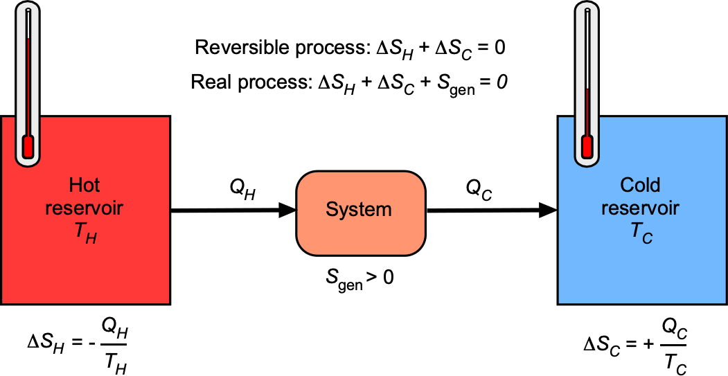
 .
.A reversible process is an idealization in which both the system and its surroundings can be returned to their initial states without any net changes elsewhere. In practice, aerospace propulsion systems operate under inherently irreversible conditions. Friction, turbulence, shock waves, chemical reaction irreversibility, and heat transfer across finite temperature differences all contribute to the generation of entropy.
Compressors and turbines, for example, lose efficiency because of boundary-layer flow separation and viscous effects, causing the actual enthalpy rise or drop to deviate from the ideal isentropic value. Nozzles operating under supersonic conditions generate shocks that raise entropy and diminish thrust. Combustors add further irreversibilities through incomplete combustion, mixing losses, and thermal gradients.
On a control volume basis, the entropy balance takes the general form
(69) 
where is the specific entropy,  is the boundary temperature at which the heat transfer occurs, and
  is the entropy generation rate caused by irreversibilities such as friction, mixing, and shock waves. This last term vanishes only for a perfectly reversible process, which remains an idealization. In real aerospace propulsion devices, entropy generation is unavoidable, setting an absolute limit on performance and efficiency.
Carnot Cycle & Efficiency Limits
The two main applications of thermodynamics are power generation and refrigeration. Devices that produce power are called engines, which operate on thermodynamic power cycles. Devices that provide a refrigeration effect, such as refrigerators, air conditioners, and heat pumps, operate on thermodynamic refrigeration cycles.
If the working fluid remains entirely in the gaseous phase throughout the cycle, the system is classified as a gas cycle. In contrast, if it undergoes a phase change and is partly liquid, such as steam, the system is classified as a vapor cycle. A cycle is considered closed if the working fluid is returned to its initial state at the end of the cycle and is then recirculated. In contrast, an open cycle involves renewing the working fluid at the end of each cycle.
The thermal efficiency of any power cycle is defined as the ratio of net work output to the heat input, i.e.,
(70) 
whether expressed in total or specific terms. The Carnot cycle establishes the maximum possible efficiency of any heat engine operating between two thermal reservoirs at temperatures  and
and  , i.e.,
(71) 
The Carnot cycle provides the theoretical upper limit for efficiency, but practical power cycles are modeled by more realistic processes. This fundamental result demonstrates that efficiency depends solely on the temperature ratio, regardless of the working substance or the cycle’s details. In aerospace propulsion, real engine cycles, such as the Brayton, Otto, Diesel, and rocket cycles, must continuously operate below this theoretical maximum.
The Carnot cycle is impractical for propulsion devices, but it provides the essential benchmark against which the performance of real engines can be judged.
Second Law Efficiencies
The performance of real aerospace devices is limited by irreversibilities such as friction, turbulence, and losses through shock waves. To quantify these effects, each device is compared to an idealized reversible process in which entropy is constant (isentropic process). The ratio of ideal to actual performance defines an isentropic efficiency. The concept of isentropic efficiency provides a convenient way to quantify the losses in practical components relative to their idealized, reversible counterparts.
For a compressor, a given pressure ratio requires a larger actual enthalpy rise than in the ideal isentropic case. This efficiency is defined as
(72) 
where is the enthalpy at the exit state if the compression were to be isentropic.
In a turbine, the actual enthalpy drop is smaller than the ideal isentropic enthalpy drop for the same pressure ratio. The efficiency is expressed as
(73) 
where is the enthalpy at the turbine exit in the ideal isentropic expansion.
For a nozzle, the actual exhaust velocity is less than the ideal isentropic value obtained for a given stagnation-to-ambient expansion. The nozzle efficiency is written as
(74) 
These efficiencies measure how closely real devices approach the reversible limit. A value of unity, although practically unattainable, corresponds to an ideal isentropic process, while lower values reflect greater entropy generation.
The Second Law sets the ultimate bounds on propulsion performance. Compressors and turbines require multiple stages to reduce losses, supersonic nozzles must be carefully contoured to minimize shock irreversibility, and even advanced rocket engines cannot convert all chemical energy into thrust. Minimizing entropy generation remains a guiding principle of aerospace thermodynamics.
Entropy, Availability, & Exergy Analysis
The Second Law of Thermodynamics not only establishes that entropy must increase in real processes, but also introduces the idea that not all energy can be converted into useful work. In aerospace propulsion, this is a crucial concept because the chemical energy of fuel or the enthalpy of a hot gas stream must be transformed into thrust or shaft power. However, irreversibilities limit the amount of that energy available for practical purposes. The framework for quantifying this applicable portion is called exergy analysis.
Entropy Generation & Irreversibility
When entropy is generated in a process, part of the available energy is degraded into a form that cannot be recovered as useful work. The entropy balance for a control volume is
(75) 
where represents entropy generation. This term quantifies irreversibilities resulting from friction, turbulence, mixing, chemical reactions, and shock waves. In aerospace systems, minimizing  is directly linked to maximizing an engine’s efficiency.
Availability (Exergy)
Availability or exergy is the maximum theoretical work that can be obtained from a system when it comes into equilibrium with its surroundings. It measures the useful portion of the energy relative to a reference environment. For aerospace propulsion, the “environment” is typically defined as the atmospheric values at ambient stagnation temperature and corresponding pressure  .
.
The specific flow exergy (per unit mass) is defined as
(76) 
where , , and are the local flow properties, and the subscript 0 denotes the reference environment. The first term,  , represents the enthalpy above the environmental levels and is often referred to as the thermal availability. The second term,
  , corresponds to the unavailable portion of the energy associated with entropy. The last two terms, and , account for the kinetic and potential energy contributions, respectively.
This formulation highlights the direct connection between thermodynamics and propulsion, as it quantifies the portion of the flow energy that can, in principle, be converted into thrust or shaft power under ideal conditions.
Exergy Destruction
In real processes, exergy is destroyed by irreversibility. The rate of exergy destruction is proportional to entropy generation, i.e.,
(77) 
which shows that every increment of entropy generation reduces the maximum useful work that could be extracted.
In a compressor, irreversibilities such as viscous losses and boundary layers degrade the exergy of the flow. In turbines, additional sources of destruction include leakage through tip clearances and shock interactions in transonic or supersonic stages. In a nozzle, shock waves and non-isentropic expansions generate entropy, diminishing the thrust that could otherwise be obtained. In a combustor, the dominant causes are chemical irreversibility and incomplete combustion, both of which reduce the available energy in the products. Taken together, these examples illustrate how an exergy analysis provides a unifying framework for quantifying losses across all propulsion components.
Exergy Efficiency
While the isentropic efficiencies can be used to compare real processes to reversible baselines, exergy efficiency measures how effectively available energy is utilized, i.e.,
(78) 
For example, in a gas turbine, the exergy input is the chemical exergy of the fuel, and the exergy output is the useful shaft power or jet thrust. In rocket engines, an exergy analysis reveals how much of the chemical potential of propellant is lost to irreversibility in mixing, combustion, and nozzle expansion.
Implications for Aerospace Propulsion
An exergy analysis highlights where improvements can yield the most significant gains in propulsion efficiency. In compressors and turbines, for example, pressure ratios are distributed across multiple stages, allowing each stage to operate much closer to an ideal reversible process, thereby reducing irreversibility. In nozzles operating at supersonic speeds, careful contouring is necessary to prevent shock waves and minimize entropy generation.
Within combustors, the designs aim for nearly complete and uniform burning, as incomplete combustion and poor mixing result in substantial exergy destruction. Ultimately, the success of high bypass ratio turbofans hinges on accelerating a large mass flow with only a small velocity change, thereby minimizing the kinetic energy and exergy carried away in the exhaust.
Ultimately, the Second Law and an exergy analysis provide not just a statement of thermodynamic limits, but also a diagnostic framework. By identifying where entropy is generated and exergy is destroyed, engineers can focus design efforts on minimizing irreversibility and maximizing the useful work obtained from each component of a propulsion system.
Isentropic Relations
It has been discussed why the Second Law establishes that real aerospace propulsion processes are inherently irreversible, with entropy generation caused by friction, turbulence, shock waves, and finite temperature gradients. Nevertheless, it is often helpful to consider the limiting case of a process that is both adiabatic and reversible. Such an idealization, known as an isentropic process, serves as a reference standard against which the performance of real compressors, turbines, diffusers, and nozzles can be evaluated.
By assuming no heat transfer and no entropy generation, the governing relations among pressure, temperature, and density take on elementary forms, allowing for the definition of ideal flow-property ratios that serve as benchmarks for evaluating efficiency. For an ideal gas undergoing such a process, the basic relations among pressure, temperature, and density ratios are
(79) 
where is temperature, is pressure, is density, and is the ratio of specific heats. These relations follow from combining the ideal-gas law with the condition of constant entropy.
In compressible flows, it is convenient to express the same results in terms of the Mach number  , where is velocity and is the local speed of sound. The total (stagnation) to static property ratios for an isentropic process are
(80) 
(81) 
(82) 
These equations are fundamental in aerospace applications because they help to define the ideal performance of compressors, turbines, diffusers, and nozzles. For example, the nozzle relations give the maximum achievable velocity for a given stagnation-to-ambient pressure ratio. Deviations from these relations in practice are captured by isentropic efficiencies, which quantify the irreversibilities in real devices.
The Third Law of Thermodynamics
The Third Law of Thermodynamics pertains to the behavior of entropy as the temperature approaches absolute zero. It states that the entropy of a perfect crystalline substance approaches zero as the absolute temperature tends to zero, i.e.,
(83) 
This principle, also known as the Nernst heat theorem, was first formulated by Walther Nernst in 1906. It implies that absolute zero cannot be reached in a finite number of steps, because as temperature decreases, further removal of energy becomes progressively more difficult. Whereas the First Law establishes the conservation of energy and the Second Law establishes the direction of processes and the inevitability of irreversibility, the Third Law provides an absolute reference for entropy.
In practical terms, the Third Law is less directly applied in aerospace analysis than the First and Second Laws. Its importance lies in defining a consistent zero point for entropy, without which entropy could only be measured in relative terms. By fixing the reference at = 0, the Third Law ensures that entropy values in thermodynamic property tables and equations of state are uniquely defined. This allows engineers to calculate enthalpies, entropies, and free energies with consistency, forming the basis for accurate analysis of gases used in propulsion systems. Cryogenic rocket propellants such as liquid hydrogen and liquid oxygen are analyzed using property data anchored to this entropy reference, making the Third Law applicable to spaceflight.
Summary of the Laws of Thermodynamics
Zeroth Law: If two systems are each in thermal equilibrium with a third, they are in thermal equilibrium with each other. This establishes temperature as a measurable and transitive property.
First Law: Energy is conserved. For any system, , and energy can be transformed but not created or destroyed.
Second Law: Entropy never decreases. For any process, i.e.,
![\[ dS \geq \frac{\delta Q}{T}, \qquad \oint \frac{\delta Q}{T} \leq 0 \]](https://eaglepubs.erau.edu/app/uploads/quicklatex/quicklatex.com-bc3703be4e09f6970c452ae0c57a7fb6_l3.svg "Rendered by QuickLaTeX.com")
with equality for reversible processes. Perfect conversion of heat into work is impossible.
Third Law: As  , the entropy of a perfect crystalline substance approaches zero, i.e.,
![\[ \lim_{T \to 0} S = 0 \]](https://eaglepubs.erau.edu/app/uploads/quicklatex/quicklatex.com-d4d45dd96d92c496396675a4125f7e63_l3.svg "Rendered by QuickLaTeX.com")
This law provides an absolute reference for entropy values.
Thermodynamics of Internal Combustion Engines
An internal combustion (IC) engine is a device in which the combustion of a fuel with an oxidizer, most often ambient air, occurs within the engine itself, as illustrated in the schematic below. The fundamental idea is that the chemical energy in the fuel is released through combustion, producing hot, high-pressure gases. These gases expand within the engine and either perform work directly on the moving parts, such as rotors, pistons, or turbine blades, or are accelerated out of the engine to generate a propulsive jet, similar to a rocket.
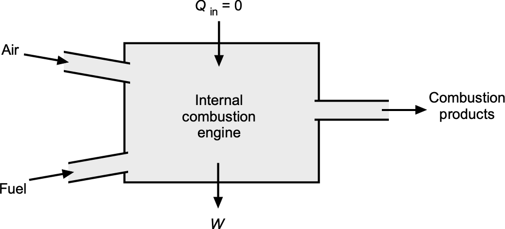
The overall energy transformation may be summarized as
(84) 
This description is entirely general and applies to all forms of IC engines. Reciprocating piston engines, rotary engines, gas turbines, and jet engines are all specific realizations of the same principle: the direct conversion of fuel chemical energy into useful mechanical power or thrust through combustion within the engine. In every case, the outputs also include exhaust products and waste heat, which are necessary byproducts because no engine can achieve 100% efficiency.
Gas Power Thermodynamic Cycles
The First and Second Laws of thermodynamics describe how energy and entropy change in individual processes. In practice, aerospace propulsion and power systems are built around complete thermodynamic cycles, where the working fluid undergoes a series of processes and then ultimately returns to its initial state. The net effect of a cycle is to produce useful work from a flow (as in engines and turbines) or to absorb work otherwise, such as to drive a pump or compressor.
Thermodynamic cycles are central to aerospace engineering analyses because they set the limits of propulsive performance. The thermal efficiency of a piston engine, the specific thrust of a turbojet, and the exhaust velocity of a rocket all trace back to the principles of these idealized cycles, corrected for actual irreversibilities. By studying the classic cycles, engineers can then identify what is achievable, what is lost to irreversibility, and where design improvements have the most significant impact. Although there are more, five cycles are important in aerospace applications:
- Otto cycle: The model for spark-ignition piston engines, relevant to all types of piston-powered airplanes.
- Diesel cycle: The model for compression-ignition engines, although not widely used in aviation.
- Brayton cycle: The fundamental cycle for gas turbines, turbofans, turbojets, and turboprops, making it the workhorse of modern aviation.
- Rankine cycle: A vapor power cycle, not typical for flight propulsion, but essential in auxiliary and space-based power systems.
- Rocket propulsion cycles: Variants of open and closed cycles that rapidly convert chemical energy directly into high-velocity exhaust jets to produce thrust.
Otto Cycle (Spark-Ignition Engines)
The Otto cycle is the idealized thermodynamic cycle that represents the operation of a spark-ignition piston-powered IC engine. Named after Nikolaus Otto, who built the first successful four-stroke piston engine in 1876, the cycle represents the basis of modern gasoline-fueled engines. It consists of four internally reversible processes for a fixed mass of working gas in the form of an air-fuel mixture, typically modeled just as air alone as an ideal gas.
Process Stages
The cycle begins at state 1, with the piston at bottom dead center (BDC), and the cylinder is filled with the fuel-air mixture, as shown in the figure below, which is obtained by opening the inlet valve. The first process, state 1 to 2, is an isentropic compression in which the piston moves upward in the cyclinder with the inlet and exhaust valves closed, reducing the cylinder volume from the maximum value  at bottom dead center (BDC) to the minimum value
  at top dead center (TDC). The pressure and temperature rise significantly during this compression process, but no heat is exchanged with the surroundings. The ratio
  is called the compression ratio of the engine, and is typically at least 8.5:1 in normally aspirated (non-supercharged) forms. Supercharging can significantly increase the compression ratio, which is intended to enhance the engine’s power output.
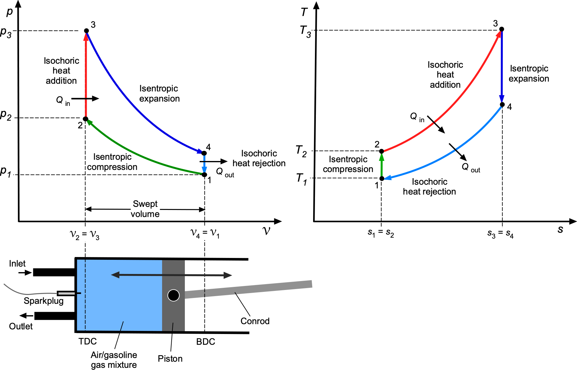 and diagrams of the Otto cycle.
The second process, from state 2 to state 3, represents the rapid combustion of the mixture, which is ignited by the spark plug. In the ideal cycle, this is modeled as a constant-volume heat addition, so the volume remains fixed at while the pressure and temperature rise abruptly as an amount of heat  is supplied to the gas. The third process, from state 3 to 4, is an isentropic expansion. The piston moves downward from TDC back to BDC, increasing the volume from to . During this expansion, the hot gas does work on the piston, causing the pressure and temperature to fall accordingly. This is the power stroke of the engine. The fourth process, state 4 to 1, closes the cycle. This is a constant-volume heat rejection process in which the exhaust valve opens, allowing the remaining waste thermal energy to be discharged into a pipe and subsequently into the surrounding atmosphere. The pressure and temperature drop suddenly at fixed volume by an amount corresponding to the rejected heat,
  .
.
Process Diagrams
The ideal diagram of the Otto cycle (shown in the figure above) consists of two adiabatic (isentropic) curves, representing compression and expansion, joined by two vertical constant-volume lines, representing the parts of the cycle where heat is added and heat is rejected. On the diagram, the compression and expansion legs are curves because isentropic processes follow  constant. Because the force on the piston is the instantaneous cylinder pressure times the piston area, i.e.,
  , the incremental work during an infinitesimal piston displacement
  is
is
(85) 
The corresponding change in cylinder volume is  , then over one complete thermodynamic cycle, the net work is
(86) 
which is the (signed) area enclosed by the closed loop on the – diagram. A counterclockwise loop gives (engine: net work output), whereas a clockwise loop gives  (compressor/pump: net work input).
The corresponding diagram shows two vertical isentropic lines and two curves of constant-volume segments. During the constant volume process from state 2 to 3, heat is added to the gas, raising its temperature from to  . Conversely, during the process from state 4 to 1, heat is rejected, reducing the temperature from
  back to . The heat-addition and rejection legs are logarithmic curves given by . On a diagram, the integral
(87) 
represents the heat transfer, where the area enclosed by a closed loop indicates the net heat exchanged, which equals the net work of the cycle according to the First Law of Thermodynamics. The heat interactions are, therefore,
(88) 
so the net work is  . From the isentropic compression and expansion relations, then
(89) 
where  is the compression ratio. Substituting these relations gives the thermal efficiency of the Otto cycle as
(90) 
which shows that efficiency depends only on compression ratio and specific heat ratio. In practice,  is limited by the onset of pre-ignition or “knock,” which is tied to the octane rating of the fuel.
Diesel Cycle (Compression-Ignition Engines)
The Diesel cycle is the idealized thermodynamic model for compression-ignition internal combustion engines. First demonstrated by Rudolf Diesel in 1897, it utilizes self-ignition or auto-ignition, in which fuel is injected into highly compressed, hot air, causing it to burn spontaneously. Diesel engines are valued for their high efficiency, durability, and the ability to operate on heavier fuels compared to gasoline engines. They are used extensively for automobiles, trucks, buses, ships, locomotives, and stationary power generation. In aerospace, their application has been more limited, although lightweight compression-ignition engines have been adapted for certain UAVs and light aircraft.
The efficiency advantage of diesel engines primarily stems from their high compression ratios, which enable more complete combustion and higher thermal efficiency compared to spark-ignition engines. Their robust construction also provides them with a long service life and the ability to withstand continuous high-load operation. However, disadvantages include greater weight, higher initial cost, and increased emissions of particulates and nitrogen oxides, which require sophisticated after-treatment systems to meet environmental standards.
Process Stages
The Diesel cycle consists of four internally reversible processes applied to a fixed mass of an ideal gas, as shown in the figure below. The first process, from state 1 to state 2, is an isentropic compression from the maximum cylinder volume at BTC to the clearance volume at TDC, which raises pressure and temperature without heat transfer. The second process, from state 2 to 3, involves adding heat under constant pressure. During this stage, fuel is injected through the inlet valve and burns spontaneously because of the high air temperature. Simultaneously, the piston moves downward in the cylinder, increasing temperature and volume from to  at essentially a fixed pressure. The third process, from state 3 to 4, is an isentropic expansion back to , during which the gas does work on the piston, and its pressure and temperature decrease. The fourth process, from state 4 to 1, is a constant-volume heat rejection that occurs after the exhaust valve opens, reducing pressure and temperature at a fixed volume to complete the cycle.
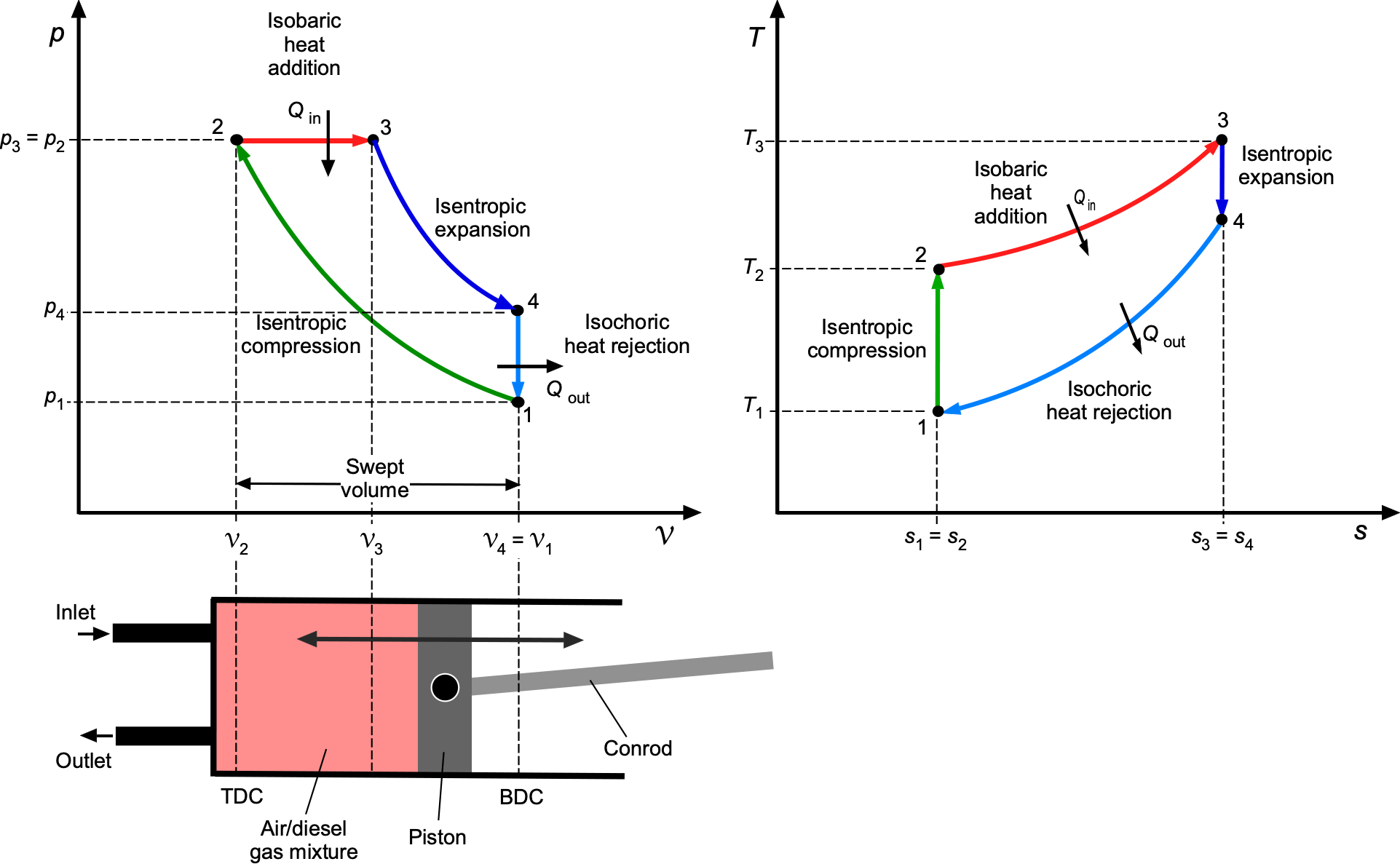 and diagrams of the Diesel cycle.
Process Diagrams
The ideal diagram of the Diesel cycle consists of two adiabatic (isentropic) curves, representing compression and expansion, joined by a horizontal constant-pressure line for heat addition and a vertical constant-volume line for heat rejection. The heat-addition and rejection legs are logarithmic curves given by . The corresponding diagram has two vertical isentropic lines, a curve representing constant-pressure heat addition, and another curve representing constant-volume heat rejection. Heat input occurs during states 2 to 3 at a constant pressure, while heat is rejected during states 4 to 1 at a constant volume.
The heat interactions are
(91) 
with the net work . Using the temperature relations for isentropic compression and expansion, then
(92) 
and noting that  , where is the compression ratio and
  is the cutoff ratio. Therefore, the efficiency becomes
(93) 
This expression indicates that Diesel efficiency depends on both the attainable compression ratio and the cutoff ratio. Higher compression ratios yield improved performance, and the cutoff ratio moderates the effect of heat addition. In practice, Diesel engines often achieve higher indicated and brake thermal efficiencies than comparable spark-ignition engines, particularly at reduced loads, because they tolerate higher compression ratios and operate with overall lean mixtures.
Cycle Work and Power
For any reciprocating engine, the cylinder volume varies between the clearance volume at TDC, denoted  , and the maximum volume at BDC, denoted
  . The displacement (swept) volume is.
  . It is convenient to normalize this to the displacement volume by defining the indicated mean effective pressure (IMEP), i.e.,
(94) 
This value is the hypothetical equivalent constant pressure which, if applied during the expansion over  , would yield the same net cycle work. If the crankshaft rotates at
  revolutions per minute and the engine has
  cylinders, the cycle frequency per cylinder is
  for a four-stroke cycle and
  for a two-stroke cycle, expressed in cycles per second. The indicated power of the engine is then
(95) 
Therefore, the power produced from the Otto or Diesel cycles is directly proportional to the loop area on the diagram, the total displacement volume, and the number of rotational cycles per second.
Supercharging and Turbocharging
Aircraft piston engines operating on the Otto or Diesel cycles experience a progressive loss of power with increasing altitude. The underlying reason is the decrease in ambient air pressure and density at higher altitudes, which reduces the mass of air inducted into the engine per cycle. Because engine power depends directly on the mass of the air-fuel mixture that can be compressed and burned, altitude severely limits the performance of a normally aspirated intake system. The solution is to raise the intake pressure by compressing the air before it enters the cylinder, a process known as forced induction, which increases the IMEP value.
Supercharging refers to the use of a mechanically driven compressor, powered directly by the crankshaft, to increase the manifold pressure. Turbocharging utilizes a turbine positioned in the exhaust stream to harness energy from the exhaust gases, which then drives a compressor. Both methods achieve the same basic goal of raising the pressure and density of the intake charge, restoring power that would otherwise be lost at altitude. In either case, the thermodynamic process involves compressing the working fluid before the cycle begins.
For an ideal gas undergoing an isentropic compression process, the relation between pressure and temperature is
(96) 
but in all compressors, the actual temperature rise exceeds this ideal value. An intercooler can be used between compression stages to lower the air temperature, reducing the work required for compression and increasing the overall efficiency. The isentropic efficiency can be introduced to quantify the irreversibilities, i.e.,
(97) 
where  is the ideal (isentropic) exit temperature for a given pressure ratio and is the actual exit temperature. This framework applies equally to mechanically driven superchargers and turbine-driven turbochargers.
The effect of turbo-boosting can be visualized directly on the and diagrams of the Otto and Diesel cycles. In the diagram, compression begins from a higher intake pressure, so the entire cycle is elevated relative to the unboosted case. This increases both the indicated mean effective pressure and the net work per cycle. On the diagram, shifting the intake state to higher pressure and temperature changes the initial entropy reference line and modifies the subsequent compression and expansion paths. The practical benefit is that the enclosed cycle area, proportional to the work output, increases with turboboosting, even though the fundamental thermodynamic cycle remains the same.
In spark-ignition (Otto) engines, the degree of supercharging is limited by the onset of pre-ignition or knock, which constrains the maximum compression ratio. In compression-ignition (Diesel) engines, supercharging is widely used to improve both power and efficiency because knock is not a limiting factor. In modern practice, turbochargers driven by the exhaust gases are the most common method used to boost the power from a Diesel engine.
Check Your Understanding #3 – Power from a single cylinder piston engine
A single-cylinder four-stroke engine has a displacement volume = 500 cm = 5.0
= 5.0 m and operates at = 3,000 rpm. The indicated mean effective pressure is
  = 900 kPa. Determine the net indicated work per cycle and the indicated power output for this engine.
Show solution/hide solution.
The net indicated work per cycle is found by multiplying the IMEP by the displacement volume. With  and
and  , the result is
![\[ W = \mathrm{IMEP}\,\mathcal{V}_d = (9.0\times 10^{5})(5.0\times 10^{-4}) = 450~\mathrm{J/cycle}. \]](https://eaglepubs.erau.edu/app/uploads/quicklatex/quicklatex.com-f68383417b78cf2fec37538adb7cd8aa_l3.svg "Rendered by QuickLaTeX.com")
In a four-stroke engine, one thermodynamic cycle is completed every two crankshaft revolutions. At 3,000 rpm, the cycle frequency is
![\[ f_{\rm cyc} = \frac{N}{120} = \frac{3000}{120} = 25~\mathrm{cycles/s}. \]](https://eaglepubs.erau.edu/app/uploads/quicklatex/quicklatex.com-30c16f53dcc6e7a12b379145ae0b9b8b_l3.svg "Rendered by QuickLaTeX.com")
Multiplying the work per cycle by the cycle frequency gives the indicated power for this single cylinder, i.e.,
![\[ P_{\rm ind} = f_{\rm cyc}\,W = 25 \times 450 = 1.125\times 10^{4}~\mathrm{W} = 11.25~\mathrm{kW} \]](https://eaglepubs.erau.edu/app/uploads/quicklatex/quicklatex.com-e4abaec3d8d21e54c3ddb149bce2d2c1_l3.svg "Rendered by QuickLaTeX.com")
Therefore, the engine develops about 11.3 kW of indicated power at these conditions. Notice that for a multi-cylinder engine, the total indicated power is obtained by multiplying by the number of cylinders.
Brayton Cycle (Gas Turbine Engines)
The Brayton cycle is the fundamental thermodynamic model for gas turbine engines, which power most of modern aviation in the form of turbojets, turbofans, and turboprops. First proposed in the 1870s by George Brayton for an early gas engine, the cycle became practical only with the development of axial compressors and turbines in the 20th century. It remains central to aerospace propulsion because it shows how chemical energy in fuel is transformed into a high-velocity exhaust jet, as in a turbojet, or into mechanical shaft work, as in turbofans and turboprops, to produce thrust.
Process Stages
The Brayton cycle comprises four internal processes, as illustrated in the schematic below. The first process is an isentropic compression, in which air is compressed adiabatically in the compressor from state 1 to state 2. The second process is constant-pressure heat addition, where the combustion of fuel in the combustor increases the temperature of the working fluid from state 2 to state 3, while maintaining essentially constant pressure. The third process is an isentropic expansion, during which the high-temperature gas expands adiabatically through the turbine, thereby producing shaft work that occurs from state 3 to state 4. The final process is constant-pressure heat rejection, which occurs through an exit nozzle.
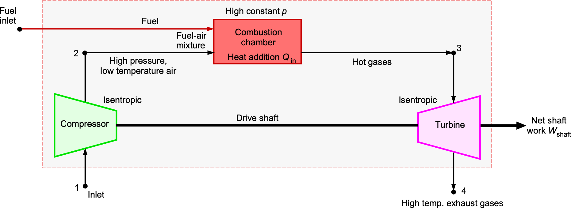
The Bayton cycle is, in principle, an open system. However, in the ideal Brayton cycle, the working fluid can be imagined to follow a closed loop, allowing for the consistent representation of thermodynamic processes with known elements of thermodynamic modeling, as shown in the figure below. Heat rejection from state 4 back to state 1 conceptually closes the cycle, even though in a real gas turbine, the exhaust is discharged to the atmosphere and replaced by new fresh air at the inlet. When the cycle is depicted in this manner, two external heat exchangers are necessary: one to add heat (the combustor) and another to reject heat, thereby returning the fluid to its initial state.
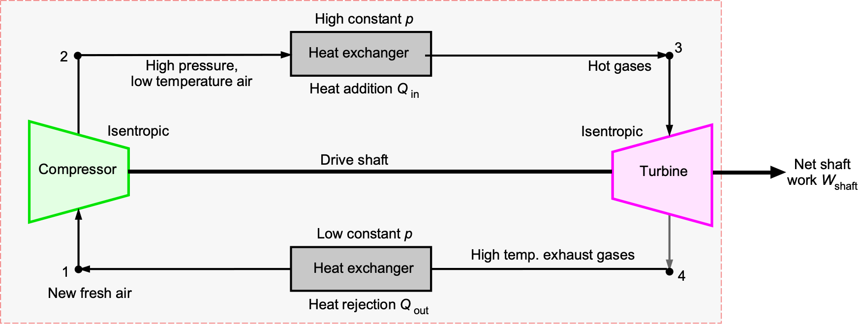
Process Diagrams
On the pressure-volume (–) diagram as shown in the figure below, the idealized Brayton cycle is represented by two adiabatic compression and expansion curves connected by two constant-pressure processes. The compression process from state 1 to 2 is an isentropic rise in pressure with decreasing volume, the heat addition process from state 2 to 3 is a horizontal line of constant pressure with increasing volume, the expansion process from 3 to 4 is an isentropic pressure drop with increasing volume, and the heat rejection process from 4 to 1 is a horizontal line at constant pressure returning to the initial state.
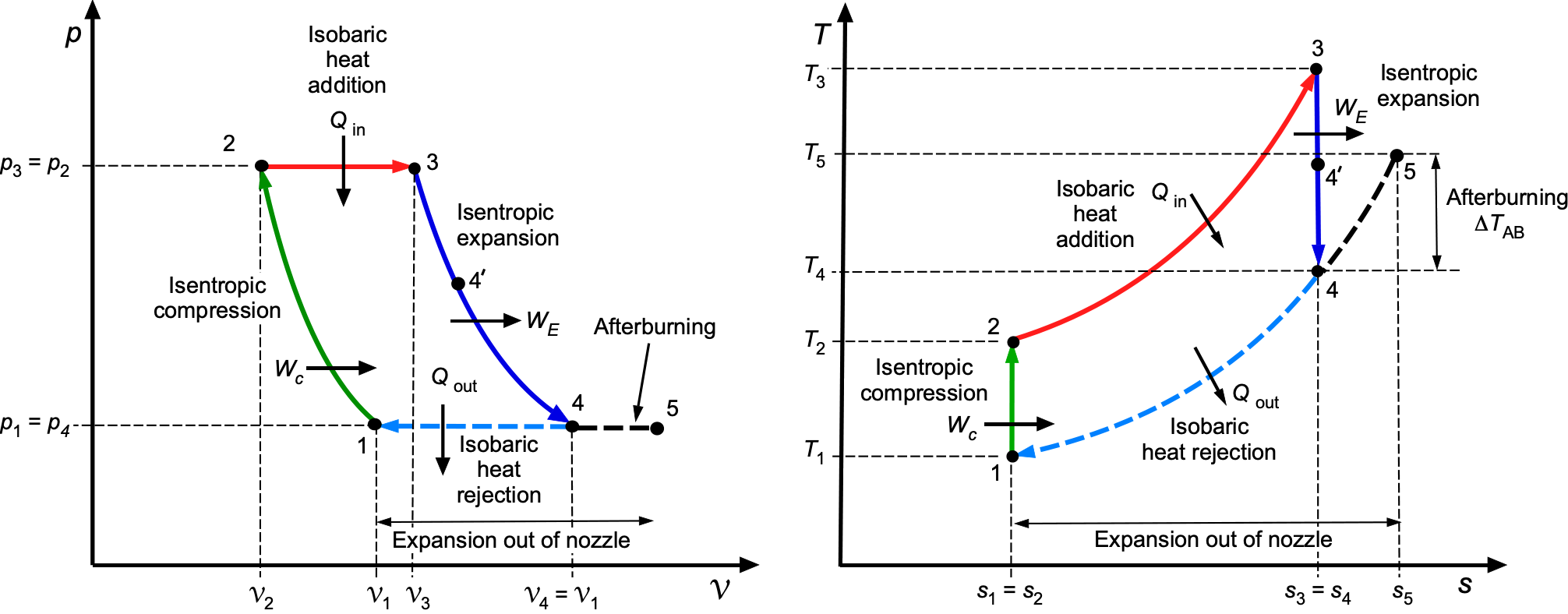 and process diagrams of the idealized Brayton cycle.
The corresponding diagram shows two vertical isentropic lines and two curved constant-pressure segments, forming a rectangle whose height corresponds to the temperature rise and whose width reflects the change in entropy. Heat is added during states 2 to 3 at constant pressure, while heat is rejected during states 4 to 1, also at constant pressure.
Notice that in most textbooks, the Brayton cycle is usually drawn as a closed loop on and diagrams, with a heat-rejection leg (shown here as a dashed line) returning to the initial state. In reality, a jet engine is an open cycle in that the working fluid enters once and is exhausted to the atmosphere. The state 4 to 1 process in the ideal Brayton cycle (or state 5 to ambient in the afterburning case) is only a conceptual closure, representing cooling in the environment under the principle of energy conservation. This simplification allows the use of cyclic analysis, while the actual engine operates continuously with the atmosphere providing the sink.
The heat interactions are
(98) 
and the turbine and compressor work values are
(99) 
so that  . From the isentropic relations, then
(100) 
where  is the compressor pressure ratio. Substituting gives the thermal efficiency as
(101) 
Therefore, the Brayton efficiency improves with increasing pressure ratio and turbine inlet temperature, subject to the practical limits of compressor design, materials, cooling, and weight (for an aircraft).
Back-Work Ratio
In a gas turbine cycle, the turbine must supply enough work to drive the compressor and provide useful net work for propulsion through a jet from a suitably shaped nozzle or as shaft power. The turbine’s work output is
(102) 
and the compressor work input is
(103) 
so that the net cycle work is
(104) 
The fraction of the turbine work that is consumed by the compressor is referred to as the back-work ratio (BWR). It is defined as
(105) 
A high value of the BWR means that a significant fraction of the turbine output is internally used to run the compressor, leaving less net work available. On the diagram shown above, this can be illustrated by splitting the turbine expansion into two steps, i.e., state 3 to 4′ supplies exactly the compressor work. In contrast, state 4′ to 4 represents the net turbine work output. In modern gas turbines, the back-work ratio is typically in the range of 40–60%. This analysis illustrates why gas turbine performance is highly dependent on achieving exceptionally high turbine inlet temperatures; the hotter the working fluid entering the turbine, the more expansion work is available to cover the compressor demand and still provide useful net power.
The significance of the BWR also depends on the type of gas turbine engine. In a turbojet or turbofan, the turbine is designed to extract just enough work to drive the compressor (and the fan in the case of a turbofan), with most of the remaining enthalpy reserved for expansion through the nozzle, producing thrust. Because of this balance, the BWR is high, often ranging from 0.45 to 0.55, meaning that nearly half of the turbine output is internally recycled, and only the remainder contributes to jet propulsion.
By contrast, in a turboshaft or turboprop engine, the turbine must deliver substantial shaft power to drive a rotor, propeller, or gearbox in addition to covering the compressor demand. This requires a much larger turbine expansion, so the compressor work is a smaller fraction of the total. The BWR in these engines is much lower, typically in the range of 0.2–0.3, with the majority of turbine output available as useful shaft power.
This comparison highlights that while the BWR is always a critical consideration in gas turbine analysis, its value and implications vary with the intended role of the engine. High BWRs in turbojets and turbofans emphasize the importance of achieving high turbine inlet temperatures and efficient compressors. In contrast, low BWRs in turboshafts and turboprops reflect the need to maximize shaft power output for propulsion.
Afterburning (Reheat) Cycle
The thrust of a turbojet (and some turbofans) can be increased temporarily by injecting fuel into the exhaust stream downstream of the turbine. This arrangement is called an afterburner or reheat system. The significant advantage of afterburning is the substantial increase in thrust, which is critical for takeoff and supersonic flight. A significant disadvantage is the very low thermal efficiency, as the afterburner consumes a large amount of fuel for a given amount of thrust. For this reason, afterburners are used only intermittently.
In thermodynamic terms, an afterburner can be represented as a Brayton cycle with an additional isobaric heat addition process between the turbine exit and the nozzle. The turbine still provides the work to drive the compressor, but the afterburner raises the total temperature of the exhaust stream before its expansion in the tailpipe. If is the turbine exit temperature, then afterburning increases the stagnation temperature to  , i.e.,
(106) 
where the  boost depends on the amount of fuel injected and burned.
The effect on the diagram shown above is an additional horizontal step (constant pressure heat addition) between the turbine exit and the nozzle inlet. On the corresponding diagram, the cycle does not change shape significantly; however, the expansion through the nozzle begins from a higher total temperature, resulting in a higher jet velocity and, consequently, greater thrust.
Connection to Carnot Efficiency
While the Otto, Diesel, and Brayton cycles describe the operation of real IC engines, it is useful to recall the Carnot efficiency. Carnot established that no heat engine operating between a hot reservoir at temperature and a cold reservoir at can exceed the limit
(107)
This limit follows from the reversible Carnot cycle, which consists of two isothermal and two adiabatic processes. On the process diagram, the process from state 1 to 2 is an isothermal expansion at with  and heat input
  , where is the specific gas constant per unit mass. The process from state 2 to 3 is a reversible adiabatic expansion to with
  constant.
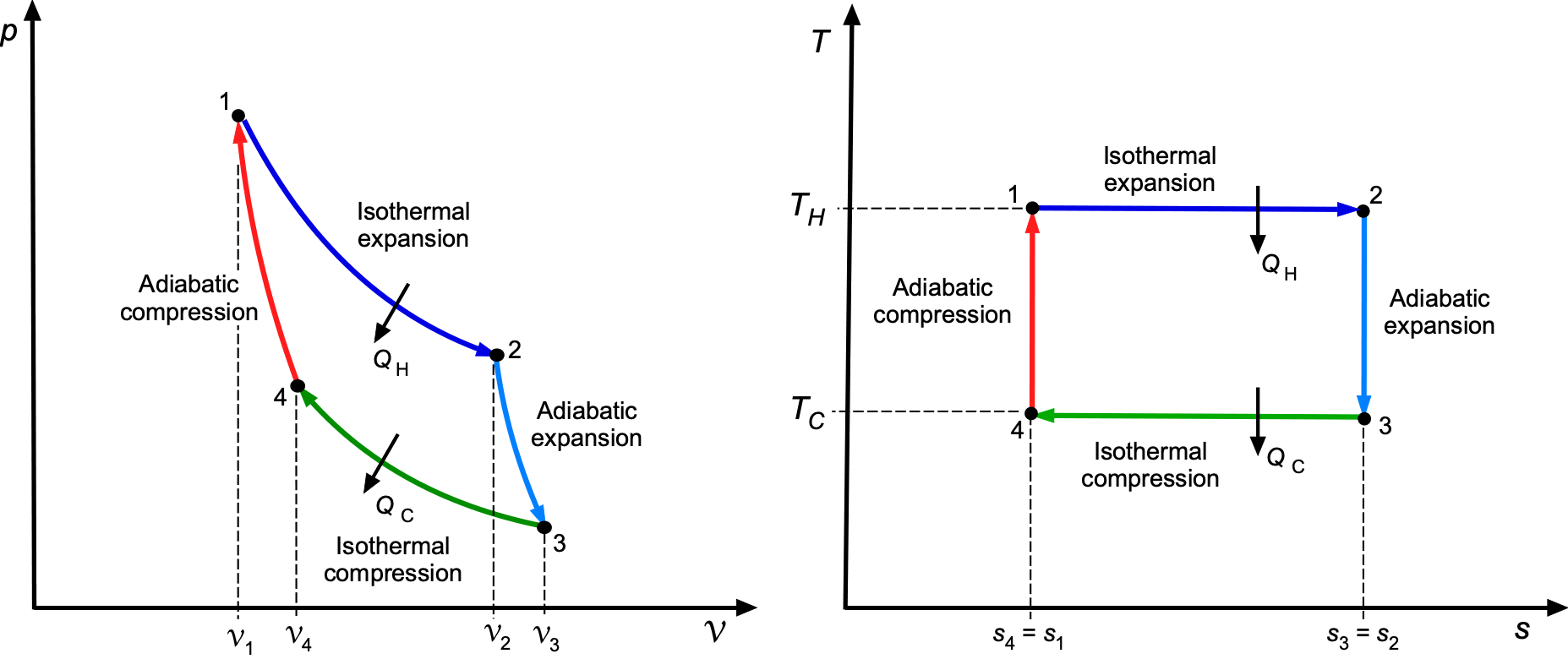 and diagrams of the Carnot cycle.
The process from state 3 to 4 is an isothermal compression at with  and heat rejection
  . Finally, the process from state 4 to 1 is a reversible adiabatic compression back to . The area enclosed equals the specific net work.
On the process diagram, the process from state 1 to 2 is a horizontal line at , process 2 to 3 is a vertical adiabat, process 3 to 4 is a horizontal line at , and process 4-1 is a vertical adiabat; the rectangular area equals the specific net work. Using  , the isothermal heats can be written as
(108) 
and
(109) 
The reversible adiabatic condition is
(110) 
Applying this result from states 2 to 3 and states 4 to 1 gives
(111) 
which implies
(112) 
The same logarithmic factor appears on both isotherms, so
(113) 
so that
(114) 
This argument is independent of the equation of state and shows that the Carnot result depends only on the reservoir temperatures and the assumption of reversibility.
For comparison, the idealized cycle efficiencies are
(115) ![\begin{eqnarray*} \eta_{\text{Otto}} & = & 1 - \frac{1}{r^{\gamma-1}} = 1 - \frac{c_v\,(T_4 - T_1)}{c_v\,(T_3 - T_2)} = 1 - \frac{T_4 - T_1}{T_3 - T_2} \\[6pt] \eta_{\text{Diesel}} & = & 1 - \frac{1}{r^{\gamma-1}} \left( \frac{\beta^{\gamma} - 1}{\gamma (\beta - 1)} \right) = 1 - \frac{c_v\,(T_4 - T_1)}{c_p\,(T_3 - T_2)} = 1 - \frac{1}{\gamma}\,\frac{T_4 - T_1}{T_3 - T_2} \\[6pt] \eta_{\text{Brayton}} & = & 1 - \frac{1}{r_p^{(\gamma-1)/\gamma}} = 1 - \frac{c_p\,(T_4 - T_1)}{c_p\,(T_3 - T_2)} = 1 - \frac{T_4 - T_1}{T_3 - T_2} \end{eqnarray*}](https://eaglepubs.erau.edu/app/uploads/quicklatex/quicklatex.com-78a29de23790ecdf8fb06576c75269af_l3.svg "Rendered by QuickLaTeX.com")
where is the compression ratio,  is the cut-off ratio for the Diesel cycle,
  is the compressor pressure ratio, and is the ratio of specific heats.
The temperature forms of the efficiencies show that the Otto and Brayton add and reject heat at the same constant condition, so the or terms cancel out. In contrast, the Diesel cycle combines constant-pressure and constant-volume processes, introducing the  factor. The Carnot limit for high-temperature combustion, with
  2,000 to 2,500 K and ambient
  300 K, is on the order of 85 to 88%. Real engines fall well below this ceiling, with even the best modern designs being about half of the theoretical maximum, as shown in the figure below.
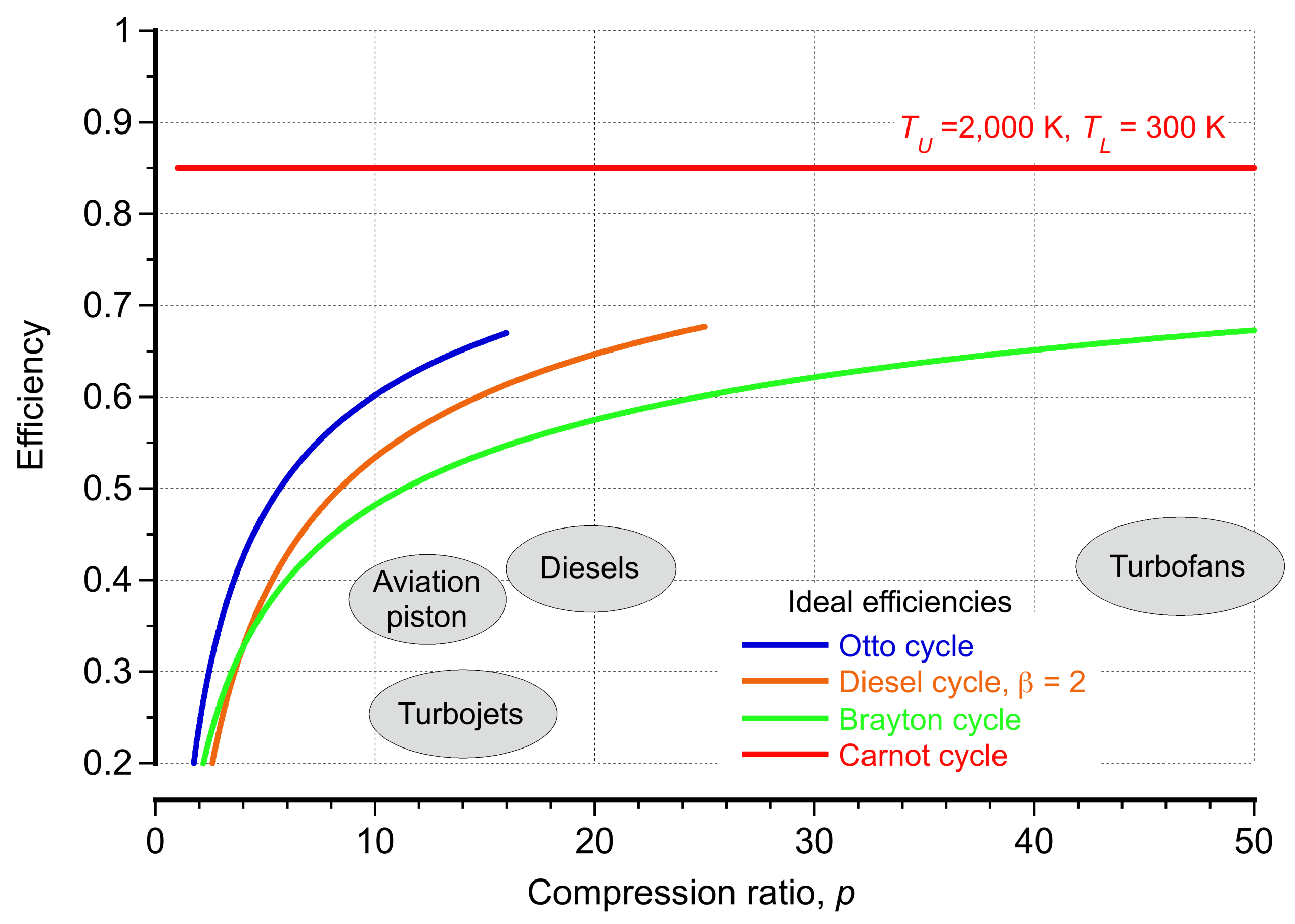
For the Otto cycle (spark-ignition engines), the ideal air-standard efficiency ranges from 55 to 65% for compression ratios between = 8 and 12. In practice, modern gasoline engines achieve a thermal efficiency of 30 to 36%, with optimized variants reaching up to 40%. These values are limited by pre-ignition (knock), heat transfer, and the finite time available for combustion within each cycle.
In the Diesel cycle (compression-ignition engines), ideal efficiencies can reach 60 to 70% for compression ratios of = 14 to 20 with modest cut-off ratios. Practical heavy-duty diesels can achieve 40 to 46%, and advanced designs have been reported to approach 50%. Higher cut-off ratios reduce the ideal efficiency, and in real engines, additional losses arise from incomplete combustion and heat transfer.
The Brayton cycle (used in gas turbines) has an ideal efficiency of approximately 55 to 60% for pressure ratios of = 30 to 40 and  1.33. In practice, large industrial gas turbines have been reported to achieve efficiencies of up to 60%. Gas turbines for airplanes, however, are limited to efficiencies of approximately 35 to 40% at cruise conditions because of turbine inlet temperature restrictions, cooling requirements, compressor inefficiencies, and weight limitations.
Therefore, while real cycles approach only about half of the Carnot limit at best, the ordering of efficiencies remains consistent, i.e.,
(116) 
with all three remaining strictly below  .
.
As previously discussed, supercharging or turbocharging raises the intake pressure and density before compression. In the Otto cycle, the ideal efficiency expression depends only on , so supercharging does not directly alter the cycle efficiency. However, the higher intake pressure increases the mass of fuel/air charge per intake cycle, thereby increasing the engine’s power output. In practice, pre-ignition(knock) limits constrain the maximum usable , so any efficiency benefit is relatively small.
In the Diesel cycle, however, supercharging can also improve efficiency, because the same power can be obtained with a smaller cut-off ratio , which corresponds to a higher cycle efficiency. In both cases, supercharging increases the peak cycle temperature , moving the cycle closer to the Carnot limit. In the Brayton cycle, afterburning reduces efficiency because the exhaust gases do not drive the compressor turbine, thus sacrificing efficiency for short bursts of additional thrust.
Check Your Understanding #4 – Brayton cycle efficiency
Air enters a turbojet engine at = 300 K. The compressor pressure ratio is = 12 , and the turbine inlet temperature is = 1,400 K. Assume constant properties = 1,004 J kg K, and = 1.4. For the real Brayton cycle, the compressor and turbine have isentropic efficiencies of  = 0.85 and
  = 0.88. Calculate the thermal efficiency and back-work ratio for both the ideal and real cycles.
Show solution/hide solution.
For the ideal Brayton cycle, the isentropic temperature rise through the compressor is
![\[ T_{2s} = T_1 \, r_p^{(\gamma-1)/\gamma} \]](https://eaglepubs.erau.edu/app/uploads/quicklatex/quicklatex.com-1f17569d3cc3c2b783d390eb9d5729c0_l3.svg "Rendered by QuickLaTeX.com")
which gives  . The isentropic temperature drop through the turbine is
![\[ T_{4s} = T_3 \, r_p^{-(\gamma-1)/\gamma} \]](https://eaglepubs.erau.edu/app/uploads/quicklatex/quicklatex.com-dc56d7bcacb614cee1752034f626e3c5_l3.svg "Rendered by QuickLaTeX.com")
which gives  . The compressor work is
![\[ W_c = c_p (T_{2s} - T_1) = 311~\mathrm{kJ/kg} \]](https://eaglepubs.erau.edu/app/uploads/quicklatex/quicklatex.com-a2c265545abceed06ea11d478cb3e850_l3.svg "Rendered by QuickLaTeX.com")
The turbine work is
![\[ W_t = c_p (T_3 - T_{4s}) = 715~\mathrm{kJ/kg} \]](https://eaglepubs.erau.edu/app/uploads/quicklatex/quicklatex.com-0dcb001655c2a9973680785ff5b3a179_l3.svg "Rendered by QuickLaTeX.com")
and the heat input is
![\[ Q_{\text{in}} = c_p (T_3 - T_{2s}) = 793~\mathrm{kJ/kg} \]](https://eaglepubs.erau.edu/app/uploads/quicklatex/quicklatex.com-85c81383aa9da1b1014bd55cbe1b8b42_l3.svg "Rendered by QuickLaTeX.com")
The net work output is
![\[ W_{\text{net}} = W_t - W_c = 403~\mathrm{kJ/kg} \]](https://eaglepubs.erau.edu/app/uploads/quicklatex/quicklatex.com-ada9b53b771284e30553e4963cad20ee_l3.svg "Rendered by QuickLaTeX.com")
so the thermal efficiency is
![\[ \eta_{\text{ideal}} = \frac{W_{\text{net}}}{Q_{\text{in}}} = 0.51 \]](https://eaglepubs.erau.edu/app/uploads/quicklatex/quicklatex.com-7b12b297ae8703a46014869f060ee03b_l3.svg "Rendered by QuickLaTeX.com")
The back-work ratio is
![\[ \mathrm{BWR} = \frac{W_c}{W_t} = 0.44 \]](https://eaglepubs.erau.edu/app/uploads/quicklatex/quicklatex.com-1fc6c55870e21756abf906522aba65c1_l3.svg "Rendered by QuickLaTeX.com")
For the real Brayton cycle, the actual compressor outlet temperature is obtained from
![\[ \eta_c = \frac{T_{2s} - T_1}{T_2 - T_1} \]](https://eaglepubs.erau.edu/app/uploads/quicklatex/quicklatex.com-91ae0965fa2fb85ccb9ca141777bd4ed_l3.svg "Rendered by QuickLaTeX.com")
so that
![\[ T_2 = T_1 + \frac{T_{2s} - T_1}{\eta_c} = 665~\mathrm{K} \]](https://eaglepubs.erau.edu/app/uploads/quicklatex/quicklatex.com-16ba6abd09e8e561c306bbef1d4e7a4a_l3.svg "Rendered by QuickLaTeX.com")
The compressor work is then
![\[ W_c = c_p (T_2 - T_1) = 366~\mathrm{kJ/kg} \]](https://eaglepubs.erau.edu/app/uploads/quicklatex/quicklatex.com-3b94bb77c0313166e9f8ee9033c5abbd_l3.svg "Rendered by QuickLaTeX.com")
For the turbine, the isentropic efficiency gives
![\[ \eta_t = \frac{T_3 - T_4}{T_3 - T_{4s}} \]](https://eaglepubs.erau.edu/app/uploads/quicklatex/quicklatex.com-355b10fc13c0860477bc36f69129d42d_l3.svg "Rendered by QuickLaTeX.com")
so that
![\[ T_4 = T_3 - \eta_t (T_3 - T_{4s}) = 774~\mathrm{K} \]](https://eaglepubs.erau.edu/app/uploads/quicklatex/quicklatex.com-e65054ef442ada52df718410edfd2dcd_l3.svg "Rendered by QuickLaTeX.com")
The turbine work is
![\[ W_t = c_p (T_3 - T_4) = 629~\mathrm{kJ/kg} \]](https://eaglepubs.erau.edu/app/uploads/quicklatex/quicklatex.com-09f7602154b2bfcbf627b1f4c24b9e7c_l3.svg "Rendered by QuickLaTeX.com")
and the heat input is
![\[ Q_{\text{in}} = c_p (T_3 - T_2) = 738~\mathrm{kJ/kg} \]](https://eaglepubs.erau.edu/app/uploads/quicklatex/quicklatex.com-b68f8e5581c70ebebe2ea5bfaad52017_l3.svg "Rendered by QuickLaTeX.com")
The net work is
![\[ W_{\text{net}} = W_t - W_c = 262~\mathrm{kJ/kg} \]](https://eaglepubs.erau.edu/app/uploads/quicklatex/quicklatex.com-33683b93b302e4d42db6b9eba6bb191b_l3.svg "Rendered by QuickLaTeX.com")
and so the thermal efficiency is
![\[ \eta_{\text{real}} = \frac{W_{\text{net}}}{Q_{\text{in}}} = 0.36 \]](https://eaglepubs.erau.edu/app/uploads/quicklatex/quicklatex.com-1d67482dc180934d79675b6622eff442_l3.svg "Rendered by QuickLaTeX.com")
The back-work ratio is
![\[ \mathrm{BWR} = \frac{W_c}{W_t} = 0.58 \]](https://eaglepubs.erau.edu/app/uploads/quicklatex/quicklatex.com-daa6be74da62c01b9dcaa98e8188d159_l3.svg "Rendered by QuickLaTeX.com")
This example shows that the ideal Brayton cycle efficiency is about 51%, but real component inefficiencies reduce it to 36%. The increase in back-work ratio from 0.44 to 0.58 illustrates how compressor and turbine irreversibilities consume a significant fraction of turbine output and reduce net work.
Rocket Propulsion Cycles
Rocket engines need both a fuel and an oxidizer (i.e., a propellant) carried onboard the vehicle. When they are suitably combined and burned, they produce high-temperature combustion products that are expanded through a nozzle to generate thrust, as shown in the schematic below. Thermodynamically, rockets can be regarded as specialized “open” Brayton systems, with propellant-fed turbopumps replacing compressors and nozzle expansion providing the thrust directly. The performance of rockets is compactly expressed by thrust value and associated specific impulse.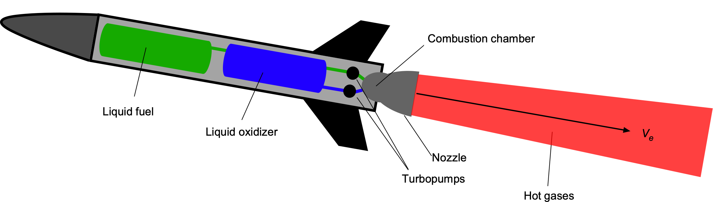
The thrust from a rocket motor follows directly from the conservation of momentum, i.e.,
(117) 
where  is the total propellant mass flow rate,
  is the exhaust or “jet” velocity,
  the nozzle exit pressure,
  the ambient pressure, and
  the exit area. It is convenient to define an effective exhaust velocity that absorbs the pressure term, i.e.,
(118) 
The specific impulse is then defined by
(119) 
The time taken, which serves as the canonical measure of rocket efficiency, is expressed in seconds. Notice that for a rocket,  can vary as it reaches higher altitudes above the Earth’s surface, so the mean sea-level (MSL) value,
  , is used.

For an ideal isentropic nozzle or “bell,” the exhaust velocity is obtained from the chamber stagnation conditions and the nozzle expansion ratio, i.e.,
(120) 
where  the chamber stagnation state, the ratio of specific heats, and
  the specific gas constant of the exhaust products. Lower values of molar mass increase the value of , leading to a higher speed of sound and greater exhaust velocity for a given
  . This is why hydrogen-oxygen propellants have superior performance compared with heavier hydrocarbon-oxygen systems.
The nozzle exit pressure is related to the area ratio  through the isentropic area-Mach relations, i.e.,
(121) ![\begin{equation*} \varepsilon = \frac{1}{M_e}\left[\frac{2}{\gamma+1} \left(1+\frac{\gamma-1}{2}M_e^2\right)\right]^{\tfrac{\gamma+1}{2(\gamma-1)}} \qquad \text{and} \qquad \frac{p_e}{p_c} = \left(1+\frac{\gamma-1}{2}M_e^2\right)^{-\frac{\gamma}{\gamma-1}} \end{equation*}](https://eaglepubs.erau.edu/app/uploads/quicklatex/quicklatex.com-0b6f8fa863cacd5a6091de4a7c9864ec_l3.svg "Rendered by QuickLaTeX.com")
The two aggregate performance parameters are the characteristic velocity and the thrust coefficient, which are given by
(122) 
This means that
(123) 
where  measures the combustion performance in the chamber and is independent of nozzle design, while
  measures the nozzle’s ability to convert the chamber’s pressure into thrust.
For an ideal equilibrium process, the value of depends only on the propellant chemistry, , and product properties. In practice, s is less than its theoretical value because of incomplete combustion, mixing limits, finite residence time, and chamber losses. The thrust coefficient , by contrast, reflects the effects of nozzle geometry and ambient pressure conditions, with MSL and vacuum values given by
(124) 
their difference dominated by the pressure-thrust contribution in and the chosen expansion ratio  .
.
The different rocket propulsion cycles are distinguished thermodynamically by how the turbopumps are powered and whether the turbine exhaust is returned to the main chamber. In the gas-generator cycle, a small fraction of the propellant is burned in a separate chamber to drive the turbopumps, and the turbine exhaust is discharged overboard. This arrangement is mechanically simple and reliable. However, some propellant energy is wasted, resulting in a lower specific impulse compared to closed cycles. To a first-order, a dump fraction imposes an  penalty.
In the staged-combustion cycle, a preburner operates at fuel-rich or oxidizer-rich conditions to generate turbine drive gas. After powering the turbopumps, this gas is fed into the main chamber, allowing all propellant to contribute to thrust. This architecture raises the effective chamber pressure, avoids dump losses, and yields higher values of and , and so higher values of , but at the cost of very demanding turbomachinery designs.
In the expander cycle, cryogenic fuel (usually liquid hydrogen) circulates through cooling channels around the chamber and nozzle, absorbing heat and vaporizing before driving the turbopumps and then entering the main chamber. This cycle is efficient and clean because no propellant is discarded. Still, it is thrust-limited by the available heat pickup, so the maximum  and chamber pressure are constrained by cooling power. A summary of these cycles is shown in the table below.
| Cycle | Pump drive/flow path | Advantages | Limitations | Typical applications | Indicative (sea-level/vacuum) |
|---|---|---|---|---|---|
| Gas-generator | A small propellant fraction burns in a gas generator → drives turbine → exhaust dumped overboard; remaining flow to main chamber → nozzle. | Simple, robust, good throttle response, high thrust-to-weight. | Energy discarded in turbine exhaust; lower than closed cycles. |
First stages & boosters where simplicity and  are prioritized. are prioritized. |
LOX/RP-1: 260–300 s / 300–330 s; LOX/LH : 360–380 s / ~430–445 s. : 360–380 s / ~430–445 s. |
| Staged-combustion | Preburner (fuel-rich or oxidizer-rich) drives turbine; turbine exhaust routed to main chamber so all mass expands through nozzle. | High , high chamber pressure  , good propellant utilization. , good propellant utilization. |
Complex, high stresses/temperatures, demanding materials & controls. | Reusable boosters, high-performance cores, and upper stages. | LOX/RP-1: 290–315 s / 330–360 s; LOX/LH: 375–395 s / 450–465 s. |
| Expander | Cryogenic fuel heated in cooling channels → drives turbine → enters main chamber; oxidizer pumped to chamber → nozzle. | Clean turbine drive, high efficiency, excellent reliability. | Thrust limited by available heat pickup; typically LH only. |
Cryogenic upper stages, long-duration restarts, precise orbital work. | LOX/LH: 360–380 s / 440–465 s (thrust typically modest). |
In practice, gas-generator rocket cycles are widely used in large launch vehicles where simplicity and high thrust-to-weight ratio are essential. Staged-combustion cycles predominate in modern high-performance boosters and upper stages, where the maximum efficiency is crucial for optimal performance. Expander cycles are primarily used in cryogenic upper-stage engines, where hydrogen is available and precise orbital maneuvers are required. However, all cycles reflect the same thermodynamic principles but represent different trade-offs among engineering simplicity, efficiency, and thrust production capability.
Check Your Understanding #5 – Rocket nozzle performance
 = 3, chamber (stagnation) temperature = 3,000 K, chamber pressure = 2.0
 Pa, ambient pressure = 1.0
 Pa , specific heat ratio = 1.2, and molar mass = 33.4 kg/mol. Assume isentropic expansion to the exit. Find the thrust per unit throat area
  and the specific impulse . (Question adapted from Engineering Thermodynamics, Work, & Heat Transfer by Rogers & Mayhew, 1980.)
Show solution/hide solution.
Compute the specific gas constant, i.e.,
![\[ R = \frac{R_u}{M} = \frac{8.314\times10^{3}~\mathrm{J/(mol\, K)}}{33.4~\mathrm{kg/mol}} = 2.49\times10^{2}~\mathrm{J/(kg\, K)} \]](https://eaglepubs.erau.edu/app/uploads/quicklatex/quicklatex.com-3b2ae52bbd0c7b9eaedb6ea6d839bb9b_l3.svg "Rendered by QuickLaTeX.com")
Solving the isentropic area-Mach number relationship for the exit Mach number (supersonic branch) gives
![\[ \frac{A_e}{A_t} = \frac{1}{M_e}\left( \frac{2}{\gamma+1}\!\left(1+\frac{\gamma-1}{2}M_e^2\right)\right)^{\tfrac{\gamma+1}{2(\gamma-1)}} = 3 \;\Longrightarrow\; M_e = 2.40 \]](https://eaglepubs.erau.edu/app/uploads/quicklatex/quicklatex.com-cff21ee34c5b6dba18a822016cd21b24_l3.svg "Rendered by QuickLaTeX.com")
The exit static temperature and pressure are
![\[ \frac{T_e}{T_0} = \frac{1}{1+\frac{\gamma-1}{2}M_e^2} \;\Longrightarrow\; T_e \approx 1.91\times10^{3}~\mathrm{K} \]](https://eaglepubs.erau.edu/app/uploads/quicklatex/quicklatex.com-2fa8461d15490931dbe35d1c72fcb978_l3.svg "Rendered by QuickLaTeX.com")
and
![\[ \frac{p_e}{p_0} =\left(\frac{T_e}{T_0}\right)^{\,\gamma/(\gamma-1)} \;\Longrightarrow\; p_e \approx 1.31\times10^{5}~\mathrm{Pa} \]](https://eaglepubs.erau.edu/app/uploads/quicklatex/quicklatex.com-24183824c313ba5e4c2895ddb7c9d56d_l3.svg "Rendered by QuickLaTeX.com")
The exit velocity is computed using  , where
  , i.e.,
![\[ V_e = M_e\sqrt{\gamma R T_e} = 1.81\times10^{3}~\mathrm{m/s} \]](https://eaglepubs.erau.edu/app/uploads/quicklatex/quicklatex.com-1523329445ce5b7cd44c198c7e24769a_l3.svg "Rendered by QuickLaTeX.com")
The choked mass flux at the throat is
![\[ \frac{\overbigdot{m}}{A_t} = \frac{p_0}{\sqrt{T_0}}\sqrt{\frac{\gamma}{R}} \left(\frac{2}{\gamma+1}\right)^{\tfrac{\gamma+1}{2(\gamma-1)}} = 1.50\times10^{3}~\mathrm{kg\,(s\, m^2)^{-1}} \]](https://eaglepubs.erau.edu/app/uploads/quicklatex/quicklatex.com-d6b9e41edf8d024542fee5054a262e42_l3.svg "Rendered by QuickLaTeX.com")
The thrust per unit throat area (momentum plus pressure thrust) is
![\[ \frac{F}{A_t} = \left(\frac{\overbigdot{m}}{A_t}\right) V_e + (p_e-p_a)\,\frac{A_e}{A_t} \]](https://eaglepubs.erau.edu/app/uploads/quicklatex/quicklatex.com-a909e687e3e159a510e78e8f8e69d6e2_l3.svg "Rendered by QuickLaTeX.com")
and so
![\[ \frac{F}{A_t} = (1.50\times10^{3})(1.81\times10^{3}) + (1.31\times10^{5}-1.00\times10^{5})\, 3 = 2.81\times10^{6}~\mathrm{N/m^2} \]](https://eaglepubs.erau.edu/app/uploads/quicklatex/quicklatex.com-5bbca5c4bd695c8bd0483ceec8b9f190_l3.svg "Rendered by QuickLaTeX.com")
Computing the specific impulse at  gives
gives
![\[ I_{\rm sp} = \frac{F/A_t}{(\overbigdot{m}/A_t)\,g_0} = \frac{2.81\times10^{6}}{(1.50\times10^{3})(9.80665)} = 1.91\times10^{2}~\mathrm{s} \]](https://eaglepubs.erau.edu/app/uploads/quicklatex/quicklatex.com-457428b10e429365cb89d6d080f39c29_l3.svg "Rendered by QuickLaTeX.com")
Thermodynamics of Combustion Processes
Combustion is the process by which stored chemical energy in fuels is released and converted into thermal energy. Heat addition raises the enthalpy of the working fluid, providing the power to drive pistons and turbines, and creating the thrust from rocket nozzles. Combustion, therefore, is the critical step that connects stored fuel energy to useful work and propulsion. In all applications, the principle remains the same: the combustion process establishes the thermal state of the working fluid, while the thermodynamic cycle or nozzle expansion determines how much energy can be extracted and converted into useful work.
From a thermodynamic perspective, combustion is the transformation of chemical bond energy into the enthalpy of the gaseous products, which is governed by the First Law and constrained by the Second Law through the principles of irreversibility and entropy generation. Fuels provide the potential, the chemical equations define the stoichiometry, and the thermodynamic laws determine how effectively that energy can be harnessed. For aerospace applications, the process must occur rapidly, reliably, and with high power density under widely varying conditions of pressure and temperature. This framework forms the basis for analyzing fuels, reaction equations, mixture ratios, and the efficiency of combustion in all types of engines.
Fuels
A combustion analysis begins with the fuel because its chemical composition determines the amount of energy available, the stoichiometric requirements, and the nature of the products. Aviation fuels are almost always hydrocarbons, chosen for their high specific energy and ease of handling and storage.
Aviation gasoline, 100LL, as used in piston engines, may be approximated by  and has a lower heating value (LHV) of about 44 MJ/kg. Kerosene-based fuels such as Jet-A (a kerosene) or RP-1 (densified kerosene = rocket propellant), commonly represented by
  , provide nearly the same energy content but with a higher density, which improves volumetric storage efficiency. These fuels are liquid at ambient conditions and can be stored and pumped using relatively simple mechanical systems, which explains their ubiquity in aircraft and rockets.
Hydrogen as a fuel is also of great importance in aerospace applications, particularly in high-performance rocket propulsion and experimental aeropropulsion applications. With an LHV of 120 MJ/kg, it offers more than double the energy per unit mass of hydrocarbons; however, its extremely low density (71 kg/m in liquid form) poses significant challenges for storage and tankage. Cryogenic handling is essential, but the high specific impulse achievable with liquid hydrogen (LH) and liquid oxygen (LOX) for rockets remains unmatched by any other propellant.
The choice of oxidizer is equally essential. Air serves as the oxidizer for air-breathing piston engines and gas turbines, maximizing the energy release from the fuel through the available oxygen content. Rockets, in contrast, must carry their oxidizer, with LOX being the most widely used. Alternative oxidizers, such as nitrous oxide or hydrogen peroxide, are used in specialized systems but have lower thermodynamic performance.
Chemical Equations – Conservation of Mass
Combustion can be expressed in the form of balanced chemical equations, which enforce the conservation of mass for each element. A hydrocarbon fuel  reacting with oxygen from the air serves as the general case. If the oxidizer is modeled as a mixture of oxygen and nitrogen in the ratio 1 : 3.76, then the stoichiometric reaction is written as
(125) 
The coefficient  is the stoichiometric coefficient, which is the number of oxygen molecules required per molecule of fuel and is determined by balancing the oxygen atoms, i.e.
(126) 
This expression ensures that every carbon atom appears in a carbon dioxide molecule and every hydrogen atom in a water molecule, while nitrogen remains unchanged as an inert diluent. Notice that the conservation of mass principle is satisfied automatically because the total number of atoms of each element is the same on both sides of the equation. In practical terms, this balance determines the minimum oxygen (and, therefore, the minimum air) required for the complete combustion of a given fuel.
By establishing such equations, the chemical nature of the fuel is connected with the thermodynamic description of combustion. The balanced reaction provides both the composition of the products and the precise fuel-oxidizer ratio at which all reactants are consumed. These relations form the foundation for defining stoichiometry, equivalence ratio, and the enthalpy liberated from the reaction of the fuel.
First Law Applied to Combustion
The balanced chemical equation establishes the composition of reactants and products. Still, thermodynamics is required to connect this reaction to the level of heat release that drives the engine and the propulsion. For example, in an adiabatic combustor with no shaft work, the First Law states that the chemical energy liberated during the breaking and reforming of chemical bonds appears as an enthalpy rise of the products.
If the reactants enter at a reference state (i.e., and ) and the products leave at the adiabatic flame temperature of  , the energy balance is written as
(127) 
where  is called the standard enthalpy of reaction obtained from the heats of formation, and
  is the specific enthalpy of species
  at a temperature . Expanding
  in terms of the temperature-dependent specific heats gives
(128) 
which defines the value of . For hydrocarbon fuels burning stoichiometrically in air, then is typically in the range of 2,200–2,500 K. This increase in energy content is the source from which turbines derive shaft power and nozzles generate thrust.
At high flame temperatures, however, a dissociation of  and
and  occurs, absorbing part of the energy and lowering both the equilibrium flame temperature and the effective ratio of specific heats, . This effect is significant in rocket combustion chambers and turbine combustors because it reduces the ideal work that can be extracted from the hot gases.
Combustion Efficiency
The combustion efficiency and pressure loss together describe how much of the fuel’s chemical energy is converted into a useful enthalpy rise of the working fluid and how much is dissipated through irreversibility. These quantities are critical inputs when assessing the performance of engines in a cycle analysis.
The First Law establishes the theoretical enthalpy rise available from a fuel, but the process is never ideal. Real combustors lose part of the chemical energy through incomplete burning, imperfect mixing, finite reaction rates, and heat transfer to the walls of the combustor. These departures from the ideal can be quantified by the combustion efficiency, defined as
(129) 
A value of  would correspond to complete conversion of the fuel’s LHV into the enthalpy of the products. In practical gas turbines, values of = 0.95–0.99 are achieved under steady operation, while rockets approach similar efficiencies through intense mixing in high-pressure chambers. Piston engines generally operate at slightly lower efficiencies because of cycle-to-cycle variability and flame quenching near the cylinder walls.
Another important practical measure is the total pressure loss across the combustor, which is usually expressed as
(130) 
where  is the total pressure at combustor entry and
  at the entry to the turbine. This drop reflects the irreversibility of the process because entropy is generated by chemical reactions, turbulent mixing, and heat transfer; thus, even if nearly all the fuel is burned, some of the pressure-producing potential is always lost.
Aerospace Applications
In gas turbines, combustion adds heat to the Brayton cycle. The process is at nearly constant pressure, so the required enthalpy sets the fuel-air ratio rise across the combustor, i.e.,
(131) 
where  is the compressor exit temperature and
  the turbine inlet temperature. The turbine must then supply enough work to drive the compressor; the BWR (as previously explained) makes the combustor performance central to the overall cycle in that the maximum attainable value of , which is limited by cooling and materials, fixes both the net specific work and the thermal efficiency. Modern high-bypass turbofans, turboshafts, and turbojets all rely on this balance, which in turn is controlled by how effectively combustion delivers the enthalpy rise without excessive pressure losses.
In rocket engines, the combustor sets the chamber temperature and the composition of the hot gases that expand through the nozzle. For a given mixture ratio  , the First Law defines the limiting value of through the adiabatic balance, while the exhaust exit velocity follows from nozzle thermodynamics, i.e.,
(132) 
The specific impulse, as given by
(133) 
is the key performance metric here, directly showing how the chemical energy is converted into thrust. A convenient decomposition of this uses the characteristic velocity  , defined by
(134) 
together with the thrust coefficient  so that
  . The mixture ratio controls and, therefore, the value of , while the nozzle design governs the value of .
Check Your Understanding #6 – Jet-A combustion
Approximate Jet-A as . (a) Write the balanced stoichiometric reaction with air modeled as  . (b) Compute the stoichiometric air-fuel ratio (AFR) by mass. (c) If a gas-turbine combustor operates with
  = 0.022 kg of fuel per kg of air, compute the equivalence ratio .
Show solution/hide solution.
(a) The general form of the combustion equation is fuel + oxygen → products. For Jet-A, then
![\[ \mathrm{C}_{12}\mathrm{H}_{23} + \nu_s(\mathrm{O_2}+3.76\,\mathrm{N_2}) \;\rightarrow\; 12\,\mathrm{CO_2} + \frac{23}{2}\,\mathrm{H_2O} + 3.76\,\nu_s\,\mathrm{N_2} \]](https://eaglepubs.erau.edu/app/uploads/quicklatex/quicklatex.com-18e9e06368199b9503c7af06cfc9764c_l3.svg "Rendered by QuickLaTeX.com")
Balancing oxygen gives 
(b) The fuel molar mass is  . Using
  = 32 and
  =28 gives
![\[ \mathrm{AFR}_{\rm st} = \frac{17.75\,(32+3.76\cdot 28)}{167} \approx 15.3 \]](https://eaglepubs.erau.edu/app/uploads/quicklatex/quicklatex.com-7240d2e143b63ca562fd68d96bcc05b4_l3.svg "Rendered by QuickLaTeX.com")
Approximately 15.3 kg of air is required for every 1 kg of Jet-A fuel.
(c) The actual fuel-air ratio is  . The equivalence ratio is
![\[ \phi = \frac{F/A}{(F/A)_{\rm st}} = f \, \mathrm{AFR}_{\rm st} = 0.022 \times 15.3 \approx 0.34 \]](https://eaglepubs.erau.edu/app/uploads/quicklatex/quicklatex.com-ee708456dda459b516974c2cbc88b1e8_l3.svg "Rendered by QuickLaTeX.com")
This result indicates lean operation, typical of a gas turbine.
Statistical Thermodynamics
Classical thermodynamics establishes relationships between macroscopic properties, such as pressure, temperature, internal energy, and entropy, but it does not explain why these relationships exist. Statistical thermodynamics (often referred to as statistical mechanics) provides the microscopic foundation of thermodynamics by connecting the observable, macroscopic behavior of matter to the motions and interactions of individual molecules.
Statistical thermodynamics not only explains the origin of the laws of classical thermodynamics but also extends them to conditions where molecular details matter, such as in hypersonic flows. At hypersonic speeds, the flow conditions are so extreme that the microscopic details of how molecules move, rotate, vibrate, and even dissociate govern the macroscopic flow. Statistical thermodynamics allows the calculation of heat capacities, equation of state relations, chemical equilibria, phase transitions, and even quantum effects. In this way, it provides the essential bridge between atomic physics and the macroscopic engineering applications of thermodynamics.
A microstate is a complete specification of the positions and velocities of all the particles in a system described by bulk variables such as , , and . Many different microstates can correspond to the same macrostate. The central idea of statistical thermodynamics is that the probability of a macrostate is determined by the number of microstates consistent with it. The microscopic interpretation of entropy is given by Boltzmann’s relation, i.e.,
(135) 
where is the entropy,  is Boltzmann’s constant, and
  is the number of accessible microstates compatible with the macrostate. Entropy, for example, has a clear probabilistic meaning, which states that states with more microstates are more probable, as illustrated in the figure below.
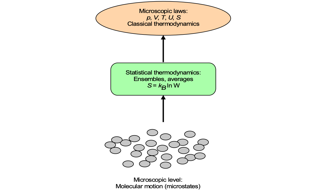
To make practical calculations, statistical thermodynamics introduces the concept of an ensemble, i.e., a large collection of identical systems, each representing a possible microstate. Depending on the constraints, different ensembles are used. In the microcanonical ensemble, the energy, volume, and particle number are fixed. In the canonical ensemble, the system exchanges energy with a heat reservoir, allowing the temperature, volume, and particle number to be fixed.
In the grand canonical ensemble, the system may exchange both energy and particles with a reservoir, and so the temperature, volume, and chemical potential remain fixed. Thermodynamic quantities then appear as ensemble averages. For example, the internal energy is expressed by
(136) 
where  is the energy of the microstate and
  is its probability.
Statistical thermodynamics shows that the familiar laws of thermodynamics are not arbitrary, but arise from the collective behavior of countless molecules. For aerospace engineering, the importance is both practical and theoretical. At everyday flight conditions, it explains why treating air as an ideal gas is sufficient. However, at the extreme conditions of high Mach number flight, reentry, and propulsion, it provides the only reliable way to account for changes in molecular energy storage, chemical reactions, and ionization. In this sense, statistical thermodynamics supplies the microscopic foundation needed to extend the field of classical thermodynamics to the realities of aerospace systems.
Check Your Understanding #6 – Specific heat of a diatomic gas
Why does the specific heat of air (comprised of N2 and O2), modeled as a diatomic gas, increase with temperature, and what representative values of , , and are expected at 300 K, 1,000 K, and 2,000 K?
Show solution/hide solution.
Statistical thermodynamics relates the molar specific heat at constant volume to the number of active molecular degrees of freedom, i.e.,
![\[ c_v = \frac{f}{2} R \qquad \text{and} \qquad R = 8.314~\mathrm{J/(mol\,K)} \]](https://eaglepubs.erau.edu/app/uploads/quicklatex/quicklatex.com-81fe3135aac02ac77b53c9d733d118fb_l3.svg "Rendered by QuickLaTeX.com")
For a diatomic gas, three translational and two rotational degrees of freedom are active, so = 5 and
![\[ c_v = \dfrac{5}{2}R = 20.8~\text{J/(mol K)}, \quad c_p = c_v + R = 29.1~\text{J/(mol K)}, \quad \gamma = \frac{c_p}{c_v} \approx 1.40 \]](https://eaglepubs.erau.edu/app/uploads/quicklatex/quicklatex.com-26f463ad59f137ed3a7ad617e267ebf1_l3.svg "Rendered by QuickLaTeX.com")
As the temperature rises, the vibrational modes become active, increasing the effective value of . Representative mixture-averaged values for air are then
![\[ \begin{aligned} T &= 300~\text{K}: & c_v &\approx 20.8, & c_p &\approx 29.1, & \gamma &\approx 1.40 \\ T &= 1000~\text{K}: & c_v &\approx 23.5, & c_p &\approx 31.8, & \gamma &\approx 1.35 \\ T &= 2000~\text{K}: & c_v &\approx 29.0, & c_p &\approx 37.0, & \gamma &\approx 1.28 \end{aligned} \]](https://eaglepubs.erau.edu/app/uploads/quicklatex/quicklatex.com-47e6cd25bf1edd74bb663e3a4f5831b1_l3.svg "Rendered by QuickLaTeX.com")
These results demonstrate how the vibrational excitation of N2 and O2 affects the thermodynamic properties of air, explaining why the assumption of constant specific heats is generally valid at most common flight conditions but inaccurate at the high temperatures associated with hypersonic flight.
Summary & Closure
This chapter has summarized the foundations of thermodynamics as they apply to aerospace systems. The definitions of systems, control volumes, and properties provide the framework for describing energy transfer through heat and work. Thermodynamic principles are often viewed as abstractions, but they are the basis for every aerospace component.
At its core, thermodynamics is just two simple truths: 1. Energy is conserved; it can change form (heat, work, motion, chemical energy), but it never disappears. 2. Energy spreads; left alone, useful, ordered energy (like motion or potential) always tends to become less useful and more disordered (entropy). Everything else, including enthalpy, entropy, free energy, and cycles, is a matter of careful bookkeeping based on those two fundamental ideas. To this end, the First Law of Thermodynamics states that energy is conserved, meaning it can change form but cannot be created or destroyed. The Second Law introduces the essential concept of the direction of energy flow and entropy, clarifying that not all energy transfers are equally useful and that irreversibility and exergy destruction impose unavoidable limits on performance.
In aerospace engineering, thermodynamics provides both a language and a set of limits. It explains what is possible, why 100% efficiency from an engine or other machine is unattainable, and how close designs can come to the theoretical ideal. Compressors and turbines embody the First Law as they exchange work with the fluid, while the Second Law governs their efficiency. Nozzles and diffusers illustrate how adiabatic flow preserves stagnation temperature but not stagnation pressure, emphasizing the impact of entropy generation. Combustors highlight the role of chemical energy conversion and the need to minimize irreversibilities in mixing and reaction. Even in rockets, where high chamber pressures drive dramatic expansions, the same laws define the maximum achievable thrust and specific impulse.
5-Question Self-Assessment Quickquiz
For Further Thought or Discussion
- What does the First Law of Thermodynamics imply about the conservation of energy in aerospace systems, and how does this principle constrain engine performance?
- How does the Second Law of Thermodynamics explain why no type of engine can be perfectly efficient, and how is this connected to entropy generation in propulsion devices?
- Why is the distinction between state functions (e.g., , , and ) and path functions ( and ) essential in analyzing thermodynamic cycles?
- In what ways does specific heat capacity reflect the molecular degrees of freedom of a gas, and why does this matter for air as the working fluid in propulsion?
- How do equations of state (such as the ideal gas law) simplify thermodynamic analysis, and under what conditions do real-gas effects become essential in aerospace?
- How do isobaric, isochoric, isothermal, and adiabatic processes differ in their heat and work interactions, and how are each represented on and diagrams?
- Why is the concept of reversibility central to defining the Carnot cycle, and how do irreversibilities appear in real aerospace engines?
- How does the ratio of specific heats influence isentropic relations, and why does this parameter strongly affect compressor and nozzle performance?
- How are enthalpy and stagnation enthalpy used to analyze flowing systems such as compressors, turbines, and nozzles in aerospace propulsion?
- Why is it useful to define efficiency metrics (thermal, propulsive, overall) in terms of energy balances, and how do these relate to the first and second laws?
Additional Online Resources
- Lecture 35: Otto Cycle, Diesel Cycle & Brayton Cycle (YouTube). A concise video covering the three primary power cycles with worked examples.
- Introduction to Otto, Diesel, and Brayton Cycles (YouTube). Elementary walkthrough of the key gas power cycles.
- Thermo Lesson 1 – Introduction to Thermodynamics (YouTube). A refresher on basic thermodynamic systems and principles.
- Otto, Diesel & Joule Cycles – GATE AE Lectures (YouTube). Formal lecture series with derivations useful for exam preparation.
- Thermodynamics: Review of Thermodynamic Cycles (YouTube). A good review with cycle diagrams and example problems.
- Gas Power Cycles – Purdue ME 200 Notes. Textbook-style PDF with derivations, diagrams, and worked problems on Otto and Diesel cycles.
- GATE Thermodynamics Full Course (YouTube playlist). Structured lecture series covering thermodynamic fundamentals and cycles.
- Propulsion Basics – GATE Aerospace Engineering Lectures (YouTube playlist). Course-style treatment with emphasis on aerospace propulsion thermodynamics.
- This chapter is based, in part, on lectures on thermodynamics by Professor Robert S. Silver (1913–1997) at the University of Glasgow, where he held the James Watt Chair of Mechanical Engineering & Thermodynamics. Professor Silver is best known for his work on the thermodynamics of irreversible processes and is considered the father of the modern desalination industry, for which he was recognized with the UNESCO Prize for Science. His textbook, An Introduction to Thermodynamics – with Some New Derivations Based on Real Irreversible Processes, remains a fundamental work in the field. ↵
- In thermodynamics, a reversible process is an idealized process in which both the system and its surroundings can be returned to their initial states by an infinitesimal change in some property of the surroundings (such as pressure, temperature, or an external field). ↵
- A transitive property means that if one quantity relates to a second, and the second relates to a third, then the first also relates to the third. ↵
- Experiments by Jean Baptiste Perrin led to the definition of the Avogadro number as the number of molecules in one gram-molecule of oxygen. Perrin named it Avogadro's number in honor of Amedeo Avogadro. Standardization of the SI system then led to the formal definition of the Avogadro constant. ↵
