B-3: Ideal Flow Analysis (1)
Fundamental Ideal (Potential) Flow Field Analysis (1 of 2)
Shigeo Hayashibara
What is potential flow Field?
Ideal (Potential) Flow Field
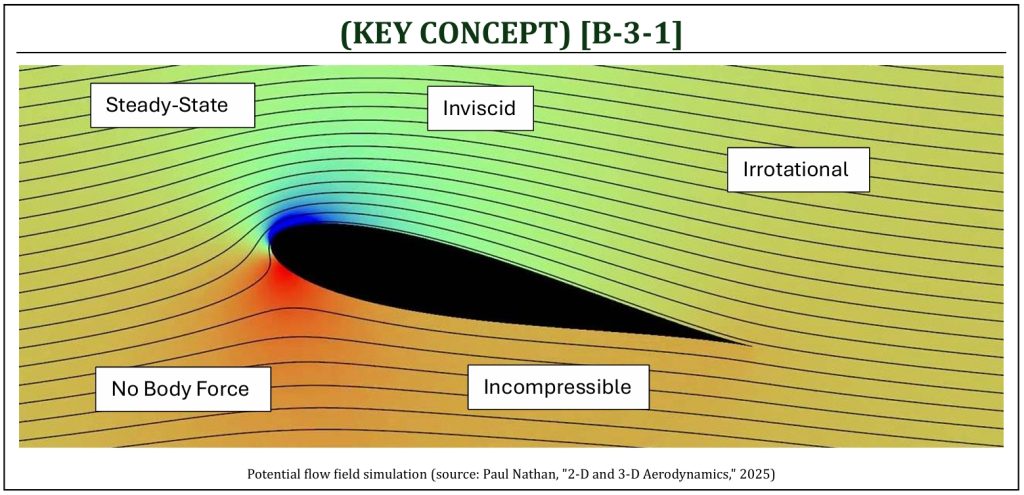
As a very fundamental analytical method in theoretical aerodynamics, we will first attempt to solve the governing equation, called Laplace’s equation, in some simple flow fields. This purely mathematical aerodynamic analysis of an ideal flow field is called, the “potential flow analysis.” In order to analytically solve the governing (Laplace’s) equation of a flow field, we need to apply the following assumptions to simplify the flow field equation.
(1) What are the assumptions made to simplify the equation (i.e., the condition for the Laplace’s equation to be valid to describe the flow field)?
-
Steady-state? The time-rate of change for the flow field is completely ignored. The flow field is independent of time.
-
Inviscid? The viscosity and associate effects (i.e., boundary layer) are all completely ignored.
-
No body force? The gravity is assumed to have no effect on the flow field. Also, there is no magnetic field (potentially alter the flow field) present.
-
Incompressible? The density of the flow field is assumed to be constant. The condition for this assumption to be true would usually be less than 0.3 Mach number (i.e., incompressible subsonic flow).
-
Irrotational? The viscosity induced internal strain (i.e., vorticity) is completely ignored.
(2) Because of the assumptions made, how your theoretical solution “different” (or apart) from the actual (or real) flow field phenomena?
-
The potential flow field analysis provides theoretical solution for the “ideal” flow field. This will establish fundamental flow field behavior. Due to the assumptions (limiting conditions), the solution does not accurately represent the “real” flow field.
-
Suppose . . . can we “model” those assumptions (limiting conditions) one at a time, separately. Then, can we “add-on” those results onto the “ideal” flow field solution? (the answer is “yes,” and this approach is commonly called, “Euler (or ideal flow) solution + BL + Compressibility Correction” flow field analysis).
Let us just summarize the “road map” (STEPS: 1 , 2, 3, and 4) of a fundamental potential flow analysis procedure.
Potential Flow Field Analysis
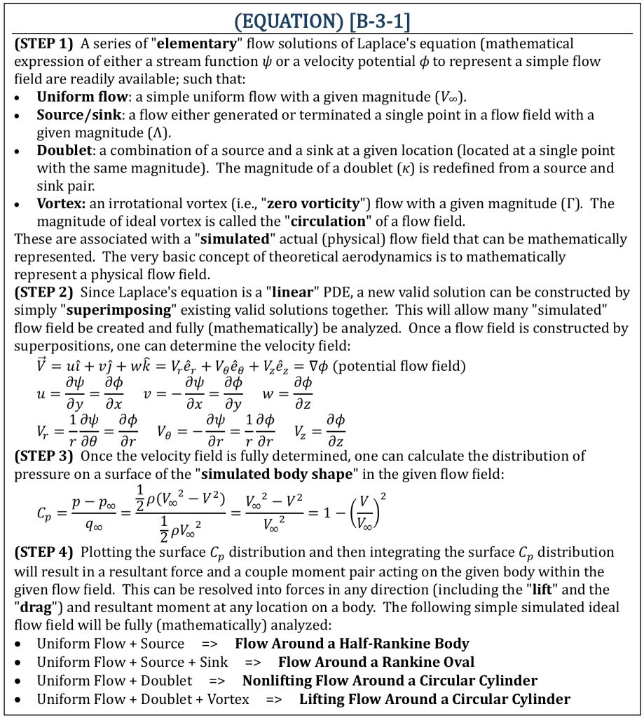
1st elementary flow solution of laplace’s equation: uniform flow
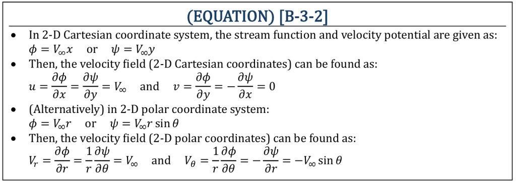
Uniform Flow
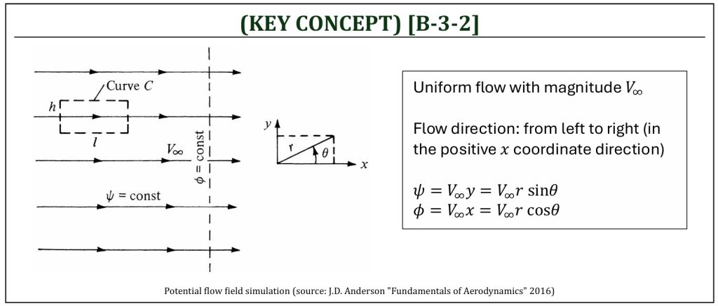
Uniform flow with magnitude V∞ and direction in positive x coordinate is the 1st elementary flow solution of Laplace’s equation. This can physically represent the uniform “freestream” of the flow field.
Uniform Flow
2nd elementary flow solution of laplace’s equation: source/sink
Source/Sink
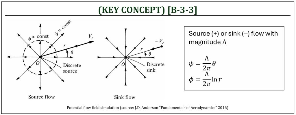
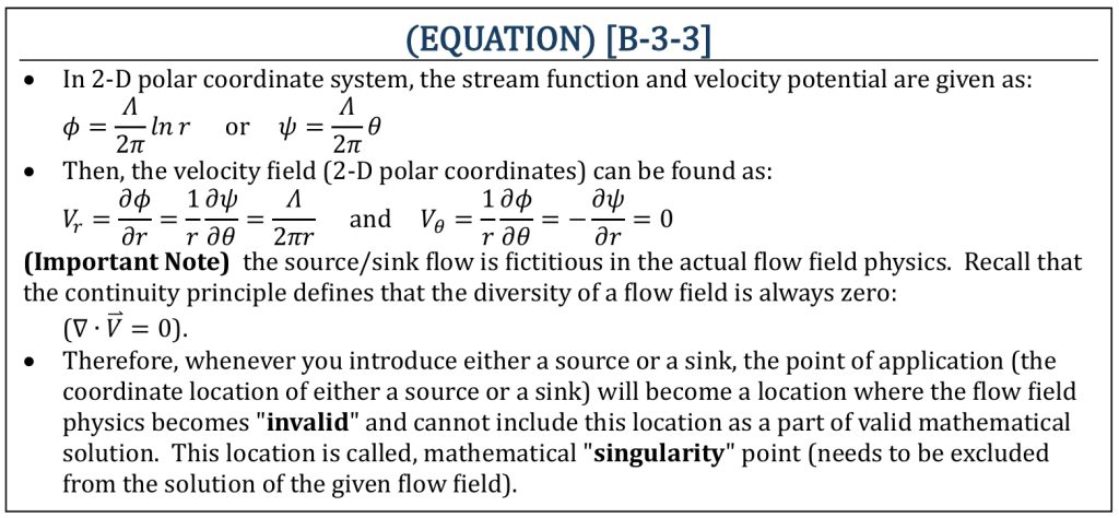
The source (+) / sink (-) flow is the 2nd elementary flow solution of Laplace’s equation. A sink/source flow can be characterized by a series of straight streamlines emanating from a single point. The strength of source/sink (Λ) can physically represent the volume flow rate (per unit depth).
Source/Sink
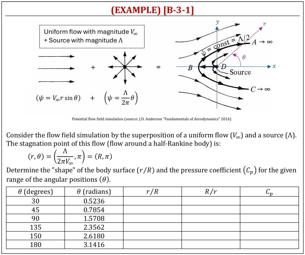
Superposition (1): uniform flow + source = Flow around a half-rankine body
Flow around a Half-Rankine Body
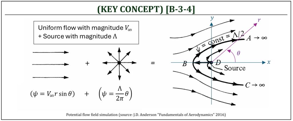
Combining two elementary flow solutions of Laplace’s equation (uniform flow + Source) will construct a simulated flow field around a semi-infinite body, called a “half-Rankine” body.
Flow around a Half-Rankine Body
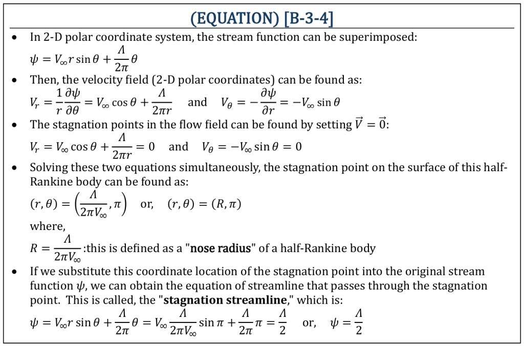
It is possible to draw any number of streamlines in the given flow field. However, the stagnation streamline is the one that defines the “shape” of the body in the flow field, if the stagnation point is located on the surface of the body. If it is so, the velocity and pressure distribution on the surface of the body can mathematically be calculated along this particular streamline (stagnation streamline).
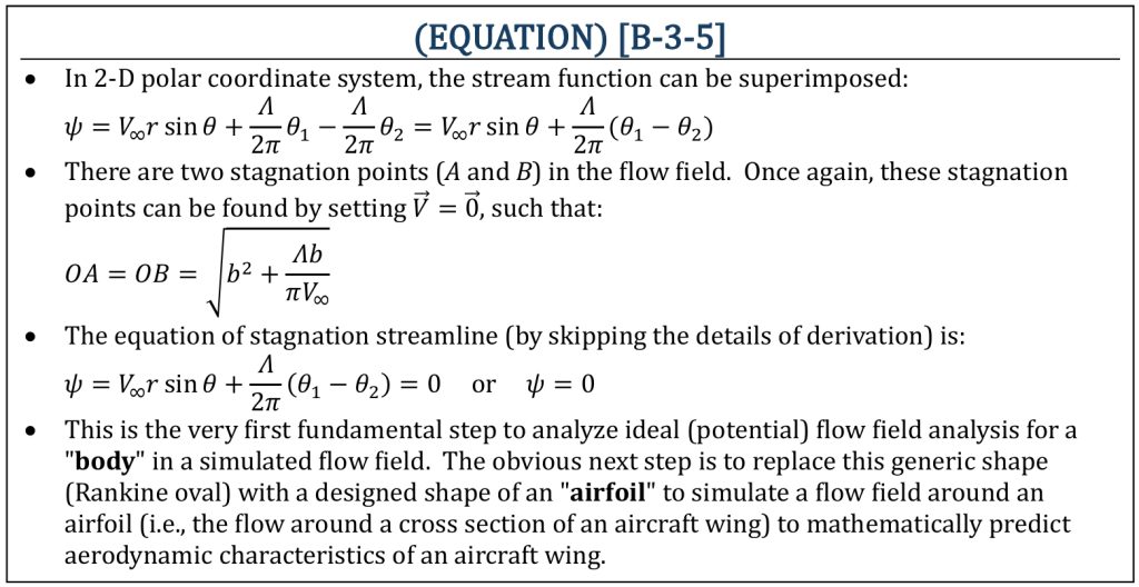
Superposition (2): uniform flow + source + SINK = Flow around a rankine Oval
Flow around a Rankine Oval
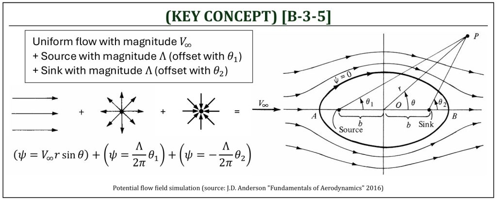
Combining three elementary flow solutions of Laplace’s equation (uniform flow + Source + sink) will construct a simulated flow around an oval, called a “Rankine” oval.
Flow around a Rankine Oval
Flow around a Half-Rankine Body
3rd elementary flow solution of laplace’s equation: doublet
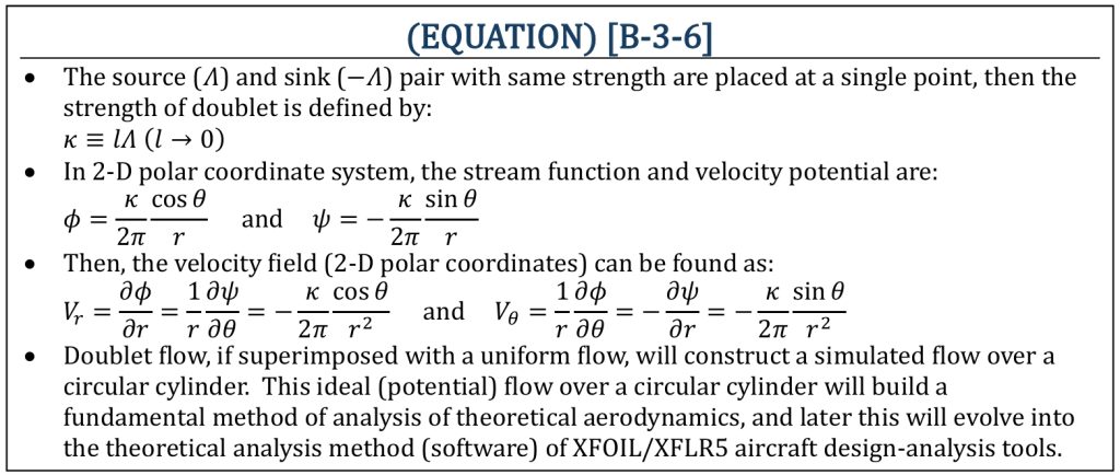
Doublet
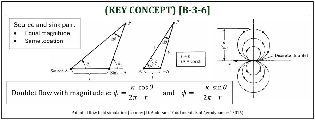
The doublet flow is the 3rd elementary flow solution of Laplace’s equation. The source (Λ) and sink (–Λ) pair with same strength at a single point can be defined as a doublet flow with a strength (κ).
Doublet
4th elementary flow solution of laplace’s equation: vortex
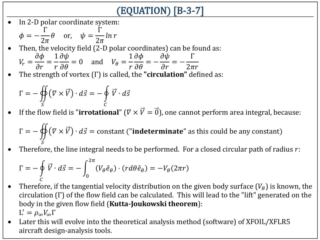
Vortex
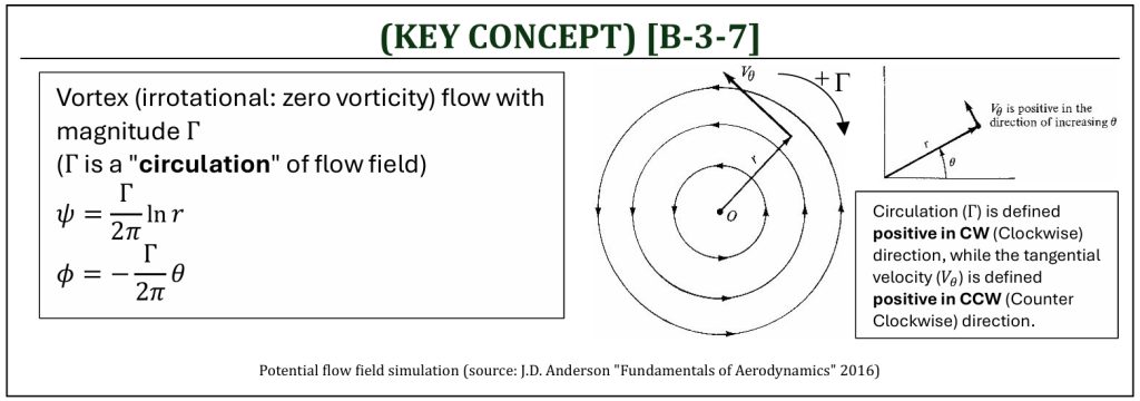
The vortex flow is the 4th elementary flow solution of Laplace’s equation. This simulates a flow field with a series of streamlines of concentric circles centered around a single point. The magnitude of vortex is the flow field “circulation,” that is going to generate a “lift” of a body in a uniform flow (Kutta-Joukowski theorem). It is important to understand that the ideal (potential) flow field is inviscid, so there is no “curl” (vorticity) in the given flow field. The name of the vortex often is misleading, because there is no vorticity for this vortex flow.
Vortex
uniform flow + Doublet = nonlifting flow over a circular cylinder
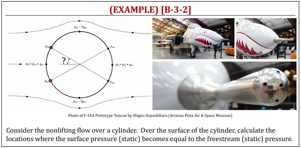
Nonlifting Flow over a Circular Cylinder
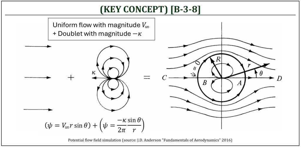
Combining two elementary flow solutions of Laplace’s equation (uniform flow + Doublet) will construct a simulated flow around a circular cylinder.
Nonlifting Flow over a Circular Cylinder
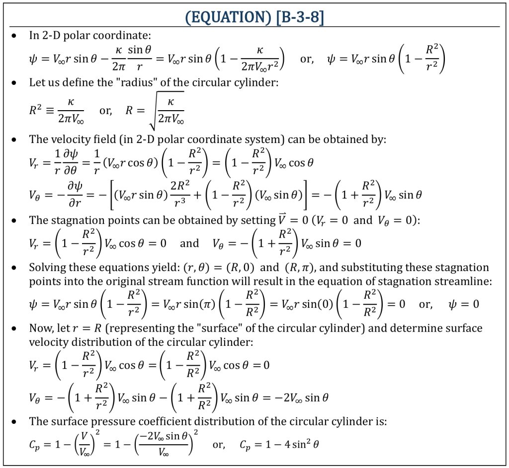
nonlifting flow over a circular cylinder
Pressure Distribution over the Surface of a Circular Cylinder
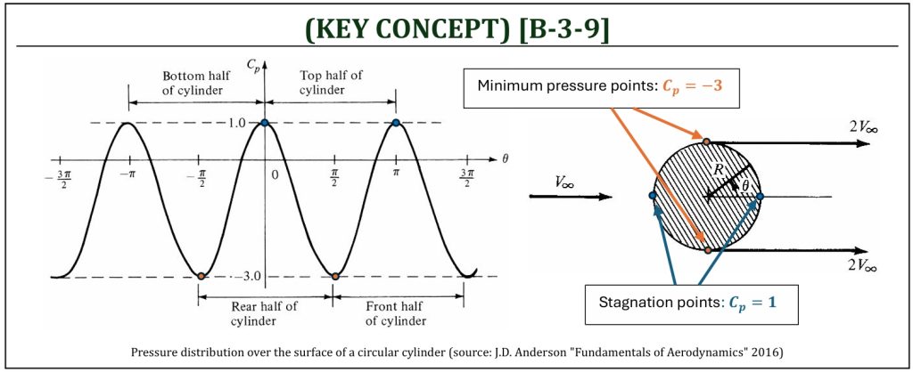
A close observation of the pressure coefficient distribution on the surface of the cylinder indicates some interesting behaviors. We must understand that this is purely mathematical analysis of an ideal (potential) flow field. We are ignoring the effects of viscosity.
d’Alembert’s Paradox
-
It is, actually, understandable that the flow over a circular cylinder does not generate aerodynamic “lift”. One interesting way to actually generate “lift” is “spinning” the cylinder (adding a circulation onto the given flow field).
-
The potential flow analysis does not include “viscosity” (irrotational flow), thus “drag” calculation requires a separate model (boundary layer analysis) to be added onto the potential flow analysis.
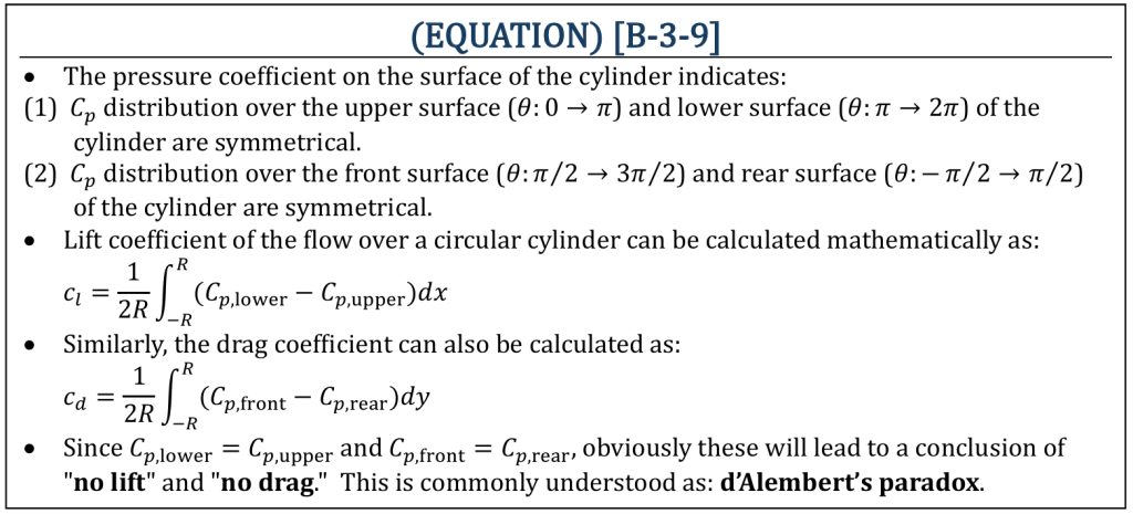
Although it is obviously predictable that the lift coefficient of the flow over a circular cylinder is zero (as there is no difference of pressure distribution between upper and lower surfaces), it is beneficial to mathematically calculate it at this moment. Once the pressure distributions between upper and lower surfaces become different, it will introduce an aerodynamic “lift.”
Aerodynamic Lift for Nonlifting Flow over a Circular Cylinder
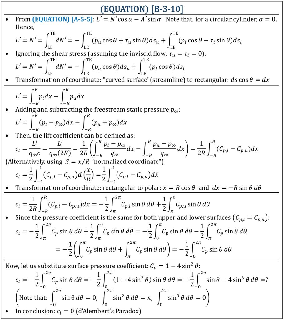
Pressure Distribution for Nonlifting Flow over a Circular Cylinder
Ideal v.s. real nonlifting flow over a circular cylinder
Viscos Effects for Nonlifting Flow over a Circular Cylinder
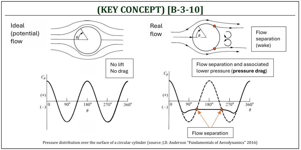
The pressure distribution around circular cylinder (ideal flow) is symmetric; thus “no lift” and “no drag” will be produced. This is known as d’ Alembert’s paradox of potential flow analysis. Flow separation, due to the adverse pressure gradient, and resulting complex wake region induces the non-symmetric pressure distribution, thus “drag due to flow separation” (often called the “pressure drag“) is the main drag contributor of real flows around a circular cylinder.
As it is obviously observed, the presence of viscosity will cause an aerodynamic drag. This is often called, “aerodynamic profile drag.” The name implies that the drag is caused by the presence and the behavior of the surface boundary layer (due to viscosity). For detailed analysis on an aircraft wing’s cross section (airfoil), the profile drag can further be categorized into the following two different types of drag components:
-
Skin Friction (or “parasite”) Drag is the aerodynamic profile drag, caused by “attached” boundary layer (surface friction due to shear stress). The actual amount of drag depends on flow type (either “laminar” or “turbulent” flow). Obviously, the turbulent flow is associated with higher friction than the laminar flow (remember “pipe flow analysis” in Fluid Mechanics).
-
Pressure Drag (or “drag due to flow separation”) is the aerodynamic profile drag, caused by “separated” boundary layer (due to pressure difference, caused by the flow separation).
real nonlifting flow over a circular cylinder (1): Reynolds Number
Real Flow over a Circular Cylinder
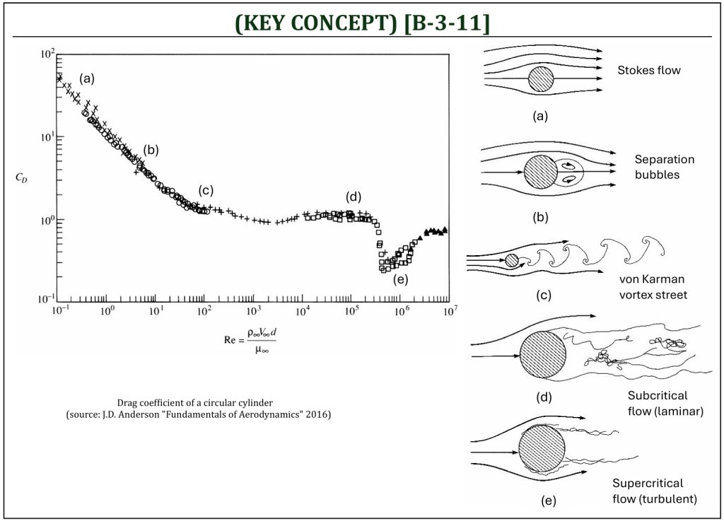
A real flow over a circular cylinder can be more complicated due to the presence of viscos effects. Let us examine some existing experimental results. Based on the flow field Reynolds number, we can categorize five distinctive flow field regimes:
(a)  : the pressure forces and the friction forces balance each other: similar to the ideal flow (Stokes flow). The flow field is very close to symmetrical.
  . The majority of drag in this flow regime is due to viscosity (i.e., the skin friction, or “parasite” drag).
(b)  : the flow is separated on the back of the cylinder forming two stable (attached) vortex bubbles (separation bubbles). The separation of the flow in the rearward face of the cylinder starts to occur, due to the adverse pressure gradient. The separation is close to steady state in this flow regime, maintaining two symmetrical separation “bubbles.”
  .
.
(c)  : the alternate shedding of vortices (von Karman vortex street) is observed (unsteady flow). As the Reynolds number is increased, the vortex street becomes turbulent and turns into a wake: the
  is nearly constant (
 ). The separation of the flow in the rearward face of the cylinder starts to become unsteady and separated from the surface.
  . The drag coefficient stays fairly constant over a wide range of Reynolds number, until the boundary layer transitions from laminar to turbulent (
 ).
).
(d)  : the separation of the laminar boundary layer takes place on the forward face of the cylinder (subcritical flow). The early flow separation (laminar flow) creates a large separation (“pressure”) drag.
(e)  : the boundary layer transition from laminar to turbulent flow occurs. As the Reynolds number is increased, the skin friction drag slightly increases but the reduction of flow separation (smaller wake region) dramatically decreases the pressure drag due to the flow separation (supercritical flow). The turbulent flow delays flow separation and reduces the separation (“pressure”) drag. Although the skin friction (“parasite”) drag will be increased slightly due to the flow transition from laminar to turbulent, overall total drag will be reduced.
real nonlifting flow over a circular cylinder (2): Boundary Layer Transition
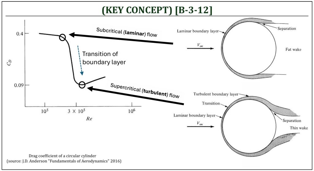
Subcritical v.s. Supercritical Flows
Although the skin friction (“parasite”) drag will be increased slightly due to the flow transition from laminar to turbulent, overall total drag will be reduced. The boundary layer transition control has been applied to develop efficient golf balls. The presence of surface dimples of golf balls induces transition from laminar to turbulent boundary layer and delays flow separation. As a result, the drag coefficient of a golf ball is reduced (aerodynamic drag of golf balls with dimples are lower than smooth ones).
-
Subcritical (laminar) flow: although the skin friction drag is smaller in laminar flow (smaller than the turbulent flow), the flow separation tends to occur at an early stage of the adverse pressure gradient region (thus, often induces a large pressure drag).
-
Supercritical (turbulent) flow: although the skin friction drag is larger than laminar flow, the flow separation moves aft (the turbulent flow tends to stay attached on the surface under the adverse pressure gradient). Thus, often the pressure drag is relatively small (smaller than the laminar flow).
References
- 2D & 3D Aerodynamics by P. Nathan (YouTube@PaulNathan82)
- Fundamentals of Aerodynamics by J.D. Anderson, 5th ED, McGraw Hill, 2016
- Aerodynamics for Engineers by J. J. Bertin & M. L. Smith, 3rd ED, Cambridge University Press, 1997
- Aerodynamics for Engineering Students by E. L. Houghton & P. W. Carpenter, 4th ED, Edward Arnold, London, 1993
Media Attributions
If a citation and/or attribution to a media (images and/or videos) is not given, then it is originally created for this book by the author, and the media can be assumed to be under CC BY-NC 4.0 (Creative Commons Attribution-NonCommercial 4.0 International) license. Public domain materials have been included in these attributions whenever possible. Every reasonable effort has been made to ensure that the attributions are comprehensive, accurate, and up-to-date. The Copyright Disclaimer under Section 107 of the Copyright Act of 1976 states that allowance is made for purposes such as teaching, scholarship, and research. Fair use is a use permitted by copyright statute. For any request for corrections and/or updates, please contact the author.
