C-1: Aerodynamics of Airfoils (1)
Aerodynamics of 2-D Airfoils (1 of 2)
Shigeo Hayashibara
Aircraft wings (3-D) and Airfoils (2-D)
Wings (3-D) and Airfoils (2-D)
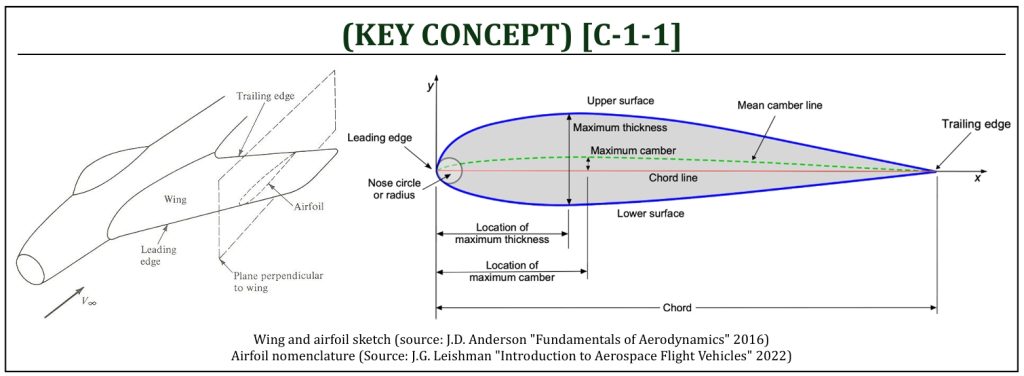
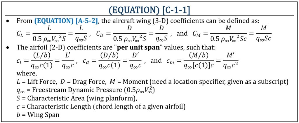
Recalling from A-5, the aircraft wing (3-D), as well as airfoil (2-D), coefficients of lift, drag, and pitching moment are defined in both upper case (3-D) and lower case (2-D) symbols. It is quite important to distinguish these differences. As we analyze and simulate aircraft performance, it usually starts from 2-D (airfoil) characteristics. The integrated effects of each and all airfoil (2-D) characteristics are the predicted wing (3-D) performance. It is important to carefully stay in “non-dimensional” coefficients throughout the analysis to maintain analytical size independence.
Wings (3-D) and Airfoil (2-D) Coefficients
Airfoils (1): Lift Curves
Lift Curves of Airfoils
The design of airfoil (2-D) will have a significant impact on aircraft wing (3-D) performance. Airfoils represent the performance of a given 2-D cross-section at each spanwise location of a 3-D wing. Since a wing is composed of a series of cross sections (i.e., airfoils) across the wing span, the shape of an airfoil (i.e., a characteristic performance at each spanwise cross-section) essentially determines the overall performance of a wing. The “shape” of airfoil (the design of 2-D airfoil) is essentially a control of a “pressure gradient.” The shape itself will have a significant impact on aircraft, depending on either “favorable” or “adverse” nature of the pressure gradient. Mathematically, the pressure gradient of a given flow field can be represented by EQUATION [B-1-3].
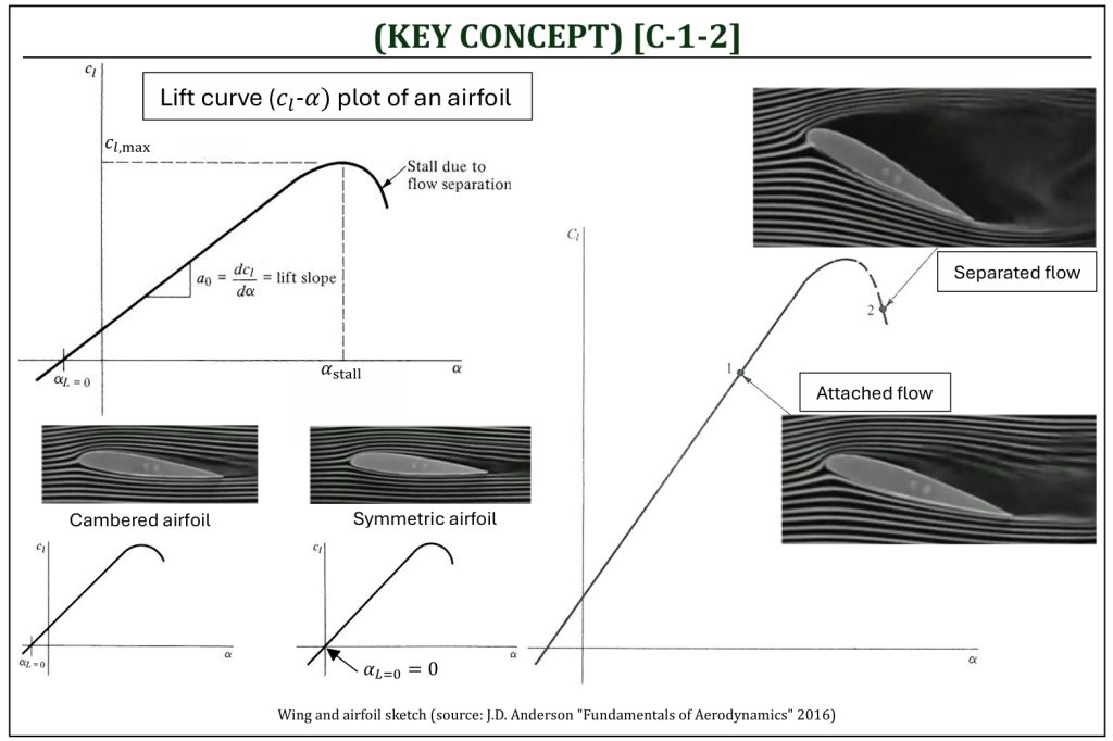
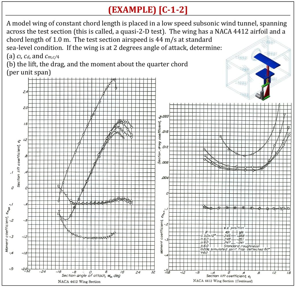
Airfoils represent the performance of a given cross-section of a wing. The shape of an airfoil determines fundamental behavior; thus, will have tremendous impacts on the overall performance of wing (i.e., aircraft performance). Airfoils can be considered as a simplified model for a “unit span” of an infinite wing of constant cross-section. The performance of an airfoil can be determined by a “quasi-2-D” wind tunnel test. A Quasi-2-D is, actually, a 3-D test with a constant cross section across the wing span. The cross-sectional (i.e., 2-D airfoil) properties (i.e., lift, drag, and moment “per unit span“) can be determined from this type of test. The behavior of lift (the “lift curve” characteristics) depends on the following properties:
-
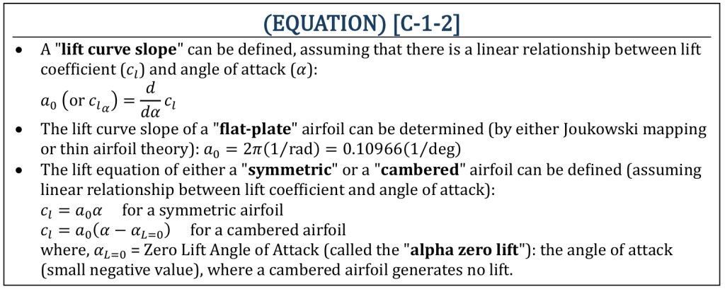
Angle of attack (α): the lift-curve provides important relationship between angle of attack (α) and lift coefficient (cl), under a certain condition of Reynolds number. Interestingly, lift-curve is fairly close to a linear line, as long as it is not under the “stall” condition (we often assume it is a simple linear function with a constant slope for simplification). The slope of this lift curve is called, “lift curve slope” (a0).
-
Viscus effects : the lift curve depends on the Reynolds number of the given flow field.
-
Freestream Mach number (i.e., “compressibility“): the lift curve will also depend on the compressibility of the flow field.
In order to “adjust” the wing aerodynamic characteristics, often the cross-section of a wing needs to be varied across the span (called, the “twist” of a wing). There are two categories for such adjustments:
-
Geometric twist of wing: varying angle of attack along the span but retains the same airfoil along the span.
-
Aerodynamic twist of wing: varying the type of airfoil (cross section of the wing) along the span but retains the same angle of attack along the span.
Airfoils (2): Camber
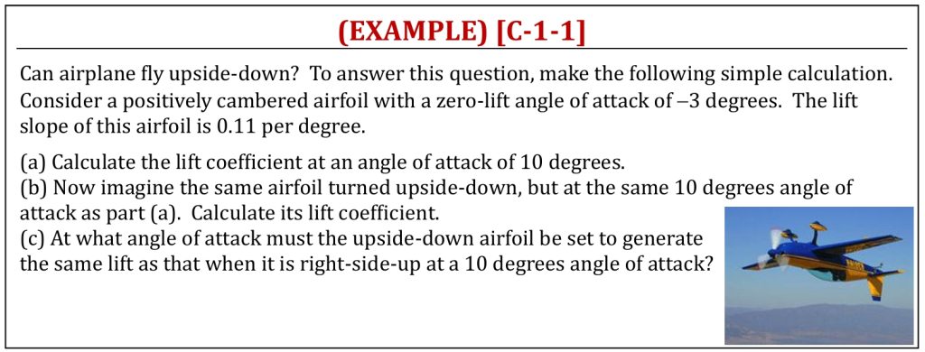
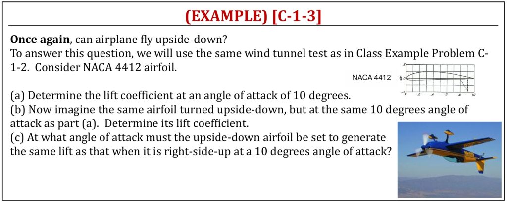
The camber in airfoil is the asymmetry between the top and the bottom surface curves of an airfoil. Cambered airfoils generate lift at positive, zero, or even small negative angle of attack, whereas a symmetric airfoil only has lift at positive angles of attack. It is important to note that the camber does not usually alter the lift curve slope (a0), but “shift” the entire curve either to “left” (where, the angle of attack for a zero lift αL=0 is “negative“) or “right” (where, αL=0 is “positive“). If αL=0 is negative, it is usually called the “positive” camber (i.e., enhances “lift“), while the other is called “negative” camber (i.e., enhances “down force“).
Lift of an Airfoil (Symmetric and Cambered)
Upside-Down Flight (1)
Airfoils (3): NACA Airfoils
NACA Airfoils
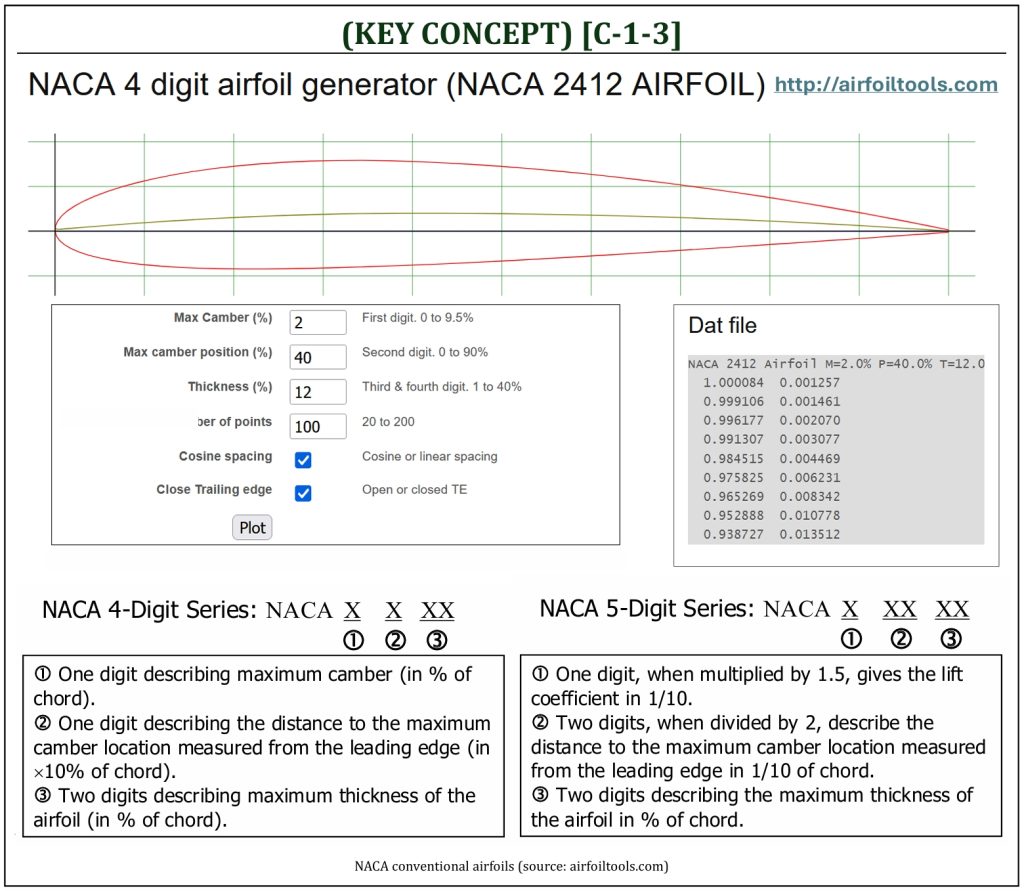
NACA airfoils are airfoil shapes developed by the National Advisory Committee for Aeronautics (i.e., predecessor of NASA: 1915-1958). The lift, drag, and moment coefficients for these airfoils were obtained through wind tunnel tests conducted in 1950s (summarized in NACA Report 824). The normalized coordinates (x/c and y/c) of NACA 4-digit or 5-digit series (these are commonly called, “NACA conventional airfoils“) can be mathematically computer-generated (NASA-96-TM4741). NACA conventional airfoils have maximum thickness (usually) at quarter chord location (c/4). For a conventional airfoil, the maximum thickness location is designed to be at the location of aerodynamic center (very close to the quarter chord location).
NACA Airfoil Data
If the maximum thickness location is moved (usually only toward “aft” not “forward”), the airfoil design is usually considered “non-conventional” (i.e., NACA 6-series Natural Laminar Flow or “NLF” airfoils). There are a few well-known NACA non-conventional airfoil series:
- NACA 1-Series: mathematically derived airfoil shape from the desired lift characteristics. Prior to this, airfoil shapes were only determined using a wind tunnel.
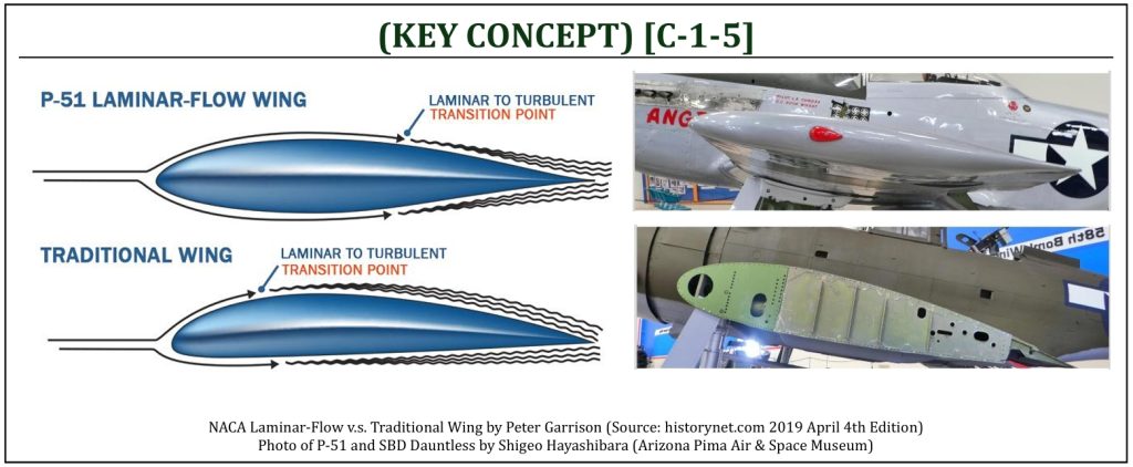
- NACA 6-series (Natural Laminar Flow, or “NLF” airfoil): an improvement over 1-series airfoils with emphasis on maximizing natural laminar flow (NLF). Maximum thickness is moved (close) to the half chord location.
- NACA 7-series: further advancement in maximizing laminar flow achieved by separately identifying the low pressure zones on upper and lower surfaces.
- NACA 8-series (NASA-Super Critical, or “NASA-SC” airfoil): supercritical (SC) airfoils designed to optimize transonic flow characteristics.
Airfoils (4): NACA 6-Series Airfoils
NACA 6-Series Natural Laminar Flow (NLF) Airfoils
There is a unique development of NACA airfoil in 1940-1950’s with a strong emphasis on maximizing the laminar flow on the surface of an airfoil. This is called, “Natural Laminar Flow” (NLF) airfoil (NACA 6-series). The airfoil is described in 6-digit designation in the following sequence:
- The number “6” indicating the series (NACA 6-series NLF airfoil).
- One-digit describing the distance of the minimum pressure point in tens of percent (×10%) of chord.
- One-subscript(or parentheses)-digit describing that the range of lift coefficient in tenths (1/10) above and below the design lift coefficient in which favorable pressure gradient exist on both surfaces (range of low drag maintained).
- A hyphen inserted.
- One-digit describing the design lift coefficient at zero angle of attack in tenths (1/10).
- Two-digits describing the maximum thickness in percent of chord.
For example, NACA 622-315 or NACA 62(2)-315 describes a NACA 6-series (NLF) airfoil with the point of minimum pressure 20% of the chord, maintains low drag 0.2 above and below the lift coefficient of 0.3, and the maximum thickness of 15% of the chord. The North American XP-51 (Mustang) was the very first aircraft to design incorporate a NACA 6-series (NLF) airfoil. Many variants of NACA 6-series (NLF) airfoil have been widely adapted since this extremely successful WWII aircraft design. Comparing against conventional NACA 4-digit or 5-digit airfoils, NACA 6-series (NLF) airfoils significantly reduce the cruising skin friction drag under a certain (typically a “cruising“) flight condition, leading to a longer range and endurance of an aircraft.
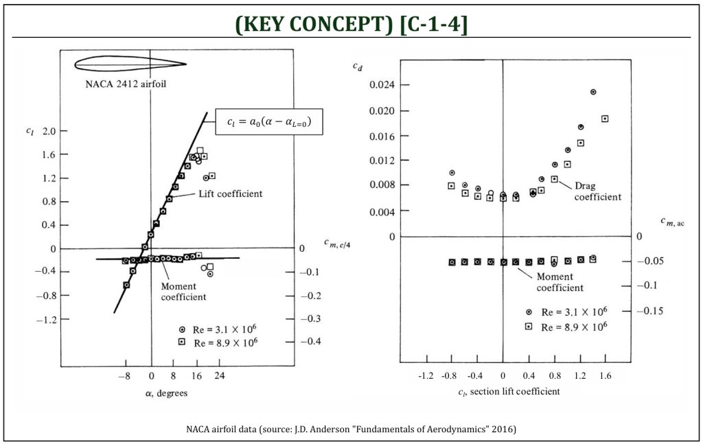
NACA airfoils typically have complete data of lift and moment diagram. This shows the change in lift coefficient, drag coefficient, and pitching moment with angle of attack. There is also typically a plot of lift coefficient against drag coefficient, called the “drag polar” diagram, which gives the analytical database (required thrust for a propulsion system) for flight mechanics (i.e., flight performance).
Quasi 2-D Wind Tunnel Test
Upside-Down Flight (2)
Pressure Coefficient distributions of an airfoil
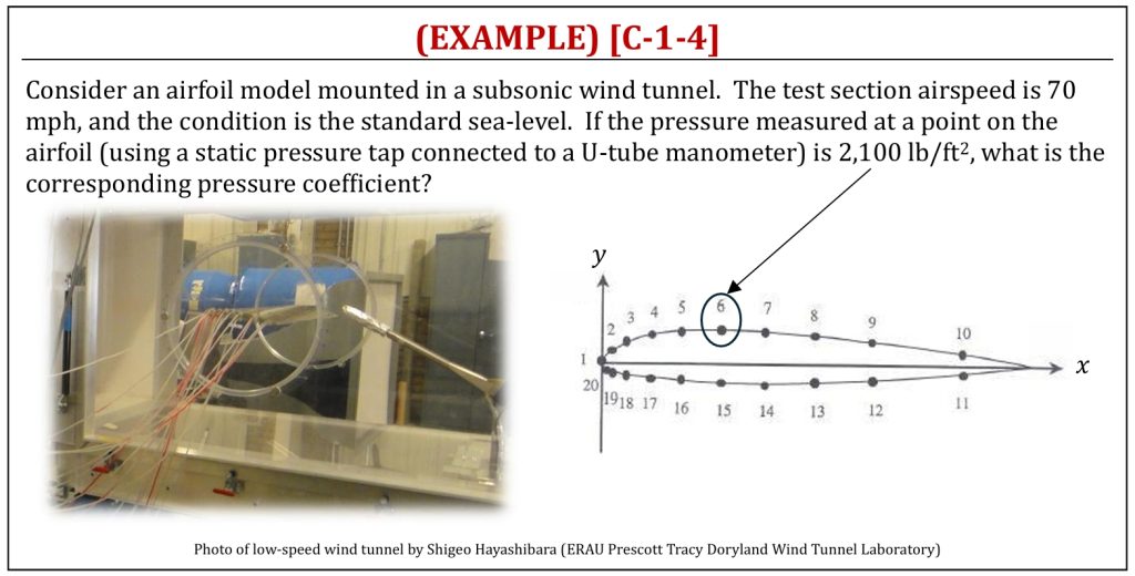
Pressure and Lift Coefficients
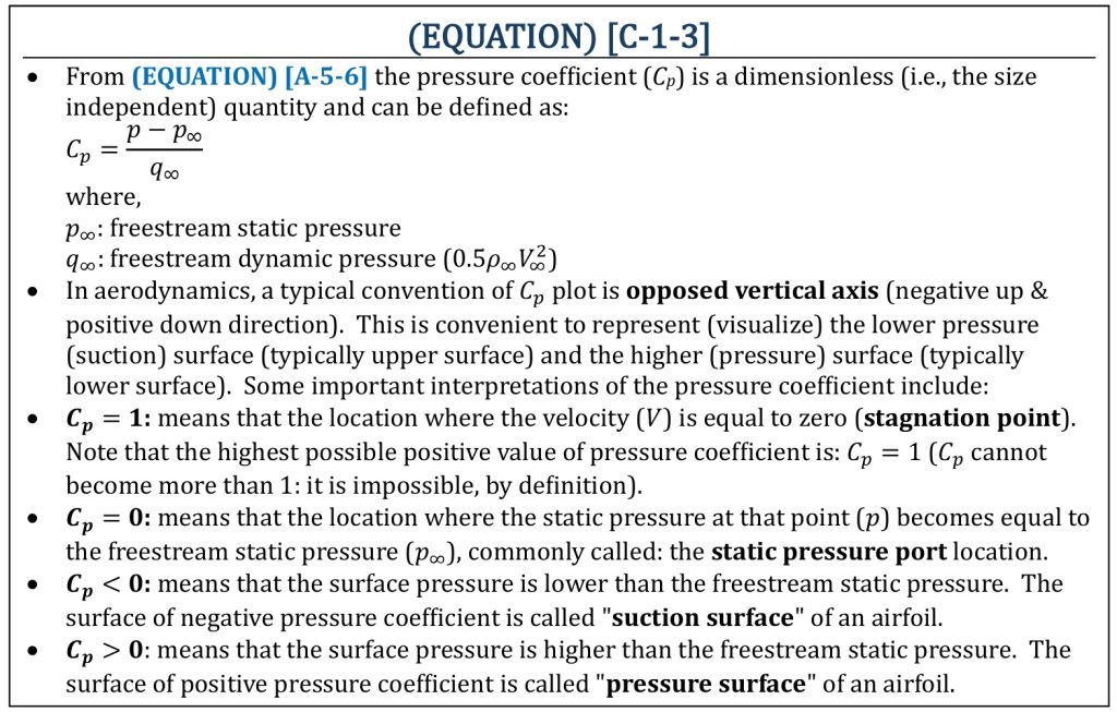
Let us review EQUATION [A-5-4] and EQUATION [A-5-5] one more time. Let us simplify the equation by letting inviscid (zero shear stress). The surface (i.e., upper and lower surfaces) pressure distributions can be integrated to obtain a lift per unit span. Instead of pressure itself, we should choose “pressure coefficient” (Cp) distributions on the surface of an airfoil. Also, instead of coordinate itself, we should choose “normalized coordinate” for analysis. The purpose here is to perform all computations in non-dimensional manner (i.e., independent of the actual “size” of an airfoil, as we are interested in only the “shape” of an airfoil).
Recalling from A-5, once again, the pressure coefficient is clearly defined here in the context of surface pressure distributions of an airfoil.
Pressure Coefficient of an Airfoil
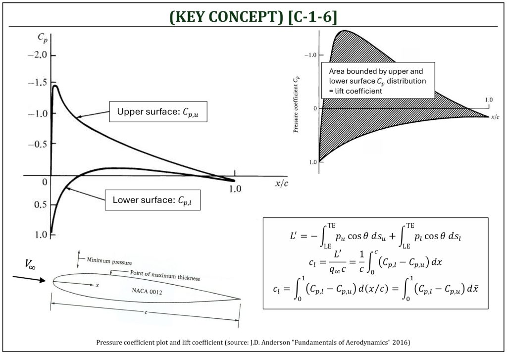
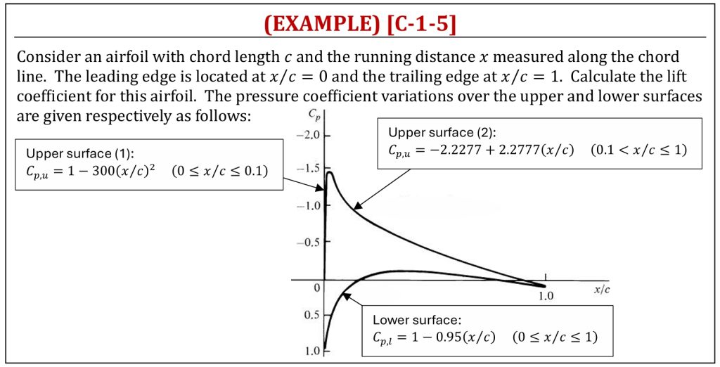
Close observation of Cp plot (i.e., NACA 0012 airfoil in a small angle of attack) indicates the following surface flow characteristics of the given airfoil.
- Upper surface: Cp at the leading edge starts from 1 (stagnation point). Cp starts to decrease (favorable pressure gradient) very rapidly (p < p∞) and reaches the minimum pressure point. After this minimum pressure point, Cp increases (adverse pressure gradient) toward the trailing edge.
- Lower surface: Cp at the leading edge starts from 1 (stagnation point). Cp starts to decrease (favorable pressure gradient) and then slightly increase (adverse pressure gradient) toward the trailing edge.
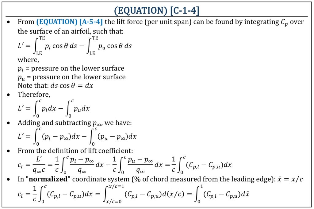
Lift Coefficient of an Airfoil
Pressure Coefficient
Lift Coefficient Calculation from Pressure Coefficient Distributions
References
- Introduction to Aerospace Flight Vehicles by J. G. Leishman (https://eaglepubs.erau.edu/introductiontoaerospaceflightvehicles)
- AirfoilTools (https://airfoiltools.com)
- Historynet (https://www.historynet.com)
- Fundamentals of Aerodynamics by J.D. Anderson, 5th ED, McGraw Hill, 2016
- Aerodynamics for Engineers by J. J. Bertin & M. L. Smith, 3rd ED, Cambridge University Press, 1997
- Aerodynamics for Engineering Students by E. L. Houghton & P. W. Carpenter, 4th ED, Edward Arnold, London, 1993
Media Attributions
If a citation and/or attribution to a media (images and/or videos) is not given, then it is originally created for this book by the author, and the media can be assumed to be under CC BY-NC 4.0 (Creative Commons Attribution-NonCommercial 4.0 International) license. Public domain materials have been included in these attributions whenever possible. Every reasonable effort has been made to ensure that the attributions are comprehensive, accurate, and up-to-date. The Copyright Disclaimer under Section 107 of the Copyright Act of 1976 states that allowance is made for purposes such as teaching, scholarship, and research. Fair use is a use permitted by copyright statute. For any request for corrections and/or updates, please contact the author.
