B-4: Ideal Flow Analysis (2)
Potential (Ideal) Flow Field Analysis (2 of 2)
Shigeo Hayashibara
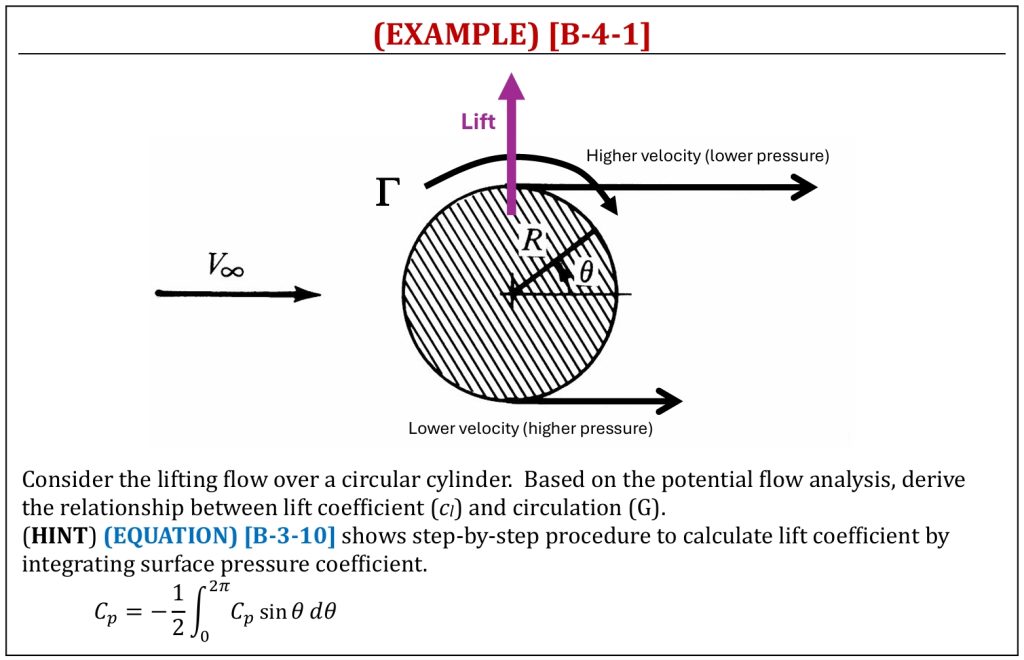
Lifting flow over a circular cylinder
Lifting Flow over a Circular Cylinder
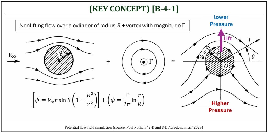
Recalling from B-4 (nonlifting flow over a circular cylinder), combining uniform flow + doublet will construct a simulated flow around a circular cylinder with no lift and no drag (d’Alembert’s paradox). This is called, “nonlifting” flow over a cylinder (as it generates no lift). Now, let us try simulating a “spinning” circular cylinder by adding the flow field circulation. This will construct a “lifting” flow over a circular cylinder. In order to do so, mathematically, let us add vortex flow with the strength Γ (this is the flow field circulation) onto the nonlifting flow over a cylinder of radius R.
Lifting Flow over a Circular Cylinder
Lifting flow: Stagnation Points
Lifting Flow over a Circular Cylinder: Stagnation Points
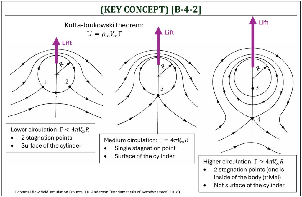
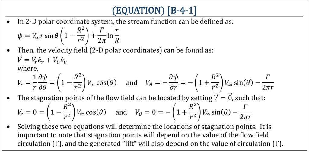
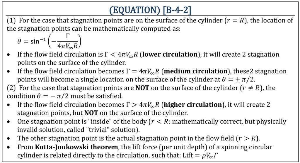
The stagnation points of the flow field (lifting flow over the circular cylinder) come with variety, depending on the amount of the flow field circulation (Γ). From the Kutta-Joukowski theorem, the lift (per unit depth) also depends on the amount of the flow field circulation (Γ).
Lifting Flow over a Circular Cylinder: Stagnation Points
Lift Calculation from Pressure Distributions
Real Flow over a spinning circular cylinder
The Magnus Effect
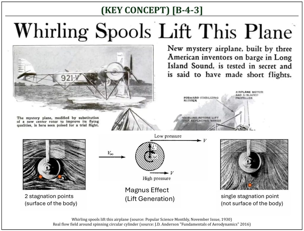
The nonsymmetric flows about the spinning bodies generate an aerodynamic force, which is perpendicular to the body’s angular velocity vector. This phenomenon is called the “magnus effect,” which is quite similar to the theoretical analysis of lifting flow over a circular cylinder. The relationship between the flow field circulation Γ (i.e., “rate of spin” of the real flow field) and the generated lift coefficient cl can be derived from the Kutta-Joukowski theorem.
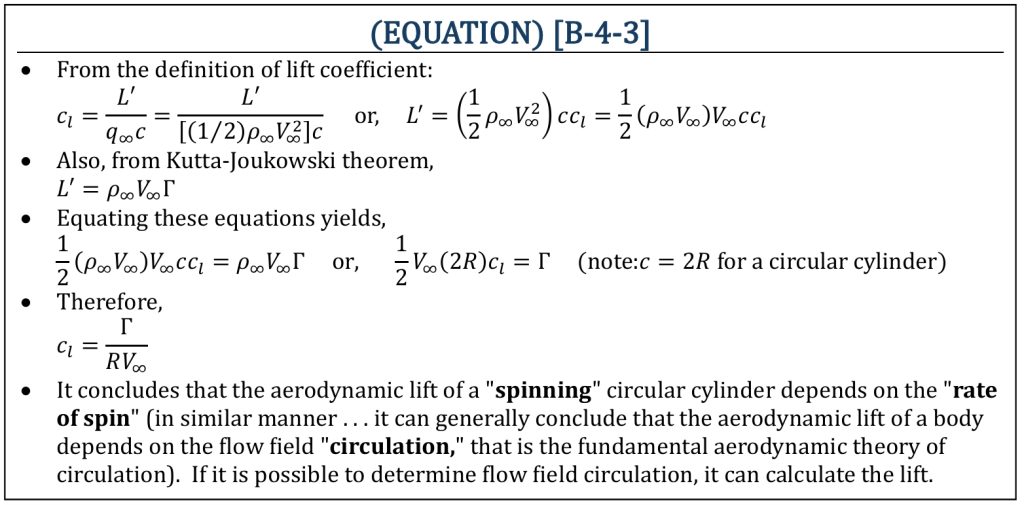
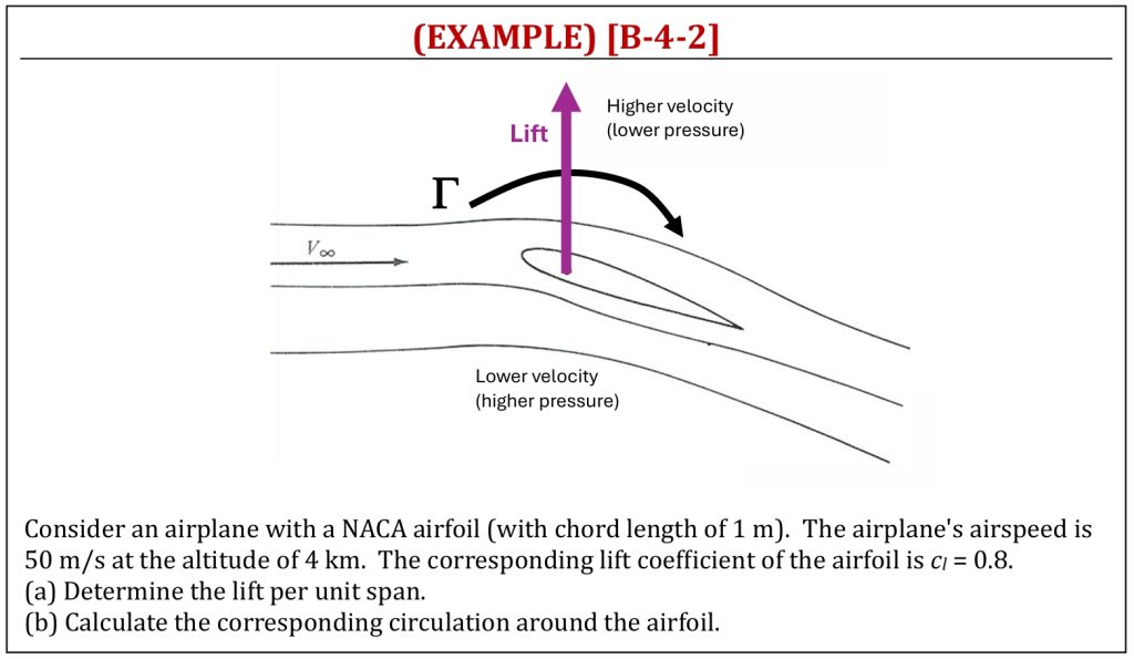
Circulation and Lift (Circulation Theory of Aerodynamics)
At this moment, let us review (KEY CONCEPT) [B-2-3] once again. Based on the potential flow analysis (pure mathematical analysis) of a lifting flow around a circular cylinder. Let us now replace the circular cylinder with an airfoil. This is the starting point of the potential flow analysis of a flow over an airfoil.
-
As we know from the analysis of a lifting flow around a circular cylinder, there are infinite numbers of valid theoretical solutions, corresponding to infinite choices of circulation. Basically, the location(s) of stagnation points depend only on the amount of circulation. Therefore, a potential flow field analysis over an airfoil, as we simplify many real flow field characteristics (especially viscosity), will result in non-realistic solutions of stagnation points . . .
-
However, a given airfoil at a given angle of attack should produce a single value (valid solution) of lift that should be more realistic against the given real flow field condition. We need an additional condition that fixes the amount of flow field circulation (the “correct” value) for a given airfoil at the given angle of attack . . .
-
If we apply potential flow field analysis (pure mathematical analysis) for a real flow field, an important additional condition will be crucial for a correct solution. This is called, “Kutta condition.” The Kutta condition will adjust the value of flow field circulation into a reasonable value (realistic for for real flow field), based on the fact that the flow at the trailing edge departs smoothly in a real flow field.
Starting Vortex
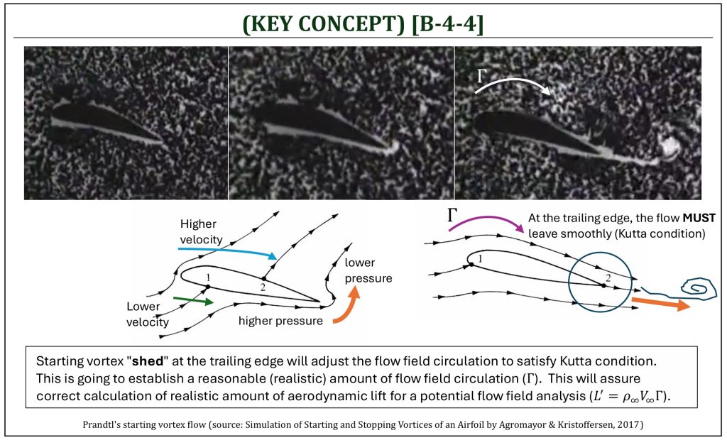
Let us learn from the nature of the real flow field. Experimental observation for the development of the flow field around an airfoil, which is set into motion from an initial state of rest, provides interesting insight into the nature of real flow around an airfoil. What happens when the flow field is established around an airfoil . . . this is a classical “starting vortex” formulation due to an “impulse start” of the real flow field.
-
The flow tries to curl around the sharp trailing edge from the bottom surface to the top surface. This is because the trailing edge is the point where higher pressure (bottom surface) meets the lower pressure (upper surface). A temporary stagnation point will be formed on the upper surface.
-
The upper surface stagnation point starts moving toward the trailing edge.
-
The flow is smoothly leaving the top and bottom surfaces of the airfoil at the trailing edge and the flow field achieves the steady-state condition.
The starting vortex is the “nature’s own way” to adjust the realistic flow field around an airfoil. By shedding an appropriate amount of starting vortex, the proper amount of flow field “circulation” is established, so that the the flow at the trailing edge can leave smoothly. This is called, the Kutta condition. In a potential flow field analysis, it is so important to mathematically incorporate the Kutta condition to assure realistic (i.e., correct) flow field solutions. This is going to be more clearly illustrated in B-5 (Joukowski Airfoils and Flow Mapping).
- For a trailing edge with finite angle: V1 = V2 = 0 (thus, a stagnation point is formed at the trailing edge).
- For a “cusped” trailing edge (continuous smooth curved surface on both upper and lower surface, so the trailing edge angle cannot be well defined; this is very common for an airfoil design): V1 = V2 ≠ 0 (thus, the flow departs smoothly at the trailing edge).
Circulation and Lift
References
- Popular Science Magazine (https://www.popsci.com)
- Simulation of Starting and Stopping Vortices of an Airfoil by Agromayor & Kristoffersen, 2017
- Fundamentals of Aerodynamics by J.D. Anderson, 5th ED, McGraw Hill, 2016
- Aerodynamics for Engineers by J. J. Bertin & M. L. Smith, 3rd ED, Cambridge University Press, 1997
- Aerodynamics for Engineering Students by E. L. Houghton & P. W. Carpenter, 4th ED, Edward Arnold, London, 1993
Media Attributions
If a citation and/or attribution to a media (images and/or videos) is not given, then it is originally created for this book by the author, and the media can be assumed to be under CC BY-NC 4.0 (Creative Commons Attribution-NonCommercial 4.0 International) license. Public domain materials have been included in these attributions whenever possible. Every reasonable effort has been made to ensure that the attributions are comprehensive, accurate, and up-to-date. The Copyright Disclaimer under Section 107 of the Copyright Act of 1976 states that allowance is made for purposes such as teaching, scholarship, and research. Fair use is a use permitted by copyright statute. For any request for corrections and/or updates, please contact the author.
