1. Introduction

1.1 Review of descriptive statistics

When working with a data set, we use the notation x_i for the i^th data point in a data set. For example, if we were working with the following data set of airplane’s speeds

we would call x₁ = 500 and x₂ = 700 etc. Of course, in the “real world” it is common to work with extremely large data sets so it becomes necessary to calculate the descriptive statistics, which allow us to understand the various things a data set is telling us. These descriptive statistics are, generally speaking, divided into two categories: measures of central tendency or measures of dispersion. The first category, measures of central tendency, attempts to simply describe the average value or middle of the data set; namely, a few examples of the measures of central tendency are the median and the mean as given in definitions (Definition) 1.1.1 & 1.1.2. The second category, measures of dispersion, attempts to describe how spread out the data set is; namely, a few examples of the measures of dispersion are the range and the variance as given in Defintion 1.1.3 & 1.1.4.

It is common that many resources will attempt to describe a data set by graphical illustration. Although these illustrations are useful, it is essential to remember that as scientists we cannot rely on graphical analyses to draw conclusions. Rather, we require formal analytical mathematical statements. For example we know that for a data set to be considered a normal distribution the data set must have most of the data frequency near the middle with a symmetrical pattern and the frequency should be less the further away from the middle. Hence, if a histogram is constructed it should look like this:

 

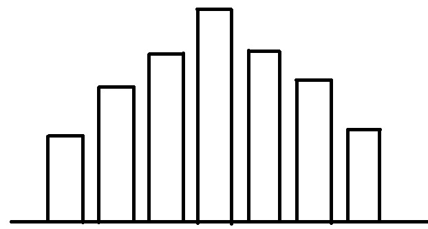
It is essential to understand that this graph alone does not prove nor reject the hypothesis that this distribution is normal. If one wanted to attempt to validate the hypothesis that this distribution is normal, then a formal “test of normality,” including a formal computed analytical value to be compared to a formal analytical critical value, would be required. Prior to getting ahead of ourselves, let us summarize a few common descriptive statistics with proper analytical formulas.

 

Example 1.1.1

Find the mean of data set 1.1.1

[latex]\bar X = \frac{1}{3}\left( {500 + 700 + 900} \right) = 700[/latex]

Example 1.1.2

Find the mean of data set 1.1.2

[latex]\bar X = \frac{1}{3}\left( {20 + 30 + 40} \right) = 30[/latex]

 

Example 1.1.3

Find the median of data set 1.1.1

Firstly, we must rank the data set, which in this case is already ordered, as

X₁= 500 & X₂ = 700 & X₃ = 900.

Then, the median is simply found as the middle value. In this case
[latex]\tilde X=700[/latex]

It is important to note that the measures of central tendency alone do not completely describe the data set under consideration. For example, if we compute the mean & median of both data sets 1.1.3A & 1.1.3B, then we will find the results to be the same as 50. However, it is obvious that the data sets are quite different; namely, the first data set is very clustered together while the second data set is much more spread out.

Thus, we will need to consider measures of dispersion in addition to finding the mean or median. Now, a small value of dispersion would imply that the data set is closely clustered together while a large value of dispersion would mean the data set is more spread out; hence we would expect data set 1.1.3A to have smaller measures of dispersion than data set 1.1.3B. This is indeed true as we will find the variance of 1.1.3A is 17, while the variance of 1.1.3B is 312.50.

 

Example 1.1.4

Find the range of data set 1.1.1.

Firstly, we must rank the data set, which in this case is already ordered, as X₁= 500 & X₂ = 700 & X₃ = 900.

Then, the range is simply the largest value minus the smallest value X₃ – X₁ = 900 – 500 = 400.

 

Example 1.1.5

Find the variance of data set 1.1.3A.

First, we must find the mean, which in this case is 50. Next, it helps to use the following table to simplify the procedure for computing our formula.

If we sum the last column we will find the sum of the squares, [latex]\sum {\left( {\;{x_i} - \bar X} \right)^2}[/latex]

which in this example is 68. The variance is then found as this value divided by n-1. In this example we would divide by 4 to find the variance to be 68/4 = 17.

 

The standard deviation is essentially measuring the same thing as the variance did, however, by taking the square root we are bringing the measure back to the same dimension / units of the original data. For example, if we computed the variance of data set 2 we would find it to be 100. However, this would actually be in units of mph² which may not be the most practical in applications, yet the standard deviation would be in units of just mph.

Example 1.1.6

Find the standard deviation of data set 1.1.2.

First, we must find the variance which as noted above is 100 mph². Thus, by definition, the standard deviation is the square root of variance = [latex]\sqrt {100mp{h^2}} = 10mph.[/latex]

It is also very important to keep in mind “unit bias” when performing data analysis. For example if we were to compare our prior data set of car speeds

to our prior data set of plane speeds

it should be apparent that a 200 mph difference of speed in one context is quite different than a 200 mph difference of speed in another (have you ever been passed by another vehicle on the freeway going 200 mph faster?). This “unit bias” can be eliminated by transforming the raw data to the “Z scores” which, as the next definition will outline, is done simply by dividing the individual data point’s deviation by the standard deviation. In fact, this standardization will show that the third car, which is going 10 mph above the mean of that data set, has the same “Z score” as the third plane, which is going 200 mph above the mean of that data set. Hence, one can infer that a 10mph deviation in car’s speed is essentially equivalent to a 200 mph deviation in an airplane’s speed.

 

Example 1.1.7

Compute the Z score for all data points in data sets 1.1.1 & 1.1.2.

 

1.2 Introduction to correlation & regression

To conclude this introductory chapter, in this section we will briefly introduce the idea of correlation between two data sets x and y which we will assume both contain an equal number of elements, namely n elements in each data set. The main idea with correlation, or perhaps the main question to ask, is this: is there a pattern between the two data sets? A common mistake that can be made is thinking that the only way to have a correlation between data set x and data set y is that the pattern between x and y must be linear, perhaps y = 2x or y =3x etc. However, this is not correct as there are many other correlation patterns which can occur between two data sets such as quadratic fits or exponential fits. Later on in the textbook we will study the concept of building a predictive model from an x,y data set pair known as a linear regression model, and this tool is one of the most widely applicable statistical models. Of course the linear regression model is a primary purpose of our study and for students of engineering or the sciences this linear predictive data model can be extremely useful. But, it is important to note that linear fits are not the only fit and just because data is correlated does not mean that a linear regression model will work. In mathematical terms one might say that a solid value of correlation is a necessary condition for a linear regression model to work, but it is not a sufficient condition!

The correlation between two data sets is defined in terms of the deviation between the Z scores of the x data set and the Z scores of the y data set. No deviation between the data set’s Z scores is defined as perfect correlation, while an extreme amount of deviation between the data set’s Z scores is defined as a low correlation or near zero correlation. For example, if we were to revisit example 1.1.5 and call the data set of car’s speeds the x data set and the data set of airplane’s speeds the y data set and then compute the differences of those Z scores, we would essentially be studying the correlation pattern between the cars and airplanes. It is worthy to note, prior to working out the details of this example, that in this case we expect a perfect correlation as we have previously discovered that the car’s speeds and airplane’s speeds go up in a uniform pattern of 1 standard deviation each data point.

Example 1.2.1

Compute the difference between the Z score for data points sets 1.1.1 & 1.1.2.

To begin we recall from Ex 1.1.7 the Z score which we previously computed and then label accordingly as done above. To complete this example we then simply compute the differences

We observed, as expected, that the total differences are zero which shows a perfect correlation between our data sets.

Now, for a formal definition of correlation we use the following definition which has the interpretation similar to a percent: r near 1 is near perfect correlation (analogous to 100% being near perfect chance) while r near 0 is low correlation (analogous to 0% being near no chance).

 

Example 1.2.2

Compute the correlation for data pairs from data sets 1.1.1 & 1.1.2.

To begin, we recall from Ex 2.1.1 the differences in the Z score which we previously computed and then we must compute the squared differences

Now, to complete the problem we utilize the definition

[latex]r = 1 - \frac{1}{{2\left( {n - 1} \right)}}\mathop \sum \limits_{i = 1}^n {\left( {{Z_{xi}} - {Z_{yi}}} \right)^2}[/latex]

with n= 3. Doing so this yields the solution

[latex]r = 1 - \frac{1}{{2\left( {3 - 1} \right)}}\left( {{0^2} + {0^2} + {0^2}} \right) = 1 - 0 = 1[/latex]

We observed, as expected, that the correlation here is a perfect correlation = 1, which again we can informally view analogously to a percent so in an informal sense we can think this data set is 100% correlated.

Example 1.2.3

Compute the correlation for data pairs from the data set 1.2.1 below.

Where it is given that the mean of x is 3 and y is 6, while the standard deviation of x is 1.58 and of y is 3.39.

To begin, we must compute the Z scores in for x and y separately

Now, the differences in the Z scores must be computed and then their squares

Finally, to complete the problem we utilize the definition

[latex]r = 1 - \frac{1}{{2\left( {n - 1} \right)}}\mathop \sum \limits_{i = 1}^n {\left( {{Z_{xi}} - {Z_{yi}}} \right)^2}[/latex]

with n= 5. Doing so yields the solution

[latex]r = 1 - \frac{1}{{2\left( {5 - 1} \right)}}\left( {0.007376 + 0.001844 + \ldots } \right) = 1 - 0.02 = 0.98[/latex]

We observed, as expected, that the correlation here is a very high correlation = 0.98 as expected because in the data set we can observe the pattern Y being approximately 2x. Again we can informally view analogously to a percent so in an informal sense we can think this data set is 90% correlated.

It is worthy to note that while the prior definition is the theoretically correct and the original definition it is not always the commonly used one. By putting in the definitions of Z scores and performing some algebraic manipulation the following alternate definition for correlation can be obtained and is useful since it is all in terms of values from the data set, hence it is not needed to first compute the Z scores. Also, for mathematical interest the correlation can be written as the covariance of X and Y divided by the products of their standard deviations. Namely, we can write

[latex]r = \frac{{cov\left( {x,y} \right)}}{{{s_x}{s_y}}}[/latex]

 

The above definition will yield the exact same value as the correlation definition provided in the prior definition 1.2.1, and is actually derived from that prior definition, but this new formula is often preferred when coding formulas as it can be computed directly from raw data as opposed to needing the normalized “z values.”

One of the most useful applications of correlation for an (x,y) pair data set is to build a predictive model to predict the y variable in terms of the x variable as input. Namely, it is desired to create an equation of the form

[latex]\hat y = mx + b,[/latex]

where the hat notation is utilized to distinguish it as being a predicted value; perhaps a future or forward data point.

 

Example 1.2.4

Compute the linear regression line for data pairs from the data set 1.2.1.

To begin, we recall from the prior solution that

[latex]{s_y} = 1.52,{s_x} = 0.71,\bar y = 6,\bar x = 3\;and\;r = 0.9[/latex]

Hence, we can compute

[latex]m = r\left( {\frac{{{s_y}}}{{{s_z}}}} \right) = 0.9\left( {\frac{{1.52}}{{0.71}}} \right) = 1.93[/latex]

and

[latex]\beta = \bar y - m\bar x = 6 - 1.93*3 = 0.21[/latex]

Which yields our solution as the predictive model of our linear regression line

[latex]\hat y = 1.93x + 0.21.[/latex]

The linear regression line has far reaching applications in various fields such as engineering or science and finance applications. For example, our data ended at the value of x being 5 so one could use the linear regression line to expand beyond that, perhaps to find the predicted y value associated with a future x of 6 as

[latex]\hat y\left( 6 \right) = 1.93\left( 6 \right) + 0.21 = 11.79.[/latex]

For another example, our data set contained only integer values of x being 1 then x being 2 etc., and one could use the linear regression line to fill in between that, perhaps to find the predicted y value associated for a half way value x of 1.5 as

[latex]\hat y\left( {1.5} \right) = 1.93\left( {1.5} \right) + 0.21 = 3.11.[/latex]

There are many other applications, and of course restrictions to, the linear regression line and this will be a central theme of the later chapters of this textbook. However, prior to continuing with our development it is necessary to overview, or perhaps receive for the informed reader, some key principles from the mathematical theory of probability which are contained in Chapter 2. Due to the fact that this text is designed as a self-contained resource, these principals in Chapter 2 are developed “from the ground up” and the informed reader may be able to jump forward at this point. Any reader who has the knowledge equivalent to a Junior or Senior year university level course in mathematical statistics and/or introductory probability theory can most likely jump to Chapter 3. Regardless of that progression, it is important to close this Chapter with one essential principal regarding regression: while it is logical that it only makes sense to use a linear regression model for a data set which is highly correlated, that does not ensure that the linear regression model will work or be statistically valid. Namely, it is vital to understand, as previously stated, that from a mathematical point of view one can say that a solid value of correlation is a necessary condition for a linear regression model to work, but it is not a sufficient condition!

1.3 A brief comment about multivariable data

While the purpose of this textbook is for engineering students to obtain the knowledge needed to understand the underlying mathematical theory of probability, as opposed to an introduction to the many methods of inferential statistics & data analysis, it is worthy to include here a quick discussion about how to deal with data sets of more than two variables. Namely, one of the most common questions that arises is: “now that we have the definition of correlation between x & y, how do we generalize that to a data set that has more than two variables, for example x & y & z?” And, the answer to this question is that generally we do not have a “multi correlation,” but in the following example a method is outlined as to how such a measure can be computed.

The data set below was used in a research study to predict the value of an exchange traded fund called DJD, which is a very popular investment instrument that is designed to track the famous United States DOW JONES index; however, this index only includes a subset of the index of companies that have either maintained or raised their dividends over the last year, hence it is often preferred by investors looking for a somewhat conservative and safe investment. Now, the goal of the research study was to determine a statistical model that utilized macroeconomic predictor variables to make a mathematical prediction of the fair value of DJD. A data set of monthly values from 2016 to 2109 was obtained, and a subset of that data is listed below for illustration where the predictor variables have been normalized. For those interested in the details the values used here were: Consumer Price Index ( AKA “CPI” or the government’s measure of consumer inflation ), Producer Price Index ( AKA “PPI” or the government’s measure of product cost inflation ), Gross Domestic Product ( AKA “GDP” ), and the Federal Funds Rate ( AKA “FFR” ), with all data being publicly available freely from official government websites.

Now, in the analysis one of the worst things that can be done when creating such models is to have high amounts of inter correlation within the predictor variables; this applies regardless if the model being used is regular regression like was done in this research or more advanced modern models such as machine learning methods (of course technically regression is the nicest example of supervised machine learning). Often a first investigative step is to run a correlation matrix, which will yield results that look something like

The issue with this procedure is that it is not really a multi variable correlation, rather it is a list of multiple individual correlations. For example, the value 0.984656 is the correlation between CPI & PPI in isolation, while the value of 0.968366 is the correlation between PPI & GDP in isolation etc.

The correlation matrix does provide information, but it does not really answer the question of how multi correlated these variables are. For example, the largest correlation between any two variables is seen between FFR and GDP, as that pair has the largest value of correlation being 0.986. However, when this was computed the computation was done in isolated. Namely, when calculating this the same correlation formula from our prior section

[latex]r = 1 - \frac{1}{{2\left( {n - 1} \right)}}\mathop \sum \limits_{i = 1}^n {\left( {{Z_{xi}} - {Z_{yi}}} \right)^2}[/latex]

was used with the x variable being FFR and the y variable being GDP, but none of the other variables were considered in the computation ( i.e. it was done in isolation ). Thus, this measure does not really define how one of the variables, say GDP, is correlated to all of the other variables. One informal resolution to this problem is to add up all of the individual correlations, e.g. 0.986 + 0.968366 + 0.983551. Doing so we would obtain the total for GDP to be 2.937917. Then similarly the total for CPI to be 2.933651, the total for PPI to be 2.895676 and the total for FFR to be 2.894098. While this does provide the information that GDP does appear to have the worst inter correlation, with CPI not so far behind, this is not exactly a mathematically proper definition.

In order to measure how correlated one variable is related to multiple other predictor variables the following procedure is often applied. Firstly, take the variable of concern and move it into the column of the response variable; for example if we were to do this for GDP our data set would now look like

or if we were to do this for CPI our data set would now look like

Now, the next step is to run a multivariable regression model with the remaining predictors being used as normal, but the Y variable not being the original data desired but instead replaced by the predictor variable under consideration. Then after running this multivariable regression model from the output the value of the so called coefficient of determination ( AKA R squared ) should be noted. For example doing so for data set 1.32, which has GDP as the response, above yields R² = 0.987513087343, so this is essentially a measurement of how GDP is totally correlated ( technically predicted by ) the predictor variables CPI, PPI and FFR. Likewise, doing so for data set 1.33, which has CPI as the response, above yields R² = 0.984192914938173, so this is essentially a measurement of how GDP is totally correlated (again, technically predicted by) the predictor variables PPI, GDP and FFR.

 

Example 1.3.1

Compute the VIF for both GDP and CPI from data set 1.3.1, and using the previously obtained information.

To solve this it is needed to obtained the coefficients of determination, but those have already been provided. Thus, we can quickly compute

[latex]VIF\left( {GDP} \right) = \frac{1}{{1 - {\rm{\;}}0.987513087343}} = 80.08[/latex]

and

[latex]VIF\left( {CPI} \right) = \frac{1}{{1 - 0.984192914938173}} = 63.26[/latex]

Now, while these computations are very interesting and provide information, the big question is do they really answer the question as to how “multi correlated” one variable is to all of the others, and the answer is sort of! The coefficient of determination does tell us what percentage of the variance in the variable under consideration is explained by a regression model created from the other variables, and while this is not exactly a correlation it does provide similar information. However, it is important to remember the main question in applications is not really to see how correlated one variable is to the others, but will putting both of them into the model cause an issue? The general rule of thumb is if a variable has a VIF > 10 then it would be advised to proceed with caution as to using the variable, and if a variable has a VIF closer to 100 then it absolutely should not be included. Moreover, what is interesting to observe is how the variance inflation factor sniffs out minor details. Namely, in this example we found, using the not so formal method of adding up all the individual correlations, that CPI and GDP were about the same, 2.933651 and 2.937917 respectively. However, the VIF method is much more accurate as it shows that GDP had a much higher value, 80 compared to 60, thus it provides a clear solution that of these variables GDP is the most correlated, formally what is referred to as multicolinearity.

It is important for the reader of this text, who again should be more focused on understanding the mathematical theory of probability, that the big take away is that while we do not really have a definition of multi correlation, this method of VIF is an important tool which can be used to narrow down a data set; hence, avoiding redundancy within the data set which can be an issue if one predictor variable is extremely correlated to many of the other predictor variables. Lastly, to close this chapter the formal definition of the coefficient of determination is provided for mathematical completeness, but no examples as those are generally discussed in courses such as inferential statistics or regression analysis.