4. Introduction Continuous Probability Theory

4.1 continuous random variables

In the following section we will define one of the most important topics in the mathematical theory of probability, the continuous probability density function. It is from this density function that many results such as probability solutions and expected values will be derived. However, prior to doing so, it is important to note that for simplification through the remainder of this text, which is designed to for a first course in probability theory, we will only be considering examples of independent continuous random variables, hence all computations will involve single variable functions and their corresponding calculus computations

At this level we will not attempt to develop the derivation or underlying motivation for our probability density functions; rather, we will define a density function f(x) for a random variable X to be the function that creates the probability as

[latex]P\left(A < x\le B\right)=\int_{A}^{B}{f\left(x\right)dx.}[/latex]

Now, this probability density function must meet two basic properties, which are in line with the axioms of probability:

NOTE: if you have an example of a function desired to be used for a density that meets criteria (i) but not (ii) then you can create a valid density by the normalization process (similar to that of normalizing a vector) by dividing the constant [latex]K=\int_{-\infty}^{+\infty}f\left(x\right)dx[/latex], as one will find the function

[latex]\frac{1}{K}f\left(x\right)[/latex]

will be a valid density function.

Example 4.1.1

Find the normalized density for a density of the form

defined for x > 0 and zero elsewhere.

To begin we note that we must satisfy properties (i) and (ii) of definition 4.12. Now, it is first observed that property (i) is met because the exponential function is a strictly positive function. However, property (ii) is not met because

Thus, using the logic from above we take the constant

to create the normalized density to be the so called exponential density

Example 4.1.2

Find the value of C so that the function, which is defined as

or 0 otherwise, will be a valid density.

To begin we note that we must satisfy properties (i) and (ii) of definition 4.12. Now, it is first observed that property (i) is met because this parabolic function will be above the x axis, with zeros at x=1 and x=0, provided that the value of C is positive. Now, property (ii) is not met until we specify the value of C, thus we compute

[latex]\int_{-\infty}^{+\infty}{f\left(x\right)dx=\int_{-\infty}^{0}{0dX\ +\int_{0}^{1}{C\bullet X\bullet\left(1-X\right)dX+\int_{1}^{\infty}{0\ dX=C\left(\frac{1}{2}-\frac{1}{3}\right)=\frac{C}{6}.}}}}[/latex]

Now, in order to make this a valid density we must choose C=6.

Example 4.1.3

Verify that the uniform density

or 0 otherwise, is a valid probability density function.

To begin we note that we must satisfy properties (i) and (ii) of definition 4.12. Now, it is observed that property (i) is met because the function is a constant positive value. In verifying property (ii), we obtain

[latex]\int_{-\infty}^{\infty}{f\left(x\right)dx=\int_{\infty}^{L}0dx+\int_{L}^{R}{\frac{1}{R-L}dx}+}\int_{R}^{\infty}{0dx=\frac{R-L}{R-L}}=1.[/latex]

Example 4.1.4

Verify that the standard normal density

[latex]f\left(x\right)=\frac{1}{\sqrt{2\pi}}e^\frac{-x^2}{2}[/latex]

is a valid probability density function.

To begin we note that we must satisfy properties (i) and (ii) of definition 4.12. Now, it is first observed that property (i) is met as the exponential function is a strictly positive function. However, we must verify property (ii), and in doing so we obtain

[latex]\int_{-\infty}^{\infty}{f\left(x\right)dx=\int_{-\infty}^{\infty}{\frac{1}{\sqrt{2\pi}}e^{-0.5x^2}dx}}[/latex]

This is a very difficult integral to do in closed form, but one can compute numerically and verify that this integral is indeed equal to 1, hence the provided density is a valid probability density function!

4.2 commonly utilized continuous density functions

It is worthy to take note of a few of these common density functions as they will frequently be used in examples as we move forward and have many common real world applications! The following are the most likely examples that you will encounter are:

The exponential density is

which is defined for x > 0,

and the uniform density is

which is defined for L < x < R,

where both of these densities serve useful for textbook illustrative examples due to the fact that the resulting integrals turn out to be doable without the need for complicated integration techniques.

The normal density is

which is defined for all x, and this density is by far one of the most applicable in real world modeling applications.

The standard normal density is

which is defined for all x, and is a special case of the normal density with mean µ=0 along with variance 𝞼=1, serves as the backbone of many theoretical mathematical statistical results such as the famous central limit theorem.

The T density is

[latex]f\left(x\right)=\frac{\mathrm{\Gamma}\left(\frac{v+1}{2}\right)}{\sqrt{v\pi}\mathrm{\Gamma}\left(\frac{v}{2}\right)}\left(1+\frac{x^2}{v}\right)^{-\frac{v+1}{2}}[/latex]

which is defined for x > 0 with v being the degrees of freedom. This density is utilized in applications as an approximation for the normal density when some of the information of the population mean, µ, or variance, 𝞼² , is unknown.

The chi squared density is

which is defined for x > 0, with v being the degrees of freedom. This density is utilized in applications for error analysis when considering the sum of squares error and/or Goodness of fit error analysis.

The F density is

which is defined for x > 0, where d₁ and d₂ are the degrees of freedom, numerator and denominator respectively. This density is related to a ratio of two chi squared densities and is very useful in a great deal of applications. especially the analysis of linear regression.

The logistic density is

which is defined for x > 0, with s representing the scale not standard deviation as one might expect. This density is very useful in the analysis of regression when applied to case when the response variable in the form of a categorical “1/0” variable (AKA logistic regression).

Some more generalized “abstract” examples are:

The Beta density is

which is defined for x > 0.

The factor 𝛤 is the so called “Gamma function,” which normalizes the density. There is

a formal definition of this function valid for any values of n, but for our

purposes it will suffice to use the definition:

[latex]\mathrm{\Gamma}\left(n\right)=\left(n-1\right)![/latex]

for integer values

[latex]\Gamma \left( \frac{n}{2}\right)=\sqrt \pi \frac{(n-2)!!}{2^\frac{n-1}{2}}[/latex]

for halves using odd n; note

Now, we have several probability density functions let us look at some examples

Example 4.1.5

For the exponential density

[latex]f\left(x\right)=e^{-x}[/latex]

Find the probability P(0<x<5).

To begin we know the density is as given above so we just need the probably integral

Thus, we compute

[latex]\int_{0}^{5}{e^{-x}dx=\left[-e^{-x}\right]_{x=0}^{x=5}=1-e^{-5}\approx0.993}[/latex]

Hence, we have computed the probability P (0<x<5) = 99.3%.

Example 4.1.6

For the uniform density

with R = 10 and L = 0 find the probability P (0<x<2).

To begin we note that our density will be

and the probability integral will be

Thus, we compute

[latex]\int_{0}^{2}{\frac{1}{10}dx=\left[\frac{x}{10}\right]_{x=0}^{x=2}=0.2}[/latex]

Hence, we have computed the probability P(0<x<2) = 20%.

Example 4.1.7

For the standard normal density

[latex]f\left(x\right)=\frac{1}{\sqrt{2\pi}}e^\frac{-x^2}{2}[/latex]

find the probability P(0<x<2).

To begin we know the density is as given above so we just need the probably integral

Thus, we compute

[latex]\int_{0}^{2}{\frac{1}{\sqrt{2\pi}}e^\frac{-x^2}{2}dx.}[/latex]

However, this integral, which is ultimately an integral of the form , is not solvable in closed form so numerical approximations will be required (which yield the solution of approximately 47%) . In the next chapter we will further discuss how to work with normal density, as it is one of the most important densities if not the most important, and we will look at some applications of nice function in MATLAB. For now, we will move on with developing further properties of probability distribution theory, namely the expected value and variance.

In the following section we will define two extremely useful properties of statistics the expectation and the variance. Generally speaking one can view these in an analogous manner as the expected value and variance are interpreted in elementary data analysis. Namely, the expectation ( AKA expected value ) can be viewed as the average value or “what we expect to get on average,” which is frequently just called the mean and often the symbol µ is utilized. And, the variance can be viewed as a measure of dispersion or “how spread out is the data,” which is often notated by the symbol 𝞼². For simplification we will define, for a random variable x, the expectation as E(x) and moving forward write all expressions, definitions and so forth in terms of E(x) as not only is it good practice for consistency, but it is also the proper and formal way to define things!

4.3 expectation and variance

At this time we will focus on solving examples and address interpretations along with theoretical implications for later studies. However, it is good for the reader to understand the solution obtained is an expected value and not a probability, i.e. it does not have to be within the usual range of 0 to 1 rather the answer can be viewed as just a number!

Example 4.3.1

Find the expectation for the Standard Normal density

[latex]f\left(x\right)=\frac{1}{\sqrt{2\pi}}e^{-0.5x^2}[/latex]

To begin we recall the above definition of the expectation is .

and we compute

[latex]E\left(x\right)=\int_{-\infty}^{\infty}{x\bullet\frac{1}{\sqrt{2\pi}}e^{-0.5x^2}dx=\left[-\frac{1}{\sqrt{2\pi}}e^{-0.5x^2}\right]_{-\infty}^\infty=0.}[/latex]

Example 4.3.2

Find the expectation for the particular case of the Beta density

To begin we recall the above definition of the expectation is

[latex]E\left(x\right)=\int_{\mathrm{\Omega}}{x\bullet f\left(x\right)dx}[/latex]

and we compute

[latex]E\left(x\right)=\int_{0}^{1}{X\bullet\left(6X\bullet\left(1-X\right)\right)dX=\frac{1}{2}.}[/latex]

where the symbol µ is representing the value of the expectation for the density, as often the expectation is interpreted as a mean or average value. Again, at this time we will quickly observe solving an example and leave interpretations along with theoretical implications for later studies.

Example 4.3.3

Find the variance for the Standard Normal density

[latex]f\left(x\right)=\frac{1}{\sqrt{2\pi}}e^{-0.5x^2}[/latex]

To begin we recall the above definition of the variance is

[latex]VAR\left(x\right)=\int_{\mathrm{\Omega}}{\left(x-\mu\right)^2\bullet f\left(x\right)dx}[/latex]

Thus, we compute

[latex]VAR\left(x\right)=\int_{-\infty}^{\infty}{\left(x-0\right)^2\frac{1}{\sqrt{2\pi}}e^{-0.5x^2}dx=1.}[/latex]

For the purpose of this textbook study, the preceding definitions will suffice

to cover all forthcoming needed mathematical theory. However, we will close this

section with the following definitions and results as they can be very useful in

applications to actually compute the expectation and/or variance for a density without

conducting the integrals from the prior definitions.

4.4 normal density and its small sample approximation

To begin our illustration we will actually steal the results from a couple of example forthcoming in the next chapter ( examples 5.12 & 5.1.3 ), and while we will not yet go into the details of the calculation, for the result called a P value, it is interesting to note that the solution yielded the results of 0.0062 if the normal density was utilized or 0.0027 is the T density was used with v=5 degrees of freedom. Moreover, if we increase the degrees of freedom, say to 50 then 100, we obtain the results of this P value to be 0.008 then 0.007 respectively. Thus, one can conclude that as the degrees of freedom for the T distribution get larger the result gets closer to the normal distribution! Of course the question here often comes as to what exactly are degrees of freedom? The exact answer to this question depends on the exact application and/or statistical experiment under consideration, but in most cases one can think that the degrees of freedom are about the same as, or very closely related to, the sample size of the data set being used in the statistical study. For example, in the classical hypothesis testing, which is one of the most commonly applied techniques, if the T density is used as the density the degrees of will actually be one less than the sample size of the data set, e.g. v= n-1. Thus, it is often comment to think of the T density as a small sample size approximation of the normal density. Moreover, one can actually prove that

[latex]\lim_{n\to\infty}{\left(\frac{\mathrm{\Gamma}\left(\frac{v+1}{2}\right)}{\sqrt{v\pi}\mathrm{\Gamma}\left(\frac{v}{2}\right)}\left(1+\frac{x^2}{v}\right)^{-\frac{v+1}{2}}\right)}=\frac{1}{\sqrt{2\pi}}e^{-0.5x^2}[/latex]

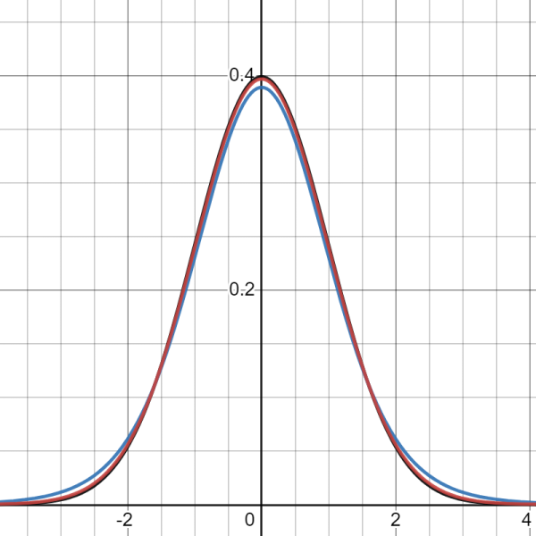
This result can be viewed visually below in the graphs, where the BLUE is the T density with 5 degrees of freedom, and the RED is the T density with 50 while the OTHER is the normal distribution.

It is worthy to note that in most applications it is not practical to actually find the population mean nor variance, hence the values needed for the true normal density; thus, in practice most applications will use the T density as the model. The T density actually provides results that are a little more conservative, which is always a good thing to do when doing statistical analysis!

4.5 examples with application to error analysis

To begin our first application we will assume an experiment has been done – either building a statistical model such as regression or a regular experiment such as trying a new method to make a part for an airplane – and it is desired to conduct analysis on the mean squared error, e.g. on the term

where the regular y represents the data and the [latex]\hat{y}[/latex]  is used for either the approximated value from the model or the desired value obtained from the underlying engineering scientific theory. Moreover, if one can assume that each of the

terms are normally distributed, and each

is independent of all of the others, then the sum of their squares would be a chi-squared distribution

[latex]f\left(x\right)=\frac{1}{2^\frac{k}{2}\mathrm{\Gamma}\left(\frac{k}{2}\right)}x^{\left(\frac{k}{2}\right)-1}e^{-\frac{x}{2}}[/latex]

where in this example the notation k, which is referred to as degrees of freedom, is how many independent variables are added. Hence, one can conclude that the distribution

[latex]f\left(x\right)=\frac{1}{2^\frac{v}{2}\mathrm{\Gamma}\left(\frac{v}{2}\right)}x^{\left(\frac{k}{2}\right)-1}e^{-\frac{x}{2}}[/latex]

can be used when analyzing the term

[latex]\sum_{i=1}^{k}{\left(y_i-\hat{y}\right)^2.}[/latex]

In many applications it is desired to evaluate the Mean Squared Error “MSE,” which is defined as

[latex]MSE=\frac{1}{k}[/latex]

[latex]\sum_{i=1}^{k}\left(y_i-\hat{y}\right)^2[/latex]

However, it is commonly not possible to compute this value on the whole data set; often it is not possible to obtain the full data set, so only a small data set is obtainable & analyzed, or only a subset is used for the computation initially as the other part of the data set is used to create the model ( AKA training/testing data ). If the full data set is of size n, and the total held back for testing is of size k, the MSE to compute would be

[latex]MSE=\frac{1}{k}\sum_{i=k+1}^{k+n}\left(y_i-\hat{y}\right)^2[/latex]

A method known as statistical learning, which can be defined as “a framework for machine learning drawing from the fields of statistics and functional analysis, which deals with the statistical inference problem of finding a predictive function from a data set. For example, a method could be used on a data set that was split into this training/testing data set format in many different ways, and an algorithm could be written to obtain the outcome of all of the possible splits that would then identify the best model to use.

The MSE can also be written in terms of an expectation as

[latex]MSE\left(\hat{y}\right)=E\left[\left(\hat{y}-y\right)^2\right][/latex]

which is often rewritten as

[latex]MSE\left(\hat{y}\right)=VAR\left(\hat{y}\right)+BIAS\left(\hat{y},y\right)^2[/latex]

where the latter term is known as the bias. The BIAS term, formally known as the bias of an estimator, is defined as the difference between the estimator’s expected value and the true value of the parameter being estimated.

Another application of the chi squared density function is referred to as the goodness of fit. Technically this method requires to utilize the logic of hypothesis testing, which will not be introduced here until the next chapter, but the main idea can be understood if we think to compare an approximated value, [latex]\hat{y}[/latex], with a true data y. If the approximated is referred to as O, and the true data is E, the Pearson’s chi-squared statistics is defined as

[latex]\sum\frac{\left(O_i-E_i\right)^2}{E_i}[/latex]

and is often used in practice to describe how well a statistical model under consideration fits a set of data. It is also used widely in test for normality of residuals.

4.6 examples of real world applications

To begin our first application, it is worthy to mention the famous Black-Scholes partial differential equation

[latex]\frac{\partial V}{\partial t}+\frac{1}{2}\sigma^2\frac{\partial^2V}{\partial S^2}+rX\frac{\partial V}{\partial S}-rS=0[/latex]

which was originally derived by Fisher Black and Myron Scholes utilizing probabilistic methods to calculate the fair price of a European call option, V, given the information of the initial stock, S, price along with the risk free rate, r, and the volatility, σ. The solution to this equation is give as the famous Black-Scholes equation

[latex]S_0N\left(d_1\right)-{Ke}^{rt}N\left(d_2\right)[/latex]

where S₀ is the initial price of the stock, K is the so called strike price, and N(#) is our standard normal cumulative distribution, i.e.

[latex]N(\#)=\int_{-\infty}^{\#}{\frac{1}{\sqrt{2\pi}}e^{-\frac{1}{2}x^2}dx.}[/latex]

In applications, the details of the numbers d₁ and d₂ can be obtained through two messy formulas involving the other known values, such as risk free rate and volatility, and often this formula is used as a starting point to obtain forward stock valuations.

Now, while the Black-Scholes equation is extremely useful in applications, it does have two concerns in regard to our desired purpose here, to use our probability theory to obtain stock price valuations. Firstly, it requires a measure known as volatility to be specified, which in practice is often extremely difficult, if not nearly impossible, to accurately define. Secondly, the result gives the fair price value of the option on a stock, rather than the price of the stock itself, and while options can be utilized to obtain information about the future price of a stock it would be preferred for our purposes here to obtain stock valuations directly.

To begin our brief study of stock valuations, we must first introduce the concept known as the time value of money. While this concept is a major core concept in advance studies in finance, in principal it is not overly complicated as at its core it simply says: “a dollar to be received in the future is worth less than a dollar to be received today.” To understand this idea, let us consider the following example: if your instructor would give you the option of $10,000 today or $10,500 at the end of the year, which is worth more? The answer really depends on various situations in the economy, and of course the needs of the individual, but for simplification let us determine how much the $10,000 given today could grow to if it was invested in a safe investment. Moreover, if we could invest the $10,000 in some sort of savings or bond, with a guaranteed rate of return of r%, then the $10,000 would become (1+r)*$1,000. At the time of writing this textbook, the United States Treasure was offering Series I Savings Bonds at a rate of 9.62%, hence if that investment was chose the $10,000 today would be worth $10,962. This is much higher than the other option of the $10,500 at the end of the year. It is this concept from where we obtain the time value of money, and discounting of future cash flows.

At this level we will not attempt to develop a full treaty on what exactly the risk free rate is, but rather we will just accept here the use of 7%.

Example 4.6.1

Find the present value of $10,000 to be given to a freshmen college student from their family after completing college, which is 4 years forward in time.

To begin we note here that the future cash flow is $10,000 and the value of T is 4, thus using the present value formula we obtain the present value of this cash flow to be

[latex]=\frac{$10,000}{\left(1+r\right)^4}[/latex]

Now, in practice the next step would be to decide what risk free rate should be applied, but as previously noted here we will just apply the value of r to be 7%, hence our solution is

[latex]=\frac{$10,000}{\left(1.07\right)^4}=$7,628.95[/latex]

From the prior example we can clearly see that $10,000 now is not the same as $10,000 to be obtained four years in the future. In fact $10,000 in four years is theoretically equal to $7,268.95 today. Of course there is a lot more to such problems in the real world, for example if this was a business is there some chance that whoever is saying they will pay us $10,000 in four years, may not do so? Perhaps the business may default on some of their obligations, or in extreme cases actually go out of business. However, for our purposes let us just accept that the present value, of a future cash flow in the amount of FV$ to be obtained in time T years is

[latex]=\frac{FV}{\left(1.07\right)^T}[/latex]

Now, how does this apply to stock valuation? While there is an entire industry, in addition to a very active academic research topic, dedicated to making predictions of stock market investments utilizing many modern methods, one of the most simple – yet very useful and frequently successfully utilized - is the 10 year free cash flow analysis. The long story short is, at the end of a year, after a business collects all of its revenue and pays all of its debts and obligations it will have some money left over, this is referred to as free cash flow. The 10 year free cash flow analysis of a company simply says that the current valuation of a business is the present value of next 10 years of a company’s future free cash flows, and the value of this company’s stock should be this value divided by the number of shares outstanding in the market.

Example 4.6.2

A large American company, that has been in business of over a hundred years, has a current cash flow of $1,000,000 and is expected to maintain roughly the same business operating procedures for the next several decades. Use the 10 year free cash flow analysis to determine the current value of this company.

To begin we note here that this year’s cash flow is $1,000,000 and from the details provided in the question we can assume that this same cash flow will occur next year, and then the following year etc.

Now, the present value of this year’s cash flow is $1,000,000,

But the present value of next year’s cash flow is

[latex]=\frac{$1,000,000}{\left(1.07\right)^1}=$934,579.44[/latex]

Likewise, the present value of following year’s cash flow is

[latex]=\frac{$1,000,000}{\left(1.07\right)^2}=$873,438.73[/latex]

And, continuing in this fashion for a total of 10 terms ( note the last value of T will actually be T=9, as we are including this year’s or starting at T=0 ), then summing we can obtain the value of this company to be $7,515,232=

[latex]PV=$1,000,000+\frac{$1,000,000}{\left(1.07\right)^1}++\frac{$1,000,000}{\left(1.07\right)^2}+\cdots+\frac{$1,000,000}{\left(1.07\right)^9}[/latex]

Example 4.6.3

The same large American company described in the prior example is knows to have 400,000 shares outstanding in the market, determine the value of this company’s stock price.

To begin we recall that the 10 year free cash flow analysis states “the current valuation of a business is the present value of next 10 years of a company’s future free cash flows, and the value of this company’s stock should be this value divided by the number of shares outstanding in the market.” From the prior example we computed the current value of this company to be $7,515,232, and we know that there are 400,000 shares outstanding in the market, hence the price of this company’s stock should be

[latex]\frac{PV}{number\ shares}=\frac{$7,515,232}{400,000}=$187.88[/latex]

Now, a few very important points must be made at this point! Firstly, the value computed here is what the company’s stock value should be, but it is very common that the stock’s value in the market will be very different. This is due to the fact that what we view as the “stock market,” is really the secondary market. Namely, when a company first goes public it sells a predefined number of shares through an initial public offering at a fixed price. The individuals who purchased those shares directly then can resell them to other investors in the open market place – AKA the secondary market - at any time for any price, and this is where the stock market price swings come: if there are more people wanting to buy a specific stock than there are people offering it for sale, then the price will rise and likewise in the other direction. The second point is regarding how to accurately know if the company will maintain its cash flows? The answer to this question is not a simple one, but is at the core of an investment philosophy! A wise investor will chose to invest in a company that is not only expected to maintain their cashflows, but rather grow them as the company grows with time. For example, if the company from the prior example was expected to moderately grow, perhaps its cashflows would increase by 10% year of year; thus, after one year the cashflow would be $1,100,000 and then after the second year it would be $1,210,000. In theory this growth could be at any rate, but other than being able to time travel into the future to investigate there is no way to really know. A wise investor will do a very detailed investigation of the company and its competitors, and then make predictions based on the information obtained. While mathematics may not be able to exactly model such uncertainty, it is possible to apply a probability density as

[latex]f\left(x\right)=\begin{matrix}p_1\ if\ unchanged\\p_2\ if\ moderate\ growth\\1-p_1-p_2\ if\ strong\ growth\\\end{matrix}[/latex]

and then apply it to compute an expected valuation, where here the p1 and p2 values are subjectively created. To illustrate this let us revisit the prior example and introduce some growth.

Example 4.6.4

A large American company, that has been in business of over a hundred years, has a current cash flow of $1,000,000 and is expected to grow this cash flow by 10% year over year for the next several decades. Use the 10 year free cash flow analysis to determine the current value of this company. Then compute the value of this company’s stock if 400,000 shares are outstanding in the market.

To begin we note here that this year’s cash flow is $1,000,000 and from the details provided in the question we can assume that next year that this cash flow will grow by 10%, hence it will be $1,000,000 + 0.1*$1,000,000 = $1,100,000. Then the next year’s cash flow will follow, hence it will be $1,100,000 + 0.1*$1,100,000 = $1,210,000, and this will continue up to the 9^th year which will be $2,357,948

Now, the present value of this year’s cash flow is $1,000,000,

But the present value of next year’s cash flow is

[latex]=\frac{$1,100,000}{\left(1.07\right)^1}=$1,028,037.38[/latex]

Likewise, the present value of following year’s cash flow is

[latex]=\frac{$1,210,000}{\left(1.07\right)^2}=$1,056,860.86[/latex]

Then, continuing in this fashion and summing we can obtain the value of this company to be $11,360,801=

[latex]PV=$1,000,000+\frac{$1,100,000}{\left(1.07\right)^1}+\frac{$1,210,000}{\left(1.07\right)^2}+\cdots+\frac{$2,357,948}{\left(1.07\right)^9}[/latex]

Lastly, we know that there are 400,000 shares outstanding in the market, hence the price of this company’s stock should be

[latex]\frac{PV}{number\ shares}=\frac{$11,360,801}{400,000}=$284.02[/latex]

As expected, the result obtained here with growth is quite a bit higher than the prior example of no growth, which was $187.88. So the question arises as to which is the most accurate, which is the most likely? Well the truth is it is nearly impossible to accurately tell what will occur in the future, but a common trick used in applications is to compute some sort of combination of the outcomes, perhaps a weighted average of the outcomes. For example, if we claimed that there is a low probability – say 33% - that the company will maintain, and there was a strong probability – say 67% - that the company will grow, would a valid price target be?

[latex]0.33\bullet$187.88+0.67\bullet$284.02[/latex]

The answer, just like the answer to many questions in finance and stock investments, is maybe? While this book is a textbook in probability, not financial mathematics, and this is the end of our application section to stock valuation, the author will end with the one accepted fact in stock market investments and some sound advice: if an accurate stock valuation is obtained and if the current asset is selling either below ( or above ) then in the long run the price will revert, in a rational functioning market, to the correct valuation. Moreover, there is no magic scheme to win in the markets – the stock market is a net sum zero game meaning for every person that makes $1 someone gives $1 - but long term investing in solid companies will build wealth, especially if the investor can purchase at a discount! The life story of the legendary investor Warren Buffet is a great read to further understand this wisdom.